Towards a more robust algorithm for computing the Kerr quasinormal mode frequencies

Abstract

Leaver’s method has been the standard for computing the quasinormal mode (QNM) frequencies for a Kerr black hole (BH) for a few decades. We start with a spectral variant of Leaver’s method introduced by Cook and Zalutskiy [Phys. Rev. D 90, 124021 (2014)], and propose improvements in the form of computing the necessary derivatives analytically, rather than by numerical finite differencing. We also incorporate this derivative information into qnm, a Python package which finds the QNM frequencies via the spectral variant of Leaver’s method. We confine ourselves to first derivatives only.

I Introduction

When the two component black holes (BHs) of a binary black hole (BBH) system merge together to form a single BH, this BH oscillates in the so-called quasinormal modes (QNMs). This final state of the system is referred to as the ringdown state, in contrast to the initial inspiral state wherein the two component BHs of the system slowly rotate around a common center. All this while, the BBH system and and resulting single BH keep on emitting gravitational waves (GWs). The construction of templates for accurate parameter estimation using GWs requires the modeling on the ringdown state as well. The QNM frequencies of a Kerr BH are functions of its parameters like mass and spin. All this makes the determination of the QNM frequencies becomes a matter of importance.

The QNMs have a fifty-plus years long history; see Refs. [1, 2] for reviews on the QNM literature. We will confine ourselves to the literature immediately useful for this paper. Leaver’s method has become the standard way to hunt for the Kerr QNM frequencies [3], although modifications have been suggested over the years [4]. The method starts with Teukolsky equations which describe the perturbations to the Kerr geometry. One then feeds a Frobenius series ansatz (representing these perturbations) to the Teukolsky equations, both in the radial and angular sectors. This leads to recurrence relations which then are turned into two infinite continued fraction (CF) equations. Complex $\omega$ (the QNM frequency) and a separation constant $A$ are the two roots of these two CF equations which are to be numerically found. All this is done for a fixed dimensionless BH spin parameter $a$, where $0<a<1$.

Cook and Zalutskiy in Ref. [4], presented a variant of Leaver’s method where the CF approach was retained while dealing with the radial sector but spectral decomposition was introduced in the angular sector, thereby recasting the problem as a CF equation and an eigenvalue equation, both coupled together; also see Appendix A of Ref. [5]. The advantage of the spectral approach is that it leads to rapid convergence towards the solution. Recently, qnm, a Python package was released with Ref. [6] which implemented the spectral approach of Ref. [4].

This paper aims to establish some theoretical foundations on which improvements to the spectral variant of Leaver’s method of Ref. [4] can be brought about. This is mainly done by introducing ways to replace the computation of numerical derivatives (via finite differencing) with those of analytical ones. This is so because in general, analytical derivatives are more accurate and reliable than their numerical counterparts. In this paper, we confine ourselves to computing only the first derivatives, while leaving second derivatives for future work. We also incorporate these improvements in the Python package qnm.

The organization of the paper is as follows. The problem of finding the QNM frequencies of a Kerr BH is introduced in Sec. II as a root-finding and an eigenvalue problem, coupled together. In Sec. III, we highlight some aspects of the present-day methods of computing these frequencies where the inclusion of analytical derivative information could be useful. Then in Sec. IV, we show how to compute the necessary derivatives analytically, while leaving some calculational details to Sec. V. We devote some time to discussing the implementation of the derivative information in the Python package qnm in Sec. VI, before summarizing in Sec. VII.

II QNMs as roots of a continued fraction equation

We will try to isolate the reader from some general relativistic and other mathematical considerations while casting the problem of finding the QNM frequencies of a Kerr BH as a root-finding problem and an eigenvalue problem, coupled together. The interested reader is referred to Ref. [4] and the references therein for details. Our starting points will be Eqs. (44) and (56) of Ref. [4], which we reproduce here (with $c\equiv a\omega$, where $a$ is the dimensionless BH spin parameter and $\omega$ is the sought-after QNM frequency).

$${\mathcal{C}}(\omega,{}_{s}A_{\ell m},a,s;{n},{N})$$

$$\equiv\beta_{n}-\frac{\alpha_{n-1}\gamma_{n}}{\beta_{n-1}-}\frac{\alpha_{n-2}\gamma_{n-1}}{\beta_{n-2}-}\ldots\frac{\alpha_{0}\gamma_{1}}{\beta_{0}}$$

$$-\frac{\alpha_{n}\gamma_{n+1}}{\beta_{n+1}-}\frac{\alpha_{n+1}\gamma_{n+2}}{\beta_{n+2}-}\ldots\frac{\alpha_{N-1}\gamma_{N}}{\beta_{N}+\alpha_{N}r_{N}}=0$$ (1)

$$\mathbb{M}\cdot\vec{C}_{\ell m}(c)={}_{s}A_{\ell m}(c)\vec{C}_{\ell m}(c)$$ (2)

A few clarifying comments are warranted at this point. First of all, unlike Ref. [4], we will use $\mathcal{C}$ instead of Cf to denote the CF or any of its inversions. ${\mathcal{C}}(a,{}_{s}A_{\ell m},\omega,s;{n},{N})$ denotes the $n$th inversion of the truncated CF

$$\mathcal{C}(a,{}_{s}A_{\ell m},\omega,s;{N})$$

$$\equiv\mathcal{C}(a,{}_{s}A_{\ell m},\omega,s;0,{N})$$

$$\equiv\beta_{0}-\frac{\alpha_{0}\gamma_{1}}{\beta_{1}-}\frac{\alpha_{1}\gamma_{2}}{\beta_{2}-}\frac{\alpha_{2}\gamma_{3}}{\beta_{3}-}\ldots\frac{\alpha_{{N}-1}\gamma_{{N}}}{\beta_{{N}}+\alpha_{{N}}{r}_{{N}}}.$$ (3)

Next, $\alpha_{n}$’s, $\beta_{n}$’s and $\gamma_{n}$’s are functions of $a$, ${}_{{}_{s}}A_{\ell{m}}(c)$ (the eigenvalue in Eq. (2)), $\omega$, and spin of the gravitational field $s$. For fixed values of $m,s$ and $c\equiv a\omega$, we have the matrix $\mathbb{M}$ whose eigenvalues ${}_{{}_{s}}A_{\ell{m}}(c)$’s are labeled by $\ell$. Altogether, this means that for fixed values of $s,\ell,m$ (discrete parameters) and $a$ (continuous parameter), Eqs. (II) and (2) are two equations to be solved for the eigenvalue ${}_{s}A_{\ell m}$ and root $\omega$. This point of view gives meaning to expressions like $\omega(a)$ or ${}_{s}A_{\ell m}(a)$. Stated differently, for fixed values of $s,\ell,m$ and $a$, Eq. (II) is a root-finding problem in $\omega$ (if ${}_{s}A_{\ell m}$ is fixed), and Eq. (2) is an eigenvalue problem for the eigenvalue ${}_{s}A_{\ell m}$ (if $\omega$ is fixed).

For fixed and physically relevant values of $(s,\ell,m,a,\omega)$, (which implies a fixed ${}_{s}A_{\ell m}$), there are an infinite number of QNM frequencies $\omega$’s (along with the ${}_{s}A_{\ell m}$) that satisfy Eq. (II). These $\omega$’s are generally labeled with another (overtone) index $p=0,1,2,3\cdots$. In general, the $p$th overtone QNM frequency $\omega$ is the most stable root of the $p$th inversion of the CF $\mathcal{C}(p,N)$ . We will sometimes denote ${}_{s}A_{\ell m}$ as simply $A$, thus suppressing the dependence on $s,\ell$ and $m$. This concludes our brief review of casting the problem of finding QNM frequencies as that of a coupled root-finding problem (the root being $\omega$) and an eigenvalue problem (the eigenvalue being $A$), involving Eqs. (II) and (2).

III Spectral variant of Leaver’s method

We now briefly highlight some aspects of computations of QNM frequencies adopted in Refs. [4, 6] which require computation of certain derivatives. In the context of Eq. (2), we may write $A(c)$ as $A(a,\omega)$ since $c\equiv a\omega$. With this, we can display the functional dependencies involved in Eq. (II) as

$$\mathcal{C}(\omega,~{}A(c(a,\omega))~{},a)=\mathcal{C}(a,\omega)=0.$$ (4)

The main point is that Eq. (4) expresses a parameterized (by $a$) root-finding problem in a single complex variable $\omega$.

A few key aspects of the standard approach to computing QNM frequencies are as follows

1. The derivative $\partial\mathcal{C}/\partial\omega$ needed to find the slope of $\mathcal{C}(a,\omega)$ for the Newton-Raphson procedure, is computed numerically via finite differencing.

2. After having found the solutions $\omega_{0}(a_{0})$ and $A_{0}(a_{0})$ at BH spin $a=a_{0}$, we move to the next value of the BH spin $a=a_{0}+\Delta a_{0}$. The initial guesses $\omega_{\text{guess}}$ and $A_{\text{guess}}$ for $a=a_{0}+\Delta a_{0}$ is usually constructed by a quadratic extrapolation using solutions at three previous values of $a$. Note that this quadratic extrapolation is the numerical finite-differencing equivalent of taking the second derivatives of $\omega(a)$ and $A(a)$ with respect to $a$.

The point of this paper is to suggest analytical replacements to the above-mentioned instances where finite-differencing is employed to compute the derivatives in the standard approaches. This is so because finite-differencing is considered as an unreliable way to compute the derivatives.

There is an interesting aspect about supplying the initial guesses for $(\omega,A)$ to the root-finding routine that warrants some discussion. If we use the previous solution for $(\omega_{0},A_{0})$ at $a=a_{0}$ as a guess for the solution at $a=a_{0}+\Delta a_{0}$, then we found from numerical inspection with a handful of cases that the maximum step size in $a$ that we can take is $\Delta a_{0}\sim 0.02$. A larger step-size results in the numerical procedure not being able to find the root or ending up on a different root than what it is supposed to. When the first derivative information ($d\omega/da$ and $dA/da$) is supplied to determine $\omega_{\text{guess}}$ and $A_{\text{guess}}$ for the next value of $a$ (via linear extrapolation), we found that we can safely take a step size of $\Delta a_{0}\sim 0.25$. When the (numerical) second derivative information is supplied (via quadratic extrapolation), a step size of even $\Delta a_{0}\sim 0.65$ looks possible. The above findings indicate that including the derivative information to generate $\omega_{\text{guess}}$ and $A_{\text{guess}}$ at the next value of $a$ can allow us to take much larger steps $\Delta a$ than would be possible otherwise. One should note that although the derivative information lets us take large step size in $a$, but accurate numerical computation of these derivatives requires us to take reasonably small step size to begin with so that the truncation error is reduced. This is against the spirit of being able to take large steps $\Delta a$. Also when the step size gets too small, roundoff error starts to increase. All this is clearly displayed in Fig. 1, where we plot the natural logarithm of the modulus of the difference between the analytical (via Eq. 9) and the finite-difference versions of $d\omega/da_{\text{analytical}}$ as a function of the natural logarithm of the step size. This difference initially decreases with a decrease in the step size (decreasing truncation error) $\Delta a$, but then starts to increase (increased roundoff errors). See the caption of Fig. 1 for more details. All this demonstration suggests that having the derivatives analytically is certainly desirable.

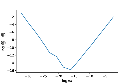
Figure 1: Natural logarithm of the modulus of the difference between the analytical and the finite-difference versions of $d\omega/da_{\text{analytical}}$ as a function of the natural logarithm of the step size. This is done for $a=0.68,s=-2,m=2$ and the overtone index $p=5$.

IV Improvements to the root-finding procedure

IV.1 General considerations

For a certain $a$, Eq. (4) when solved for the QNM frequency via numerical root-finding, gives a certain $\omega$. It is in this sense that we can write $\omega$ as a function of $a$; i.e. $\omega(a)$. This further allows us to write Eq. (II) as

$$\mathcal{C}(\omega,A,a)=\mathcal{C}(\omega(a),~{}A(c(a,\omega(a)))~{},a)=\mathcal{C}(a)=0,$$ (5)

Since Eq. (5) views $\mathcal{C}$ as a function of just one variable $a$, so that $d\mathcal{C}/da$ is a sensible quantity. Thus we have

$$\frac{d\mathcal{C}}{da}= \frac{\partial\mathcal{C}}{\partial\omega}\frac{d\omega}{da}+\frac{\partial\mathcal{C}}{\partial A}\frac{dA}{da}+\frac{\partial\mathcal{C}}{\partial a}=0$$ (6)

$$\frac{\partial\mathcal{C}}{\partial\omega}\frac{d\omega}{da}+\frac{\partial\mathcal{C}}{\partial A}\left[\frac{dA}{dc}\left(\frac{\partial c}{\partial a}+\frac{\partial c}{\partial\omega}\frac{d\omega}{da}\right)\right]+\frac{\partial\mathcal{C}}{\partial a}=0$$ (7)

$${\color[rgb]{0,0,0}\frac{\partial\mathcal{C}}{\partial\omega}}{\color[rgb]{0,0,0}\frac{d\omega}{da}}+{\color[rgb]{0,0,0}\frac{\partial\mathcal{C}}{\partial A}}\left[\frac{dA}{dc}\left(\omega+a{\color[rgb]{0,0,0}\frac{d\omega}{da}}\right)\right]+{\color[rgb]{0,0,0}\frac{\partial\mathcal{C}}{\partial a}}=0$$ (8)

$$\frac{d\omega}{da}= \frac{-\partial\mathcal{C}/\partial a-\omega~{}dA/dc~{}\partial\mathcal{C}/\partial a}{a~{}dA/dc~{}\partial\mathcal{C}/\partial A+\partial\mathcal{C}/\partial\omega}.$$ (9)

We also reproduce the expression of $dA/da$ in square braces in Eq. (8) for this, in addition to Eq. (9) will be useful for providing $\omega_{\text{guess}}$ and $A_{\text{guess}}$ at the next spin $a+\Delta a$ via linear extrapolation

$$\frac{dA}{da}=\frac{dA}{dc}\left(\omega+a\frac{d\omega}{da}\right).$$ (10)

IV.2 Improvements to the pre-existing algorithm of finding QNMs

The first improvement we propose is to provide the Newton-Raphson routine the $\omega$-derivative of the CF $\mathcal{C}$ in a closed-form. The $\omega$-derivative of $\mathcal{C}$ in Eq. (4) is computed as (with $a$ dependence suppressed because the context is that of a fixed BH spin $a$)

$$\frac{d\mathcal{C}(\omega,A(\omega))}{d\omega} =\frac{\partial\mathcal{C}(\omega,A)}{\partial\omega}+\frac{\partial\mathcal{C}(\omega,A)}{\partial A}\frac{dA}{d\omega},$$ (11)

$$=\frac{\partial\mathcal{C}(\omega,A)}{\partial\omega}+a\frac{\partial\mathcal{C}(\omega,A)}{\partial A}\frac{dA}{dc}.$$ (12)

The second proposal is in regard to the starting guesses (in the context of numerical root-finding) for QNM frequency $\omega$ and the eigenvalue $A$. We propose that at $a_{0}+\Delta a$, the guesses for $\omega$ and $A$ should be

$$\omega_{\text{guess}}=\omega_{0}+\frac{d\omega}{da}\bigg{|}_{a_{0},\omega_{0}}da,$$ (13)

$$A_{\text{guess}}=A_{0}+\frac{dA}{da}\bigg{|}_{a_{0},A_{0}}da,$$ (14)

where the total derivatives in the above two equations are to be computed using Eqs. (9) and (10). Now, to actually implement the above two improvements suggested in Eqs. (12), (13), and (14), we need to compute $dA/dc$ and the three partial derivatives of $\mathcal{C}$, i.e., $\partial\mathcal{C}/\partial a,\partial\mathcal{C}/\partial A$ and $\partial\mathcal{C}/\partial\omega$. This is the subject of the next section.

In light of Eqs. (4) and (12), we can discuss one more application of analytical derivatives . The QNM frequency is found by finding the root of $\mathcal{C}(\omega)=0$; here the $a$-dependence of $\mathcal{C}$ is suppressed. Now the software routines (like qnm [6]), have separate tolerances for checking the convergence of the CF $\mathcal{C}$, and numerical root-finding for $\mathcal{C}(\omega)=0$, and are usually set independently of each other. But now with the $d\mathcal{C}/d\omega$ information from Eq. (12), we can make the former depend on the latter. This can be done by setting

$$\Delta\mathcal{C}\sim\Delta\omega\frac{d\mathcal{C}}{d\omega},$$ (15)

where the symbol $\Delta$ before $\mathcal{C}$ and $\omega$ represents their respective tolerances. $\Delta\omega$ is usually decided on the basis of how accurately we want to determine the QNM frequencies, something that we need to consider while doing precise parameter estimation with GWs.

V Calculational details

V.1 Derivatives of a continued fraction

Before we deal with computing the derivatives of a CF, we will first discuss the challenges encountered when trying to compute them. We start with a typical CF

$$f(x)=b_{0}+\frac{a_{1}}{b_{1}+}\frac{a_{2}}{b_{2}+}\frac{a_{3}}{b_{3}+}\frac{a_{4}}{b_{4}+}\cdots,$$ (16)

where the quantities $a_{n}$’s and $b_{n}$’s are considered to be functions of a parameter $x$, and the aim is to differentiate $f(x)$ with respect to $x$. It is not hard to see that straightforward application of the basic rules of differentiation (product, quotient, and chain rules) to a finite-truncated version of the above CF will result in an explosion of the size of expression of the derivative, if a large number of terms are retained in $f(x)$. The requirement to store and process this large data on a computer algebra system like Mathematica can make the procedure inefficient and slow.

There is a more efficient way to compute the derivative of a CF. This rests on Lentz’s method of computing CFs (see Sec. 5.2 of Ref. [7] or Ref. [8]). The method dictates the following procedure to compute the CF

1. Set $f_{0}(x)=b_{0}(x)$, $C_{0}(x)=f_{0}(x)$ and $D_{0}(x)=0$.

2. For $j=1,2,\cdots$, we perform the following iterative procedure to obtain $f(x)$ to higher and higher accuracy (denoted by $f_{j}(x)$)
   

   $$D_{j}(x) =1/\left(b_{j}(x)+a_{j}(x)D_{j-1}(x)\right),$$ (17)

   $$C_{j}(x) =b_{j}(x)+a_{j}(x)/C_{j-1}(x),$$ (18)

   $$f_{j}(x) =f_{j-1}(x)C_{j}(x)D_{j}(x)$$ (19)

We terminate when $f_{j}$ appears to have converged sufficiently well. The task of processing through each value of $j$ can be called an iteration, which makes Lentz’s method an iterative procedure. This iterative procedure is the key to its efficiency. Note that while implementing the $n$th iteration, we need to store the information ($a_{j}$, $b_{j}$, $C_{j}$, $D_{j}$ and $f_{j}$) associated with $j=n$ and $j=n-1$. The information corresponding to smaller values of $j$ (which were used in the previous iterations) need not be stored. Apart from computing a CF, this efficient iterative procedure also lets us compute the derivative of the CF in a similar “Lentz-like” way, as we now explain.

To compute the derivative of a CF, proceed along the same enumerated steps of Lentz’s method as above, but after the second step, add a third step to the iteration given by

1. For $j=1,2,\cdots$, we perform
   

   $$D^{\prime}_{j}(x) =-\frac{D_{j-1}(x)a^{\prime}_{j}(x)+b^{\prime}_{j}(x)+a_{j}(x)D^{\prime}_{j-1}(x)}{(b_{j}(x)+a_{j}(x)D_{j-1}(x))^{2}},$$ (20)

   $$C^{\prime}_{j}(x) =\frac{1}{(C_{j-1}(x))^{2}}\left[C_{j-1}(x)a^{\prime}_{j}(x)\right.$$

   $$\left.+(C_{j-1}(x))^{2}b_{j}^{\prime}(x)-a_{j}(x)C^{\prime}_{j-1}(x)\right],$$ (21)

   $$f^{\prime}_{j}(x) =C_{j}(x)D_{j}^{\prime}(x)f_{j-1}(x)$$

   $$+D_{j}(x)(f_{j-1}(x)C_{j}^{\prime}(x)+C_{j}(x)f_{j-1}^{\prime}(x)).$$ (22)

The above three equations are results of the application of basic rules of differentiation on Eqs. (17)-(19). Here we have assumed that the evaluation of $a_{j}^{\prime}(x)$ and $b_{j}^{\prime}(x)$ is tractable. This basically turns the evaluation of $f_{j}^{\prime}(x)$ into an iterative Lentz-like procedure which we terminate when a reasonable degree of convergence has been achieved. This is how we compute $\partial\mathcal{C}/\partial a,\partial\mathcal{C}/\partial A$ and $\partial\mathcal{C}/\partial\omega$.

V.2 Eigenvalue of a perturbed complex-symmetric matrix

From Eq. (2) (an eigenvalue equation), we can see that ${}_{s}A_{\ell m}\equiv A$ is a $c$-dependent eigenvalue, which further means that the task of computing $dA/dc$ is that of computing the rate of change of the eigenvalue with respect to a variable that parameterizes the eigenvalue problem. This problem appears to be similar to that of quantum mechanical perturbation theory, or the Rayleigh-Schrodinger perturbation theory (RSPT); see Chapter 6 of Ref. [9]. But there is one important difference. In the RSPT, the operator or the matrix (perturbed and unperturbed) whose eigenvalues are the subject of discussion is a Hermitian one, whereas here the matrix $\mathbb{M}(c)$ in Eq. (2) is not Hermitian but rather complex-symmetric. How then can we modify the RSPT to adapt to this situation where the matrices are complex-symmetric, rather than Hermitian? We answer this question below.

Because our solution to the complex-symmetric matrix eigenvalue perturbation problem is a modification of the popular solution to the Hermitian matrix eigenvalue perturbation problem (typically encountered in quantum mechanics), we have chosen to use Dirac’s bra-ket notation, but with a slight modification. $\ket{a}$ as usual, represents a column vector but $\bra{a}$ will stand for the transpose of $\ket{a}$, rather than its conjugate transpose. Hence,

$$\langle a\mid b\rangle\equiv a^{T}b,~{}~{}~{}~{}~{}~{}\langle a|\mathbb{M}|b\rangle\equiv a^{T}\mathbb{M}b.$$ (23)

Now, the unperturbed and the perturbed eigenvalue equations are

$$H_{0}\left|n_{0}\right\rangle =E^{0}\left|n_{0}\right\rangle,$$ (24)

$$\left(H_{0}+V\right)|n\rangle =(E^{0}+\Delta)|n\rangle,$$ (25)

respectively. Here $H_{0}$ and $E^{0}$ are the unperturbed complex-symmetric matrix, and the associated unperturbed eigenvalue, respectively. We have used $\ket{n_{0}}$ to denote the unperturbed eigenvector. $V$, $\Delta$ and $\ket{n}$ are the complex-symmetric perturbation matrix, the perturbation in the eigenvalue, and the perturbed eigenvector, respectively. The above equation gives us

$$\left\langle n_{0}\left|\left(E^{0}-H_{0}\right)\right|n\right\rangle=\left\langle n_{0}|(V-\Delta)|n\right\rangle.$$ (26)

Since $H_{0}$ is a complex-symmetric matrix, it can be easily shown for any general vectors $\ket{a}$ and $\ket{b}$ with complex entries, that $\left\langle a\left|H_{0}\right|b\right\rangle=\left\langle b\left|H_{0}\right|a\right\rangle$. This, along with $\braket{a}{b}=\braket{b}{a}$ makes it possible to write Eq. (26) as

$$\left\langle n_{0}|(V-\Delta)|n\right\rangle= \left\langle n_{0}\left|E^{0}\right|n\right\rangle-\left\langle n_{0}\left|H_{0}\right|n\right\rangle$$

$$= \left\langle n_{0}\left|E^{0}\right|n\right\rangle-\left\langle n\left|H_{0}\right|n_{0}\right\rangle$$

$$= E^{0}\left(\left\langle n_{0}\mid n\right\rangle-\left\langle n\mid n_{0}\right\rangle\right)=0.$$ (27)

This finally yields

$$\left\langle n_{0}|(V-\Delta)|n\right\rangle=0$$ (28)

$$\Delta=\frac{\left\langle n_{0}|V|n\right\rangle}{\left\langle n_{0}\mid n\right\rangle}=\frac{\left\langle n_{0}|V|n_{0}\right\rangle}{\left\langle n_{0}\mid n_{0}\right\rangle}.$$

To arrive at the last result, we replaced $\ket{n}$ with $\ket{n_{0}}$. This is justified because it makes a difference at a higher order in perturbation scheme than what we are concerned here.

VI Software package

We have implemented the improvements suggested in Sec. IV.2, based on the first derivative information in a Git-forked version of the original Python package qnm that was introduced with Ref. [6]. This forked repository can be found at Ref. [10]. At a certain fixed BH spin $a$, preliminary investigation suggests that with these improvements, the root-finding procedure is faster by a factor of 1.5 when compared with the original qnm package of Ref. [6]. Since this is done only at a fixed $a$, the analytical derivatives $d\omega/da$ and $dA/da$ do not matter. This speed boost could be due to supplying the analytical derivative $d\mathcal{C}/d\omega$ to the Newton-Raphson routine, as discussed in Sec. IV.2. The reason we do not make comparisons while changing the BH spin $a$ is that the original qnm package uses numerical second derivative (in the form of quadratic fits and extrapolation) to predict $\omega_{\text{guess}}$ and $A_{\text{guess}}$ at various $a$’s, whereas the forked version of the package makes this prediction on the basis of only the first (analytical) derivatives. We plan to make these comparisons once the analytical second derivative information is also included in the package in the future.

VII Summary

In this paper, we have laid the theoretical groundwork to make the spectral variant of Leaver’s method of finding the QNM frequencies more robust. This is done by introducing ways to compute the necessary derivatives analytically rather than numerically. We have confined ourselves to first derivatives only, leaving the work on second derivatives for future work. Our work should be particularly useful when the QNM frequency trajectory (as the BH spin $a$ is varied) in the complex plane has large curvature. We have incorporated the first derivative information in the Python package qnm.

We saw in Sec. III that inclusion of the second derivative information can let us take large step size in the BH spin $a$. This, combined with the fact that it is the second derivative (rather than the first derivative) that lets us decide the right step size to take when using the adaptive step size approach, makes the prospect of extending our present work to include second derivatives, the most natural future course of action. Thereafter, one can include the analytical second derivative information too in the qnm Python package that was introduced with Ref. [6]. Comparisons can then be made to assess the improvements brought about by computing derivatives analytically rather than numerically. These can be in regard to the speed of finding the QNM frequencies, the size of the step in the BH spin $a$ that we can safely take, the robustness of the routine (can it find the QNM frequencies that the present routines can’t), among others. There is not much point in pushing our derivative calculations to very high orders. This is because after a certain point, due to the high order of the analytical derivative being computed, the computational overhead will start to outweigh the gains it may bring. Finally, there is also hope to adapt our work to find QNM frequencies in some modified theories of gravity, provided in those theories, the QNM frequencies are found using a method that is a variant of Leaver’s method.

References

- Berti et al. [2009] E. Berti, V. Cardoso, and A. O. Starinets, Quasinormal modes of black holes and black branes, Class. Quant. Grav. 26, 163001 (2009), arXiv:0905.2975 [gr-qc] .
- Nollert [1999] H.-P. Nollert, Quasinormal modes: the characteristic `sound' of black holes and neutron stars, Classical and Quantum Gravity 16, R159 (1999).
- Leaver [1985] E. W. Leaver, An Analytic representation for the quasi normal modes of Kerr black holes, Proc. Roy. Soc. Lond. A 402, 285 (1985).
- Cook and Zalutskiy [2014] G. B. Cook and M. Zalutskiy, Gravitational perturbations of the Kerr geometry: High-accuracy study, Phys. Rev. D 90, 124021 (2014), arXiv:1410.7698 [gr-qc] .
- Hughes [2000] S. A. Hughes, The Evolution of circular, nonequatorial orbits of Kerr black holes due to gravitational wave emission, Phys. Rev. D 61, 084004 (2000), [Erratum: Phys.Rev.D 63, 049902 (2001), Erratum: Phys.Rev.D 65, 069902 (2002), Erratum: Phys.Rev.D 67, 089901 (2003), Erratum: Phys.Rev.D 78, 109902 (2008), Erratum: Phys.Rev.D 90, 109904 (2014)], arXiv:gr-qc/9910091 .
- Stein [2019] L. C. Stein, qnm: A Python package for calculating Kerr quasinormal modes, separation constants, and spherical-spheroidal mixing coefficients, J. Open Source Softw. 4, 1683 (2019), arXiv:1908.10377 [gr-qc] .
- Press et al. [2007] W. Press, S. Teukolsky, W. Vetterling, and B. Flannery, Numerical Recipes 3rd Edition: The Art of Scientific Computing (Cambridge University Press, 2007).
- Press and Teukolsky [1988] W. H. Press and S. A. Teukolsky, Evaluating continued fractions and computing exponential integrals, Computers in Physics 2, 88 (1988), https://aip.scitation.org/doi/pdf/10.1063/1.4822777 .
- Griffiths and Schroeter [2018] D. Griffiths and D. Schroeter, Introduction to Quantum Mechanics (Cambridge University Press, 2018).
- [10] https://github.com/sashwattanay/qnm.