Superconductivity in a system of interacting spinful semions

Abstract

Non-interacting particles obeying certain fractional statistics have been predicted to exhibit superconductivity. We discuss the issue in an attractively interacting system of spinful semions on a lattice by numerically investigating the presence of off-diagonal long-range order at zero temperature. For this purpose, we construct a Hubbard model wherein two semions with opposite spin can virtually coincide while maintaining consistency with the fractional braiding statistics. Clear off-diagonal long range order is seen in the strong coupling limit, consistent with the expectation that a pair of semions obeys Bose statistics. We find that the semion system behaves similarly to a system of fermions with the same attractive Hubbard $U$ interaction for a wide range of $U$, suggesting that semions also undergo a BCS to BEC crossover as a function of $U$.

I Introduction

The topology of configuration space determines the possible quantum statistics of a system of identical particles [1]. In two dimensions, the fundamental group of the many-particle configuration space is the braid group, which allows exotic particles, namely anyons [2], that obey statistics beyond bosons and fermions. The emergence of anyons as elementary excitations is a defining feature of the so-called topological order [3], which has demonstrated how topology enriches phases of matter beyond Landau’s symmetry-breaking paradigm. A typical example of topologically ordered phases is the fractional quantum Hall effect [4]. Special properties such as (non-Abelian) anyon excitations [5, 6, 7], fractional charges [8], and the topological degeneracy [9, 10] are closely related to each other [3, 11, 12, 13, 14]. Quantum spin liquids [15, 16, 17] and topological superconductors [18, 19, 20, 21, 22, 23] are also promising platforms that harbor anyons, which are not only fundamentally interesting in their own right but also have attracted considerable attention for their potential for quantum computation [24, 25].

Understanding the behavior of quantum anyon gases is a fundamentally interesting problem. An exchange of $n$ Abelian anyons with statistical angle $\theta$ gives the phase factor $e^{in^{2}\theta}$. This implies that $p$-tuples with $\theta=\pi(1-1/p)$ behave as bosons and thus may condense to form a superfluid [26, 27, 28, 29]. Historically, anyon superconductors, especially with $\theta=\pi/2$ (semions), have been extensively studied for their possible relevance to the high-$T_{c}$ superconductivity of the copper oxides [30, 31, 32]. In theoretical studies, the identification of off-diagonal long-range order (ODLRO) is convincing evidence of superconductivity. The system of semions may be mapped to the $\nu=2$ integer quantum Hall system by trading the statistical fluxes for uniform magnetic ones. This mean field theory produces algebraic ODLRO in the $2$-body reduced density matrix [33, 34]. There also exists an exactly solvable model of spinful semions beyond the mean field description, which exhibits (not just algebraic) ODLRO [35, 36]. In this paper, we revisit this problem by developing a method to construct the Hubbard model of anyons.

The main goal of this work is to numerically confirm ODLRO for attractively interacting spinful semions in a lattice system. When fermions attractively interact, BCS pairs develop which are appropriately described by Bose-Einstein condensation (BEC) in the strong coupling limit [37, 38]. Correspondingly, their ground states are expected to exhibit ODLRO in the two-body reduced density matrix. By comparing the behavior of ODLRO for semions and fermions, we investigate whether the BCS-BEC crossover occurs in semionic systems. In the limit of large interaction strength, the system of semions is expected to exhibit the same behavior as a system of fermions with large Hubbard interaction strength, since pairs of semions and pairs of fermions both obey mutual Bose statistics. In the weakly interacting regime, systems of fermions behave differently from the BEC state and there is no clear connection between semionic and fermionic systems.

We start with a construction of the Hubbard model of anyons with tunable on-site interactions. This is not a straightforward generalization of the tight-binding model for spinless anyons [39, 40, 41, 42, 43, 44, 45] into a spinful problem. Since anyons carry fractional statistics, two particles may not coincide even if their spins are different, which makes it nontrivial to set up a model with a finite on-site Hubbard $U$ interaction. We overcome this difficulty by virtually splitting sites for each spin, thereby fixing the way that particles with different spin pass one another. Within this framework, we present a careful construction of the Hubbard model of anyons and define the reduced density matrix for two semions. We numerically demonstrate clear ODLRO for semions in the strong coupling limit. We find that the reduced density matrices for semions and for fermions behave similarly in a wide range of $U$. This suggests that a BCS-BEC crossover occurs in semionic systems.

II Hubbard model for anyons

II.1 Spinless anyons on a torus: the string gauge

We begin by reviewing the hopping Hamiltonian of spinless anyons on a torus [39, 40, 41, 43]. The statistical angle is set as $\theta/\pi=n/m$ with $n,m$ coprime. The Hilbert space for the system with $N$ particles is spanned by the basis $\ket{\{\bm{r}_{k}\};w}$, where $\{\bm{r}_{k}\}$ labels $N$ occupied sites and $w$ labels an additional internal degree of freedom required by topology of the torus. The label $w$ takes integer values from 1 to $m$. By modeling anyons as bosons with statistical fluxes, the Hamiltonian with nearest-neighbor hopping is given by [39, 40, 41, 43]

$$H=-t\sum_{\langle ij\rangle}c_{i}^{\dagger}e^{i\theta_{ij}}W_{ij}c_{j},$$ (1)

where $c^{\dagger}_{i}$ is the creation operator for a hard-core boson on site $i$. The hard-core condition is necessary to ensure consistency with the braid group: if particles can coincide, the system allows only Bose statistics [1]. The phase factor $e^{i\theta_{ij}}$ describes the statistical phase for a particle exchange. $W_{ij}$ is an $m$-dimensional matrix associated with the degree of freedom $w$, which describes phase factors arising from global moves of anyons on a torus. For $\theta/\pi=1$, $e^{i\theta_{ij}}$ produces the sign $\pm 1$, resulting in $H$ reducing to the standard Hamiltonian of noninteracting fermions.

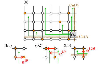
Figure 1: (a) Sketch of a $6\times 4$ lattice with $N=7$ particles with the string gauge (green arrows). The brown lines represent the cuts A and B. (b1) Rule $\theta_{ij}$:(i). (b2) Rule $\theta_{ij}$:(ii). (b3) Rule $\theta_{ij}$:(iii).

The assignment of $\theta_{ij}$ is obtained by strings placed on the lattice as shown in Fig. 1(a). These strings emanate from the origin represented by $O_{\theta}$, and terminate in the lower-right plaquette adjacent to each particle. They run first from right to left and then turn in the vertical direction at a proper plaquette. We also set cuts labeled A and B as shown in Fig. 1(a). Using these strings, we first assign $\theta_{ij}$ and $W_{ij}$ for a hopping that does not cross the cuts:

1. If an anyon hops from left to right across a string, it acquires the phase factor $e^{i\theta}$ [Fig. 1(b1)].

2. If a string sweeps another anyon in the process of hopping, the phase factor is gained as if the anyon crosses the string [Fig. 1(b2)].

1. The index $w$ does not change. This corresponds to $W_{ij}=\bm{1}_{m}$ ($m$-dimensional identity matrix).

These rules ensure that the basis states $\ket{\{\bm{r}_{k}\};w}$ acquire the statistical phase $e^{i\theta}$ whenever one takes two anyons and swaps their positions without crossing the cuts. For a hopping across the cuts, we need to set other rules as follows: (Here we assume that an anyon hops across the cut A upward or the cut B from left to right.)

1. (Cut A) The phase factor $e^{i2\theta}$ (not $e^{i\theta}$) is gained if an anyon crosses a string [Fig. 1(b3)].

2. (Cut A) $e^{iX\theta}$ is given, where $X$ is the number of other anyons that have the same $x$ coordinate as the hopping anyon.

3. (Cut B) One determines the phase factor obeying the rules (i) and (ii) and then rearranges the horizontal part of the string.

4. (Cut B) The phase factor $e^{i(N-1)\theta}$ occurs.

1. (Cut A) The phase factor $e^{iw\theta}$ is given ($w$ is the additional internal degree of freedom mentioned above). This corresponds to

   $$W_{ij}=W_{y}\equiv\text{diag}[e^{i2\theta},e^{i4\theta},\ldots,e^{i2m\theta}].$$ (2)

2. (Cut B) The index $w$ is changed to $w-1$. This corresponds to

   $$W_{ij}=W_{x} \equiv\left[\begin{array}[]{cccc}0&1&\ldots&0\\ \vdots&\vdots&\ddots&\vdots\\ 0&0&\ldots&1\\ 1&0&\ldots&0\end{array}\right].$$ (7)

The above rules for $\theta_{ij}$ imply that $\theta_{ij}$ can be written in the following form:

$$\theta_{ij}=\sum_{k\neq i,j}A_{ij}^{k}n_{k},$$ (8)

where $A_{ij}^{k}$ is a real number determined from the rules given above and $n_{k}=c_{k}^{\dagger}c_{k}$. The rules $W_{ij}$:(ii) and (iii) are required for some algebraic constraints of the braid group on a torus: operators $\tau_{i}$ and $\rho_{i}$ that move the $i$th particle along a noncontractible loop in the $x$ and $y$ direction, respectively, satisfy $\rho_{i}^{-1}\tau_{j}\rho_{i}\tau_{j}^{-1}=B_{ij}$, where $B_{ij}$ is an operator that moves the $i$th particle around the $j$th particle along a closed loop. This is consistent with the fact that we have $B_{ij}=e^{i2\theta}$ and

$$W_{y}^{-1}W_{x}W_{y}W_{x}^{-1}=e^{i2\theta}.$$ (9)

The rules $\theta_{ij}$:(iii) and (vi) also play a role to remove the artificial twisted boundary condition caused by the anyon fluxes. The twisted boundary conditions are introduced by modifying the matrices as $W_{x}\rightarrow e^{i\eta_{x}}W_{x}$ and $W_{y}\rightarrow e^{i\eta_{y}}W_{y}$, where $\eta_{x}$ and $\eta_{y}$ are the twisted boundary condition angles.

II.2 Generalization to spinful system

Let us generalize the above formulation into a system of spinful anyons on a lattice. The statistical phase for an exchange of anyons with the same spin is set as $e^{i\theta}$. Note that the statistical phase is not well defined for an exchange of opposite spins since this operation does not form a closed loop in configuration space. Instead, two consecutive operations, which is equivalent to a move of a spin $\uparrow$ around a spin $\downarrow$ or vice versa (this is referred to as “local move” below), forms a closed loop in the configuration space. We assign to this the phase factor $e^{i2\theta}$, i.e., a local move of a particle around another particle produces the phase factor $e^{i2\theta}$ whether or not they have the same spin.

Incorporating the on-site interaction between anyons with opposite spins, we write the Hamiltonian in the form of the Hubbard model:

$$H=-t\sum_{\langle ij\rangle}\sum_{\alpha=\uparrow,\downarrow}c_{i\alpha}^{\dagger}e^{i\theta_{ij\alpha}}W_{ij\alpha}c_{j\alpha}+U\sum_{i}n_{i\uparrow}n_{i\downarrow},$$ (10)

where $n_{i\alpha}=c_{i\alpha}^{\dagger}c_{i\alpha}$ and $c_{i\alpha}^{\dagger}$ is the creation operator for a spinful hard-core boson satisfying $c_{i\uparrow}^{\dagger 2}=c_{i\downarrow}^{\dagger 2}=0$. As in the spinless case, $\theta_{ij\alpha}$ depends on the number operators of all sites and, therefore, $e^{i\theta_{ij\alpha}}$ generates complicated non-local many-body interactions. This nature makes it quite difficult to apply effective formalisms such as the Bogoliubov-de Gennes treatment. The construction of $\theta_{ij\alpha}$ and $W_{ij\alpha}$ is described below.

II.2.1 $U=+\infty$

The system with the hard-core constraint $c_{i\uparrow}^{\dagger}c_{i\downarrow}^{\dagger}=0$ (equivalently $U=+\infty$) is given by a simple generalization of the formulation for spinless anyons [45]. The Hilbert space is spanned by the basis $\ket{\{\bm{r}_{j}\},\{\bm{r}_{k}\};w}$ with $j=1,\ldots,N_{\uparrow}$ and $k=1,\ldots,N_{\downarrow}$, where $N_{\alpha}$ is the particle number with spin $\alpha$, $\{\bm{r}_{j}\}$ and $\{\bm{r}_{k}\}$ label sites occupied by spin $\uparrow$ and $\downarrow$, respectively. Here the sets of positions $\{\bm{r}_{j}\}$ and $\{\bm{r}_{k}\}$ are disjoint. One can construct this from the spinless basis $\ket{\{\bm{r}_{l}\};w}$ with $l=1,\ldots,N$ by partitioning positions into two groups of $N_{\uparrow}$ and $N_{\downarrow}$ each, where $N=N_{\uparrow}+N_{\downarrow}$. Due to the multiple ways of making this partition, the dimension of the Hilbert space is $N!/(N_{\uparrow}!N_{\downarrow}!)$ times larger than that for the corresponding spinless system. Using this basis, we consider the Hamiltonian in Eq. (10) with

$$\theta_{ij\uparrow}=\theta_{ij\downarrow}=\theta_{ij},$$ (11)

$$W_{ij\uparrow}=W_{ij\downarrow}=W_{ij}$$ (12)

where $\theta_{ij}$ and $W_{ij}$ have been defined in the spinless problem (we redefine $\theta_{ij}$ in Eq. (8) with $n_{k}=n_{k\uparrow}+n_{k\downarrow}$). As ensured by the above rules (i)-(iii), the phase factors $e^{i\theta}$ and $e^{i2\theta}$ are given for an exchange of particles with the same spin and for a local move of a particle around another, respectively. This system has SU(2) spin-rotational symmetry since $\theta_{ij\alpha}$ is invariant under the transformation $\bm{c}_{i}^{\dagger}\rightarrow\bm{c}_{i}^{\dagger}u$ with $u\in\text{SU(2)}$, where $\bm{c}_{i}^{\dagger}\equiv(c_{i\uparrow}^{\dagger},c_{i\downarrow}^{\dagger})$.

II.2.2 Finite $U$

The system with finite $U$ allows for double occupancy of sites as shown in Fig. 2(a). We note here that whether or not such a system can be well-defined is itself a nontrivial problem. As mentioned above, moving a spin $\uparrow$ around a spin $\downarrow$ or vice versa along a closed loop gives the phase factor $e^{i2\theta}$, implying that the positions of particles are singular points unless $e^{i2\theta}=1$. This feature appears to prohibit an unambiguous identification of the phase factor for a local move shown in Fig. 2(b), where two anyons with opposite spins coincide in the process.

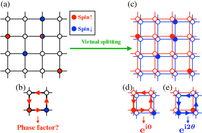
Figure 2: (a) Sketch of a $4\times 4$ lattice with the particle numbers $N_{\uparrow}=N_{\downarrow}=3$. (b) Local move of an anyon with spin $\uparrow$. The red arrows represent the direction of the hopping. The phase factor is generally not well-defined due to the coincidence of spin-up and spin-down particles along the path of the spin-up particle. (c) Virtual splitting. (d)-(e) Local moves of anyons with (d) spin $\uparrow$ and (e) spin $\downarrow$. The bold lines and its arrows represent the paths and the direction of the hoppings. Because of the virtual splitting, each phase factor is uniquely determined.

This ambiguity can be resolved by virtually splitting the sites and thereby fixing the way the particles pass around each other. As shown in Fig. 2(c), let us shift the sites for spin $\downarrow$ particles infinitesimally in the south east direction. This configuration enables us to see whether anyons are enclosed or not for a given local move. Accordingly, the phase factor is uniquely determined since the path of the spin $\uparrow$ particle does not enclose the spin $\downarrow$ particle in Fig. 2(d), whereas the path of the spin $\downarrow$ particle encloses the spin $\uparrow$ particle, as seen in Fig. 2(e).

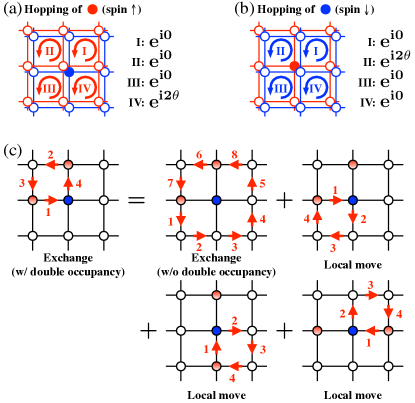
Figure 3: (a)(b) Four plaquettes adjacent to an anyon with (a) spin $\downarrow$ and (b) spin $\uparrow$. Each plaquette is labeled by I$,\ldots,$IV. The hoppings of (a) spin $\uparrow$ and (b) spin $\downarrow$ along each plaquette give the phase factors as listed on the right in each figure. (c) An exchange operation of two anyons with spin $\uparrow$ is decomposed into four parts: an exchange with no double occupancy on any site and local moves involving the double occupancy. The numbers written next to the arrows indicate the order of operation.

We have not included terms with $n_{i\alpha}$ or $n_{j\alpha}$ in $\theta_{ij\beta}$ in Eq. (11) so far because of the hard-core nature of the anyons. To incorporate the virtual splitting, we now add terms such as $\theta_{ij\alpha}=\theta_{ij}+D_{ij\alpha}$, where

$$D_{ij\uparrow}=A_{ij}^{i\downarrow}n_{i\downarrow}+A_{ij}^{j\downarrow}n_{j\downarrow},$$ (13)

$$D_{ij\downarrow}=A_{ij}^{i\uparrow}n_{i\uparrow}+A_{ij}^{j\uparrow}n_{j\uparrow}.$$ (14)

The coefficients $A_{ij}^{i\alpha}$ are assigned as follows. We put an anyon with spin $\downarrow$ on a site, see Fig. 3(a). We then design rules of $A_{ij}^{i\downarrow}$ so that the phase accumulated by moving spin $\uparrow$ along each adjacent plaquette matches with the virtual splitting. Each phase is listed on the right in the figure. We also determine $A_{ij}^{i\uparrow}$ in the same way, see Fig. 3(b). These conditions regarding only four adjacent plaquettes are sufficient to design $A_{ij}^{i\alpha}$ as can be seen from the following example. An exchange operation shown in Fig. 3(c), where double occupancy occurs, can be decomposed into several operations that are well-defined in the above framework: an exchange operation involving no double occupancy and local moves along a plaquette. This implies that the exchange operation before the decomposition should give the proper phase that reflects the virtual splitting. Other operations in which double occupancy occurs also give proper phase factors since these can be decomposed in the same way as above.

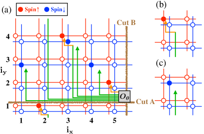
Figure 4: (a) Sketch of a $5\times 4$ lattice with $N_{\uparrow}=N_{\downarrow}=3$ with the string gauge (green or orange arrows). The brown lines represent the cut A and the cut B. (b)(c) String for (b) spin $\uparrow$ and (c) spin $\downarrow$.

We now give an explicit construction of $A_{ij}^{i\alpha}$ by modifying the rules for the strings. Figure 4(a) pictorially shows the strings attached to each particle with the virtual splitting. The assignment of strings is almost the same as the spinless case, since we do not change the form of $\theta_{ij\alpha}$ in Eq. (11) except for the addition of new terms $D_{ij\alpha}$. The difference is in the vicinity of particles as shown in Figs. 4(b) and (c), where we introduce a new orange string around spin $\uparrow$. Using these, we employ the previous rules $\theta_{ij}$:(i)-(vi), but change only the rule $\theta_{ij}$:(iii) as

1. (Cut A) The phase factor $e^{i2\theta}(e^{i\theta})$ is given if an anyon crosses a green (orange) string.

We still use Eq. (12) for $W_{ij\alpha}$ without any modification.

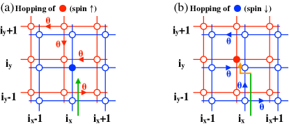
Figure 5: Hopping phases of an anyon with (a) spin $\uparrow$ and (b) spin $\downarrow$. The label of the site $(i_{x},i_{y})$ satisfies $3\leq i_{y}\leq N_{y}$ (no restriction on $i_{x}$). The sum of phases along each link is consistent with the virtual splitting.

The above rules clearly produce the phase factor shown in Figs. 3(a) and (b). Figure 5 shows the hopping phases assigned to each link. Here we assume $3\leq i_{y}\leq N_{y}$ (no restriction on $i_{x}$), where $i_{x(y)}$ is the label of sites, see Fig. 4(a). Clearly, the sum of the hopping phases along each plaquette matches with the virtual splitting. Other situations (namely, $\vec{i}$ with any $i_{x}$ and $1\leq i_{y}\leq 2$) are discussed in Appendix A.

Because of the virtual splitting, $\theta_{ij\alpha}$ no longer takes the form $\sum_{k\neq i,j}A_{ij}^{k}(n_{k\uparrow}+n_{k\downarrow})$. This breaks SU(2) spin-rotational symmetry unless $\theta/\pi$ is an integer. If particles are fermions or bosons, our model reduces to the standard Hubbard model or the spinful Bose-Hubbard model with hard-core interactions between bosons with the same spin. Although the absence of SU(2) symmetry for anyons is just an artificial effect due to the virtual splitting, we stress that the fractional statistics is well-defined without ambiguity in our model. This method enables us to effectively investigate an interplay between the short-range interaction and the fractional statistics for systems that we can deal with using the exact diagonalization method.

II.2.3 $U\ll-1$

Let us discuss the effective Hamiltonian in the strong interaction limit $U\ll-1$. We denote the first and second terms in Eq. (10) by $H_{\text{kin}}$ and $H_{\text{int}}$, respectively, and we consider $H_{\text{kin}}$ as a perturbation to $H_{\text{int}}$. In the unperturbed problem, the ground state forms pairs of anyons at each site. This macroscopic degeneracy is lifted by the second-order perturbation: $H^{\prime}=PH_{\text{kin}}Q\frac{1}{E_{0}-H_{\text{int}}}QH_{\text{kin}}P$, where $P$ is the projection operator to the degenerate ground state, $H_{\text{int}}P=E_{0}P$ and $Q=1-P$.

For $\theta/\pi=1$ (fermions), we have $H^{\prime}=(2t^{2}/U)\sum_{\langle ij\rangle}b^{\dagger}_{i}b_{j}$ as shown in Appendix B, where $b_{i}^{\dagger}$ is the creation operator for a hard-core boson. We ignore a term which is constant when the particle number is fixed. The boundary conditions of $H^{\prime}$ and $H$ satisfy $(\eta^{\prime}_{x},\eta_{y}^{\prime})=(2\eta_{x},2\eta_{y})$. The expression of $H^{\prime}$ for general $\theta$ is complicated but we can deduce it by considering the statistics of a pair. For instance, pairs of semions with $\theta/\pi=1/2$ behave like bosons, implying that the effective Hamiltonian is given by

$$H^{\prime}=(2t^{2}/U)\sum_{\langle ij\rangle}b^{\dagger}_{i}b_{j}\bm{1}_{2},$$ (15)

where the identity matrix $\bm{1}_{2}$ comes from $W_{x}^{2}=W_{y}^{2}=\bm{1}_{2}$ [see Eqs. (2) and (7) with $m=2$], which leads to a 2-fold degeneracy. The boundary conditions satisfy $(\eta^{\prime}_{x},\eta_{y}^{\prime})=(2\eta_{x}+\pi,2\eta_{y}+\pi)$. The shift of $\pi$ follows from the fact that the rules we constructed using strings produce the phase factor $-1$ apart from the twisted boundary conditions when one moves a pair of semions along a noncontractible loop in the $x$ or $y$ direction [46].

II.3 Two-body reduced density matrix

To investigate the presence of ODLRO for these systems, we now define the two-body reduced density matrix as  [34, 36]

$$\rho(i,j)=\bra{\Psi}T_{ij}\ket{\Psi},$$ (16)

$$T_{ij}=\prod_{\langle kl\rangle\in L_{ij}}\left[c_{k\uparrow}^{\dagger}e^{i\theta_{kl\uparrow}}W_{kl\uparrow}c_{l\uparrow}c_{k\downarrow}^{\dagger}e^{i\theta_{kl\downarrow}}W_{kl\downarrow}c_{l\downarrow}\right]$$ (17)

where $\ket{\Psi}$ is the ground state of $H$ and $\prod_{\langle kl\rangle\in L_{ij}}$ indicates the products over all the links of a path, $L_{ij}$, starting from $j$ to $i$. For a given basis state $\ket{\{\bm{r}_{j}\},\{\bm{r}_{k}\};w}$, we choose the path $L_{ij}$ so that (i) there is no particle along it except for the site $j$ and (ii) all paths for any basis states are continuously connected with each other (i.e., two paths for two basis states always form a contractible loop on a torus).

The value of $\rho(i,j)$ is independent of the choice of the path $L_{ij}$ if $\theta/\pi=\mathbb{Z}/2$. To see this, consider two paths $L_{ij}$ and $L_{ij}^{\prime}$. Since the two paths form a closed loop, denoted by $(L_{ij}^{\prime})^{-1}L_{ij}$, the corresponding operators $T_{ij}$ and $T_{ij}^{\prime}$ satisfy

$$T_{ij}^{\prime-1}T_{ij}\ket{\{\bm{r}_{k}\},\{\bm{r}_{l}\};w}=e^{i4n\theta}\ket{\{\bm{r}_{k}\},\{\bm{r}_{l}\};w},$$ (18)

where $n$ is the number of anyons enclosed by the closed loop, and the sites $i$ and $j$ are assumed to be occupied in the basis state. This implies $T_{ij}\ket{\{\bm{r}_{k}\},\{\bm{r}_{l}\};w}=T^{\prime}_{ij}\ket{\{\bm{r}_{k}\},\{\bm{r}_{l}\};w}$ for $\theta/\pi=\mathbb{Z}/2$, i.e., $\rho(i,j)$ is path-independent. [For $\theta/\pi=1$, $\rho(i,j)$ is equivalent to the standard reduced matrix for fermions.]

Anyonic systems should be invariant under a many-particle translation since the statistical gauge field should depend only on relative coordinates of each pair of particles [2]. This implies that our Hamiltonian satisfies $GTH(\eta_{x},\eta_{y})T^{\dagger}G^{\dagger}=H(\eta_{x},\eta_{y})$, where $T$ is a translational operator and $G$ is a gauge transformation that rearranges the configuration of strings. Since $|\rho(i,j)|$ is a gauge invariant, the relation $|\rho(i,j)|=|\rho(i+\delta,j+\delta)|$ should hold for any translation $\delta=(\delta_{x},\delta_{y})$. We numerically confirm this as mentioned below.

III Results

We consider a system with 6 fermions or 6 semions on a $6\times 6$ lattice by using the above setup. The inter-particle distance is $r_{0}=a\sqrt{(6\times 6)/6}\approx 2.45a$, where $a$ is the lattice constant. We set $t=1$ and $U\leq 0$. The system of attractively interacting fermions produces superconducting states, which is demonstrated by the appearance of ODLRO (discussed below). We also compute the superconducting order parameter in Appendix C. By comparing the reduced density matrix $\rho(i,j)$ for semions and fermions, we identify the emergence of semion superconductivity.

III.1 Spectral flow

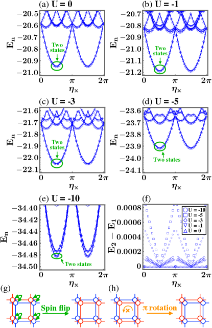
Figure 6: (a)-(e) Spectral flows for semions at (a) $U=0$, (b) $U=-1$, (c) $U=-3$, (d) $U=-5$ and (e) $U=-10$. The system size is $6\times 6$ and the particle number is $N=6$. The twist angle in the $y$-direction is set as $\eta_{y}=0$. The circles indicate $S_{z}=0$. The squares that appear only in (a)-(c) indicate $S_{z}=1$. States with larger $S_{z}$ not shown here have higher energies outside the figure. The lowest 5 energies at each $\eta_{x}$ and $S_{z}$ are plotted. (f) Energy gap between the two states indicated by the green circles in (a)-(e). (g)(h) Pictorial explanation of the unitary operator $R$: (g) the spin-flip and (h) the $\pi$ rotation.

We first investigate the energy spectrum for semions. In Figs. 6(a)-(e), we plot the energy as a function of the twisted boundary condition angle in the $x$-direction $\eta_{x}$. We here set $\eta_{y}=0$. The ground state always gives $S_{z}=0$ at any $\eta_{x}$. The eigenenergies have a periodicity $E_{n}(\eta_{x},\eta_{y})=E_{n}(\eta_{x}+\pi,\eta_{y})$ at any $U$. This follows from a gauge transformation $W_{x}=e^{i\pi}G_{1}W_{x}G_{1}^{\dagger}$ [41], where $G_{1}=\text{diag}[1,-1]$. This leads to the relation $G_{1}H(\eta_{x},\eta_{y})G_{1}^{\dagger}=H(\eta_{x}+\pi,\eta_{y})$. We also note that in Figs. 6(a)-(e), there appears to be a unique low-energy state separated by a gap except for $\eta_{x}\approx 0$ (equivalently $\eta_{x}\approx\pi$), but in fact there are two states as indicated by the green text. In Fig. 6(f), we plot the energy gap between the two states. At $U=0$, the ground state is doubly degenerate at any $\eta_{x}$. For $U<0$, on the other hand, the gap is very small but finite and it closes at $\eta_{x}=\pi/2$ (equivalently $3\pi/2$).

The gap closing at $\eta_{x}=\pi/2$ is explained by symmetry as follows. Our Hamiltonian satisfies $G_{2}RH(\eta_{x},\eta_{y})R^{\dagger}G_{2}^{\dagger}=H(-\eta_{x},-\eta_{y})$, where the operator $R$ switches the spin orientation [Fig. 6(g)] and then rotates the system by $\pi$ [Fig. 6(h)], and $G_{2}$ is a gauge transformation that rearranges strings. Combining it with the gauge transformation $G_{1}$ discussed above, one obtains $SH(\eta_{x},\eta_{y})S^{\dagger}=H(-\eta_{x}-\pi,-\eta_{y})$ with $S\equiv G_{2}RG_{1}$, i.e.,

$$[H(\pi/2,0),S]=0.$$ (19)

In order to demonstrate the origin of the gap closing at $\eta_{x}=\pi/2$, we would like to identify the simultaneous eigenstate of $S$ as $S\ket{\lambda_{j}}=e^{i\lambda_{j}}\ket{\lambda_{j}}$ ($j=1,2$) at $\eta_{x}=\pi/2$. However, this is difficult to do since we do not know an explicit form of $G_{2}$. Instead, we now compare the values of $\bra{\Psi}n_{i}\ket{\Psi}$ and $\bra{\Psi^{\prime}}n_{i}\ket{\Psi^{\prime}}$, where $\ket{\Psi}=\sum_{j=1}^{2}\psi_{j}\ket{\lambda_{j}}$ is a general state in the doubly degenerate state subspace and $\ket{\Psi^{\prime}}\equiv RG_{1}\ket{\Psi}=\sum_{j=1}^{2}e^{i\lambda_{j}}\psi_{j}G_{2}^{\dagger}\ket{\lambda_{j}}$. Noting that gauge transformations do not change the physical observables, i.e., $G_{2}n_{i}G_{2}^{\dagger}=n_{i}$, one obtains $\bra{\Psi^{\prime}}n_{i}\ket{\Psi^{\prime}}=\sum_{jk}e^{i(-\lambda_{j}+\lambda_{k})}\psi_{j}^{*}\psi_{k}\bra{\lambda_{j}}n_{i}\ket{\lambda_{k}}$. This implies that if $\lambda_{1}=\lambda_{2}$, we have $\bra{\Psi^{\prime}}n_{i}\ket{\Psi^{\prime}}=\bra{\Psi}n_{i}\ket{\Psi}$. We numerically confirm $\bra{\Psi^{\prime}}n_{i}\ket{\Psi^{\prime}}\neq\bra{\Psi}n_{i}\ket{\Psi}$ at $U=-1$ with the site $i=(i_{x},i_{y})=(1,1)$, which leads to $\lambda_{1}\neq\lambda_{2}$ by the contrapositive of the above statement. This demonstrates that the gap closing in Fig. 6(f) is a result of the symmetry $S$.

We briefly mention other degeneracies. As shown in Figs. 6(a)-(e), many states are degenerate at $\eta_{x}=0$. We expect that this is characterized by some combinations of operations such as $R$, a $\pi/2$ rotation, mirror transformation (gauge transformations would also be required to rearrange strings). As suggested by Fig. 6(e), we obtain a $4$-fold (quasi)degeneracy for a sufficiently large interaction with $\eta_{y}=0$. This is consistent with the energy spectrum of the effective Hamiltonian in Eq. (15), where the ground state is 2-fold degenerate apart from $\bm{1}_{2}$. The origin of the two-fold degeneracy shown in Fig. 6(a) at arbitrary $\eta_{x}$ is still an open question.

III.2 Two-body reduced density matrix

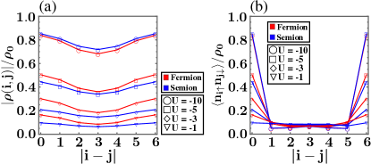
Figure 7: (a) Absolute value of the two-body reduced density matrix $\rho(i,j)$ and (b) the density-density correlation function $\langle n_{i\uparrow}n_{j\downarrow}\rangle$ as functions of the distance $|i-j|$. Each are normalized by the density $\rho_{0}\equiv N/(2N_{x}N_{y})$. The system size is $N_{x}\times N_{y}=6\times 6$ and the particle number is $N=6$. We set $(\eta_{x},\eta_{y})=(\pi/4,0)$ and $(\eta_{x},\eta_{y})=(0,0)$ for semions and fermions, respectively.

Let us now discuss the presence of off-diagonal long-range order. Focusing on the systems at $U<0$, we plot in Fig. 7(a) the two-body reduced density matrix $|\rho(i,j)|/\rho_{0}$, where $\rho_{0}=N/(2N_{x}N_{y})=1/12$ is the density. We set $i=(i_{x},i_{y})=(1,2)$ and change the other site as $j=(1,2),(2,2),(3,2),\ldots,(6,2)$, corresponding to $|j-i|=0,1,2,\ldots,6$. The twisted boundary conditions are set as $(\eta_{x},\eta_{y})=(\pi/4,0)$ to obtain a unique ground state. As a sanity check for translational symmetry, we confirm that the values of $|\rho(i,j)|$ at $U=-1$ with $i=(5,3)$ and $j=(5,3),(6,3),\ldots$ are in agreement with that in Fig. 7(a). In the figure, we also show the result with the same system but with fermions with $(\eta_{x},\eta_{y})=(0,0)$ as a reference state of the superconductor.

The size of the Cooper pair in the fermionic system, according to mean-field theory, coincides with the inter-particle distance at $U=-2.56$ as shown in Appendix C. Based on this, we show four types of data in Fig. 7(a): the BEC limit ($U=-10$), the BEC regime ($U=-5$), the intermediate regime ($U=-3$), and the BCS regime ($U=-1$). In the BEC limit ($U=-10$), $\rho(i,j)$ for semions and fermions has quantitatively similar structure, demonstrating off-diagonal long-range order of semionic superconductivity. In Fig. 7(b), we plot the density-density correlation function $\langle n_{i\uparrow}n_{j\downarrow}\rangle$ in the same settings as Fig. 7(a). The result for semions at $U=-10$ is almost the same as that for fermions and one can also see $\langle n_{i\uparrow}n_{i\downarrow}\rangle\sim\rho_{0}$ in both data. These are consistent with the expectation that a pair of semions obeys Bose statistics. As the interaction becomes weaker, $\langle n_{i\uparrow}n_{i\downarrow}\rangle$ becomes smaller, implying that the size of the pairs is larger (since the density-density correlation function obeys the normalization condition $\sum_{j}\langle n_{i\uparrow}n_{j\downarrow}\rangle=N_{\uparrow}N_{\downarrow}/(N_{x}N_{y})$ where $N_{\uparrow}$ and $N_{\downarrow}$ are the number of up-spin and down-spin particles, respectively). The calculation of $\langle n_{i\uparrow}n_{j\downarrow}\rangle$ is useful to estimate the size of pairs, although the system size that we can currently access is not large enough to do it quantitatively.

In the BEC ($U=-5$), the intermediate ($U=-3$), and the BCS ($U=-1$) regimes, $\rho(i,j)$ and $\langle n_{i\uparrow}n_{j\downarrow}\rangle$ for semions behave quantitatively similarly to those for fermions. This suggests that a BCS-BEC crossover occurs in the semion superconductor. At $U=-5,-3,-1$ in Fig. 7(a), $\rho(i,j)$ for semions is always smaller than that for fermions. Noting the absence of superconducting states in noninteracting systems of fermions, one may expect an absence of superconductivity for semions at $U=0$ as well. This is, however, not necessarily correct. For both semions and fermions, the size of a pair becomes large as $U$ approaches zero and therefore the influence of finite-size effects becomes non-negligible. Much larger systems will be necessary to investigate the presence of superconductivity for semions at $U=0$.

IV Conclusion

In this paper, we have constructed a formulation that allows for the Hubbard model of spinful anyons with any values of the on-site interaction. Virtual splitting of sites, which fixes the way opposing spins pass each other on a site, allows for double-spin occupancy. Using this model, we have investigated the emergence of superconductivity for interacting semions. Off-diagonal long range order is numerically confirmed in the strong interaction regime. Our numerical results also suggest that a BCS-BEC crossover occurs in semionic systems. Recently, density-dependent gauge potentials have been realized in cold atoms [47, 48, 49, 50]. We believe that our findings will be useful for further explorations in the physics of semions.

Appendix A Hopping phases and virtual splitting

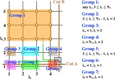
Figure 8: Sketch of a $4\times 5$ lattice. The sites are divided into seven groups.

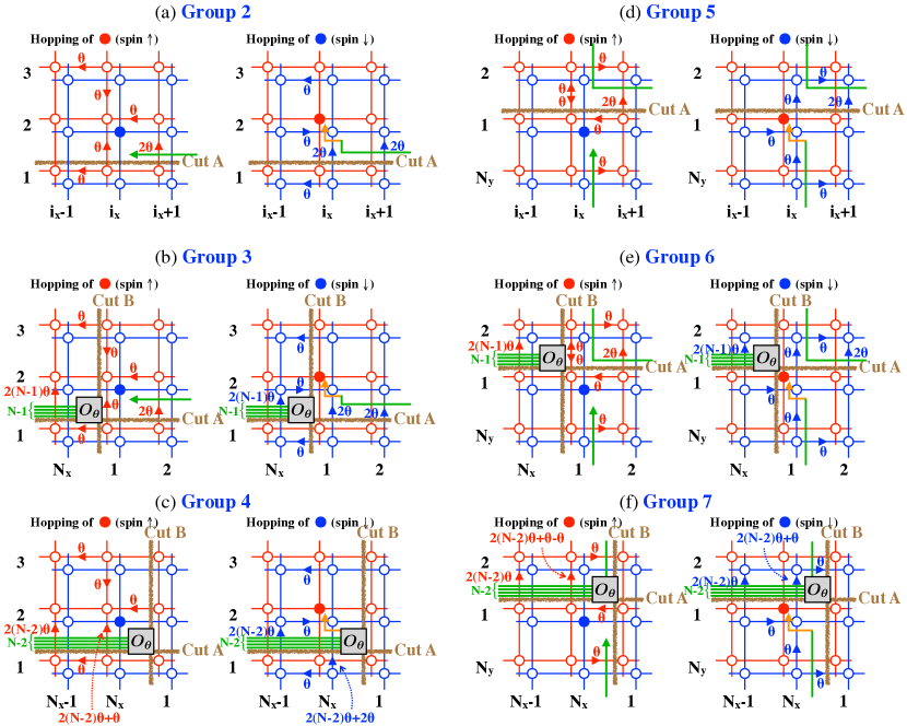
Figure 9: The same as Fig. 5 but for the other groups shown in Fig. 8. (Figure 5 corresponds to Group 1.) We here do not show the phase factors given by $W_{ij\alpha}$, i.e., the plaquette with $O_{\theta}$ has the additional flux $-2\theta$ [see Eq. (9)] other than the sum of the written phases.

In this section, we show that the rules of $\theta_{ij\alpha}$ and $W_{ij\alpha}$ defined in the main text describe virtual splitting. As shown in Fig. 8, we first divide the sites of the system into seven groups and then calculate the hopping phases for each case in Fig. 9 as we did in Fig. 5. For all cases, the sum of the hopping phases along each plaquette matches with the virtual splitting. For simplicity, we impose some conditions of the configuration of the other $N-2$ particles out of the figure without loss of generality [e.g. there are no particles at $i_{x}=N_{x}$ in Fig. 9(b)].

Appendix B Effective Hamiltonian for fermions at $U\ll-1$

Let us rewrite the Hamiltonian in Eq. (10) for $\theta/\pi=1$ (fermions) as $H=H_{\text{kin}}+H_{\text{int}}$ with

$$H_{\text{kin}}=-t\sum_{\langle ij\rangle,\alpha}f^{\dagger}_{i\alpha}f_{j\alpha},$$ (20)

$$H_{\text{int}}=U\sum_{i}\hat{N}_{i\uparrow}\hat{N}_{i\downarrow},$$ (21)

where $f^{\dagger}_{i\alpha}$ is the fermion operator and $\hat{N}_{i\alpha}=f^{\dagger}_{i\alpha}f_{i\alpha}$. To see the expression of $H^{\prime}=PH_{\text{kin}}Q\frac{1}{E_{0}-H_{\text{int}}}QH_{\text{kin}}P$, we consider a two-body state:

$$PH_{\text{kin}}\frac{1}{E_{0}-H_{\text{int}}}H_{\text{kin}}f^{\dagger}_{j\uparrow}f^{\dagger}_{j\downarrow}\ket{0}$$

$$= PH_{\text{kin}}\frac{-t}{U}\sum_{i}\left(f^{\dagger}_{i\uparrow}f^{\dagger}_{j\downarrow}-f^{\dagger}_{i\downarrow}f^{\dagger}_{j\uparrow}\right)\ket{0}$$

$$= \frac{2t^{2}}{U}\sum_{i}\left(f^{\dagger}_{j\uparrow}f^{\dagger}_{j\downarrow}+f^{\dagger}_{i\uparrow}f^{\dagger}_{i\downarrow}\right)\ket{0},$$ (22)

where $\sum_{i}$ indicates the summation over the four nearest sites of $j$. We have $[f^{\dagger}_{i\uparrow}f^{\dagger}_{i\downarrow},f_{j\uparrow}f_{j\downarrow}]=\left(1-\left(N_{i\uparrow}-N_{i\downarrow}\right)\right)\delta_{ij}$ and $P\left(N_{i\uparrow}-N_{i\downarrow}\right)P=0$. Thus, the effective Hamiltonian $H^{\prime}$ is given by

$$H^{\prime}=\frac{2t^{2}}{U}\sum_{\langle ij\rangle}b^{\dagger}_{i}b_{j}+\frac{8t^{2}}{U}\sum_{i}b^{\dagger}_{i}b_{i},$$ (23)

where $b_{i}^{\dagger}$ is the creation operator for a hard-core boson. The twisted boundary conditions for $H^{\prime}$ are given by $(\eta^{\prime}_{x},\eta_{y}^{\prime})=(2\eta_{x},2\eta_{y})$, where $(\eta_{x},\eta_{y})$ is the angles for fermions in the original Hamiltonian. The effective Hamiltonian for semions could be derived using a similar argument, albeit with a modification of the boundary conditions, as discussed in the main text.

Appendix C BCS-BEC crossover

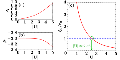
Figure 10: (a) Order parameter $\Delta$, (b) chemical potential $\mu$, and (c) the ratio of the size of the Cooper pair $\xi_{0}$ to the inter-particle distance $r_{0}$ as functions of the Hubbard interaction $|U|$. (c) The dashed line represents $\xi_{0}=r_{0}$. The green circle at $|U|\approx 2.56$ indicates the intersection point.

The Hamiltonian in Eq. (10) for $\theta/\pi=1$ reproduces the standard Hubbard model of fermions. In this section, We calculate the value of $U$ for which the BCS-BEC crossover occurs in the fermionic system.

Assuming $U<0$, we rewrite the Hamiltonian in the reciprocal space as $H=H_{\text{kin}}+V$ with

$$H_{\text{kin}}=\sum_{\bm{k}}\epsilon_{\bm{k}}\hat{N}_{\bm{k}},$$ (24)

$$V=\frac{-|U|}{N_{x}N_{y}}\sum_{\bm{k}_{1},\bm{k}_{2},\bm{k}_{1}^{\prime},\bm{k}_{2}^{\prime}}\delta_{\bm{k}_{1}+\bm{k}_{2},\bm{k}_{1}^{\prime}+\bm{k}_{2}^{\prime}}f^{\dagger}_{\bm{k}_{1}\uparrow}f^{\dagger}_{\bm{k}_{2}\downarrow}f_{\bm{k}_{2}^{\prime}\downarrow}f_{\bm{k}_{1}^{\prime}\uparrow},$$ (25)

where $f^{\dagger}_{\bm{k}\alpha}$ is the fermionic operator, $\hat{N}_{\bm{k}}=f^{\dagger}_{\bm{k}\uparrow}f_{\bm{k}\uparrow}+f^{\dagger}_{\bm{k}\downarrow}f_{\bm{k}\downarrow}$, and $\epsilon_{\bm{k}}=-2t\big{(}\cos(k_{x}a)+\cos(k_{y}a)\big{)}$ with $t=1$. Here we explicitly write the lattice constant $a$. The number of sites is $N_{x}\times N_{y}$. With the condition $\bm{k}_{1}+\bm{k}_{2}=0$, we modify the interaction as

$$V=\sum_{\bm{k},\bm{k}^{\prime}}V(\bm{k},\bm{k}^{\prime})f^{\dagger}_{\bm{k}\uparrow}f^{\dagger}_{-\bm{k}\downarrow}f_{-\bm{k}^{\prime}\downarrow}f_{\bm{k}^{\prime}\uparrow},$$ (26)

where $V(\bm{k},\bm{k}^{\prime})=-|U|/(N_{x}N_{y})$. Now we consider the gap equation at $T=0$:

$$\Delta_{\bm{k}}=-\sum_{\bm{k}^{\prime}}V(\bm{k},\bm{k}^{\prime})\frac{\Delta_{\bm{k}^{\prime}}}{2E_{\bm{k}^{\prime}}},$$ (27)

where $\Delta_{\bm{k}}$ is the order parameter and $E_{\bm{k}}=\sqrt{(\epsilon_{\bm{k}}-\mu)^{2}+\Delta_{\bm{k}}^{2}}$. Since the particle number is fixed in our model, we choose the chemical potential $\mu$ such that

$$\sum_{\bm{k}}\langle\hat{N}_{\bm{k}}\rangle=\sum_{\bm{k}}(1-(\epsilon_{\bm{k}}-\mu)/E_{\bm{k}})=N.$$ (28)

Now we assume $\Delta_{\bm{k}}=\text{const.}\equiv\Delta$. Setting the system parameters as $N_{x}=N_{y}=6$ and $N=6$ and solving Eqs. (27) and (28) simultaneously, we generate Figs. 10(a) and (b) that plot the solutions of $\Delta$ and $\mu$ as functions of $U$.

One expects that the BCS-BEC crossover occurs when the size of the Cooper pair is comparable with the inter-particle distance $r_{0}=a\sqrt{N_{x}N_{y}/N}$. In the continuum limit, the size of the Cooper pair is characterized by

$$\xi_{0}=\frac{\hbar v_{F}}{\pi\Delta}=\frac{\hbar}{\pi\Delta}\sqrt{\frac{2\epsilon_{F}}{m}}.$$ (29)

Substituting $\hbar^{2}/(2m)=ta^{2}$ and $\epsilon_{F}=\mu+4t$ (we here measure the kinetic energy relative to the bottom of the band), we have $\xi_{0}=2a\sqrt{t(\mu+4t)}/(\pi\Delta)$. Figure 10(c) plots the ratio $\xi_{0}/r_{0}$ as a function of $U$. One obtains $\xi_{0}=r_{0}$ at $|U|\approx 2.56$.

——————————

References

- Wu [1984] Y.-S. Wu, Phys. Rev. Lett. 52, 2103 (1984), URL https://link.aps.org/doi/10.1103/PhysRevLett.52.2103.
- Wilczek [1982] F. Wilczek, Phys. Rev. Lett. 49, 957 (1982), URL http://link.aps.org/doi/10.1103/PhysRevLett.49.957.
- Wen [1995] X.-G. Wen, Advances in Physics 44, 405 (1995), eprint http://www.tandfonline.com/doi/pdf/10.1080/00018739500101566, URL http://www.tandfonline.com/doi/abs/10.1080/00018739500101566.
- Tsui et al. [1982] D. C. Tsui, H. L. Stormer, and A. C. Gossard, Phys. Rev. Lett. 48, 1559 (1982), URL http://link.aps.org/doi/10.1103/PhysRevLett.48.1559.
- Arovas et al. [1984] D. Arovas, J. R. Schrieffer, and F. Wilczek, Phys. Rev. Lett. 53, 722 (1984), URL http://link.aps.org/doi/10.1103/PhysRevLett.53.722.
- Moore and Read [1991] G. Moore and N. Read, Nucl. Phys. B 360, 362 (1991), ISSN 0550-3213, URL http://www.sciencedirect.com/science/article/pii/055032139190407O.
- Wen [1991] X. G. Wen, Phys. Rev. Lett. 66, 802 (1991), URL http://link.aps.org/doi/10.1103/PhysRevLett.66.802.
- Laughlin [1983] R. B. Laughlin, Phys. Rev. Lett. 50, 1395 (1983), URL http://link.aps.org/doi/10.1103/PhysRevLett.50.1395.
- Haldane [1985] F. D. M. Haldane, Phys. Rev. Lett. 55, 2095 (1985), URL http://link.aps.org/doi/10.1103/PhysRevLett.55.2095.
- Wen and Niu [1990] X. G. Wen and Q. Niu, Phys. Rev. B 41, 9377 (1990), URL https://link.aps.org/doi/10.1103/PhysRevB.41.9377.
- Einarsson [1990] T. Einarsson, Phys. Rev. Lett. 64, 1995 (1990), URL https://link.aps.org/doi/10.1103/PhysRevLett.64.1995.
- Oshikawa and Senthil [2006] M. Oshikawa and T. Senthil, Phys. Rev. Lett. 96, 060601 (2006), URL https://link.aps.org/doi/10.1103/PhysRevLett.96.060601.
- Sato et al. [2006] M. Sato, M. Kohmoto, and Y.-S. Wu, Phys. Rev. Lett. 97, 010601 (2006), URL https://link.aps.org/doi/10.1103/PhysRevLett.97.010601.
- Oshikawa et al. [2007] M. Oshikawa, Y. B. Kim, K. Shtengel, C. Nayak, and S. Tewari, Annals of Physics 322, 1477 (2007), ISSN 0003-4916, URL http://www.sciencedirect.com/science/article/pii/S0003491606001837.
- Kalmeyer and Laughlin [1987] V. Kalmeyer and R. B. Laughlin, Phys. Rev. Lett. 59, 2095 (1987), URL https://link.aps.org/doi/10.1103/PhysRevLett.59.2095.
- Levin and Wen [2005] M. A. Levin and X.-G. Wen, Phys. Rev. B 71, 045110 (2005), URL http://link.aps.org/doi/10.1103/PhysRevB.71.045110.
- Kitaev [2006] A. Kitaev, Annals of Physics 321, 2 (2006), ISSN 0003-4916, january Special Issue, URL http://www.sciencedirect.com/science/article/pii/S0003491605002381.
- Read and Green [2000] N. Read and D. Green, Phys. Rev. B 61, 10267 (2000), URL http://link.aps.org/doi/10.1103/PhysRevB.61.10267.
- Ivanov [2001] D. A. Ivanov, Phys. Rev. Lett. 86, 268 (2001), URL http://link.aps.org/doi/10.1103/PhysRevLett.86.268.
- Kitaev [2001] A. Y. Kitaev, Physics-Uspekhi 44, 131 (2001), URL https://doi.org/10.1070%2F1063-7869%2F44%2F10s%2Fs29.
- Fu and Kane [2008] L. Fu and C. L. Kane, Phys. Rev. Lett. 100, 096407 (2008), URL https://link.aps.org/doi/10.1103/PhysRevLett.100.096407.
- Qi and Zhang [2011] X.-L. Qi and S.-C. Zhang, Rev. Mod. Phys. 83, 1057 (2011), URL https://link.aps.org/doi/10.1103/RevModPhys.83.1057.
- Schirmer et al. [2022] J. Schirmer, C.-X. Liu, and J. K. Jain, Proceedings of the National Academy of Sciences 119, e2202948119 (2022), eprint https://www.pnas.org/doi/pdf/10.1073/pnas.2202948119, URL https://www.pnas.org/doi/abs/10.1073/pnas.2202948119.
- Kitaev [2003] A. Kitaev, Annals of Physics 303, 2 (2003), ISSN 0003-4916, URL http://www.sciencedirect.com/science/article/pii/S0003491602000180.
- Nayak et al. [2008] C. Nayak, S. H. Simon, A. Stern, M. Freedman, and S. Das Sarma, Rev. Mod. Phys. 80, 1083 (2008), URL http://link.aps.org/doi/10.1103/RevModPhys.80.1083.
- Laughlin [1988] R. B. Laughlin, Phys. Rev. Lett. 61, 379 (1988), URL https://link.aps.org/doi/10.1103/PhysRevLett.61.379.
- Fetter et al. [1989] A. Fetter, C. Hanna, and R. Laughlin, Physical Review B 39, 9679 (1989).
- Chen et al. [1989] Y.-H. Chen, F. Wilczek, E. Witten, and B. I. Halperin, International Journal of Modern Physics B 3, 1001 (1989).
- Wilczek [1990] F. Wilczek, Fractional Statistics and Anyon Superconductivity (World Scientific, 1990), ISBN 9789810200480, URL http://books.google.com/books?id=vFyoQgAACAAJ.
- Halperin et al. [1989] B. I. Halperin, J. March-Russell, and F. Wilczek, Phys. Rev. B 40, 8726 (1989), URL https://link.aps.org/doi/10.1103/PhysRevB.40.8726.
- Kiefl et al. [1990] R. F. Kiefl, J. H. Brewer, I. Affleck, J. F. Carolan, P. Dosanjh, W. N. Hardy, T. Hsu, R. Kadono, J. R. Kempton, S. R. Kreitzman, et al., Phys. Rev. Lett. 64, 2082 (1990), URL https://link.aps.org/doi/10.1103/PhysRevLett.64.2082.
- Spielman et al. [1990] S. Spielman, K. Fesler, C. B. Eom, T. H. Geballe, M. M. Fejer, and A. Kapitulnik, Phys. Rev. Lett. 65, 123 (1990), URL https://link.aps.org/doi/10.1103/PhysRevLett.65.123.
- Girvin and MacDonald [1987] S. M. Girvin and A. H. MacDonald, Phys. Rev. Lett. 58, 1252 (1987), URL http://link.aps.org/doi/10.1103/PhysRevLett.58.1252.
- Jain and Read [1989] J. K. Jain and N. Read, Phys. Rev. B 40, 2723 (1989), URL https://link.aps.org/doi/10.1103/PhysRevB.40.2723.
- Girvin et al. [1990] S. M. Girvin, A. H. MacDonald, M. P. A. Fisher, S.-J. Rey, and J. P. Sethna, Phys. Rev. Lett. 65, 1671 (1990), URL https://link.aps.org/doi/10.1103/PhysRevLett.65.1671.
- Girvin [1992] S. M. Girvin, Progress of Theoretical Physics Supplement 107, 121 (1992), ISSN 0375-9687, eprint https://academic.oup.com/ptps/article-pdf/doi/10.1143/PTPS.107.121/5288574/107-121.pdf, URL https://doi.org/10.1143/PTPS.107.121.
- Leggett, A. J. [1980] Leggett, A. J., J. Phys. Colloques 41, C7 (1980), URL https://doi.org/10.1051/jphyscol:1980704.
- Nozières and Schmitt-Rink [1985] P. Nozières and S. Schmitt-Rink, Journal of Low Temperature Physics 59, 195 (1985), URL https://doi.org/10.1007/BF00683774.
- Wen et al. [1990] X. G. Wen, E. Dagotto, and E. Fradkin, Phys. Rev. B 42, 6110 (1990), URL https://link.aps.org/doi/10.1103/PhysRevB.42.6110.
- Hatsugai et al. [1991a] Y. Hatsugai, M. Kohmoto, and Y.-S. Wu, Phys. Rev. B 43, 2661 (1991a), URL https://link.aps.org/doi/10.1103/PhysRevB.43.2661.
- Hatsugai et al. [1991b] Y. Hatsugai, M. Kohmoto, and Y.-S. Wu, Phys. Rev. B 43, 10761 (1991b), URL https://link.aps.org/doi/10.1103/PhysRevB.43.10761.
- Kallin [1993] C. Kallin, Phys. Rev. B 48, 13742 (1993), URL https://link.aps.org/doi/10.1103/PhysRevB.48.13742.
- Kudo and Hatsugai [2020] K. Kudo and Y. Hatsugai, Phys. Rev. B 102, 125108 (2020), URL https://link.aps.org/doi/10.1103/PhysRevB.102.125108.
- Kudo et al. [2021] K. Kudo, Y. Kuno, and Y. Hatsugai, Phys. Rev. B 104, L241113 (2021), URL https://link.aps.org/doi/10.1103/PhysRevB.104.L241113.
- Kudo and Hatsugai [2022] K. Kudo and Y. Hatsugai (2022), URL https://arxiv.org/abs/2201.07893.
- [46] This feature is consistent with the relations and in the problem of spinless anyons [11, 41].
- Clark et al. [2018] L. W. Clark, B. M. Anderson, L. Feng, A. Gaj, K. Levin, and C. Chin, Phys. Rev. Lett. 121, 030402 (2018), URL https://link.aps.org/doi/10.1103/PhysRevLett.121.030402.
- Görg et al. [2019] F. Görg, K. Sandholzer, J. Minguzzi, R. Desbuquois, M. Messer, and T. Esslinger, Nature Physics 15, 1161 (2019), URL https://doi.org/10.1038/s41567-019-0615-4.
- Schweizer et al. [2019] C. Schweizer, F. Grusdt, M. Berngruber, L. Barbiero, E. Demler, N. Goldman, I. Bloch, and M. Aidelsburger, Nature Physics 15, 1168 (2019), URL https://doi.org/10.1038/s41567-019-0649-7.
- Lienhard et al. [2020] V. Lienhard, P. Scholl, S. Weber, D. Barredo, S. de Léséleuc, R. Bai, N. Lang, M. Fleischhauer, H. P. Büchler, T. Lahaye, et al., Phys. Rev. X 10, 021031 (2020), URL https://link.aps.org/doi/10.1103/PhysRevX.10.021031.
——————————