Torus and polar dust dependence on AGN properties

We present a statistical analysis of the properties of the obscuring material around active galactic nuclei (AGN). This study represents the first of its kind for an ultra-hard X-ray (14–195 keV; Swift/BAT) volume-limited (D${}_{\rm L}<$40 Mpc) sample of 24 Seyfert (Sy) galaxies (BCS₄₀ sample) using high angular resolution infrared data and various torus models: smooth, clumpy and two-phase torus models and clumpy disc$+$wind models. We find that the smooth, clumpy and two-phase torus models (i.e. without including the polar dusty wind component) and disc$+$wind models provide best fits for a comparable number of galaxies, 8/24 (33.3%) and 9/24 (37.5%), respectively. We find that the best-fitted models depend on the hydrogen column density (N${}_{\rm H}^{\rm X-ray}$), which is related to the X-ray (unobscured/obscured) and/or optical (Sy1/Sy2) classification. In particular, smooth, clumpy and two-phase torus models best reproduce the infrared (IR) emission of AGN with relatively high hydrogen column density (median value of log (N${}_{\rm H}^{\rm X-ray}$ cm^-2)=23.5$\pm$0.8; i.e. Sy2). However, clumpy disc$+$wind models provide the best fits to the nuclear IR spectral energy distributions (SEDs) of Sy1/1.8/1.9 (median value of log (N${}_{\rm H}^{\rm X-ray}$ cm^-2)=21.0$\pm$1.0), specifically in the near-IR (NIR) range. The success of the disc$+$wind models in fitting the NIR emission of Sy1 galaxies is due to the combination of adding large graphite grains to the dust composition and self-obscuration effects caused by the wind at intermediate inclinations. In general, we find that the Seyfert galaxies having unfavourable (favourable) conditions, i.e. nuclear hydrogen column density and Eddington ratio, for launching IR dusty polar outflows are best-fitted with smooth, clumpy and two-phase torus (disk$+$wind) models confirming the predictions from simulations. Therefore, our results indicate that the nature of the inner dusty structure in AGN depend on the intrinsic AGN properties.

1 Introduction

Active galactic nuclei (AGN) are powered by accretion of material onto supermassive black holes (SMBHs), which releases energy in the form of radiation and/or mechanical outflows to the interstellar medium (ISM) of the host galaxy. The impact of the energy released by AGN in its surrounding environment has been proposed as a key mechanism responsible for regulating star formation in galaxies (Hopkins & Quataert, 2010). Although they comprise a relatively small fraction of the galaxies in the local universe ($\sim$10%), AGN are now considered to be a short phase ($<$100 Myr; e.g. Hopkins et al. 2005) that might take place in all galaxies (e.g. Hickox et al. 2014).

Nearby Seyfert (Sy) galaxies are intermediate luminosity AGN which are close enough ($\sim$tens of Mpc) to study their nuclear emission and characterize the properties of the nuclear obscurer on $\sim$100 pc scales (at the average angular resolution of 8-10 m-class ground-based telescopes $\sim$0.3″ at 10 $\rm{\mu}$m). The dusty torus/disc is the key piece of the AGN unified model (Antonucci, 1993). Depending on its orientation, it obscures the central engines of type 2 AGN, and provides a direct view of the central engine in the case of type 1 AGN. This nuclear dust absorbs a significant part of the AGN radiation and, then, reprocesses it to emerge in the infrared (IR; e.g. Pier & Krolik 1992).

Early works using direct imaging and interferometric data have found a relatively compact torus ($\sim$0.1-10 pc) in the mid-IR (MIR; $\sim$5–30 $\mu$m; e.g. Jaffe et al. 2004; Packham et al. 2005; Tristram et al. 2007, 2009, 2014; Radomski et al. 2008; Burtscher et al. 2009, 2013; Raban et al. 2009; López-Gonzaga et al. 2016; Leftley et al. 2018). Recently, Atacama Large Millimeter/submillimeter Array (ALMA) observations of the cold dust in Seyfert galaxies have spatially resolved the sub-mm counterpart of the torus (e.g. Gallimore et al. 2016; García-Burillo et al. 2016, 2021; Imanishi et al. 2018; Impellizzeri et al. 2019). García-Burillo et al. (2021) found that the bulk of the nuclear cold dust emission in Sy galaxies is equatorial with a median diameter of $\sim$42 pc. These dusty molecular tori have been also detected in molecular gas observations of Seyfert galaxies and low-luminosity AGNs (e.g. Alonso-Herrero et al. 2018, 2019, 2021; Combes et al. 2019; García-Burillo et al. 2021). These results suggest the multi-phase nature of the torus structure.

Due to the small angular size of the dusty and molecular tori, specially in the IR, 8-10 m-class ground-based telescopes cannot resolve it. Thus, comparing torus models to the observed nuclear IR spectral energy distributions (SEDs) is a powerful tool to constrain the properties of the nuclear dusty structure. Torus models can be broadly grouped in two categories: dynamical (i.e. radiation hydrodynamical and magneto-hydrodynamical simulations; e.g. Wada & Norman 2002; Schartmann et al. 2008; Wada 2012; Dorodnitsyn & Kallman 2017; Kudoh, Wada, & Norman 2020; Takasao, Shuto, & Wada 2022) and static (i.e. radiative transfer models; e.g. Pier & Krolik 1992; Efstathiou & Rowan-Robinson 1995; Fritz et al. 2006; Nenkova et al. 2008a, b; Hönig & Kishimoto 2010, 2017; Stalevski et al. 2012; Stalevski et al. 2016; Siebenmorgen, Heymann, & Efstathiou 2015). The dynamical models include processes such as supernovae and AGN feedback. However, they require large computational times and thus it is more difficult to compare them with observations. On the other hand, static torus models can be easily compared with the observations, assuming various geometries and compositions of the dust (see Ramos Almeida & Ricci 2017; Hönig 2019 for reviews).

For the sake of simplicity, the first geometrical torus models assumed a uniform distribution of the dust (e.g. Pier & Krolik 1992; Fritz et al. 2006). However, pioneering works showed that a clumpy distribution of the dust was necessary to prevent the destruction of grains (Krolik & Begelman, 1988). Therefore, a clumpy formalism has been employed in the majority of torus models (e.g. Nenkova et al. 2008a, b; Hönig & Kishimoto 2010, 2017). Moreover, several hydrodynamical simulations predict that the torus is a multiphase structure (e.g. Wada & Norman 2002; Schartmann et al. 2014) with a combination of smooth and clumpy dust distributions (i.e. two-phase torus models; e.g. Stalevski et al. 2012; Stalevski et al. 2016; Siebenmorgen, Heymann, & Efstathiou 2015).

Since the first torus models were developed, our view of the dusty torus has changed considerably. For instance, recent observations using IR interferometry have motivated a more complex scenario to explain the IR nuclear emission of Seyfert galaxies. Hönig et al. (2013) suggested that a significant fraction of the MIR emission is produced by dust located in the polar direction, whereas the near-infrared (NIR) flux is produced by a clumpy and compact disk (i.e. the dusty torus). Thus, some of the geometrical torus models also include a polar dust component (e.g. Hönig & Kishimoto 2017; hereafter clumpy disc$+$wind models). This polar emission has been detected at small scale (few pc) so far in six sources of the 23 observed using IR interferometry (López-Gonzaga et al., 2016; Leftley et al., 2018; Gámez Rosas et al., 2022; Isbell et al., 2022). In addition, previous works also showed a large scale polar dust component (up to few hundred parsec; e.g. Bock et al. 2000; Radomski et al. 2003; Packham et al. 2005; Asmus et al. 2014, 2019; Alonso-Herrero et al. 2021).

Although the nuclear dust properties of nearby Seyfert galaxies have been extensively studied in the literature, only few works compared SED fits with different torus models to investigate which of them better reproduces the SED of Seyfert galaxies (e.g. González-Martín et al. 2019A, B; hereafter GM19A,19B; Esparza-Arredondo et al. 2019, 2021) and type-1 QSOs (Martínez-Paredes et al., 2021). Given the different assumptions used to build the various available torus models, it is crucial to compare how they fit the observational data. Using Spitzer/IRS spectra ($\sim$5-35 $\mu$m), GM19B found that the clumpy disc$+$wind models (Hönig & Kishimoto, 2017) reproduce well the MIR emission of Sy1, whereas Sy2 are almost equally fitted by clumpy torus models (Nenkova et al. 2008a, b; $\sim$43% of the Sy2s) or clumpy disc$+$wind models ($\sim$40% of the Sy2s). However, this study was limited by the spatial resolution ($\sim$4$\arcsec$) and spectral coverage (5-30 $\mu$m) of Spitzer/IRS. Furthermore, Ramos Almeida et al. (2014) reported that the minimum combination of subarcsecond angular resolution data needed to constrain torus model parameters is N-band spectroscopy (8–13 $\mu$m) and NIR photometry (at least two data-points) when using the clumpy torus models by Nenkova et al. (2008a, b). However, there is a lack of detailed studies comparing different torus models to high angular resolution NIR-to-MIR data of Sy galaxies.

In this work, we investigate for the first time how various geometrical torus models (i.e. smooth, clumpy, two-phases) and disk$+$wind models fit the nuclear IR ($\sim$1-30 $\mu$m) SED of the ultra-hard X-ray volume-limited sample of Sy galaxies (BCS₄₀ sample) presented in García-Bernete et al. (2016). This will allow us to better understand the geometry, chemical composition, grain sizes and distribution of the nuclear dust. In addition, this will help to test the validity of the various torus models.

The paper is organized as follows. Section 2 describes the sample selection. Section 3 gives a summary of the models used throughout this paper. The nuclear IR SED modelling is presented in Section 4. The main results are included in Section 5 and discussed in Section 6. Finally, in Section 7 we summarize the main conclusions of this work.

Table 1: Main properties of the BCS₄₀ sample.

Name	R.A.	Dec.	DL	Spatial	Sy	log (NH)	log (L${}_{\rm int}^{\rm X-ray}$)	log (MBH/M☉)	log ($\lambda_{\rm Edd}$)
	(J2000)	(J2000)	(Mpc)	scale	type	(cm-2)	(erg s-1)
				(pc/arcsec)
(1)	(2)	(3)	(4)	(5)	(6)	(7)	(8)	(9)	(10)
NGC 1365	03h33m36.4s	-36d08m25s	21.5	103	1.8	22.21	42.32	7.92 (a)	-2.44
NGC 2110	05h52m11.4s	-07d27m22s	32.4	155	2.0	22.94	42.69	9.25 (b)	-3.40
ESO 005-G004	06h05m41.6s	-86d37m55s	24.1	116	2.0	24.34	42.78	6.98 (c)	-1.04
NGC 2992	09h45m42.0s	-14d19m35s	34.4	164	1.9	21.72	42.00	5.42 (b)	-0.26
MCG-05-23-016	09h47m40.1s	-30h56m55s	35.8	171	2.0	22.18	43.20	7.98 (a)	-1.62
NGC 3081	09h59m29.5s	-22d49m35s	34.5	164	2.0	23.91	42.72	8.41 (b)	-2.53
NGC 3227	10h23m30.6s	+19d51m54s	20.4	98	1.5	20.95	42.10	6.62 (b)	-1.36
NGC 3783	11h39m01.7s	-37d44m19s	36.4	173	1.2	20.49	43.43	7.14 (a)	-0.55
UGC 6728	11h45m16.0s	+79d40m53s	32.1	153	1.2	20.00	41.80	5.32 (b)	-0.36
NGC 4051	12h03m09.6s	+44d31m53s	12.9	62	1.2	20.00	41.33	5.60 (b)	-1.11
NGC 4138	12h09m29.8s	+43d41m07s	17.7	85	1.9	22.89	41.23	7.30 (b)	-2.91
NGC 4151	12h10m32.6s	+39d24m21s	20.0	96	1.5	22.71	42.31	7.43 (a)	-1.96
NGC 4388*	12h25m46.7s	+12d39m44s	17.0	82	2.0	23.52	43.05	6.99 (b)	-0.78
NGC 4395	12h25m48.8s	+33d32m49s	3.84	19	1.8	21.04	40.50	4.88 (a)	-1.22
NGC 4945	13h05m27.5s	-49d28m06s	4.36	21	2.0	24.80	42.69	7.78 (a)	-1.93
NGC 5128/CenA	13h25m27.6s	-43d01m09s	4.28	21	2.0	23.02	42.39	7.94 (a)	-2.39
MCG-06-30-015	13h35m53.7s	-34d17m44s	26.8	128	1.2	20.85	42.74	7.42 (a)	-1.52
NGC 5506	14h13m14.9s	-03d12m27s	30.1	144	1.9	22.44	42.99	8.29 (a)	-2.14
NGC 6300	17h16m59.5s	-62d49m14s	14.0	68	2.0	23.31	41.84	7.01 (a)	-2.01
NGC 6814	19h42n40.6s	-10d19m25s	25.8	123	1.5	20.97	42.31	6.46 (b)	-0.99
NGC 7172	22h02m01.9s	-31d52m11s	37.9	180	2.0	22.91	42.76	8.45 (b)	-2.53
NGC 7213	22h09m16.3s	-47d10m00s	25.1	120	1.5	20.00	41.95	7.37 (c)	-2.26
NGC 7314	22h35m46.2s	-26d03m02s	20.9	100	1.9	21.60	42.33	7.24 (b)	-1.75
NGC 7582	23h18m23.5s	-42d22m14s	22.1	106	2.0	24.33	42.86	7.52 (a)	-1.50

2 Sample selection

Our sample consists of 24 Seyfert galaxies selected from the nine-month catalog (Tueller et al., 2008) observed with Swift/BAT. This sample was previously presented in García-Bernete et al. (2016) (hereafter BAT Complete Seyfert sample at D${}_{L}<$40 Mpc, BCS₄₀ sample). The ultra-hard 14-195 keV band used to select the parent sample is far less sensitive to the effects of obscuration than optical or softer X-ray wavelengths, making this AGN selection one of the least biased for N_H $\rm{<}$10²⁴ cm^-2 to date (see e.g. Winter et al. 2009, 2010; Weaver et al. 2010; Ichikawa et al. 2012; Ricci et al. 2015; Ueda et al. 2015). We selected all the Seyfert galaxies in the nine-month catalog with luminosity distances D${}_{L}<$40 Mpc. We used this distance limit to ensure a resolution element of $\leqslant$50 pc in the MIR, considering the average angular resolution of 8-10 m-class ground-based telescopes ($\sim$0.3″ at 10 $\rm{\mu}$m). The sample contains 8 Sy1 (Sy1, Sy1.2 and Sy1.5), 6 Sy1.8/1.9 and 10 Sy2 galaxies. This sample covers an AGN luminosity range log(L${{}_{\textrm{bol}}}$ erg s^-1)$\sim$41.75-44.75 and X-ray hydrogen column densities of N${}_{\rm H}^{\rm X-ray}\sim$1$\times$10²⁰-6$\times$10²⁴ cm^-2. Note that we use bolometric luminosities derived by using the commonly employed bolometric correction of 20 (L${{}_{\textrm{bol}}}$=20 $\times$ L${{}_{2-10\leavevmode\nobreak\ \textrm{keV}}}$; e.g. Vasudevan & Fabian 2009) at the 2-10 keV luminosities listed in Table 2. The main properties of the BCS₄₀ sample are shown in Table 2.

3 Torus models

We have chosen six models comprising different dust compositions, distributions and geometries (see also González-Martín et al. 2019A and references therein). In Figure 1 we summarize the dust geometries and compositions, sublimation temperatures, and main parameters of each model used in this work. We also present a brief description of the models below:

$\rm{\bullet}$ Smooth torus model by Fritz et al. (2006) (hereafter smooth F06 torus models): The model used a simple toroidal geometry, consisting of a flared disc represented as two concentric spheres having the polar cones removed. These two spheres delimit the inner and the outer torus radius, respectively. For the composition of dust the model considered a standard Galactic mix of 53% silicates and 47% graphite. The silicate and graphite grains have radii of $\rm{a_{g}}$ = 0.025 - 0.25 and $\rm{a_{g}}$ = 0.005 - 0.25 $\rm{\mu m}$, respectively. The parameters of the model are the viewing angle toward the torus, $i$, the half opening angle of the torus, $\sigma$, the exponent of the logarithmic azimuthal and radial density distribution, $\gamma$ and $\beta$, respectively, the ratio between external and internal radii, $\rm{Y=R_{\rm o}/R_{\rm d}}$, and the edge-on optical depth at 9.7 $\mu m$, $\tau_{9.7\mu m}$ (see Table 12 of Appendix A).

$\rm{\bullet}$ Clumpy torus model by Nenkova et al. (2008a, b) (hereafter clumpy N08 torus models): The model used a formalism that accounts for the concentration of dust in clouds, forming a torus-like structure. They assumed spherical dust grains and a standard Galactic mix of 53% silicates and 47% graphite. The parameters of the model are: the view angle toward the torus, $i$, the number of clouds, $N_{0}$, the half opening angle of the torus, $\sigma$, the ratio between external and internal radii, $\rm{Y=R_{\rm o}/R_{\rm d}}$, the slope of the radial density distribution, $q$, and the optical depth of the individual clouds, $\tau_{\nu}$ (see Table 13 of Appendix A).

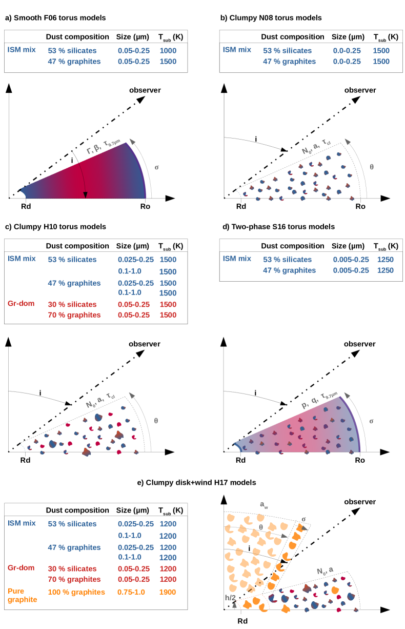
Figure 1: Scheme showing the different dust geometries and compositions of the various torus models used in this work. See Appendix A for further details on the individual model parameters. Note that the clumpy disc H17D models are not represented in this figure. However, the latter models consist of clumpy disc component of the clumpy disc$+$wind H17 models.

$\bullet$ Clumpy toroidal model by Hönig & Kishimoto (2010) (see also Hönig et al., 2006, 2010) (hereafter clumpy H10 torus models): These are radiative transfer models of three-dimensional clumpy dust tori using optically thick dust clouds and a low torus volume filling factor. The majority of the models use a standard ISM dust mixture of graphite (47%) and silicate (53%) dust grains with a classical MRN size distribution (Mathis, Rumpl, & Nordsieck 1977) and a maximum size of 0.25 $\mu$m. By contrast, clumpy H10 torus models also include ISM-like large grains with sizes between 0.1 and 1.0 $\mu$m (i.e. using the same graphite/silicate mixture) and a population of graphite dominated grains (high refractory material), with 70% fraction of graphites (30% silicates) and maximum sizes of 0.25 $\mu$m. The parameters of this library of SEDs are: the viewing angle $i$, the number of clouds along an equatorial line-of-sight $\rm{N_{0}}$, the half-opening angle of the distribution of clouds $\rm{\theta}$, the radial dust-cloud distribution power law index $a$, and the opacity of the clouds $\rm{\tau_{cl}}$. The outer torus radius $\rm{R_{\rm o}}$ is fixed to the inner radius as $\rm{R_{\rm o}=150\,R_{d}}$ (see Table 14 of Appendix A).

$\rm{\bullet}$ Two-phase torus model by Stalevski et al. (2016) (hereafter two-phase S16 torus models): The model used a torus geometry with a two-phase dusty medium, consisting of high-density clumps embedded in a smooth dusty component of low density. The dust chemical composition is set to a mixture of silicate and graphite grains. Model parameters are: the viewing angle toward the observer, $i$, the ratio between the outer and the inner radius of the torus, $Y=\rm{R_{\rm o}/R_{\rm d}}$, the half opening angle of the torus, $\sigma$, the indices that set dust density gradient with the radial $p$ and polar $q$ distribution of dust, and the $9.7\mu m$ average edge-on optical depth, $\tau_{9.7\mu m}$ (see Table 15 of Appendix A).

$\rm{\bullet}$ Clumpy disc and outflow model by Hönig & Kishimoto (2017) (hereafter clumpy disc$+$wind H17 models): The model consists of a clumpy disc plus a polar outflow. The authors used the same dust composition as in the clumpy H10 torus models, but they also included a second population of large pure-graphite grains (0.75-1.0 $\mu$m) which are more resilient than small silicates in hard environments (see e.g. Waxman & Draine 2000; Perna, Lazzati, & Fiore 2003; Schartmann et al. 2008; Lu, Kumar, & Evans 2016; Almeyda et al. 2017; García-González et al. 2017; Hönig & Kishimoto 2017). The parameters for this model are the viewing angle, $i$, and the number of clouds in the equatorial plane, $N_{0}$, the exponent of the radial distribution of clouds in the disc, $a$, the optical depth of individual clouds in the disc, $\tau_{cl}$ (fixed to 50), the index of the dust cloud distribution power-law along the wind, $a_{w}$, the half-opening angle of the wind, $\theta$, the angular width of the hollow wind cone, $\sigma$, and the wind-to-disc ratio, $f_{wd}$ (defines the ratio between the number of clouds along the cone and $N_{0}$) (see Table 16 of Appendix A). Note that this model assumes a fixed clouds radius (R${}_{\rm cl}=$0.035$\times$r_sub).

$\rm{\bullet}$ Clumpy disc by Hönig & Kishimoto (2017) (hereafter clumpy disc H17D models): The model consists of clumpy disc component of the previously described clumpy disc$+$wind H17 models (i.e. removing the wind component). Thus, the authors used the same dust grain composition and dust sublimation formalism as in the clumpy disc$+$wind H17 models (see text above and Table 16 of Appendix A). Note that we include this model to further investigate the impact of the pure-graphite polar dust component on the fits (see Section 6.3).

It is worth noting that the main differences between the various models employed in this study are: a) nuclear dust geometry (i.e. torus, disc+wind), b) dust distribution (i.e. smooth, clumpy or two-phase) and c) dust composition and the treatment of the sublimation temperature of the dust grains. In particular, clumpy disc$+$wind H17 models are significantly different from the other torus models described above, both in the dust geometry and composition (see Section 3). Hönig & Kishimoto (2017) proposed that a polar dusty outflow is launched near the dust sublimation zone and thus the polar dust composition should be similar to the dust in the inner regions of the disc (see Hönig & Kishimoto 2017; Isbell et al. 2021). Therefore, they only included a population of large pure-graphite grains in the polar dust component assuming that it is swept-up dust from the inner wall of the torus/disc where silicate grains are destroyed by the intense emission from the AGN. In contrast, they included both silicate and graphite grains in the torus/disc component. To account for the different dust compositions, Hönig & Kishimoto (2017) used a physically motivated dust sublimation model considering that larger grains are heated less efficiently than smaller grains. This leads to various grain radial layers (species and sizes), where large graphite grains are hotter and closer to the AGN (e.g. Schartmann et al. 2008). Note that this sublimation temperature treatment is not taken into account in the other torus models considered here (e.g. Nenkova et al. 2008a, b; Hönig & Kishimoto 2010; Stalevski et al. 2016), although the smooth F06 torus models use different sublimation temperatures (T${}_{\rm sub}^{\rm silicates}$=1000 K and T${}_{\rm sub}^{\rm graphites}$=1500 K). Note that for simplicity throughout this work we will use the term torus models to refer to the smooth, clumpy and two-phases torus models (i.e. those models that do not include the dusty polar component).

4 SED fitting with torus models

4.1 Accretion disc contribution

The subarcsecond resolution NIR fluxes of type 2 AGN are dominated by emission from hot AGN-heated dust with very little or no contribution from the accretion disc. However, another contribution to the NIR emission can be stellar emission from the host galaxy. To separate, as much as possible, the nuclear NIR emission from the stellar emission the highest possible spatial resolution is required (see e.g. Alonso-Herrero et al. 1998, 2003). Then, we assume that the flux contained in the scaled PSF (i.e. scaled PSF-star to the peak of the galaxy emission at different percentages; e.g. García-Bernete et al. 2015, 2016; GB19 and references therein) corresponds to the unresolved component and it is practically uncontaminated by star formation.

In the case of type 1 AGNs, the NIR emission is mainly produced by very hot dust and the direct emission from the accretion disc of the AGN (see e.g. Hernán-Caballero et al. 2016, GB19, Landt et al. 2019 and references therein). To quantify the contribution from the accretion disc to the nuclear NIR emission, we followed the same procedure as described in Hernán-Caballero et al. (2016) using a semi-empirical model consisting of a template for the accretion disc and two blackbodies to fit the optical and NIR emission of each galaxy individually (see GB19). In GB19 we found that the accretion disc contribution to the nuclear IR SEDs ($\sim$0.4 arcsec) of Sy1s was, on average, 46$\pm$28, 23$\pm$13, and 11$\pm$5% in the J, H, and K bands, respectively. Therefore, we subtracted the accretion disc component in the NIR range of each source prior to fitting the nuclear IR SEDs with the various torus models (see GB19 for further details).

Table 2: Summary of models producing the best fit for each galaxy.

Object	Best model–HR	Best model–LR
Sy1 galaxies
MCG-06-30-015	H17	H17
NGC3227	H17 (H17D)	H17 (H17D)
NGC3783	H17	H17
NGC4051	…	…
NGC4151	H17	H17
NGC6814	H17	H17
NGC7213	H17D	H17D
UGC6728	H17/H17D (H10)	H17/H17D
Sy1.8/1.9 galaxies
NGC1365	H17	H17
NGC2992	H17	H17
NGC4138	H17/H17D (H10)	H17/H17D
NGC4395	…	…
NGC5506	H17	H17
NGC7314	H17	H17
Sy2 galaxies
ESO005-G004	…	…
MCG-05-23-016	H17D (S16/H10/H17/N08)	H17D/H10 (H17)
NGC2110	H17D (H17/H10/N08)	H17D (H17/H10)
NGC3081	S16 (H17D/F06/H10/H17/N08)	H17D/H10/S16/N08 (H17)
NGC4388	H10	H10
NGC4945	N08 (F06/H10/S16)	N08/S16 (H10/F06)
NGC5128	H10 (F06/H17/S16/H17D)	H10/H17D/H17/S16 (F06)
NGC6300	…	…
NGC7172	…	…
NGC7582	F06 (H17/S16/H17D)	F06/S16 (H17D/H17/H10)

4.2 SED fitting procedure

Using the torus models described in Section 3 and XSPEC (Arnaud, 1996), which is a command-driven and interactive spectral-fitting program within the HEASOFT software, we fitted all the nuclear NIR-to-MIR SEDs of our sample of Seyfert galaxies. XSPEC provides an easy way to incorporate new models using additive tables together with a wide range of tools to perform spectral fittings to the data.

To construct high angular resolution NIR-to-MIR SEDs for the whole sample we compiled the highest angular resolution IR ($\sim$1-30 $\mu$m) nuclear fluxes available from the literature. The published MIR photometry and N-band spectroscopy (7.5–13 $\mu$m) used in this work was obtained with 8-10 m-class ground-based telescopes and different instruments (e.g. Gran Telescopio CANARIAS/CanariCam, Very Large Telescope/VISIR, Gemini/T-ReCS and MICHELLE). The nuclear NIR fluxes are from both ground- and space-based (i.e. Hubble Space Telescope; HST) data (see Table 2 of GB19). In this work, we used the nuclear IR SEDs as in GB19 (see e.g. Fig. 2 and Appendix A). We converted the N-band spectra and IR photometric data into XSPEC format using the flx2xsp task within HEASOFT.

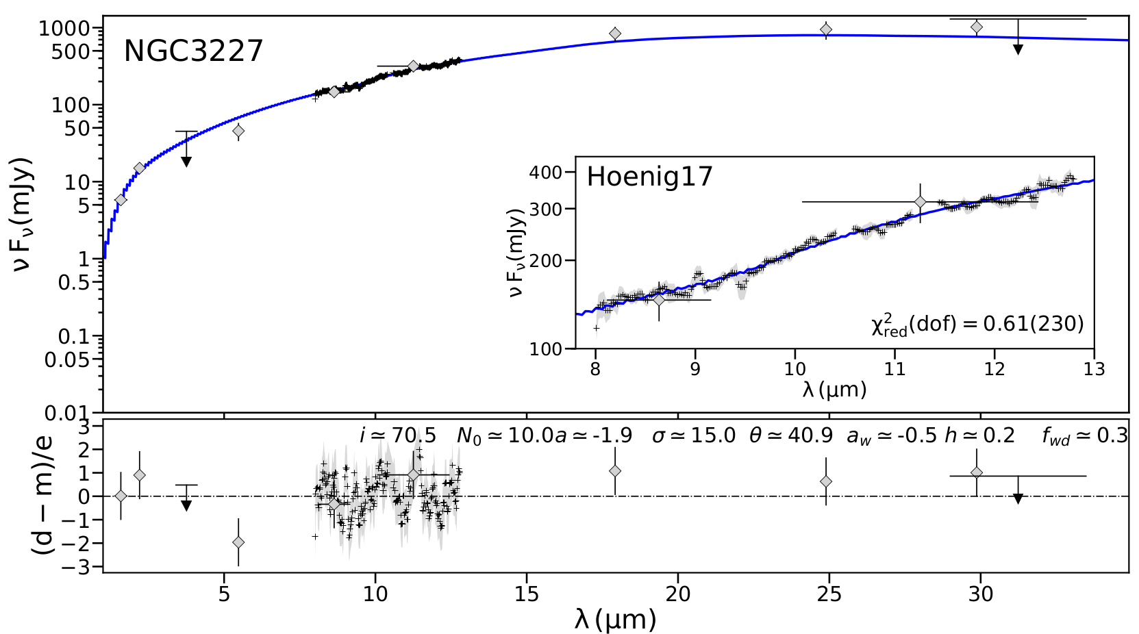
Figure 2: Example of the nuclear IR SED of NGC 3227 fitted with the clumpy disc$+$wind H17 models (top panel) and its residuals (bottom panel). The grey diamonds correspond to the high angular resolution photometric points. The black arrows represent low angular resolution data, which are treated as upper limits. Black crosses correspond to the high angular resolution N-band spectrum. The solid blue line is the best-fitted model.

We masked regions containing narrow spectral features, the 11.3 $\rm{\mu m}$ feature attributed to polycyclic aromatic hydrocarbon molecules (PAHs), and [S IV]$\lambda$10.5$\rm{\mu m}$ and [Ne II]$\lambda$12.8$\rm{\mu m}$ emission lines, to reveal the IR continuum. Note that other weak emission lines are not masked, since they do not affect the fit and that the other PAH emission bands are relatively weak in this sample. Previous studies also showed the importance of including an IR extinction law for fitting the IR SED of Sy galaxies (e.g. Ramos Almeida et al. 2011b; hereafter RA11; Alonso-Herrero et al. 2011; hereafter AH11; Ramos Almeida et al. 2014 & García-Bernete et al. 2019; hereafter GB19). This is especially important for sources with very deep silicate features which generally show prominent dust lanes and/or are hosted in highly inclined galaxies (e.g. AH11, González-Martín et al. 2013). To do so, we use the IR extinction curve of Pei (1992), which is already included as a multiplicative component within XSPEC.

High spatial resolution N-band spectroscopy provides information on the silicate feature around 9.7$\rm{\mu m}$ which is important for the restriction of the model parameters (see e.g. Martínez-Paredes et al. 2020). However, including spectral and photometric data in the fit is not a straightforward task from the statistical point of view. The $\chi^{2}$ statistic method takes every point into account equally so the best fit would tend to match the N-band spectral region over the photometric points. To avoid this, we perform the spectral fitting into two steps. We first fit the photometric data and low spectral resolution N-band spectrum (low-resolution, LR, fit). The LR spectra are computed to match the average bandpass of the photometric data. Then, we compute the 3$\rm{\sigma}$ errors for each parameter, which we use as priors for the SED fitting using the full resolution N-band spectra (high resolution, HR, fit). Note that the same methodology has been used in Martínez-Paredes et al. (2021) for a sample of QSOs.

We compute the $\chi^{2}$ statistics for both the LR and HR fits. We consider the fit to be acceptable if the reduced $\rm{\chi^{2}}$ (for both HR and LR; see e.g. GM19A,19B) is $\rm{\chi^{2}_{red}<2}$. Among them, the best fit is the one providing minimum $\rm{\chi^{2}_{red}}$ and we consider two fits equally good if $\rm{(\chi^{2}_{red}-\chi^{2}_{red,min})<0.5}$. In Appendix A, we present the results of the nuclear IR SED fitting process with the various torus models (see Section 3). Tables 17, 18, and 19 of Appendix A show the results for Sy1, Sy1.8/1.9, and Sy2 galaxies.

To further evaluate the goodness of the fits we use two methods. First, we use a qualitative method for performing a visual inspection of the residuals. To do so, we construct the average residuals using the entire N-band spectra and IR photometry, but excluding the upper limits (i.e. lower angular resolution data). For consistency, we use the same wavelength grid for all photometry (1.6, 2.2, 5.5, 18.0, 25.0 and 30 $\mu$m) employing a quadratic interpolation of nearby values for each galaxy. Secondly, we use the Akaike information criterion (AIC). This method allows an evaluation of the best fit by comparing the minimum $\rm{\chi^{2}_{red}}$ with as comparably good fits those ($\rm{(\chi^{2}_{red}-\chi^{2}_{red,min})<0.5}$). To determine which one is the best fit to the data, we compare the Akaike weights (Emmanoulopoulos et al., 2016) of the models providing acceptable fits ($\epsilon$=W_model1/W_model2). We consider the best fit when $\epsilon$¡0.01, which means that a given fit is, at least, 10 times better than other good fits (see e.g. Martínez-Paredes et al. 2021). Finally, to investigate whether the goodness of the fit depends on the Seyfert type and other AGN properties, we use Fisher’s exact test that is commonly employed for testing for the independence (see Section 5.1). In Table 4 we present the best (and comparably good) fits to the LR and HR SEDs, which are practically the same. Therefore in the following, we only discuss the HR results.

5 Comparison of the various torus models

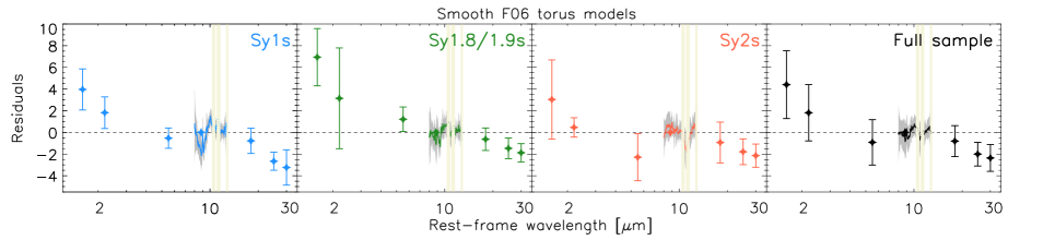
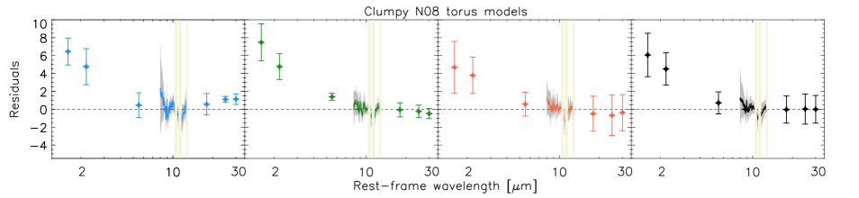
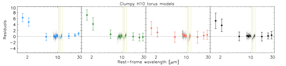
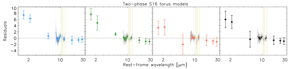
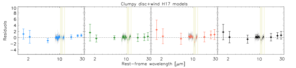
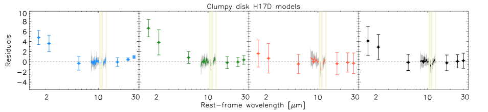
Figure 3: Average residuals (units as in Fig. 2) of the spectral fitting for each torus model used in this work. Blue, green, red and black stars (and solid lines) correspond to Sy1, Sy1.8/1.9, Sy2 and the full sample, respectively. The regions masked in the fitting process are highlighted in beige vertical lines.

5.1 Best model fits

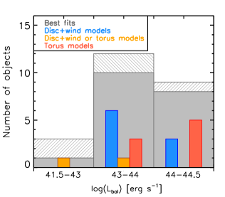
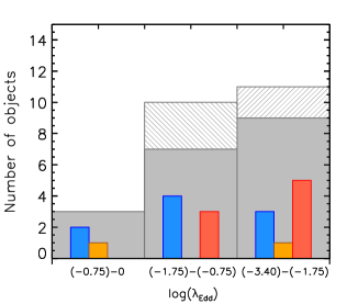
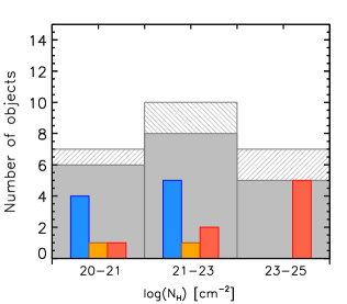
Figure 4: Best fit distributions of the BCS₄₀ sample per bolometric luminosity (left panel), Eddington ratio (central panel) and hydrogen column density (right panel) bin. The grey hatched and filled histograms are the distribution of unfitted and fitted sources. The blue and red filled histograms correspond to sources best fitted by clumpy disc$+$wind H17 models and torus models respectively. The orange filled histograms are sources equally fitted by clumpy disc$+$wind H17 models and torus models.

5.1.1 Average fitting residuals

To determine which are the best suited models for reproducing the entire nuclear NIR-to-MIR SED of the various Sy groups, we first use a qualitative analysis of the average residuals of the spectral fitting. Fig. 3 presents these average residuals of our sample for each of the models considered in this work (see Section 3). The average residuals are computed by grouping the various Seyfert types: from left to right panels of Fig. 3 are Sy1, Sy1.8/1.9, Sy2 and the full sample. From visual inspection of Fig. 3, the average residuals of Sy1/1.8/1.9 indicate a clear excess at NIR emission for smooth, clumpy and two-phase torus models (i.e. torus models). This NIR excess was first reported by Neugebauer et al. (1979) using a sample of quasars, and confirmed by Edelson & Malkan (1986) in Seyfert galaxies. The clumpy disc H17D models generally produce slightly smaller residuals in the IR emission of Sy1 galaxies than other torus models used in this work. However, the models including the polar dust component produce the flattest residuals in the NIR for the entire sample (see Fig. 3).

The N-band spectra are equally well-fitted with most of the models, except for the clumpy N08 torus models and two-phase S16 torus models in the 8–10 $\mu$m range. However, this can be in part due to contamination from the 7.7 $\mu$m PAH band. On the other hand, the clumpy H10 torus models, clumpy disc$+$wind H17 models and clumpy disc H17D models show flatter average fitting residuals for the N-band spectra than the other models. Furthermore, the 18–30 $\mu$m range is generally well reproduced by the various torus models, with the only exception of the smooth F06 torus models, which slightly over-predicts the emission above 20 $\mu$m. Therefore, the clumpy disc$+$wind H17 models produce the best fits in the entire NIR-to-MIR range of the Sy1 galaxies in our sample.

smooth F06 torus models	clumpy N08 torus models	clumpy H10 torus models
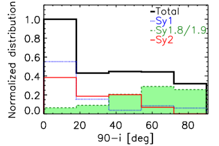
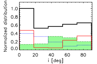
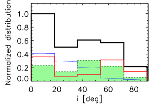
two-phase S16 torus models	clumpy disc$+$wind H17 models

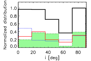
Figure 5: Comparison between the torus/disc inclination combined probability distributions for different models considered here. Blue dotted, green dashed, red solid and black solid lines represent the parameter distributions of Sy1, Sy1.8/1.9, Sy2 and the entire sample, respectively. Note that 90-i_F06=i_N08=i_H10=i_S16=i_H17.

smooth F06 torus models	clumpy N08 torus models	clumpy H10 torus models
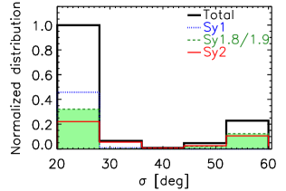
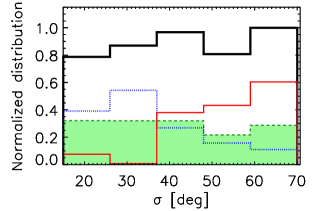
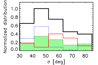
two-phase S16 torus models	clumpy disc$+$wind H17 models

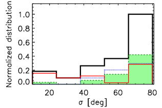
Figure 6: Same as Fig. 5 but for the torus/disc angular width. Note that $\sigma_{\rm H10}$=90-$\theta_{\rm H10}$. In the case of the clumpy disc$+$wind H17 models, the h parameter is the scale height of the dusty disc.

5.1.2 Quantitative methods

In general, all models provide acceptable fits ($\rm{\chi^{2}_{red}<2}$) to the majority (19/24) of the nuclear IR SEDs (see Appendix A). Using the AIC method (see Section 4.2), we find that the fraction of best fits provided by clumpy disc$+$wind and torus models is similar, 37.5 and 33.3% (i.e. 9/24 and 8/24 sources), respectively. Furthermore, 2/24 galaxies (8.3%) are equally fitted by clumpy disc$+$wind or torus models and 5/24 are not well fitted by any of the models used in this work (see Table 4). According to the best fits, the IR SEDs of Sy1 (and Sy1.8/1.9) galaxies are best reproduced by clumpy disc$+$wind H17 models, whereas torus models are best suited to Sy2 galaxies (see Table 8). Using Fisher’s exact test we find that these differences are statistically significant.

Table 3: Summary of the Fisher’s exact test results.

Test	Samples	p-value
(1)	(2)	(3)
Disc$+$Wind best fits	Sy1 vs. Sy2	$<$0.05
Disc$+$Wind best fits	Sy1/1.8/1.9 vs. Sy2	$<$0.05
Disc$+$Wind acceptable fits	Sy1 vs. Sy2	0.37
Disc$+$Wind acceptable fits	Sy1/1.8/1.9 vs. Sy2	0.31
Torus best fits	Sy1 vs. Sy2	$<$0.05
Torus best fits	Sy1/1.8/1.9 vs. Sy2	$<$0.05
Torus acceptable fits	Sy1 vs. Sy2	0.34
Torus acceptable fits	Sy1/1.8/1.9 vs. Sy2	0.12
Unfitted sources	Sy1 vs. Sy2	0.59
Unfitted sources	Sy1/1.8/1.9 vs. Sy2	1.00

The difference in the results for Sy1 and Sy2 galaxies confirms the trend first reported by GM19B using lower spatial resolution Spitzer/IRS MIR spectra of a sample of AGN. However, in this work we confirm them using, for the first time, an ultra-hard X-ray selected sample of Seyferts and high-spatial resolution NIR-to-MIR data that allow us to better isolate the nuclear emission. Moreover, we do not find a clear trend between the models producing the best fits and AGN luminosity or Eddington ratio (see left and central panels of Fig. 4). However, the right panel of Fig. 4 shows that it depends on the line-of-sight hydrogen column density.

In particular, clumpy disc$+$wind H17 models better reproduce the IR emission of AGN with relatively low hydrogen column densities (median value of log (N${}_{\rm H}^{\rm X-ray}$ cm^-2)=21.0$\pm$1.0; i.e. Sy1 and Sy1.8/1.9 galaxies) than torus models. On the other hand, torus models better reproduce the SEDs of AGN with high X-ray hydrogen column densities (median value of log (N${}_{\rm H}^{\rm X-ray}$ cm^-2)=23.5$\pm$0.8; i.e. Sy2s). This is in good agreement with theoretical predictions reported by Venanzi, Hönig, & Williamson (2020), where the authors found that for nuclear column densities of log(N_H cm^-2)$<$23 the IR radiation pressure becomes effective and polar outflows start to emerge (see also AH21).

5.2 Torus model parameters

In this section we investigate the main differences between the derived torus model parameters for the BCS 40 sample using, for the first time, high angular resolution data and various models (see Section 3). Note that we find similar fits using clumpy disc H17D and clumpy H10 torus models. Therefore, in the following, we will not discuss the individual parameters of clumpy disc H17D models.

A general trend is that, even for acceptable fits ($\rm{\chi^{2}_{red}<2}$), the model parameters are not well constrained (see Tables 17, 18, and 19). This result is independent of the torus model, Seyfert type, X-ray absorption along the line of sight or AGN luminosity. Nevertheless, rather than looking at the individual fits (see Appendix A), we focus on the global statistics of the torus model parameters. For this purpose, we derived the combined probability distributions by concatenating together the individual arrays of the parameter probability distributions for all objects in each subgroup (see e.g. GB19). To quantify the differences between the combined probability distributions, we use the Kullback-Leibler divergence (KLD; Kullback & Leibler 1951). This approach takes into account the overall shape of the combined distribution which always has a positive value. The larger the value the greater the difference of the distribution. This value is equal to zero for the case of two identical distributions. RA11 suggested that for values larger than 1 (boldface in Table 20, 21, 22, 23, 24 in Appendix B), two combined distributions may be considered to be significantly different.

Only a few model parameters can be directly compared between the various torus models, for example, the torus/disc inclination angle and its width. According to the KLD test, the differences in the torus/disc inclination angle between Sy subgroups are significant for the smooth F06 torus models, the clumpy H10 torus models and the clumpy disc$+$wind H17 models (see Fig. 5). In general, more edge-on values of the torus/disc inclination are needed for Sy2s than Sy1s. In particular, clumpy disc$+$wind H17 model results show the following trend for the disc inclination: i_Sy1 $<$i_Sy1.8/1.9 $<$i_Sy2. The differences in the angular width of the torus/disc between Sy subgroups are also significant for the various models (see Fig. 6 and Appendix B). In general, the angular widths of the torus of Sy2 galaxies are larger than those of Sy1s (see Fig. 6). The only exception is found for the two-phase S16 torus models, which require a larger angular width of the torus for Sy1/1.8/1.9 than for Sy2 galaxies. Besides, for the clumpy disc$+$wind H17 models, there are no statistically significant differences between the angular width of Sy1 and Sy2 discs. This is likely related with the fact that clumpy disc$+$wind H17 models have relatively “thin” discs and, thus, it would be difficult to find differences between Sy1 and Sy2 discs. Summarizing, our results indicate that generally Sy1 galaxies have tori with smaller angular width and more face-on values of the torus inclination than those of type 2 Seyferts.

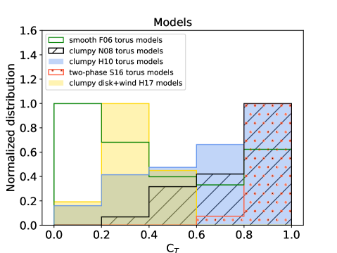
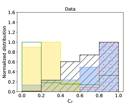
Figure 7: Comparison between the covering factor parameter space. Left panel: combined probability distributions for all the models used in this work. Right panel: combined probability distributions derived for the entire Sy sample using each model.

smooth F06 torus models	clumpy N08 torus models	clumpy H10 torus models
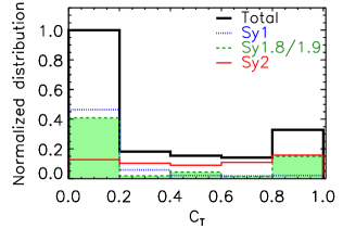
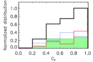
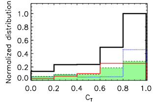
two-phase S16 torus models	clumpy disc$+$wind H17 models

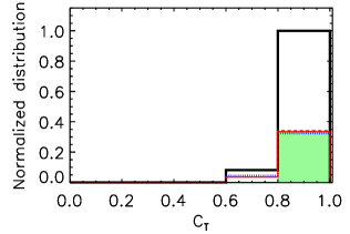
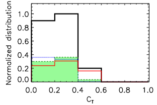
Figure 8: Same as Fig. 5 but for the covering factor.

5.3 Derived torus covering factor, size and mass

5.3.1 The Covering Factor of the nuclear obscuring material

The nuclear obscuration is strongly dependent on the covering factor (C_T) which is defined as the fraction of sky covered by the obscuring material. The covering factor is one of the main elements regulating the intensity of the reprocessed AGN radiation (e.g. RA11, Ramos Almeida & Ricci 2017).

For the various models, C_T can be calculated as:

$$C_{\rm T}=1-\int_{0}^{\pi/2}e^{-\tau_{\nu}\rm(\alpha)}\leavevmode\nobreak\ \cos\alpha\,d\alpha$$ (1)

where $\tau_{\nu}\rm(\alpha)$ is the line-of-sight optical depth, which depends on the azimuthal angle ($\alpha$). The line-of-sight optical depth is computed from the distribution of clouds for clumpy torus models and from the equatorial opacity, and from the density distribution for smooth torus models (see GM19B and references therein).

Since the covering factor is defined as the fraction of the sky at the AGN centre covered by obscuring material, it strongly depends on the torus dust distribution and geometry assumed by the model (see Fig. 7; also GB19B). To further investigate the differences between the various models, we produced the C_T combined probability distributions of the models sampling the entire space of parameters of each model. For example, the clumpy$+$wind H17 model consists of a clumpy dusty disc plus a hollow dusty cone which will naturally produce lower values of the covering factor (C${}_{T}<$0.6; see yellow distribution in left panel of Fig. 7) than a dusty torus with a large range of angular sizes. On the other hand, the two-phase S16 models provide large values of the covering factor (C${}_{T}>$0.6; see red dot distribution in the left panel of Fig. 7). Therefore, caution must be applied when comparing covering factors between various torus models due to the different ranges of parameter space.

In order to compare the C_T probability distributions of the models with those of the observations, we also derived the C_T combined probability distributions (for each model) by concatenating the individual C_T probability distributions of the various galaxies. Indeed, we find that the C_T combined probability distributions of the models and those derived for the entire sample are similar (Fig. 7). For instance, small values of the C_T are derived for the fitted data when using clumpy$+$wind H17 models whereas clumpy H10, clumpy N08 and two-phase S16 models require larger C_T. However, the C_T distributions derived for clumpy$+$wind H17 models tend to have smaller values than the parent distribution. The same applies for the smooth F06 models, whereas the derived C_T distributions for clumpy N08 models favour intermediates C_T values compared with those of the models which peak at larger values. Considering the different C_T ranges covered by the various models, in the following, we have consistently used the same models when comparing covering factors of the Sy groups.

Fig. 8 shows that generally Sy1 have smaller median values of the covering factor than Sy2. According to the KLD test, there are statistically significant differences in the covering factor of Sy1 and Sy2 for the smooth F06 torus models and the clumpy H17 disc$+$wind models (see Appendix B). There is a similar trend, but with less significant (using the KLD test), for the clumpy N08 torus models (see e.g. RA11, AH11, Ichikawa et al. 2015 and GB19). Earlier works using clumpy N08 torus models also showed statistically significant differences between the covering factor of Sy1 and Sy2 galaxies (e.g. RA11, AH11, Ichikawa et al. 2015 and GB19). The lower significance found here might be due to the fact that we are not using priors for the angular width of the torus (based on [O III] data), unlike previous works.

Finally, we find that the covering factor remains broadly constant within the errors for the majority of the models throughout the luminosity range: log(L_bol erg s^-1)$\sim$41.8–45.9. The same applies when using Eddington ratios ($\lambda_{\rm Edd}$: -3.40 to -0.26) instead of the bolometric luminosity.

5.3.2 Torus/disc size and mass

Using the radial extent of the torus/disc (Y=R_o/R_d) and the dust sublimation radius (R_d), we can derive the physical radius of the torus/disc (R_o). The dust sublimation radius also depends on the dust sublimation temperature and the bolometric luminosity. Note that the clumpy H10 torus models and clumpy$+$disc H17 models fixed the Y parameter to a large value for all the SEDs (Y$=$150 and Y$=$500, respectively).

The radius distributions of Sy2 for the smooth F06 torus models and the two-phase S16 models show a tail towards larger tori in comparison with those of Sy1 (see Fig. 9). In particular, in the case of the smooth F06 torus models, we derive median values of the torus size for Sy2 galaxies larger ($\sim$3-5 times) than those of Sy1 and Sy1.8/1.9. Note that using the smooth F06 torus models the radius probability distribution for Sy2 galaxies reaches maximum values of $\sim$30 pc. However, the clumpy N08 torus models do not show statistically significant differences between Sy1 and Sy2 radii. In general, we find relatively compact (1-15 pc) torus radii for all the Seyfert galaxies in our sample (see Fig. 9). Note that we use the term compact torus for those with sizes below the largest resolution element in the MIR for our sample (i.e. $<$50 pc).

smooth F06 torus models	clumpy N08 torus models	two-phase S16 torus models

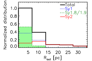
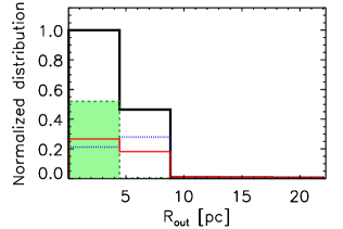
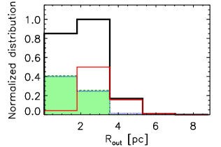
Figure 9: Same as Fig. 5 but for the torus size (R_out).

smooth F06 torus models	clumpy N08 torus models	clumpy H10 torus models
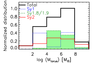
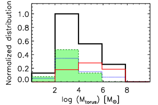
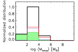
two-phase S16 torus models	clumpy disc$+$wind H17 models

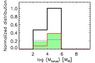
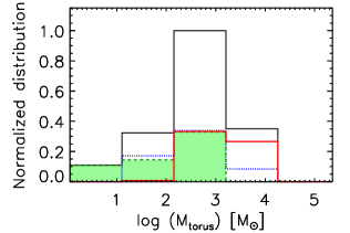
Figure 10: Same as Fig. 5 but for the torus gas mass.

Using the Galactic dust-to-gas ratio (Bohlin, Savage, & Drake, 1978), we can also estimate the torus gas mass associated with the fitted nuclear dusty structure by integrating the density distribution function for each model (see Appendix C, see also GM19B and references therein). We computed the torus mass within the fitted dusty structure volume, thus, it may not be representative of the whole torus gas mass distribution which is traced by the cold gas (see e.g. Hönig 2019 and Section 6.2 for further discussion). We find slightly larger values of the torus/disc gas mass for Sy2 than for Sy1 galaxies, but their differences are generally within the errors (see Fig. 10). The total gas masses of the tori are in the range log(M_torus)$\sim$2-6 M_☉ and, the majority of the models used in this work provide similar values of the total gas mass within the errors (median values of log(M_torus)$\sim$4 M_☉). The exception are the smooth F06 torus (log(M${}_{\rm torus}^{\rm F06}$)=5.6$\pm$1.9 M_☉) and disc$+$wind H17 models (log(M${}_{\rm torus}^{\rm H17}$)=2.6$\pm$0.8 M_☉), for which we find larger gas masses and smaller masses respectively than for the other torus models.

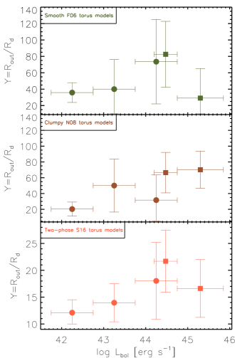
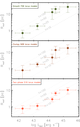
Figure 11: Luminosity dependence of the radial extent of the torus/disc (Y=R_o/R_d; left panels) and of the torus/disc radius (right panels). From top to bottom panels the result for the various models with free Y parameter used in this work (see text for details). The first 3 bins correspond to the Sy galaxies of BCS₄₀ sample. Note that we also include two additional bins of a sample of QSOs with higher bolometric luminosities from Martínez-Paredes et al. (2021).

The derived dusty torus/disc sizes ($\sim$1-15 pc) are similar to those found using MIR imaging and interferometric data (r$<10$ pc; see Section 6.2 for further discussion). However, they are generally smaller than those observed in cold dust by ALMA ($\sim$42 pc; García-Burillo et al. 2021), indicating that larger values of the of the radial extent of the torus/disc (Y) than those covered by the models are needed to match the torus sizes measured in ALMA sub-mm observations at Sy-like luminosities. Indeed, we found larger torus sizes ($\sim$1-34 pc) for the clumpy$+$disc H17 models that use a large value of the radial extent (fixed value of Y=500). Thus, we compare the fitted values of Y with the range covered by the models. The left panel of Fig. 11 shows that the three models compared here do not favour the largest values of Y.

Finally, we also investigate the relation between the bolometric luminosity and the torus/disc size dividing our sample into several luminosity bins (see Fig. 11). In the first bin we include the three sources with log(L_bol erg s^-1)$<$42.75, while the rest of the sample was divided into two bins of equal logarithmic width (1 dex). Note that we also include data from QSOs (i.e. two additional bins from Martínez-Paredes et al. 2021) to expand the range of luminosities beyond our original Sy sample. These authors used the same methodology as here to fit the high angular resolution NIR-to-MIR SEDs of a sample of type 1 QSOs with log(L_bol erg s^-1)$\sim$44.2-45.9. Therefore, these two bins do not include type 2 AGNs. All these models show the same trend throughout the entire luminosity range (log(L_bol erg s^-1)$\sim$41.8–45.9): the higher the luminosity the larger the size (see right panel of Fig. 11). The same applies when using the BH mass instead of the bolometric luminosity. However, we do not find a clear dependence of Y for higher luminosities (see left panel of Fig. 11).

On the other hand, the torus/disc size depends on the Y parameter and dust sublimation radius ($\propto$L${}_{\rm bol}^{1/2}$). Therefore, to further investigate the relationship of the torus size with the luminosity, we compare our results with the expected torus sizes at a given bolometric luminosity and Y parameter (dashed grey lines in right panel of Fig. 11). Considering the almost constant Y values (within the errors) for each luminosity bin and model in the left panel of Fig. 11, the torus size–luminosity correlations might be caused, at least in part, by the sublimation radius dependence with the bolometric luminosity. Futhermore, we find that the derived torus/disc masses also depend on the bolometric luminosities, as expected, given the relation between the torus size and luminosity.

6 Discussion

6.1 The covering factor

It has been suggested that the bolometric luminosity (e.g. Lawrence 1991; Simpson 2005) and Eddington ratio (e.g. Buchner & Bauer 2017; Ricci et al. 2017c) may be the key parameters determining the covering factor. However, according to our results, we do not find a clear dependence of the torus model covering factor with the bolometric luminosity (or the Eddington ratio; see also GB19), although the ranges probed by our sample are relatively reduced (log(L_bol erg s^-1)$\sim$41.8–45.9; $\lambda_{\rm Edd}$: -3.40 to -0.26). This lack of dependence was also reported by Mateos et al. (2016, 2017); Netzer et al. (2016); Stalevski et al. (2016); Lani, Netzer, & Lutz (2017); Ichikawa et al. (2018); GM19B and GB19. Regarding the covering factor, we find that Sy2 galaxies generally have larger values of the covering factor (and angular width of the torus) than Sy1s, for the majority of the models used. This was first reported by RA11 (see also e.g. AH11, Ichikawa et al. 2015 and GB19) but using clumpy N08 torus models only.

Using high-spatial resolution NIR-to-MIR data of an ultra-hard X-ray selected sample of Seyferts, this work confirms that the covering factor of Sy1 and Sy2 galaxies are different. Therefore, our findings indicate that the Seyfert type classification depends not only on the dusty structure inclination but also on the intrinsic differences (e.g. covering factor) of type-1 and type-2 AGN.

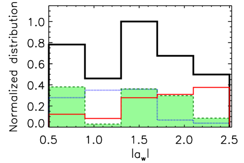
Figure 12: Comparison between the clumpy disc$+$wind H17 model parameters combined probability distributions for the optical classification. Left panel: for the radial dust-cloud distribution power law index (a). Right panel: for the dust-cloud distribution power law along the wind (a_w). Blue dot-dashed, green dashed, and red solid lines represent the parameter distributions of Sy1, Sy1.8/1.9, and Sy2 galaxies, respectively.

6.2 Mid-IR versus sub-mm torus observations

As shown in Section 5.3.2, we find differences on the outer radius of the torus with the AGN type and luminosity, although they depend on the torus models used. In this section we further explore these parameters by comparing the torus/disc size and mass derived from the fitted nuclear IR SED with those measured from IR and sub-mm data (i.e. VLT/SINFONI, NOEMA, and ALMA). For all the models, we derive relatively compact dusty torus/disc sizes ($\sim$1-15 pc). This is in agreement with the torus sizes reported in previous works using the clumpy N08 torus models (see e.g. Ramos Almeida et al. 2009; RA11; AH11; Lira et al. 2013; Ichikawa et al. 2015; Fuller et al. 2016; GB19). The derived torus sizes in this work are of the same order of magnitude as those upper-limit sizes derived from MIR observations. For example, using MIR direct imaging, Packham et al. (2005) and Radomski et al. (2008) found that the MIR size of the torus is less than $\sim$4 pc (diameter) for Circinus and Centaurus A. Furthermore, modelled MIR interferometric data (e.g. Jaffe et al. 2004; Tristram et al. 2007, 2009; Burtscher et al. 2009, 2013; Raban et al. 2009; López-Gonzaga et al. 2016) also show a relatively compact torus of r$<10$ pc. However, recent works using ALMA sub-mm observations of low-luminosity AGN and Seyfert galaxies measure large molecular discs with physical scales (diameters) ranging from 10 to 130 pc, with a typical value of 42 pc (e.g. Alonso-Herrero et al. 2018, 2019, 2021; Combes et al. 2019; García-Burillo et al. 2021). The larger sizes measured in the sub-mm compared to those inferred from IR observations are expected since sub-mm sizes correspond to the colder and, thus, more external material within the torus (e.g. Lopez-Rodriguez et al. 2018; Hönig 2019; Alonso-Herrero et al. 2021; Nikutta et al. 2021).

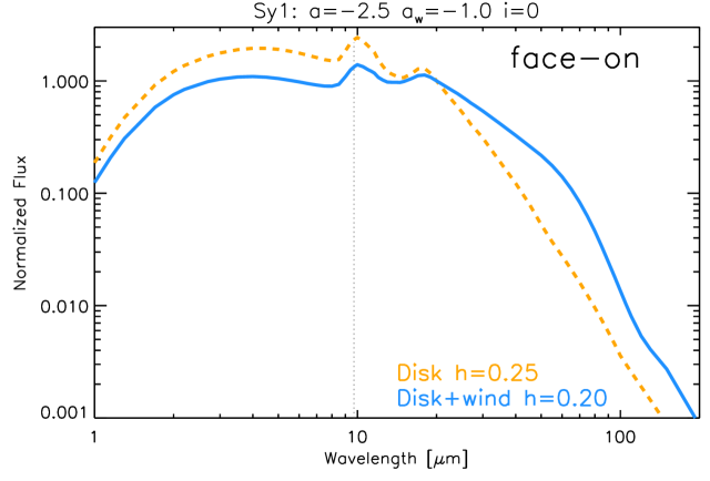
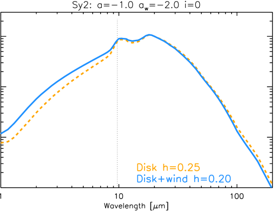
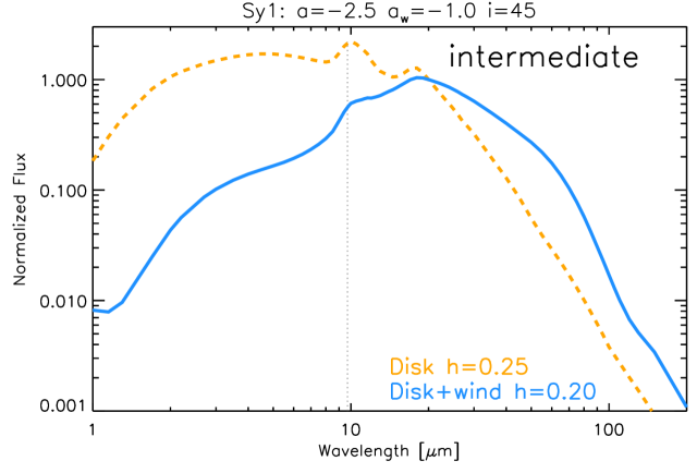
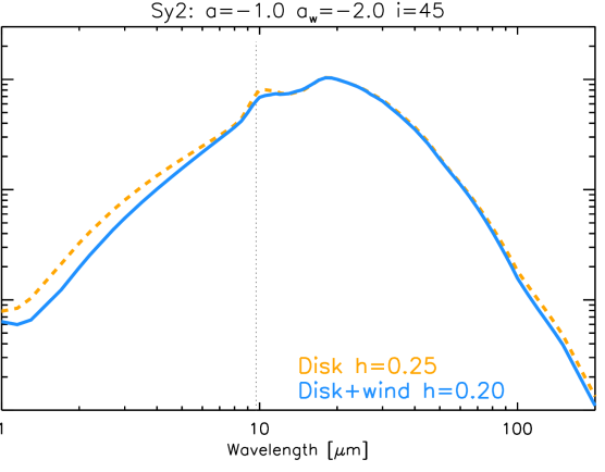
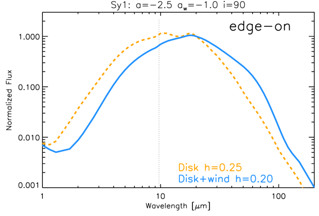
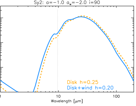
Figure 13: Clumpy disc$+$wind H17 (blue solid lines) and clumpy disc H17 (orange dashed lines) model SEDs (normalized at 20 $\mu$m). Left panel: Sy1 configuration, which consists of a concentrated disc (a=-2.5) and an extended wind (a_w=-1.0). Right panel: Sy2 configuration, which consists of a relatively extended disc (a=-1.0) and a concentrated wind (a_w=-2.0). From top to bottom panels: face-on, intermediate (45^∘) and edge-on values of the inclination angle for the clumpy disk and disk$+$wind dusty structure. Note that all the models use N=7, and the clumpy disc$+$wind H17 models use f_wd=0.6, $\theta$=45^∘ and $\sigma$=10^∘ (see main text for further details on the parameters of the models).

ALMA observations made possible to estimate the molecular gas masses of nearby Seyferts (including a large fraction of the galaxies in this work) and low-luminosity AGN, in the range 10⁵-10⁷ M_⊙ (see e.g. Alonso-Herrero et al. 2018, 2020; Combes et al. 2019; García-Burillo et al. 2021). Using the H₂ 1-0S(1) emission line at 2.12 $\mu$m of a sample of Sy galaxies, Hicks et al. (2009) derived the torus/disc gas masses within the inner 30 pc (radius): M${}_{\rm gas}^{\rm H_{2}}$=0.9–9$\times$10⁶ M_⊙. As expected, the torus masses derived from the fitted nuclear IR SED are relatively smaller ($\sim$10²–10⁶ M_⊙) than those derived from high angular resolution sub-mm data due to the different inferred IR sizes of the torus and those measured in the sub-mm. Therefore, our result is consistent with a temperature-driven stratified disc/torus, where the inner radius is dominated by the hot and warm dust emitting at NIR and MIR wavelengths while the sub-mm observations trace a more extended (and massive) colder component (see also García-Burillo et al., 2021).

6.3 Torus dust composition and geometry

Our findings indicate that torus models better reproduce the NIR-to-MIR emission of AGN with relatively high hydrogen column density (i.e. Sy2s), whereas those of Sy1/Sy1.8/1.9 (with low hydrogen column density) are best fitted by the disc$+$wind H17 model (see Section 4). We also showed that the disc$+$wind dust models improve the spectral fit toward the NIR emission for Sy1/1.8/1.9 galaxies (see also García-González et al., 2017; González-Martín et al., 2019B; Isbell et al., 2021; Martínez-Paredes et al., 2021).

The origin of the NIR bump in the SED remains unclear. Direct emission from the accretion disc of the AGN might be an important contribution of the NIR emission for Sy1 galaxies (e.g. Hernán-Caballero et al. 2016, GB19, Landt et al. 2019 and references therein), but in this work we have remove it from their SEDs. An alternative explanation for the observed NIR excess in Sy1s is an extra contribution of a hot pure-graphite component (T${}_{\rm sub}^{\rm graphites}$¿T${}_{\rm sub}^{\rm silicates}$) heated by the AGN and located in the inner regions of torus (Mor, Netzer, & Elitzur, 2009). García-Bernete et al. (2017) found a tight correlation between the hard X-ray fluxes (Nuclear Spectroscopic Telescope Array; NuSTAR) and the NIR emission of a sample of 24 unobscured type 1 AGN, suggesting that the observed NIR bump is produced by AGN-heated hot dust (T¿T${}_{\rm sub}^{\rm silicates}$).

Clumpy disc$+$wind H17 models predict that the included polar dust (ranging from few pc to tens of pc) mainly contributes to the MIR and sub-mm emission. However, the clumpy disc$+$wind H17 models also include very hot dusty clouds close to the AGN that can reach T$\sim$1900 K (pure-graphite dust; i.e. T¿T${}_{\rm sub}^{\rm silicates}$) whose emission peaks at NIR wavelengths. Thus, in Section 4 we tested if the NIR bump can be explained by including graphite grains. To do so, we repeated the fitting process using only the SEDs of the clumpy disc component of these models (clumpy H17D disc models). The fits have slightly smaller residuals in the NIR range of Sy1 galaxies than other torus models (see Fig. 3). This might be related, at least in part, to the addition of large graphite grains in the dust composition of the disc.

Therefore, it is important to include large pure-graphite grains that are able to survive at high temperatures, and physically motivated dust sublimation models for reproducing, at least in part, the nuclear IR emission of Sy1s. However, the clumpy flared disc from H17D models still produce larger NIR residuals than those of the models including the polar dust component (i.e. clumpy disc$+$wind H17 models). We also note that torus models (i.e. without including the polar dusty wind component) can produce NIR and MIR model images with emission strongly elongated in the polar directions for certain torus parameters (e.g. Lopez-Rodriguez et al., 2018; Nikutta et al., 2021, and references therein). However, Nikutta et al. (2021) found that the observed elongations in IR interferometric data of Seyfert galaxies are difficult to reproduce with a single component torus model (see also Stalevski, Asmus, & Tristram 2017).

6.4 A clumpy disc$+$wind versus clumpy disc IR emission

To further investigate how including the polar dust component modifies the predicted IR emission, we compare the SEDs of the clumpy disc$+$wind H17 models with those of the clumpy disc H17D models. We define two representative set of parameters for Sy1 and Sy2 based on the average values found for each subgroup (see Appendix B). Using the combined probability distributions of the clumpy disc$+$wind H17 models, we find centrally peaked wind components (i.e. ${a_{\rm w}^{\rm Sy2}}<{a_{\rm w}^{\rm Sy1}}$) for Sy2 and less extended disc components (i.e. ${a^{\rm Sy1}}<{a^{\rm Sy2}}$) for Sy1 galaxies (see Fig. 12 and Appendix B). Therefore, we select representative SEDs for Sy1 and Sy2 galaxies using different cloud radial distributions for the disc and the wind, but keeping the other parameters to the same values (N=7, h=0.20, f_wd=0.6, $\theta$=45^∘ and $\sigma$=10^∘; see Table 16 and corresponding Appendix A for a description of the model parameters). In particular, we use two configurations of the radial distributions of the clouds: a) Sy1 configuration with a centrally peaked disc (a=-2.5) and an extended wind (a_w=-1.0); and b) Sy2 configuration with a relatively extended disc (a=-1.0) and a centrally peaked wind (a_w=-2.0).

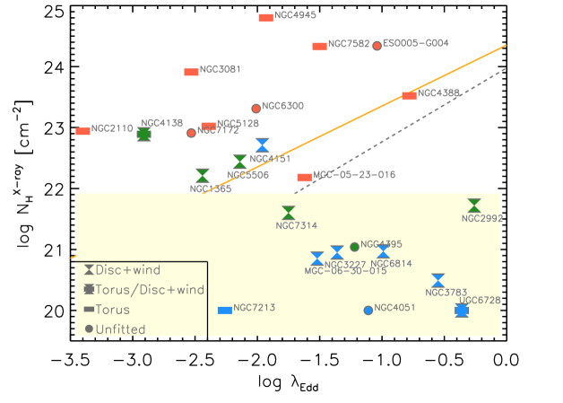
Figure 14: Relation between the X-ray hydrogen column density and the Eddington ratio for the BCS₄₀ sample. Blue, green and red symbols represent Sy1, Sy1.8/1.9 and Sy2, respectively. The yellow shaded region corresponds to the region where X-ray column density might not be representative of the molecular gas column density of the torus (i.e. N${}_{\rm H}^{\rm X-ray}<$10²² cm^-2; García-Burillo et al. 2021). The orange solid line is the limit for IR dusty outflows derived by Venanzi, Hönig, & Williamson (2020) (assuming L_AGN= 2.2$\times$10⁴³ erg s^-1), and the black dashed line represents the blowout limit predicted by Fabian, Vasudevan, & Gandhi (2008). Filled bar and hourglass symbols denote galaxies best fitted by torus and disc$+$wind models, respectively. Filled circles represent those galaxies not fitted by any of the models used in this work.

Fig. 13 shows the clumpy disc$+$wind H17 model SEDs (blue solid lines) of the Sy1 and Sy2 configurations for inclinations of 0, 45 and 90^∘ (i.e. face-on, intermediate inclination and edge-on), and the clumpy disc H17D model SEDs (orange dashed lines) using the same parameters. The SEDs for the Sy2 configuration are practically identical regardless of the addition of the polar dust component (see right panels of Fig. 13), except at intermediate inclinations (i.e. 45^∘) in the NIR and MIR where the self-obscuration of the inner wall of the dusty structure produced by the cone walls is expected to be relevant (see some of the MIR model images presented by Alonso-Herrero et al. 2021). The SEDs of disc$+$wind H17 models are significantly different from those of the clumpy disc H17D models for the Sy1 configuration (see left panels of Fig. 13). The far-IR and sub-mm emission of the Sy1 configuration is strongly enhanced by the extra polar dust component. In addition, the torus angular width can play an important role on the self-obscuration of the inner walls. Furthermore, extra self-obscuration takes place by including a dusty wind component. We find that the strong impact of the self-obscuration from the dusty cone takes place in the NIR and MIR range, especially at intermediate inclinations. The polar dust cone walls can produce moderate self-obscuration up to $\sim$10 $\mu$m at all inclinations (see left panels of Fig. 13; see also Alonso-Herrero et al. 2021). However, the polar dust does not produce strong self-obscuration effects at long wavelengths ($>$20 $\mu$m). Thus, the polar-dust component has a negligible impact in the spectral fit for Sy2 nuclei whereas it produces an enhancement of emission at far-IR and sub-mm wavelengths and an extra self-obscuration at NIR and MIR wavelengths for Sy1 nuclei. This is key to explain the better performance of the disk+wind model for Sy1 nuclei.

6.5 Dependence of the best–fitted model with the AGN properties

Recently, Venanzi, Hönig, & Williamson (2020) presented a semi-analytical model to investigate the simulation of radiatively accelerated dusty winds launched by the AGN. In this model the primary mass reservoir for the outflow is the material within the dusty disc. Their simulations show that the wind and its orientation (polar vs. equatorial) depend on the Eddington ratio, AGN luminosity, and nuclear column density. At relatively high column densities (N${}_{\rm H}>$10²³ cm^-2) the gravity strongly dominates and all the orbits are confined in a compact thick toroidal structure (i.e. the uplift of dusty material is suppressed) for representative values of Sy-like Eddington ratios. At lower values of the column density (N${}_{\rm H}<$10²³ cm^-2) their model predicted that IR dusty outflows can take place above a certain Eddington ratio. From the observational point of view, Alonso-Herrero et al. (2021) found that 7 of 12 Sy galaxies showed Eddington ratios and nuclear N${}_{\rm H}^{\rm ALMA}$ favourable for the launching of the dusty winds, unlike the remaining five galaxies.

Fig. 14 shows the line-of-sight hydrogen column density measured at X-rays (N${}_{\rm H}^{\rm X-ray}$) versus the Eddington ratios for our sample. The black dashed line represents the blowout limit predicted by Fabian, Vasudevan, & Gandhi (2008). The orange solid line is the limit for producing IR dusty outflows derived by Venanzi, Hönig, & Williamson (2020) (assuming L_AGN= 2.2$\times$10⁴³ erg s^-1). Note that we use N${}_{\rm H}^{\rm X-ray}$ measurements which are representative of all the material along a pencil-beam line-of-sight to the accretion disc and, thus, it depends on the viewing direction. Alonso-Herrero et al. (2021) show a similar plot but but using N_H derived from ALMA observations. García-Burillo et al. (2021) compared the hydrogen column densities derived by X-rays and the nuclear integrated values from ALMA for the GATOS sample and found a good agreement between these N_H estimates for obscured Sys (i.e. N${}_{\rm H}^{\rm X-ray}>$10²² cm^-2), whereas the molecular gas column density of the torus probed by ALMA is systematically larger than the N${}_{\rm H}^{\rm X-ray}$ for unobscured Sy galaxies (i.e. N${}_{\rm H}^{\rm X-ray}<$10²² cm^-2). In particular, all Sy1 galaxies in García-Burillo et al. (2021) have N${}_{\rm H}^{\rm ALMA}>$10²² cm^-2. This could be explained as the X-ray absorption in Sys is related with a smaller pc-scale dust-free gas component compared with the scales probed by ALMA ($\sim$10 pc; see e.g. García-Burillo et al. 2021). Therefore, N${}_{\rm H}^{\rm X-ray}$ of Sy1 and Sy1.8/1.9 galaxies might be underestimating the molecular gas column density of the torus. To interpret this plot, we add a yellow shaded region highlighting the region where the X-ray column density might be not representative of the torus structure.

We plot in Fig. 14 galaxies with best fits provided by torus models (i.e. smooth, clumpy, and two-phase torus models) and by disc$+$wind H17 models (see Section 4), using different symbols as shown in the legend. Galaxies with N${}_{\rm H}^{\rm X-ray}>$10²² cm^-2 are located in a region not conducive to launching IR dusty polar outflows, in good agreement with our result that their SEDs are best fitted with torus models. On the other hand, relatively close to the favourable region in the diagram to launching dusty winds, we find a larger number Sys whose SEDs are better fitted with the clumpy disc$+$wind H17 models. Finally, the majority of Sy1 and Sy1.8/1.9 galaxies are located in the the blowout limit region. This might be related, at least in part, to the N${}_{\rm H}^{\rm X-ray}$ measurements. Therefore, this dynamical model is able to broadly explain our main result on the dust configurations and it shows the complexity of the AGN torus.

7 Conclusions

We presented a detailed comparison of the nuclear dust emission of an ultra-hard X-ray (14–195 keV) volume-limited (D${}_{\rm L}<$40 Mpc) sample of 24 Seyfert galaxies to a set of torus models comprising different dust compositions, distributions and geometries. This sample covers AGN luminosity log(L${{}_{\textrm{bol}}^{2-10\leavevmode\nobreak\ \textrm{keV}}}$)$\sim$41.75-44.75 erg s^-1) and Eddington ratio ($\lambda_{\rm Edd}$: -3.40 to -0.26) ranges. We include data from QSOs to expand the range of luminosities (log(L${{}_{\textrm{bol}}^{2-10\leavevmode\nobreak\ \textrm{keV}}}$ erg s^-1)$\sim$44.2-45.9) beyond our original Sy sample. We fitted for the first time the nuclear IR SEDs ($\sim$1-30 $\mu$m) obtained with high angular resolution data with six different torus models to find the model that most closely reproduces the nuclear IR SEDs of type 1 and 2 Seyfert galaxies. Finally, we investigated the relation of the bolometric luminosity, hydrogen column density, and Eddington ratio with different torus parameters. The main results are as follows.

1. The various torus models used in this work provide acceptable fits ($\rm{\chi^{2}_{red}<2}$) to the majority (19/24) of the nuclear IR SEDs. The fraction of best fits provided by smooth, clumpy and two-phases torus models (i.e. those models that do not include the dusty polar component) and disc$+$wind models is practically the same, 33.3 and 37.5% (i.e. 8/24 and 9/24 sources), respectively.
   

2. The disc$+$wind models reproduce better the NIR-to-MIR emission of AGN with relatively low X-ray hydrogen column density (median value of log (N${}_{\rm H}^{\rm X-ray}$ cm^-2)=21.0$\pm$1.0; i.e. Sy1/Sy1.8/1.9), whereas the nuclear IR SED of Sy2 (median value of log (N${}_{\rm H}^{\rm X-ray}$ cm^-2)=23.5$\pm$0.8) are best fitted by smooth, clumpy and two-phases torus models without including the polar dusty wind component.
   

3. The inclusion of large graphite grains with T${}_{\rm sub}\sim$1900 K, in addition to the self-obscuration produced by the polar component at intermediate inclinations (and/or a thick torus) are crucial to reproduce reproduce the observed nuclear NIR and MIR SED of Sy1/1.8/1.9s.
   

4. In general, we find that the Seyfert galaxies having unfavourable (favourable) conditions, i.e. nuclear hydrogen column density and Eddington ratio, for launching IR dusty polar outflows are best-fitted with smooth, clumpy and two-phase torus (disk$+$wind) models confirming the predictions from simulations.
   

Our results indicate that there is a relationship between the choice of model and the hydrogen column density and, thus, the X-ray (unobscured/obscured) and/or optical (Sy1/Sy2) classification. These findings suggest that the torus dusty geometry/grain composition might depend on the amount of nuclear material (N_H) and AGN properties. This work demonstrates the power of the spectral fitting technique to infer the properties of the inner dusty structure in AGN. In the future, the unprecedented combination of high sensitivity and spatial resolution provided by the James Webb Space Telescope (JWST) will be crucial to better understand the nuclear dusty region of AGN using this technique.

Appendix A Torus model parameters and nuclear IR SED fits

Using the various torus models, we fit all the nuclear NIR-to-MIR SEDs in our sample (See Section 4). In Tables 12-16 we present the different torus model parameters. The values of the model parameters fitted to the individual nuclear IR SEDs are reported in Tables 17, 18 and 19. In addition, the individual fits are shown in Figures (A1-A24).

Table 4: Smooth F06 torus model parameters.

Parameter	Symbol	Interval
Inclination angle of the torus	i	[0∘, 90∘]
Width of clouds angular distribution	$\sigma$	[20∘, 60∘]
Exponent of the logarithmic azimuthal	$\Gamma$	[0,6]
density distribution
Exponent of the logarithmic radial	$\beta$	[-1,0]
profile of the density distribution
Radial extent of the torus	Y	[10, 150]
Edge-on optical depth	$\tau_{9.7\mu m}$	[0.1, 10]

Table 5: Clumpy N08 torus model parameters.

Parameter	Symbol	Interval
Radial extent of the torus	Y	[5, 150]
Width of clouds angular distribution	$\sigma$	[15∘, 70∘]
Number of clouds along an equatorial ray	N0	[1, 15]
Index of the radial density profile	q	[0, 3]
Inclination angle of the torus	i	[0∘, 90∘]
Optical depth per single cloud	$\tau_{V}$	[10, 300]

Table 6: Clumpy H10 torus model parameters.

Parameter	Symbol	Interval
Inclination angle of the torus	i	[0∘, 90∘]
Number of clouds along an equatorial line-of-sight	N0	[2.5,10.0]
Half-opening angle of the distribution of clouds	$\theta$	[5∘, 60∘]
Radial dust-cloud distribution power law index	a	[-2,0]
Opacity of the clouds	$\tau_{cl}$	[30, 80]

Table 7: Two-phase S16 torus model parameters.

Parameter	Symbol	Interval
Inclination angle of the torus	i	[0∘, 90∘]
Width of clouds angular distribution	$\sigma$	[10∘, 80∘]
Radial dust density gradient distribution	p	[0,1.5]
Polar dust density gradient distribution	q	[0,1.5]
Radial extent of the torus	Y	[10, 30]
Average edge-on optical depth	$\tau_{9.7\mu m}$	[3, 11]

Table 8: Clumpy disc$+$wind H17 torus model parameters.

Parameter	Symbol	Interval
Inclination angle of the torus	i	[0∘, 90∘]
Number of clouds along an equatorial line-of-sight	N0	[5,10]
Radial dust-cloud distribution power law index	a	[-3.0,-0.5]
Half-opening angle of the wind	$\theta$	[30∘, 45∘]
Angular width of the hollow wind cone	$\sigma$	[7∘, 15∘]
Dust cloud distribution power law along the wind	aw	[-2.5,-0.5]
Scale height of the disc	h	[0.1,0.5]
Wind-to-disc ratio of dust clouds	fwd	[0.15,0.75]

Table 9: Spectral fit results for Type-1 Seyferts.

Obj.	Mod.	$\chi^{2}_{red}$	dof	E(B-V)	Parameters
	F06				$i$	$\sigma$	$\Gamma$	$\beta$	$Y$	$\tau_{9.7\mu m}$
	N08				$i$	$N_{0}$	$\sigma$	$Y$	$q$	$\tau_{v}$
	H10				$i$	$N_{0}$	$\theta$	$a$	$\tau_{cl}$
	S16				$i$	$\sigma$	$p$	$q$	$Y$	$\tau_{9.7\mu m}$
	H17				$i$	$N_{0}$	$a$	$\sigma$	$\theta$	$a_{w}$	$h$	$f_{w}$
	H17D				$i$	$N_{0}$	$a$	$h$
MCG-06-30-015	F06	2.07 / 3.25	420 / 49	0.38$\pm{0.01}$	$<$28.5	$<$20.4	$>$6.0	-0.75$\pm{0.01}$	19.9$\pm{0.3}$	1.01$\pm_{0.02}^{0.01}$
	N08	2.56 / 5.29	420 / 49	0.08$\pm{0.01}$	$>$89.9	$>$14.9	$>$25.2	$<$5.0	$>$2.5	$<$10.0
	H10	1.34 / 2.85	421 / 50	0.27$\pm{0.01}$	51.6$\pm_{0.7}^{0.1}$	$>$9.9	$<$53.6	$<$-1.6	$>$79.5
	S16	1.83 / 4.72	420 / 49	0*	79.9$\pm_{6.5}^{0.5}$	69.1$\pm_{7.4}^{1.3}$	$>$1.5	$>$1.5	$<$10.0	4.04$\pm_{0.02}^{0.17}$
	H17$\bullet$	0.95 / 1.20	418 / 47	0.26$\pm{0.01}$	60.1$\pm_{0.5}^{0.7}$	6.9$\pm_{0.3}^{0.1}$	$<$-3.0	10.0$\pm_{0.3}^{0.4}$	$>$43.0	$>$-0.5	0.28$\pm_{0.01}^{0.03}$	0.30$\pm{0.02}$
	H17D	1.12 / 2.16	422 / 51	0.18$\pm{0.01}$	$>$66.8	$>$9.9	$<$-2.4	$>$0.3
NGC3227	F06	1.35 / 2.76	232 / 33	0.26$\pm_{0.01}^{0.02}$	$<$33.4	$<$20.2	$>$6.0	-0.75$\pm{0.01}$	30.1$\pm_{0.3}^{2.1}$	$>$4.9
	N08	1.38 / 3.02	232 / 33	0.66$\pm_{0.02}^{0.01}$	$<$18.3	1.15$\pm_{0.04}^{0.05}$	$>$47.5	$<$5.2	$>$2.4	$>$296.2
	H10	1.11 / 3.09	233 / 34	0.42$\pm_{0.01}^{0.02}$	$>$46.8	$>$7.5	$<$54.8	$>$-0.8	$>$79.6
	S16	1.39 / 5.27	232 / 33	0*	35.4$\pm_{1.5}^{4.8}$	$<$63.3	1.0$\pm_{0.05}^{0.03}$	$>$0.0	$<$20.1	$<$4.9
	H17$\bullet$	0.61 / 1.26	230 / 31	0.22$\pm_{0.04}^{0.03}$	70.5$\pm{3.2}$	$>$9.1	-1.9$\pm{0.1}$	$>$13.2	$>$36.8	$>$-0.6	$<$0.2	0.3$\pm{0.1}$
	H17D$\bullet$	0.77 / 1.64	234 / 35	0.28$\pm{0.03}$	$>$49.8	6.6$\pm{0.4}$	-1.68$\pm{0.03}$	0.42$\pm{0.02}$
NGC3783	F06	1.23 / 2.42	418 / 28	0.44$\pm{0.01}$	$<$32.7	$<$20.4	$>$0.0	-0.75$\pm{0.01}$	$>$33.1	$>$1.1
	N08	0.89 / 3.95	418 / 28	0.15$\pm_{0.02}^{0.03}$	$>$79.6	5.0$\pm_{0.3}^{0.6}$	36.2$\pm_{5.4}^{11.6}$	$<$5.3	$>$2.4	46.4$\pm_{2.3}^{1.7}$
	H10	0.83 / 3.20	419 / 29	0.25$\pm_{0.03}^{0.02}$	30.0$\pm_{2.1}^{5.0}$	$>$8.9	52.0$\pm_{2.6}^{0.6}$	-0.73$\pm_{0.16}^{0.03}$	$>$79.2
	S16	0.86 / 3.91	418 / 28	0*	$>$68.9	$>$70.2	0.5$\pm_{0.2}^{0.1}$	$>$1.3	$<$12.2	4.5$\pm_{0.4}^{0.1}$
	H17$\bullet$	0.67 / 0.84	416 / 26	0.31$\pm_{0.02}^{0.03}$	$<$28.8	$<$6.7	$<$-2.8	$>$7.8	$>$37.4	-1.0$\pm_{0.1}^{0.2}$	$<$0.1	$>$0.5
	H17D	0.74 / 2.35	420 / 30	0.21$\pm{0.02}$	44.7$\pm_{0.2}^{0.6}$	7.0$\pm_{0.5}^{0.1}$	-1.75$\pm{0.01}$	0.42$\pm_{0.01}^{0.04}$
NGC4051*	F06	1.49 / 2.68	231 / 48	0*	26.6$\pm_{1.3}^{0.5}$	$<$21.1	$>$5.5	-0.75$\pm{0.01}$	$>$26.1	4.8$\pm_{0.2}^{0.3}$
	N08	1.90 / 2.48	231 / 48	0.49$\pm_{0.01}^{0.02}$	$<$19.8	$<$1.0	$>$67.2	$<$5.1	$>$2.5	$>$292.3
	H10	1.38 / 2.38	232 / 49	0.07$\pm{0.04}$	15.0$\pm_{2.3}^{2.9}$	7.8$\pm_{0.3}^{0.5}$	$<$44.4	$>$-0.5	$>$78.8
	S16	1.53 / 3.23	231 / 48	0*	18.5$\pm_{8.6}^{3.0}$	70.0$\pm_{2.0}^{3.1}$	$<$0.6	$<$0.0	$<$14.4	$>$3.7
	H17	1.31 / 2.26	229 / 46	$<$0.04	80.5$\pm_{2.5}^{2.9}$	$>$9.2	$<$-2.9	$>$14.1	$>$43.7	-1.4$\pm{0.1}$	$<$0.1	0.47$\pm_{0.03}^{0.02}$
	H17D	1.28 / 2.06	233 / 50	$<$0.07	30.0$\pm_{9.6}^{3.3}$	5.4$\pm_{0.2}^{0.6}$	-1.5$\pm_{0.1}^{1.2}$	$>$0.7
NGC4151	F06	1.21 / 2.45	162 / 47	0.51$\pm_{0.04}^{0.02}$	$>$67.3	$<$21.5	$>$5.8	-0.75$\pm{0.01}$	30.0$\pm_{0.3}^{0.5}$	$>$1.1
	N08	1.17 / 3.30	162 / 47	0.66$\pm_{0.03}^{0.04}$	$<$27.6	$>$1.0	$>$15.0	$<$6.9	$>$2.3	$>$284.0
	H10	1.16 / 3.22	163 / 48	0.43$\pm_{0.02}^{0.04}$	$>$43.2	7.5$\pm_{0.3}^{0.2}$	$<$57.6	$>$-0.9	$>$78.3
	S16	1.33 / 4.30	162 / 47	$<$0.08	9.9$\pm_{9.2}^{1.2}$	78.1$\pm_{1.4}^{0.7}$	1.0$\pm{0.1}$	$<$0.0	$<$10.5	$<$5.2
	H17$\bullet$	0.29 / 0.71	160 / 45	0.14$\pm{0.03}$	44.8$\pm_{5.0}^{2.2}$	$<$5.6	$<$-3.0	$>$14.4	$>$43.1	-1.56$\pm_{0.02}^{0.03}$	$<$0.1	0.6$\pm_{0.2}^{0.1}$
	H17D	1.00 / 2.37	164 / 49	0.45$\pm_{0.04}^{0.07}$	$>$60.0	$<$5.3	-1.8$\pm_{0.1}^{1.5}$	$>$0.3
NGC6814	F06	1.53 / 2.28	82 / 37	0.16$\pm_{0.02}^{0.01}$	$>$73.0	$<$20.8	$>$6.0	-0.75$\pm{0.01}$	38.9$\pm_{6.6}^{7.7}$	4.1$\pm{0.3}$
	N08	1.94 / 3.77	82 / 37	0.0*	30.0$\pm_{9.2}^{13.3}$	$>$14.3	25.1$\pm_{1.0}^{1.4}$	$<$5.1	$<$0.7	30.0$\pm_{4.6}^{2.6}$
	H10	1.65 / 3.07	83 / 38	0.0*	$<$15.6	7.5$\pm_{0.4}^{0.3}$	45.6$\pm_{1.2}^{1.1}$	-0.53$\pm_{0.03}^{0.02}$	$>$79.2
	S16	1.88 / 3.84	82 / 37	0.0*	40.9$\pm_{3.8}^{2.5}$	50.0$\pm_{2.5}^{2.1}$	$<$0.0	$<$0.1	$<$10.5	4.4$\pm_{0.7}^{0.8}$
	H17$\bullet$	0.81 / 1.19	80 / 35	0.0*	75.0$\pm_{6.4}^{3.9}$	$<$5.9	$<$-2.9	$>$7.0	40.5$\pm_{2.2}^{0.6}$	-1.1$\pm_{0.1}^{0.2}$	$<$0.1	$>$0.6
	H17D	1.54 / 2.29	84 / 39	0.0*	45.1$\pm_{3.0}^{1.2}$	7.0$\pm_{0.9}^{0.1}$	-1.72$\pm_{0.03}^{1.47}$	0.4$\pm_{0.01}^{0.06}$
NGC7213	F06	6.66 / 9.02	418 / 39	1.02$\pm_{0.03}^{0.01}$	$<$0.0	$<$20.3	4.03$\pm_{0.05}^{0.35}$	$>$-0.0	$>$149.9	$<$0.1
	N08	1.05 / 3.09	418 / 39	0.80$\pm_{0.03}^{0.05}$	$<$44.2	2.9$\pm_{0.8}^{1.2}$	$<$16.1	$>$83.0	1.07$\pm_{0.06}^{0.03}$	$>$14.2
	H10	1.23 / 2.85	419 / 40	0.69$\pm_{0.02}^{0.02}$	$<$0.0	$<$2.5	$>$59.9	$>$-0.5	$<$30.1
	S16	8.17 / 10.96	418 / 39	0.05$\pm{0.02}$	30.0$\pm_{0.2}^{1.4}$	$>$79.9	$<$0.0	$>$1.5	$>$30.0	$<$3.0
	H17	1.65 / 2.18	416 / 37	0.46$\pm_{0.01}^{0.02}$	30.0$\pm_{0.3}^{0.1}$	$<$5.0	$>$-1.7	$>$7.3	$<$30.0	-1.0$\pm{0.1}$	$<$0.1	0.45$\pm{0.01}$
	H17D$\bullet$	1.00 / 1.61	420 / 41	0.51$\pm{0.02}$	$<$0.0	$<$5.0	-1.67$\pm_{0.01}^{1.42}$	0.25$\pm{0.01}$
UGC6728	F06	2.72 / 2.54	77 / 42	0.0*	$>$59.6	$>$20.0	$>$0.1	-0.74$\pm_{0.01}^{0.06}$	$<$10.2	1.52$\pm_{0.03}^{0.02}$
	N08	12.11 / 12.13	77 / 42	0.0*	$>$89.7	$>$14.0	34.7$\pm_{1.7}^{0.6}$	$<$5.0	$>$2.5	$<$10.0
	H10$\bullet$	1.35 / 1.40	78 / 43	0.11$\pm{0.01}$	36.0$\pm_{3.7}^{6.2}$	$>$7.4	$<$7.5	$<$-1.9	$>$79.3
	S16	5.10 / 5.33	77 / 42	0.0*	66.5$\pm_{0.9}^{2.3}$	59.6$\pm_{1.8}^{0.7}$	$>$1.5	$>$1.5	$<$10.0	$>$4.0
	H17$\bullet$	1.05 / 0.87	75 / 40	0.23$\pm_{0.01}^{0.02}$	$<$3.2	$>$7.8	$<$-3.0	$>$9.8	36.1$\pm_{1.2}^{2.0}$	-1.6$\pm_{0.1}^{0.2}$	$<$0.1	$>$0.6
	H17D$\bullet$	1.19 / 1.17	79 / 44	0.01$\pm_{0.01}^{0.02}$	44.9$\pm_{2.2}^{0.6}$	$>$9.8	$<$-2.5	$>$0.7

Table 10: Spectral fit results for Type 1.8/1.9 Seyferts.

Obj.	Mod.	$\chi^{2}_{red}$	dof	E(B-V)	Parameters
	F06				$i$	$\sigma$	$\Gamma$	$\beta$	$Y$	$\tau_{9.7\mu m}$
	N08				$i$	$N_{0}$	$\sigma$	$Y$	$q$	$\tau_{v}$
	H10				$i$	$N_{0}$	$\theta$	$a$	$\tau_{cl}$
	S16				$i$	$\sigma$	$p$	$q$	$Y$	$\tau_{9.7\mu m}$
	H17				$i$	$N_{0}$	$a$	$\sigma$	$\theta$	$a_{w}$	$h$	$f_{w}$
	H17D				$i$	$N_{0}$	$a$	$h$
NGC1365	F06	1.13 / 3.43	197 / 38	$<$0.06	$<$33.3	$<$22.4	$>$5.6	$>$-0.1	20.5$\pm_{0.9}^{1.4}$	$>$9.0
	N08	1.06 / 3.07	197 / 38	0.04$\pm_{0.03}^{0.05}$	40.1$\pm_{8.5}^{9.2}$	$>$12.3	26.1$\pm_{1.5}^{1.9}$	5.9$\pm_{0.5}^{0.7}$	$<$0.7	40.0$\pm_{4.1}^{5.3}$
	H10	1.05 / 2.77	198 / 39	0.07$\pm_{0.04}^{0.03}$	$<$21.3	7.5$\pm_{1.6}^{0.4}$	$<$45.6	$>$-0.2	$>$77.3
	S16	1.12 / 3.58	197 / 38	0*	24.6$\pm_{6.9}^{23.0}$	$>$77.9	$<$0.0	$>$1.0	$>$17.2	5.0$\pm_{1.4}^{0.4}$
	H17$\bullet$	0.70 / 0.98	195 / 36	0*	52.9$\pm_{2.6}^{7.6}$	$<$6.8	$<$-3.0	$>$12.6	$>$42.7	-1.58$\pm_{0.05}^{0.28}$	$<$0.1	$>$0.6
	H17D	0.92 / 2.15	199 / 40	$<$0.05	30.2$\pm_{2.0}^{1.3}$	$<$5.1	-1.36$\pm_{0.02}^{1.11}$	$>$0.7
NGC2992	F06	2.18 / 3.96	233 / 38	1.0$\pm_{0.03}^{0.02}$	$<$69.4	$<$20.1	$>$6.0	$>$-0.0	$>$51.8	$>$10.0
	N08	1.25 / 2.36	233 / 38	0.79$\pm{0.03}$	$<$62.9	$>$13.6	17.3$\pm_{0.6}^{1.4}$	14.7$\pm_{3.8}^{5.0}$	1.5$\pm_{0.3}^{0.2}$	$<$162.5
	H10	1.42 / 2.76	234 / 39	0.41$\pm{0.03}$	$>$44.3	$>$2.8	$>$5.1	$>$-0.1	$>$79.7
	S16	1.39 / 4.16	233 / 38	0*	$>$32.9	65.9$\pm_{1.7}^{2.4}$	$<$0.0	$<$0.0	$<$14.7	$>$10.7
	H17$\bullet$	0.80 / 1.02	231 / 36	0.25$\pm_{0.04}^{0.06}$	$>$50.1	$>$9.1	$>$-2.2	10.0$\pm_{0.3}^{1.1}$	$>$44.5	$>$-0.6	0.24$\pm{0.02}$	$>$0.7
	H17D	1.65 / 2.76	235 / 40	0.46$\pm_{0.02}^{0.05}$	$>$70.5	$>$5.0	-1.28$\pm_{0.01}^{1.03}$	$>$0.3
NGC4138	F06	4.46 / 5.18	82 / 46	0*	16.0$\pm_{1.7}^{0.7}$	$<$20.3	5.8$\pm{0.1}$	-0.25$\pm_{0.03}^{0.05}$	$<$10.0	6.0$\pm_{0.3}^{0.1}$
	N08	1.82 / 2.36	82 / 46	0.10$\pm_{0.01}^{0.02}$	$>$88.8	2.99$\pm_{0.29}^{0.04}$	24.9$\pm_{6.7}^{11.6}$	$<$5.1	$>$2.5	59.0$\pm_{1.8}^{1.4}$
	H10$\bullet$	1.24 / 1.62	83 / 47	0.12$\pm{0.02}$	$>$43.8	7.6$\pm_{2.3}^{1.5}$	$>$49.5	-1.16$\pm_{0.09}^{0.04}$	$>$78.7
	S16	4.36 / 5.03	82 / 46	0*	$>$79.7	$>$79.5	$<$0.0	$>$1.5	$<$10.1	$<$3.1
	H17$\bullet$	0.98 / 1.05	80 / 44	0.16$\pm_{0.01}^{0.02}$	45.0$\pm_{4.1}^{2.5}$	$>$5.8	$>$-2.7	$>$13.1	$>$43.3	$<$-1.6	$<$0.1	0.31$\pm{0.04}$
	H17D$\bullet$	1.05 / 1.31	84 / 48	0.06$\pm_{0.01}^{0.02}$	65.8$\pm_{7.5}^{3.4}$	6.9$\pm_{0.8}^{0.4}$	-2.02$\pm_{0.06}^{0.04}$	0.27$\pm_{0.02}^{0.08}$
NGC4395*	F06	1.72 / 4.95	70 / 37	0*	$<$0.1	$<$20.9	$>$5.9	$>$-0.0	31.3$\pm_{2.4}^{5.3}$	5.6$\pm{0.3}$
	N08	1.59 / 4.24	70 / 37	0.23$\pm{0.08}$	63.8$\pm{12.3}$	$>$11.2	20.1$\pm_{2.5}^{3.6}$	19.8$\pm_{5.9}^{3.3}$	$<$0.8	$<$32.9
	H10	1.61 / 4.31	71 / 38	0.21$\pm_{0.10}^{0.07}$	45.2$\pm_{5.6}^{7.6}$	5.0$\pm_{1.2}^{1.0}$	42.0$\pm_{8.2}^{4.3}$	$>$-0.0	$>$70.0
	S16	1.86 / 4.80	70 / 37	0*	$>$81.5	$>$73.5	$<$0.0	$>$1.4	$>$28.3	3.7$\pm{0.1}$
	H17	0.75 / 3.02	68 / 35	0.23$\pm_{0.03}^{0.05}$	35.9$\pm_{2.2}^{0.6}$	7.0$\pm_{0.5}^{0.4}$	$<$-3.0	10.0$\pm_{0.2}^{0.8}$	$>$44.3	$>$-0.5	$<$0.1	$>$0.7
	H17D	1.62 / 4.22	72 / 39	0.23$\pm_{0.10}^{0.09}$	35.5$\pm_{10.0}^{7.70}$	$<$8.3	-0.7$\pm_{0.2}^{0.4}$	$>$0.6
NGC5506	F06	1.14 / 2.63	201 / 24	2.31$\pm_{0.03}^{0.05}$	$<$61.3	$>$56.4	$<$5.3	-0.75$\pm_{0.01}^{0.02}$	$<$11.3	0.86$\pm_{0.06}^{0.07}$
	N08	3.10 / 7.38	201 / 24	2.05$\pm_{0.03}^{0.04}$	59.9$\pm_{4.9}^{7.2}$	$<$1.0	$<$15.6	$<$5.0	$>$2.5	$>$296.0
	H10	1.51 / 4.22	202 / 25	2.16$\pm_{0.03}^{0.05}$	60.2$\pm_{1.0}^{1.5}$	5.0$\pm_{0.2}^{0.4}$	$>$5.0	$<$-2.0	$>$79.2
	S16	1.20 / 3.28	201 / 24	2.60$\pm_{0.04}^{0.03}$	$>$64.2	$<$10.1	$>$1.5	$<$0.0	$<$10.1	$>$11.0
	H17$\bullet$	0.85 / 1.79	199 / 22	1.90$\pm{0.04}$	75.2$\pm_{0.9}^{1.6}$	$<$5.2	$<$-3.0	10.0$\pm_{0.5}^{0.9}$	$>$43.1	-2.06$\pm_{0.06}^{0.05}$	$<$0.1	$>$0.7
	H17D	1.62 / 2.63	203 / 26	2.08$\pm_{0.03}^{0.04}$	60.3$\pm_{0.7}^{1.1}$	$>$9.7	$<$-2.5	$>$0.3
NGC7314	F06	2.89 / 6.70	73 / 28	0.10$\pm_{0.03}^{0.04}$	$>$63.6	$<$20.7	$<$0.0	$>$-0.0	$<$10.1	$>$5.6
	N08	2.29 / 5.29	73 / 28	0.39$\pm_{0.07}^{0.11}$	$>$31.3	$>$12.0	38.7$\pm_{5.4}^{11.4}$	10.0$\pm_{3.2}^{0.7}$	$>$0.0	40.0$\pm_{6.3}^{8.5}$
	H10	2.19 / 5.09	74 / 29	0.44$\pm_{0.06}^{0.07}$	59.8${}_{4.9}^{1.8}$	7.3$\pm_{0.4}^{0.3}$	45.6$\pm_{1.9}^{1.5}$	-0.5$\pm{0.1}$	$>$71.3
	S16	2.24 / 5.32	73 / 28	0.49$\pm_{0.05}^{0.03}$	$<$0.3	78.4$\pm_{0.6}^{0.9}$	$<$0.0	$<$0.0	$<$10.4	9.0$\pm_{0.4}^{0.6}$
	H17$\bullet$	1.14 / 1.54	71 / 26	0.67$\pm_{0.02}^{0.03}$	60.2${}_{0.8}^{1.2}$	$>$6.5	$<$-3.0	$>$14.6	$>$44.8	$>$-0.5	0.22$\pm_{0.03}^{0.04}$	$>$0.7
	H17D	2.00 / 4.34	75 / 30	0.39$\pm_{0.06}^{0.05}$	$>$79.7	$>$5.0	-1.49$\pm_{0.02}^{0.03}$	$>$0.3

Table 11: Spectral fit results for Type-2 Seyferts.

Obj.	Mod.	$\chi^{2}_{red}$	dof	E(B-V)	Parameters
	F06				$i$	$\sigma$	$\Gamma$	$\beta$	$Y$	$\tau_{9.7\mu m}$
	N08				$i$	$N_{0}$	$\sigma$	$Y$	$q$	$\tau_{v}$
	H10				$i$	$N_{0}$	$\theta$	$a$	$\tau_{cl}$
	S16				$i$	$\sigma$	$p$	$q$	$Y$	$\tau_{9.7\mu m}$
	H17				$i$	$N_{0}$	$a$	$\sigma$	$\theta$	$a_{w}$	$h$	$f_{w}$
	H17D				$i$	$N_{0}$	$a$	$h$
ESO005-G004*	F06	2.27 / 2.89	84 / 36	0.86$\pm_{0.06}^{0.07}$	61.4$\pm_{0.5}^{0.4}$	$<$20.6	$<$0.0	$>$-0.0	$<$10.1	$>$9.5
	N08	2.24 / 2.74	84 / 36	0.99$\pm_{0.14}^{0.20}$	$>$67.4	$>$13.2	$>$45.9	10.0${}_{0.5}^{0.2}$	$<$1.0	22.8${}_{1.0}^{7.2}$
	H10	2.07 / 2.62	85 / 37	0.85$\pm_{0.05}^{0.14}$	$>$78.0	$>$9.3	$<$41.7	$>$-0.0	$<$36.5
	S16	2.23 / 2.53	84 / 36	1.12$\pm_{0.07}^{0.05}$	70.0$\pm_{2.9}^{1.3}$	$>$78.4	$<$0.0	$<$0.0	$>$11.5	$>$10.8
	H17	2.20 / 2.60	82 / 34	1.42$\pm_{0.06}^{0.07}$	85.0$\pm_{1.5}^{2.0}$	$>$8.5	$>$-0.6	$>$13.9	$>$43.9	-1.5$\pm_{0.2}^{0.1}$	$>$0.1	$>$0.7
	H17D	2.17 / 2.64	89 / 38	0.98$\pm_{0.13}^{0.18}$	$>$77.9	$<$5.6	-0.9$\pm{0.1}$	0.4$\pm_{0.1}^{0.2}$
MCG-05-23-016	F06	0.96 / 1.39	421 / 32	0.47$\pm{0.02}$	34.2$\pm{1.5}$	$>$27.3	$<$5.3	$>$-0.7	$>$26.0	7.4$\pm{0.4}$
	N08$\bullet$	0.66 / 1.61	421 / 32	0.50$\pm{0.01}$	$<$12.3	$>$14.9	$>$37.0	$<$5.1	$<$0.0	39.7$\pm_{1.0}^{0.5}$
	H10$\bullet$	0.44 / 0.26	422 / 33	0.42$\pm{0.03}$	19.7$\pm_{4.3}^{2.2}$	$>$9.3	37.3$\pm_{1.7}^{1.1}$	-0.7$\pm{0.1}$	75.1$\pm_{2.7}^{2.6}$
	S16$\bullet$	0.40 / 0.97	421 / 32	0.61$\pm_{0.02}^{0.01}$	54.9$\pm_{1.0}^{0.3}$	39.9$\pm_{0.9}^{0.7}$	1.02$\pm_{0.05}^{0.11}$	$<$0.0	$<$12.0	$<$10.2
	H17$\bullet$	0.60 / 0.42	419 / 30	0.27$\pm{0.01}$	81.1$\pm_{1.9}^{0.8}$	7.01$\pm_{0.04}^{0.20}$	-2.00$\pm_{0.01}^{0.03}$	$<$7.1	$>$44.6	-1.89$\pm_{0.05}^{0.02}$	$>$0.2	$>$0.7
	H17D$\bullet$	0.36 / 0.31	423 / 34	0.43$\pm_{0.03}^{0.02}$	29.7$\pm_{3.0}^{0.7}$	7.7$\pm_{0.2}^{0.7}$	-1.36$\pm_{0.04}^{0.05}$	$>$0.7
NGC2110	F06	1.82 / 4.36	447 / 39	0.0*	$<$0.0	$<$20.3	$<$5.2	-0.75$\pm{0.01}$	30.0$\pm_{0.01}^{0.70}$	1.17$\pm_{0.02}^{0.01}$
	N08$\bullet$	0.59 / 1.85	447 / 39	0.78$\pm_{0.02}^{0.03}$	72.1$\pm_{7.3}^{3.5}$	$>$1.1	$<$17.7	$<$5.6	$>$2.5	73.9$\pm_{7.8}^{13.9}$
	H10$\bullet$	0.42 / 1.30	448 / 40	0.72$\pm{0.03}$	48.5$\pm_{6.7}^{8.2}$	3.3$\pm_{0.05}^{0.06}$	$>$57.8	-1.10$\pm{0.03}$	$>$78.0
	S16	1.24 / 4.67	447 / 39	0.0*	$>$89.6	$>$79.7	0.8$\pm{0.1}$	$>$1.4	20.0$\pm_{0.1}^{0.5}$	$<$3.0
	H17$\bullet$	0.37 / 0.90	445 / 37	0.64$\pm_{0.01}^{0.02}$	75.4$\pm_{0.5}^{2.9}$	$<$5.3	-2.00$\pm_{0.01}^{0.02}$	$<$8.0	$<$35.9	-2.00$\pm_{0.03}^{-0.06}$	$<$0.1	0.30$\pm_{0.05}^{0.06}$
	H17D$\bullet$	0.34 / 0.96	449 / 41	0.67$\pm_{0.03}^{0.02}$	46.2$\pm_{5.9}^{5.1}$	$<$5.6	-2.03$\pm_{0.01}^{0.03}$	0.32$\pm_{0.02}^{0.03}$
NGC3081	F06$\bullet$	0.92 / 1.43	186 / 19	0.0*	24.2$\pm{0.04}$	$<$20.3	$>$6.0	$<$-0.5	$>$27.8	$>$9.8
	N08$\bullet$	0.98 / 0.73	186 / 19	0.26$\pm_{0.04}^{0.05}$	$<$12.0	$>$10.5	44.5$\pm_{3.8}^{4.0}$	$<$5.2	1.1$\pm_{0.4}^{0.5}$	$>$71.4
	H10$\bullet$	0.92 / 0.66	187 / 20	0.30$\pm_{0.03}^{0.04}$	63.0$\pm_{4.2}^{3.5}$	$>$9.6	$>$51.4	$<$-1.1	$>$79.2
	S16$\bullet$	0.67 / 0.60	186 / 19	0.0*	20.2$\pm_{12.7}^{6.9}$	75.3$\pm_{3.6}^{1.0}$	0.61$\pm_{0.04}^{0.05}$	$<$0.0	$<$10.4	6.2$\pm_{0.4}^{0.9}$
	H17$\bullet$	0.91 / 0.75	184 / 17	0.29$\pm_{0.03}^{0.02}$	59.8$\pm_{0.6}^{1.9}$	$>$9.2	-1.35$\pm_{0.05}^{0.04}$	$>$12.5	$<$31.8	-1.5$\pm{0.1}$	$<$0.3	$<$0.2
	H17D$\bullet$	0.77 / 0.66	189 / 21	0.17$\pm_{0.03}^{0.01}$	71.5$\pm_{0.07}^{0.03}$	7.04$\pm_{0.07}^{0.16}$	-1.64$\pm_{0.03}^{0.01}$	0.25$\pm_{0.01}^{0.02}$
NGC4388	F06	2.09 / 3.52	211 / 31	1.25$\pm_{0.07}^{0.08}$	49.7$\pm_{1.1}^{0.7}$	$>$27.4	$<$0.0	$>$-0.0	$>$12.0	6.0$\pm_{0.1}^{0.8}$
	N08	2.24 / 4.65	211 / 31	1.73$\pm_{0.05}^{0.04}$	$>$0.0	$>$14.9	$>$48.4	19.9$\pm_{0.5}^{0.4}$	$>$0.0	$<$71.7
	H10$\bullet$	1.36 / 1.99	212 / 32	1.14$\pm_{0.05}^{0.06}$	30.2$\pm_{0.8}^{1.5}$	$>$7.5	$<$5.1	$>$-0.4	$>$79.6
	S16	2.01 / 3.94	211 / 31	1.27$\pm{0.10}$	76.2$\pm_{0.9}^{0.7}$	24.9$\pm_{0.6}^{0.7}$	$>$1.5	$<$0.0	18.2$\pm{1.4}$	$>$10.9
	H17	1.64 / 2.27	209 / 29	1.24$\pm_{0.07}^{0.09}$	60.4$\pm_{0.5}^{0.4}$	$>$9.9	-1.50$\pm_{0.02}^{0.01}$	$<$7.0	$>$44.3	-0.97$\pm_{0.02}^{0.01}$	$>$0.4	$>$0.7
	H17D	1.90 / 2.42	213 / 33	1.69$\pm_{0.06}^{0.05}$	49.8$\pm_{0.9}^{1.0}$	$>$9.9	-1.5$\pm{0.01}$	$>$0.6
NGC4945	F06$\bullet$	1.15 / 1.32	76 / 45	1.43$\pm_{0.15}^{0.14}$	49.4$\pm_{4.2}^{1.5}$	25.1$\pm_{0.9}^{2.8}$	$<$0.0	$<$-1.0	$>$41.6	6.0$\pm_{0.1}^{0.2}$
	N08$\bullet$	0.79 / 0.97	76 / 45	1.02$\pm_{0.14}^{0.16}$	$<$0.3	$>$14.3	64.9$\pm_{1.5}^{2.5}$	20.5$\pm_{1.9}^{3.2}$	$<$0.1	42.2$\pm_{2.8}^{5.6}$
	H10$\bullet$	1.23 / 1.22	77 / 46	1.64$\pm{0.06}$	14.5$\pm_{12.7}^{0.8}$	$>$9.9	13.5$\pm_{3.2}^{3.5}$	-0.50$\pm_{0.01}^{0.06}$	$>$79.6
	S16$\bullet$	0.96 / 1.07	76 / 45	1.49$\pm_{0.17}^{0.16}$	77.9$\pm_{0.6}^{0.5}$	22.9$\pm_{0.7}^{1.8}$	$>$1.4	$<$0.0	$>$27.9	$>$10.7
	H17	1.90 / 1.98	74 / 43	1.58$\pm_{0.06}^{0.05}$	$>$89.8	9.4$\pm{0.4}$	-2.00$\pm{0.01}$	$>$14.5	$>$43.8	-2.00$\pm_{0.04}^{0.02}$	$>$0.5	0.60$\pm{0.01}$
	H17D	1.87 / 1.75	78 / 47	2.06$\pm_{0.08}^{0.01}$	36.6$\pm_{1.0}^{1.3}$	$>$9.9	-1.50$\pm{0.01}$	$>$0.7
NGC5128	F06$\bullet$	1.40 / 1.96	184 / 24	2.16$\pm{0.09}$	31.5$\pm_{3.3}^{8.9}$	$<$27.0	$>$5.7	-0.64$\pm{0.04}$	$>$11.5	5.0$\pm_{0.5}^{0.7}$
	N08	1.74 / 2.32	184 / 24	2.05$\pm_{0.04}^{0.02}$	$<$60.4	$>$14.6	$>$21.6	$<$5.0	$>$2.4	$<$35.6
	H10$\bullet$	1.00 / 1.62	185 / 25	1.71$\pm_{0.02}^{0.04}$	$<$0.5	$>$9.9	$<$36.4	-0.82$\pm_{0.10}^{0.07}$	$>$79.0
	S16$\bullet$	1.06 / 1.88	184 / 24	2.14$\pm{0.04}$	$>$23.1	40.8$\pm_{0.6}^{0.8}$	$>$0.0	$<$0.0	$<$10.3	$>$10.9
	H17$\bullet$	1.19 / 1.70	182 / 22	1.89$\pm{0.03}$	85.4$\pm_{2.9}^{1.6}$	$>$8.2	$<$-2.9	$>$12.9	$>$43.0	-1.78$\pm{0.05}$	$<$0.1	$>$0.7
	H17D$\bullet$	1.09 / 1.80	186 / 26	1.87$\pm_{0.03}^{0.02}$	$<$0.0	$>$9.9	-1.07$\pm{0.02}$	$>$0.7
NGC6300*	F06	5.65 / 6.97	81 / 47	1.69$\pm_{0.05}^{0.08}$	$>$87.3	$>$20.0	$<$0.0	$<$-1.0	$>$147.2	$>$9.9
	N08	2.35 / 3.65	81 / 47	0.86$\pm_{0.14}^{0.09}$	$<$0.0	$>$14.6	$>$68.3	46.8$\pm_{6.3}^{4.8}$	$<$0.2	40.1$\pm_{0.5}^{0.9}$
	H10	4.18 / 4.53	82 / 48	1.77$\pm_{0.09}^{0.03}$	14.9$\pm_{5.1}^{0.2}$	$>$10.0	$>$22.0	-0.50$\pm_{0.01}^{0.02}$	$>$79.7
	S16	6.55 / 7.70	81 / 47	1.72$\pm_{0.09}^{0.12}$	87.2$\pm_{1.3}^{0.9}$	$<$13.2	$>$0.0	$<$0.0	$<$10.2	$<$10.2
	H17	3.46 / 4.47	79 / 45	1.79$\pm_{0.07}^{0.05}$	$>$90.0	$<$5.0	-1.50$\pm_{0.02}^{0.01}$	$>$14.9	$>$44.8	$<$-2.5	$<$0.1	0.45$\pm{0.01}$
	H17D	4.80 / 5.10	83 / 49	2.06$\pm_{0.06}^{0.05}$	$<$40.0	$>$9.9	-1.74$\pm_{0.02}^{0.03}$	$>$0.7
NGC7172*	F06	2.51 / 3.50	74 / 34	2.76$\pm_{0.09}^{0.08}$	$>$44.7	$>$58.4	$<$0.0	-0.75$\pm{0.01}$	$<$10.2	0.31$\pm_{0.02}^{0.06}$
	N08	5.48 / 8.03	74 / 34	1.60$\pm_{0.05}^{0.06}$	$>$53.6	$>$14.6	$>$66.0	$<$5.0	$>$2.5	$<$10.1
	H10	3.47 / 5.01	74 / 35	2.35$\pm{0.06}$	59.7$\pm{1.0}$	5.0$\pm_{0.5}^{0.6}$	$>$57.9	$<$-2.0	$>$76.6
	S16	4.65 / 7.20	74 / 34	2.58$\pm{0.07}$	29.8$\pm_{9.3}^{2.2}$	59.9$\pm_{3.9}^{1.2}$	$>$1.5	$>$1.4	$<$10.2	$<$3.3
	H17	1.86 / 2.56	71 / 32	2.18$\pm{0.06}$	$<$0.4	$<$5.2	$<$-3.0	$>$14.3	$>$44.3	-2.33$\pm_{0.05}^{0.06}$	$<$0.1	$>$0.7
	H17D	3.48 / 5.15	75 / 36	1.49$\pm{0.05}$	$<$0.0	$>$9.9	-1.75$\pm_{0.03}^{0.01}$	$>$0.7
NGC7582	F06$\bullet$	0.41 / 0.64	196 / 45	2.42$\pm_{0.20}^{0.19}$	23.9$\pm_{0.8}^{6.8}$	$>$51.1	$<$0.0	$<$-1.0	$>$147.5	4.0$\pm_{1.1}^{2.3}$
	N08	1.07 / 1.29	196 / 45	1.45$\pm_{0.06}^{0.04}$	$<$0.2	$>$14.8	55.1$\pm_{0.7}^{1.4}$	$<$5.0	0.5$\pm_{0.3}^{0.1}$	20.0$\pm_{0.4}^{0.1}$
	H10$\bullet$	1.08 / 1.11	197 / 46	1.55$\pm_{0.55}^{0.06}$	$<$0.0	$>$9.9	30.0$\pm_{1.2}^{0.2}$	$<$-0.9	$<$69.5
	S16$\bullet$	0.56 / 0.76	196 / 45	2.52$\pm_{0.09}^{0.04}$	$>$84.2	$<$10.1	$>$1.2	1.0$\pm_{0.1}^{0.4}$	$>$29.0	9.0$\pm_{0.3}^{0.4}$
	H17$\bullet$	0.61 / 0.95	194 / 43	1.50$\pm_{0.05}^{0.06}$	$>$90.0	$<$5.0	-2.00$\pm_{0.01}^{0.02}$	10.0$\pm_{0.1}^{0.2}$	$>$44.7	$<$-2.5	$<$0.1	0.6$\pm{0.6}$
	H17D$\bullet$	0.72 / 1.00	198 / 47	1.76$\pm{0.04}$	$<$0.0	$>$9.9	-1.75$\pm_{0.02}^{0.01}$	$>$0.7

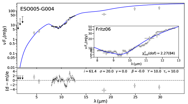
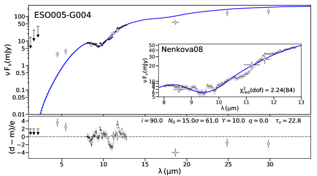
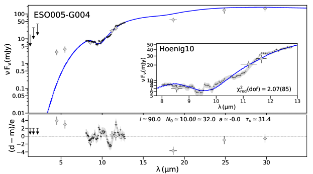
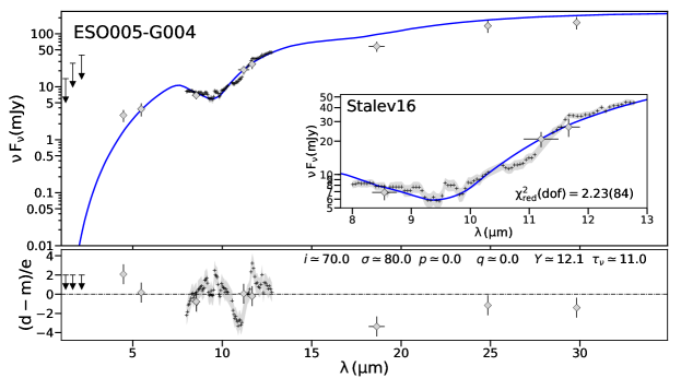
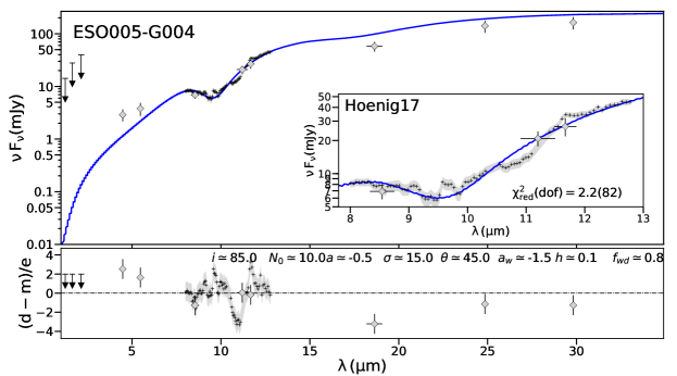
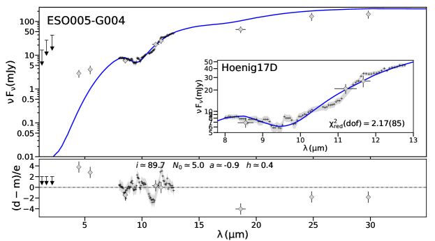
Figure 15: Nuclear IR SED of ESO005-G004. Solid blue line correspond to the best fit per torus model. Grey diamond and black crosses are the photometric data points and N-band spectrum, respectively. The black arrows represent low angular resolution data, which are treated as upper limits..

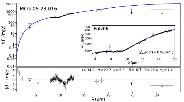
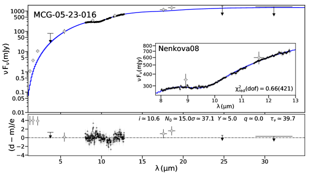
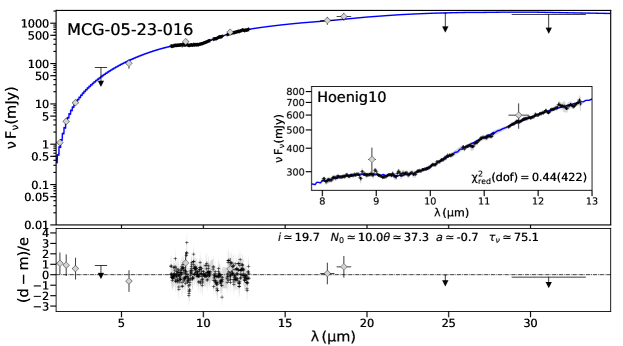
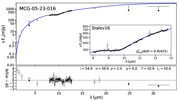
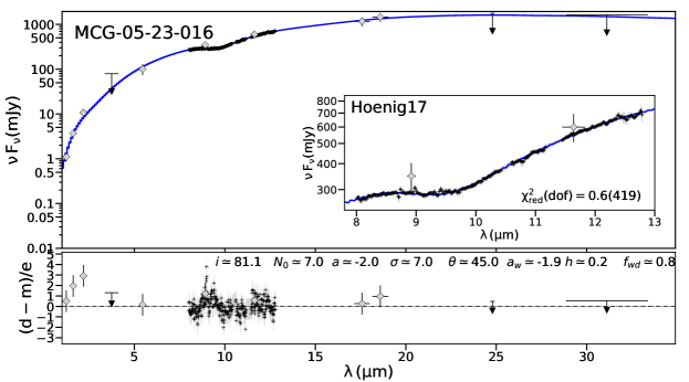
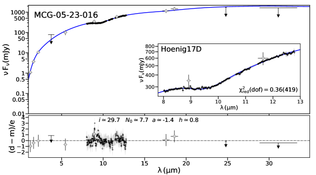
Figure 16: Same as Fig. 15 but for MCG-05-23-016.

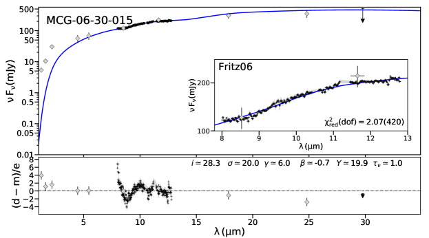
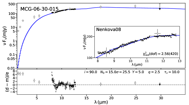
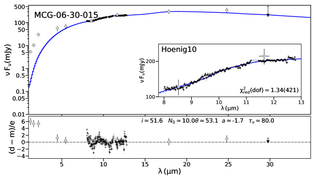
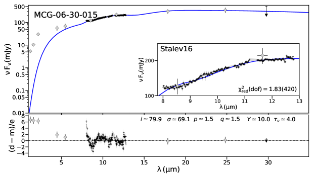
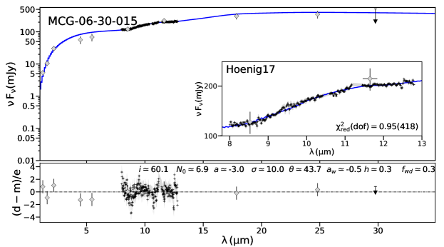
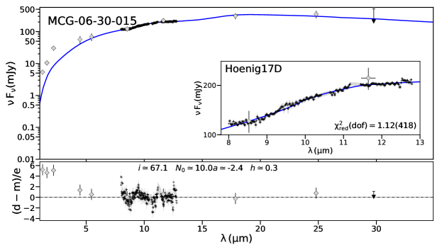
Figure 17: Same as Fig. 15 but for MCG-06-30-015.

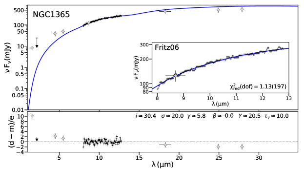
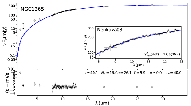
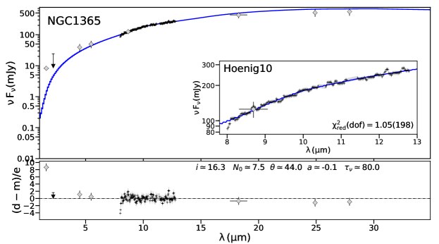
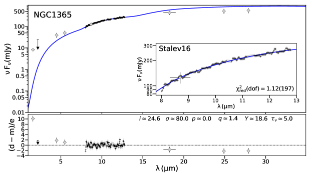
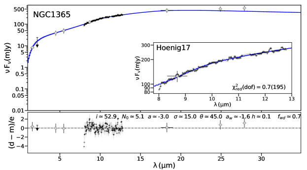
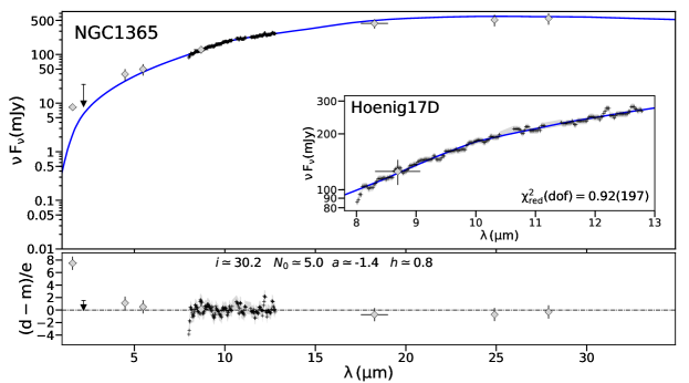
Figure 18: Same as Fig. 15 but for NGC1365.

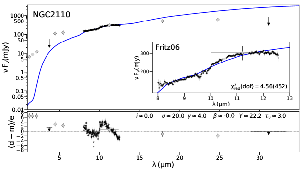
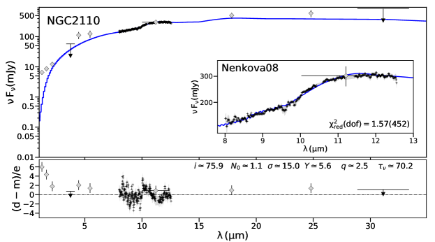
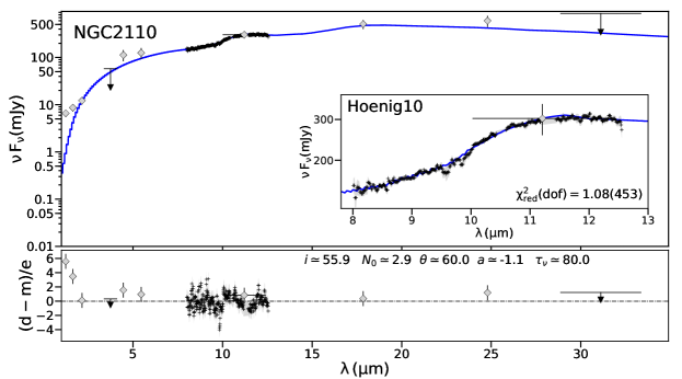
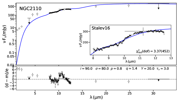
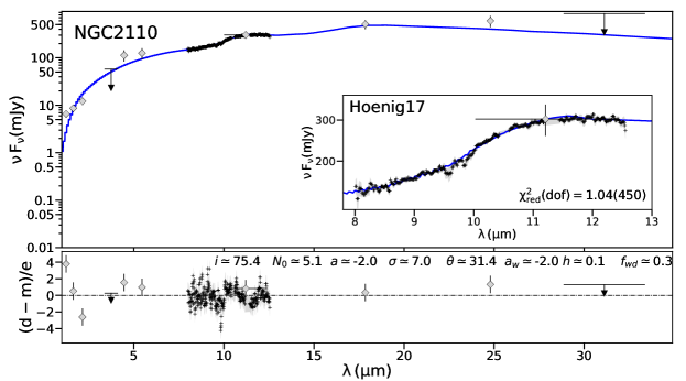
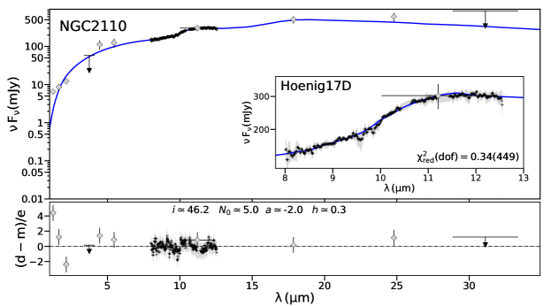
Figure 19: Same as Fig. 15 but for NGC2110.

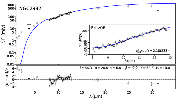
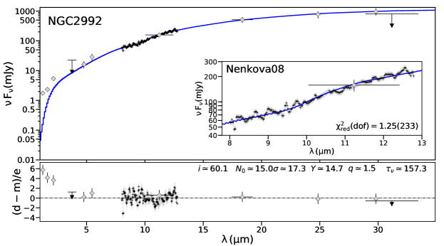
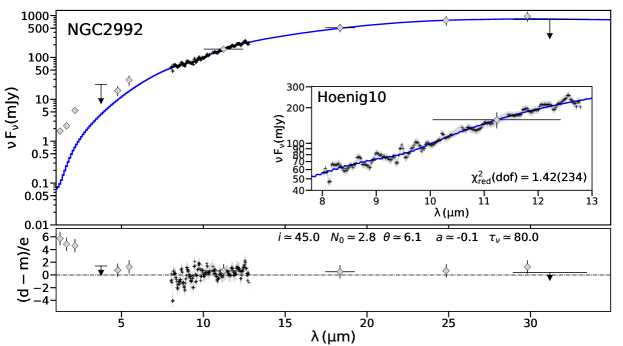
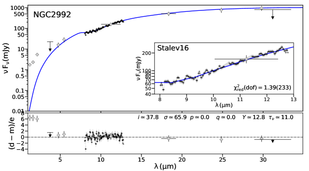
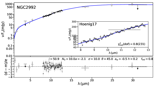
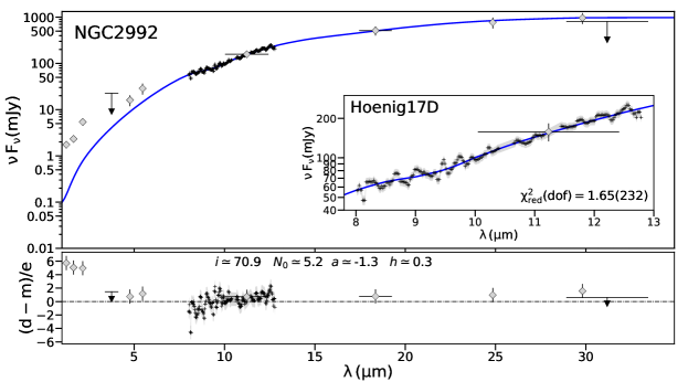
Figure 20: Same as Fig. 15 but for NGC2992.

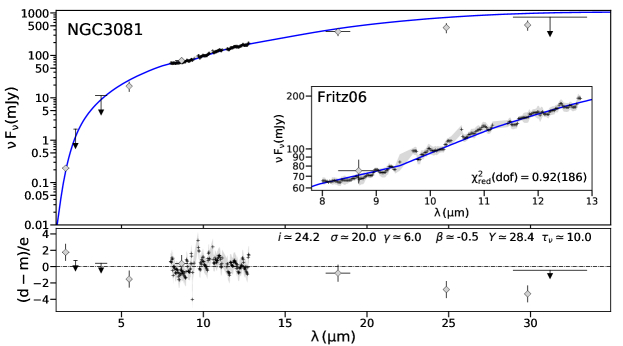
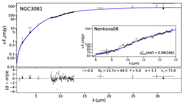
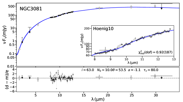
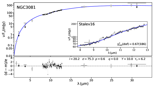
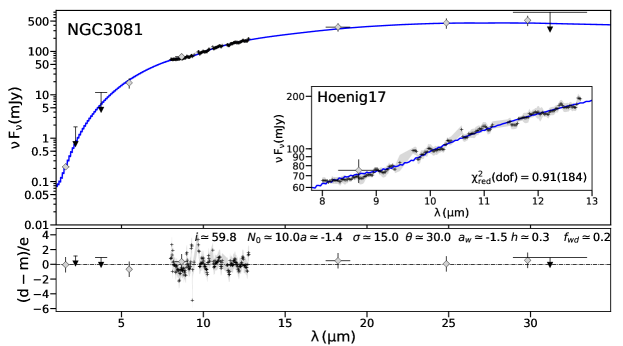
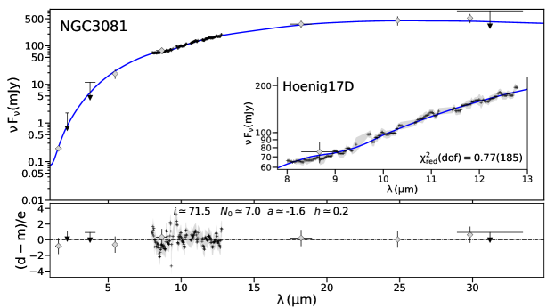
Figure 21: Same as Fig. 15 but for NGC3081.

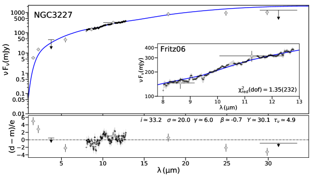
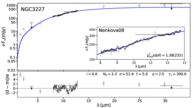
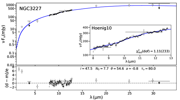
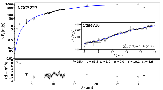
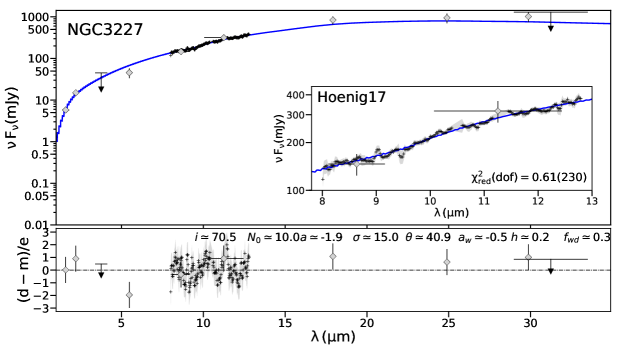
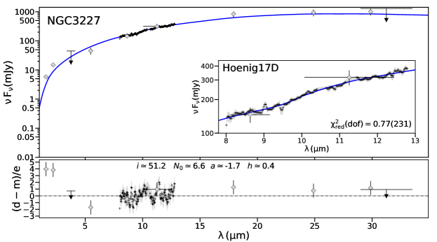
Figure 22: Same as Fig. 15 but for NGC3227.

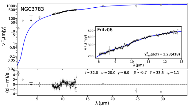
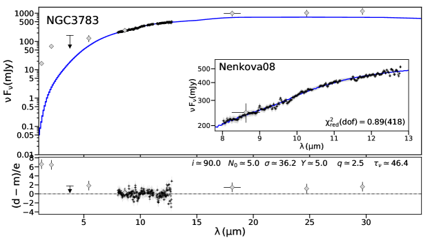
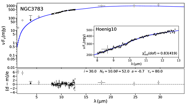
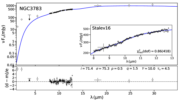
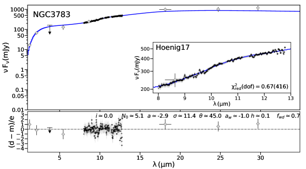
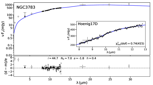
Figure 23: Same as Fig. 15 but for NGC3783.

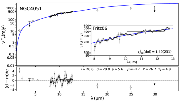
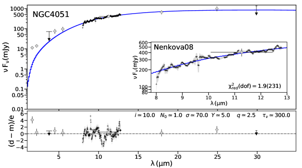
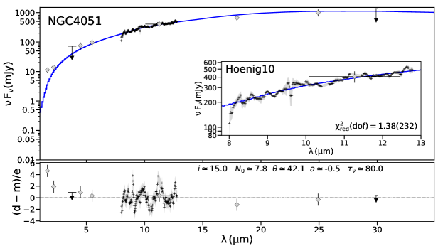
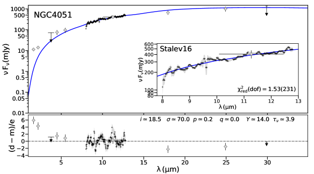
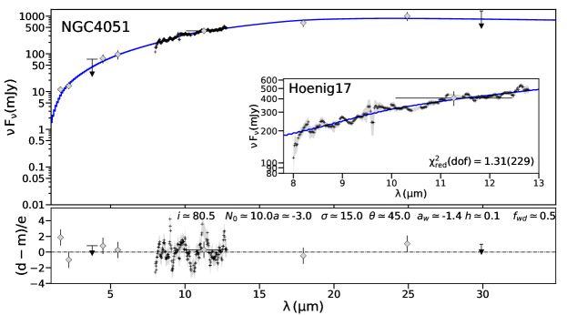
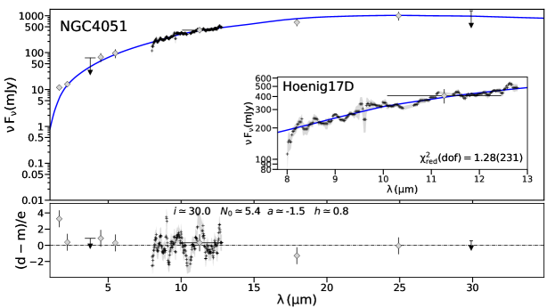
Figure 24: Same as Fig. 15 but for NGC4051.

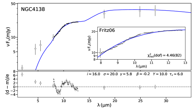
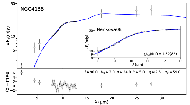
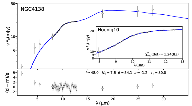
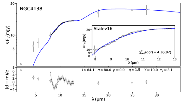
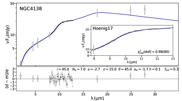
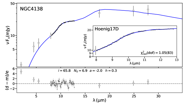
Figure 25: Same as Fig. 15 but for NGC4138.

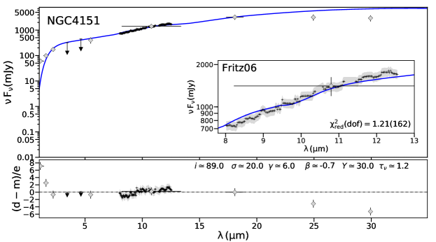
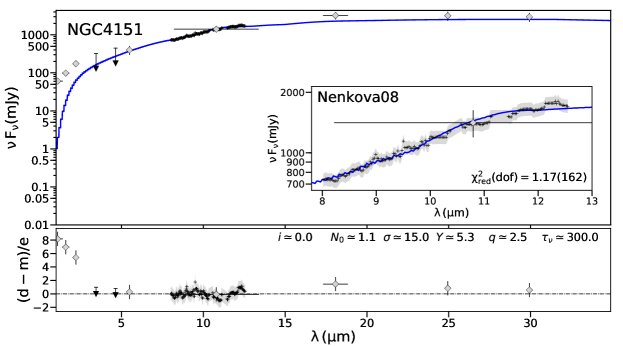
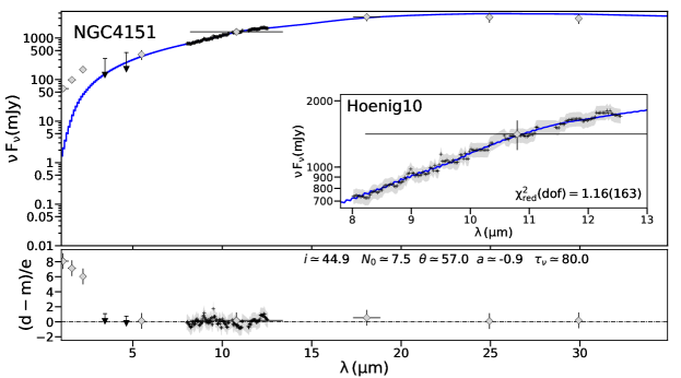
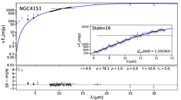
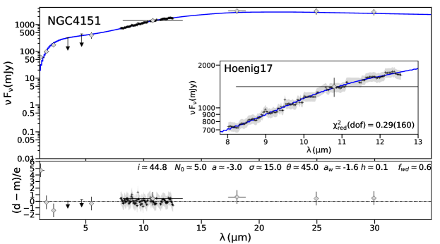
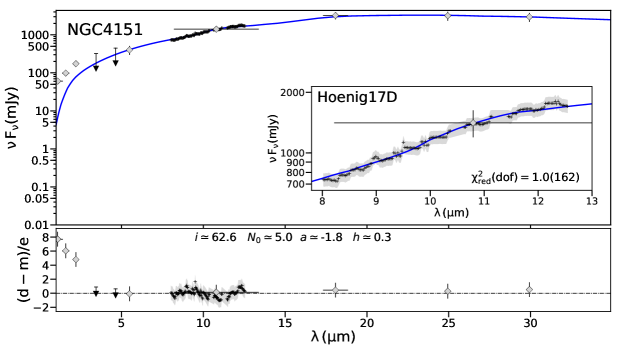
Figure 26: Same as Fig. 15 but for NGC4151.

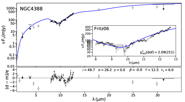
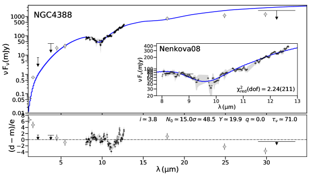
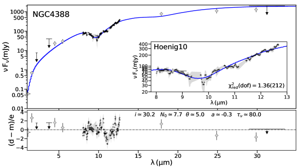
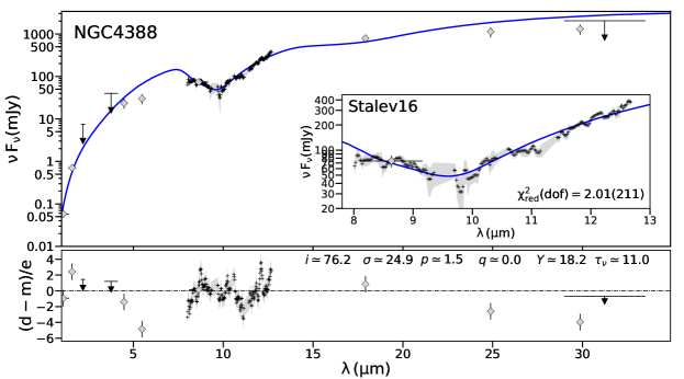
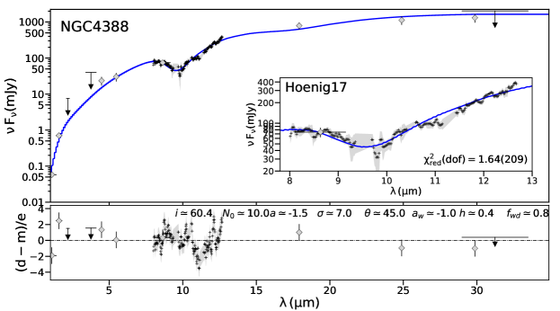
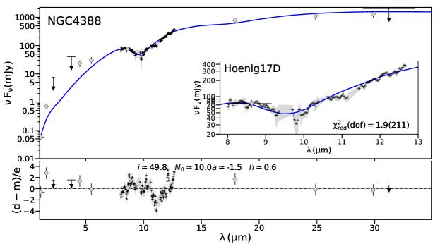
Figure 27: Same as Fig. 15 but for NGC4388.

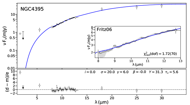
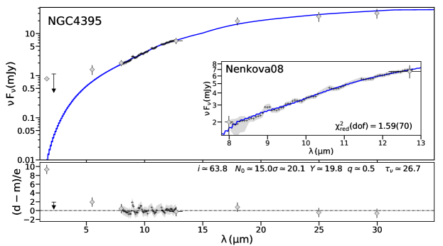
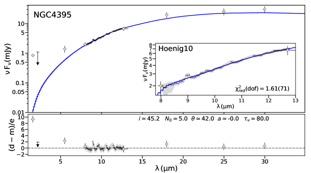
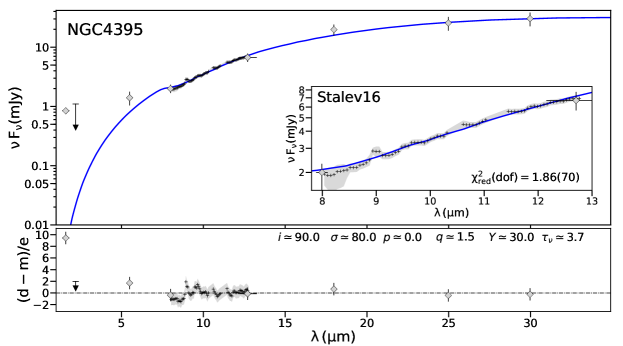
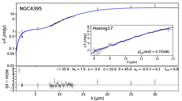
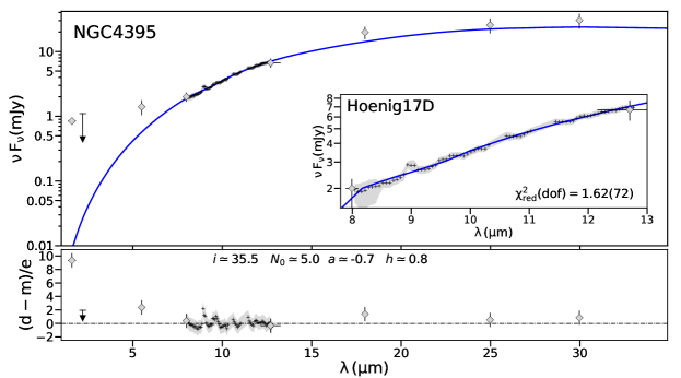
Figure 28: Same as Fig. 15 but for NGC4395.

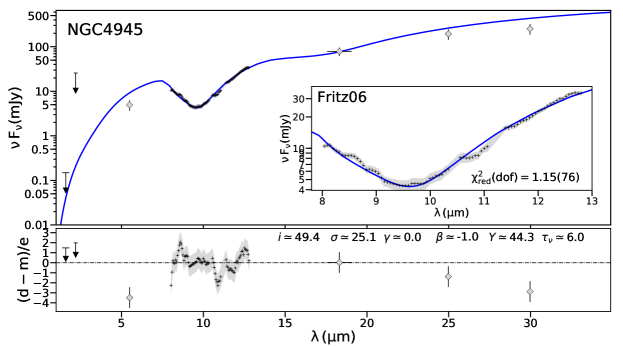
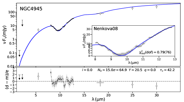
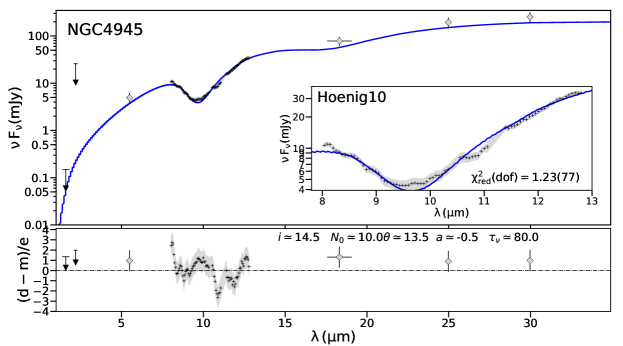
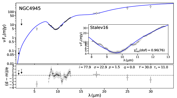
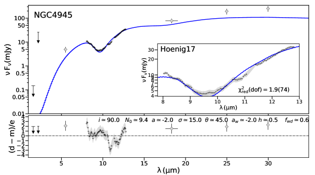
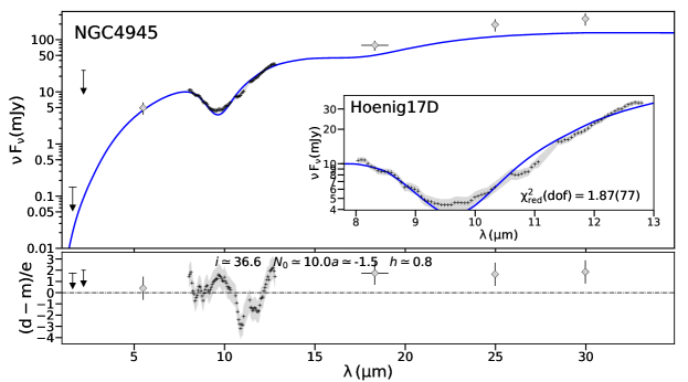
Figure 29: Same as Fig. 15 but for NGC4945.

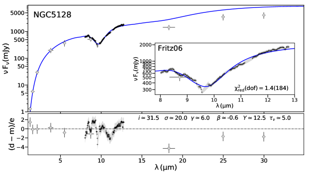
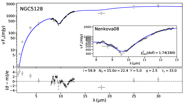
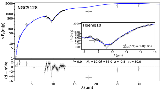
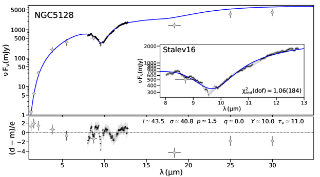
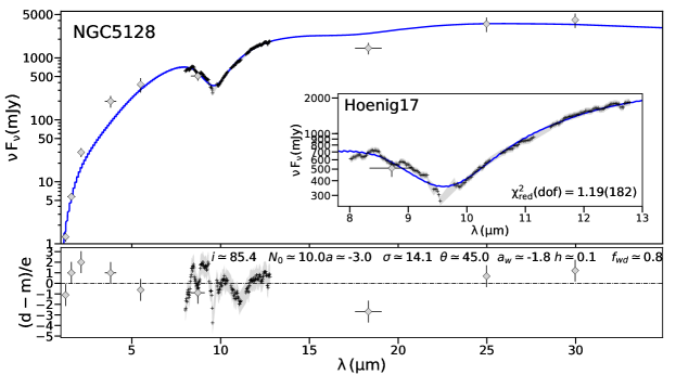
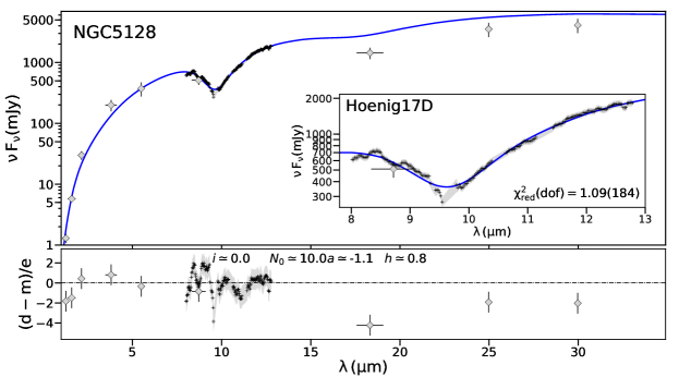
Figure 30: Same as Fig. 15 but for NGC5128.

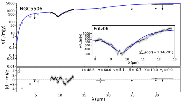
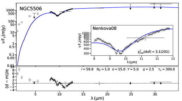
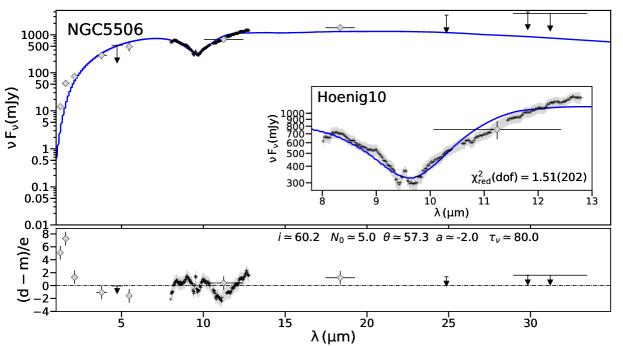
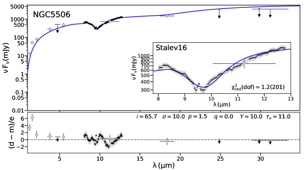
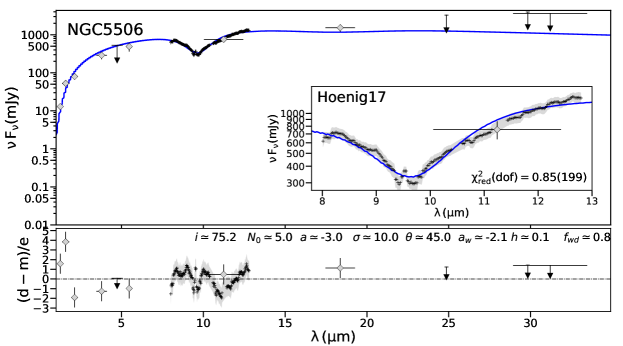
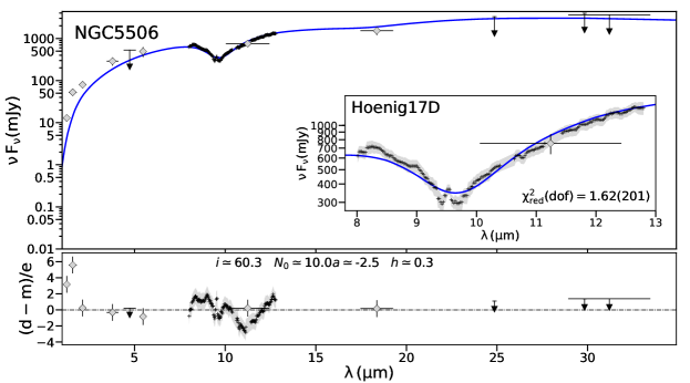
Figure 31: Same as Fig. 15 but for NGC5506.

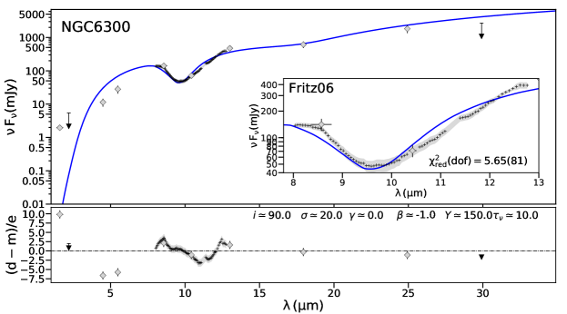
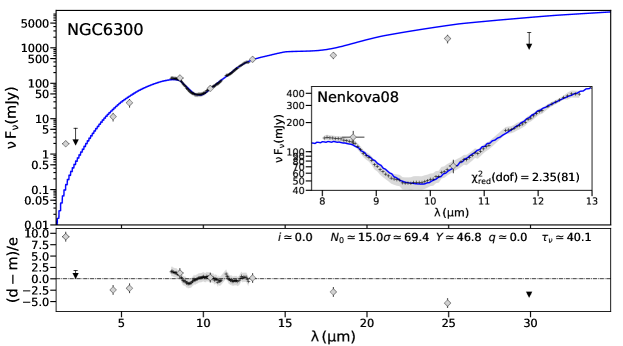
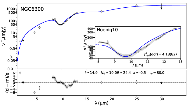
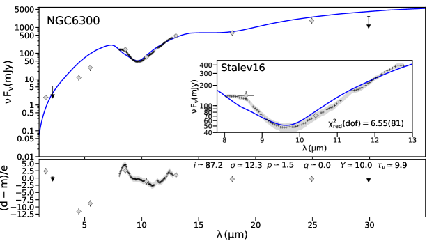
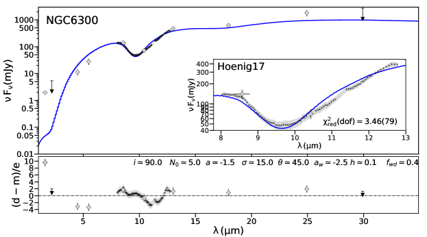
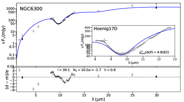
Figure 32: Same as Fig. 15 but for NGC6300.

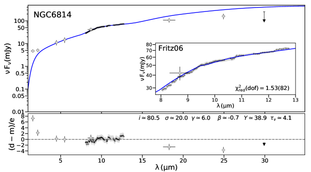
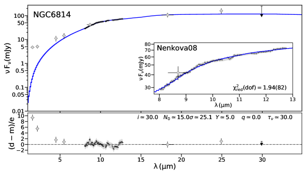
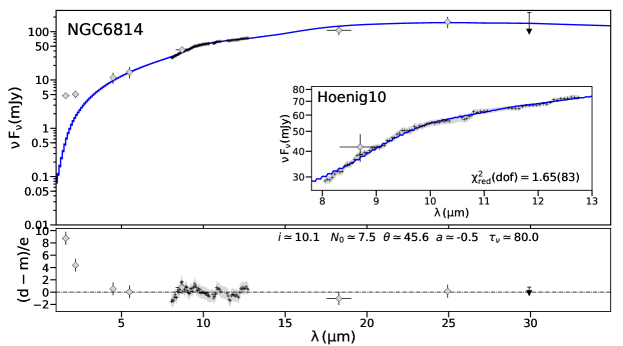
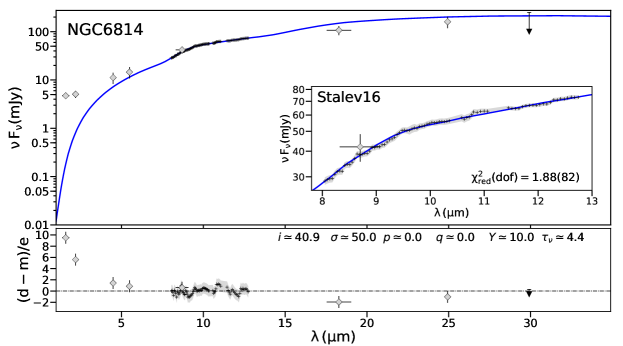
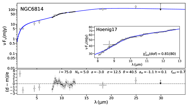
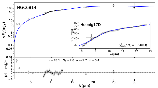
Figure 33: Same as Fig. 15 but for NGC6814.

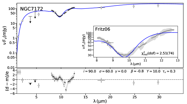
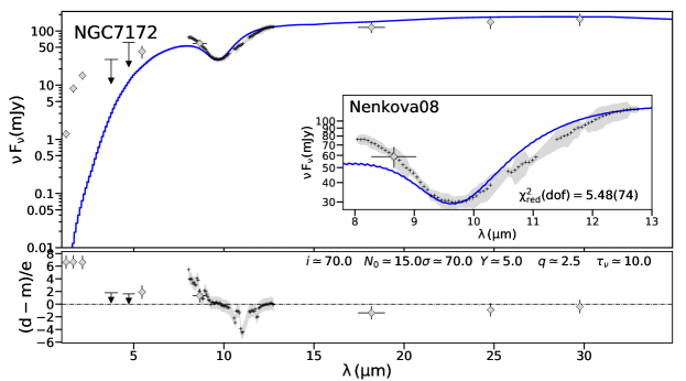
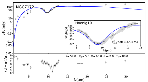
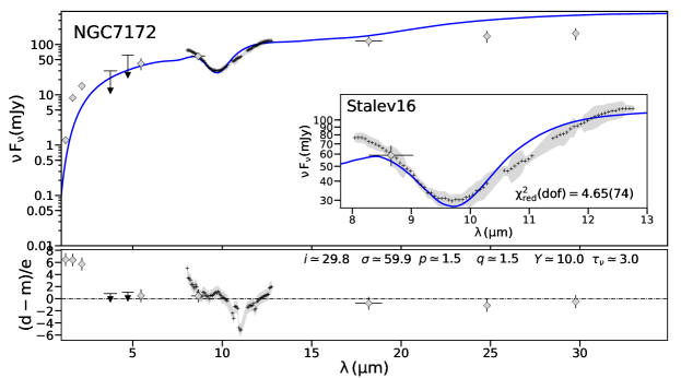
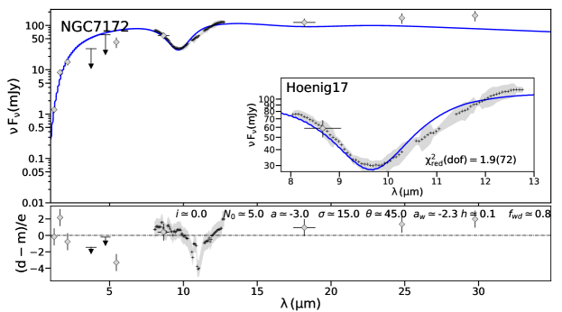
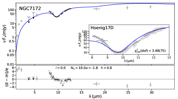
Figure 34: Same as Fig. 15 but for NGC7172.

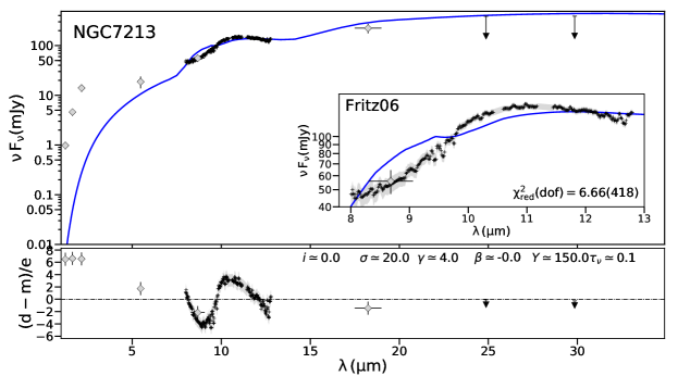
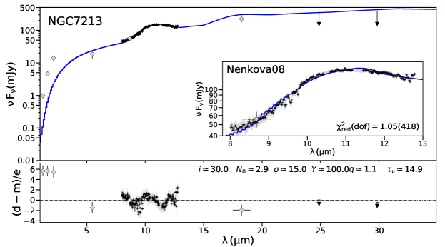
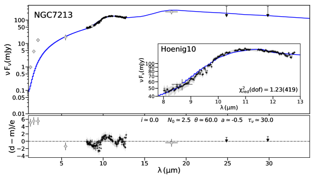
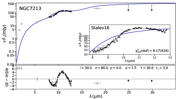
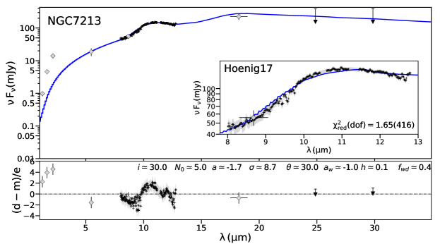
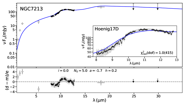
Figure 35: Same as Fig. 15 but for NGC7213.

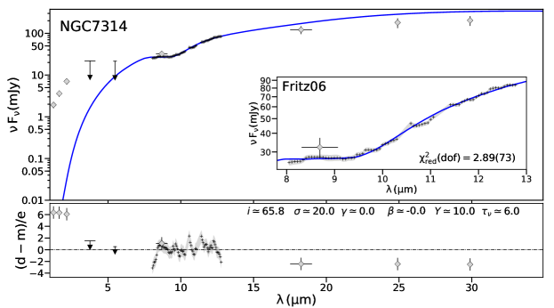
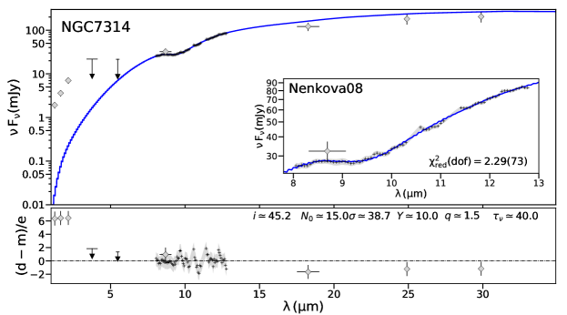
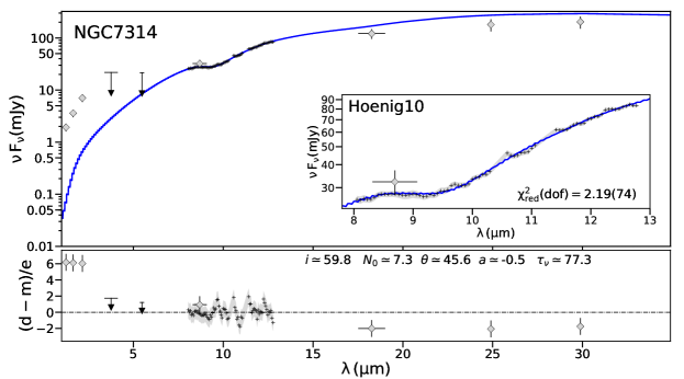
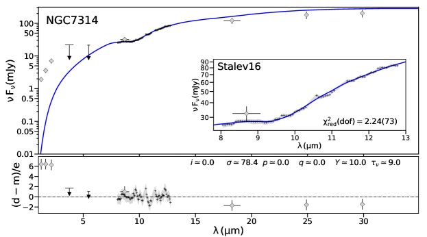
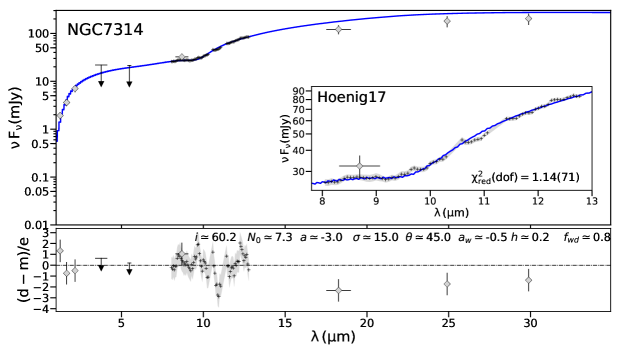
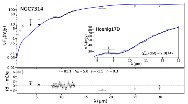
Figure 36: Same as Fig. 15 but for NGC7314.

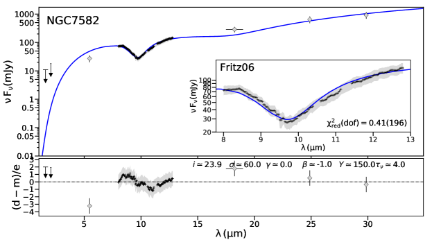
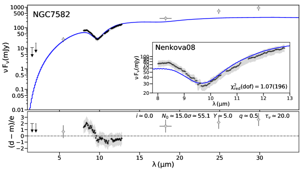
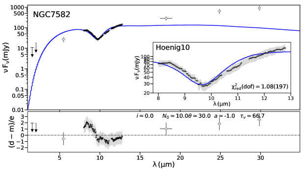
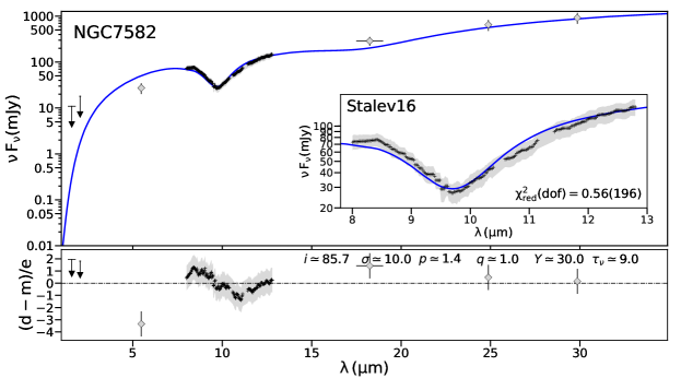
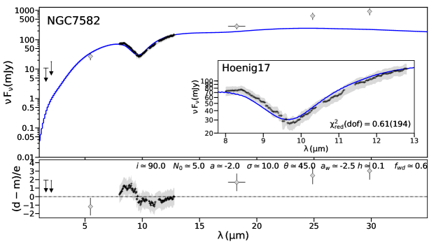
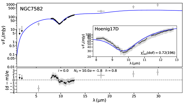
Figure 37: Same as Fig. 15 but for NGC7582.

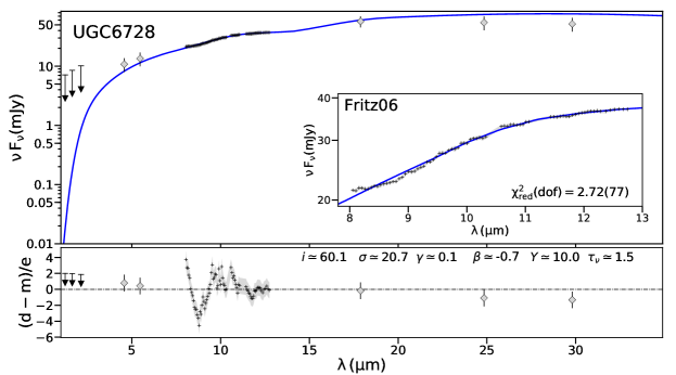
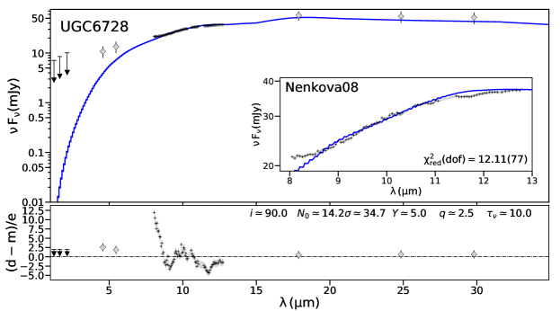
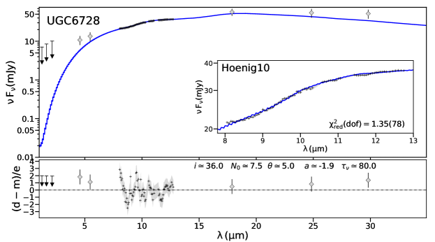
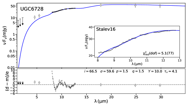
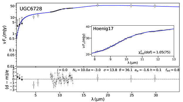
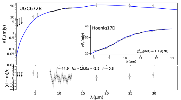
Figure 38: Same as Fig. 15 but for UGC6728.

Appendix B Combined probability distributions

In general, the various torus models provide acceptable fits ($\rm{\chi^{2}_{red}<2}$) to the majority (19/24) of the nuclear IR SEDs (see Appendix A). However, it is difficult to see trend using the individual fit parameters, which can be not well constrained. Therefore, we obtain a global statistical analysis of the torus model parameters of the various Seyfert galaxy types, rather than focusing on the individual fits. Figs. 39, 40, 41, 42 and 43 show the combined probability distribution of the different torus model parameters for all the objects in each Sy subgroup. Finally, in Tables 20, 21, 22, 23 and 24 we present the KLD results for each torus parameter and Sy subgroup.

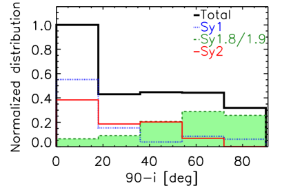
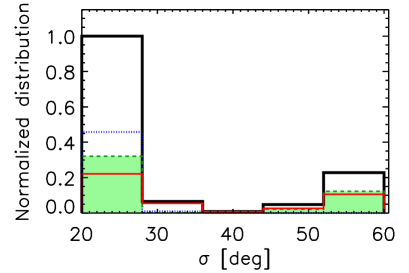
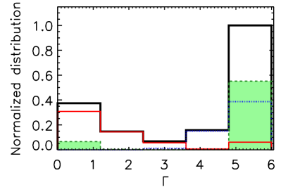
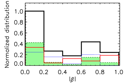
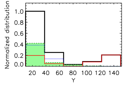
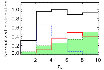
Figure 39: Comparison between the smooth F06 torus model parameter combined probability distributions. Blue dotted, green dashed, red solid and black solid lines represent the parameter distributions of Sy1, Sy1.8/1.9, Sy2 and the entire sample, respectively.

Table 12: KLD results for the smooth F06 torus models.

Subgroups	i	$\sigma$	$\Gamma$	$\beta$	Y	$\tau$	CT
(1)	(2)	(3)	(4)	(5)	(6)	(7)	(8)
Sy1s vs Sy2s	0.89	4.70	12.04	4.15	7.23	4.52	1.46
Sy1s vs Sy1.8/1.9	4.05	4.17	3.50	2.35	1.40	2.51	1.65
Sy2s vs Sy1.8/1.9	3.79	1.81	3.60	1.01	3.17	1.01	1.33

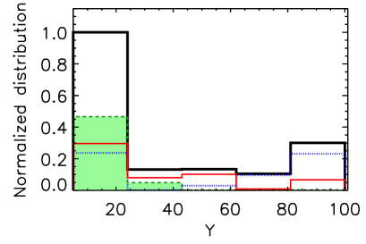
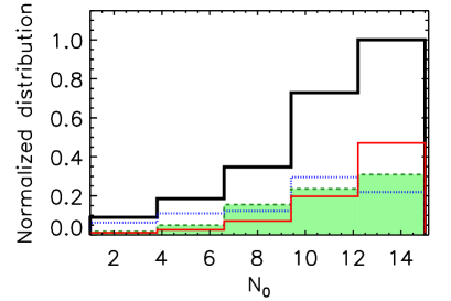
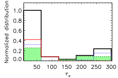
Figure 40: Same as Fig. 39 but for the clumpy NO8 torus models.

Table 13: KLD results for the clumpy N08 torus models.

Subgroups	$\sigma$	Y	N0	q	$\tau_{V}$	i	CT
(1)	(2)	(3)	(4)	(5)	(6)	(7)	(8)
Sy1s vs Sy2s	2.31	2.73	0.70	0.27	4.29	0.92	0.62
Sy1s vs Sy1.8/1.9	0.20	4.79	0.99	0.27	1.17	0.58	0.59
Sy2s vs Sy1.8/1.9	1.27	2.05	0.35	0.16	5.40	0.87	0.44

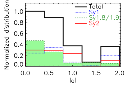
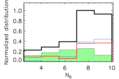
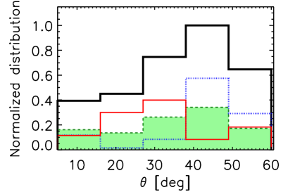
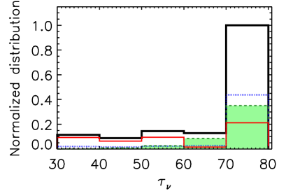
Figure 41: Same as Fig. 39 but for the clumpy H10 torus models.

Table 14: KLD results for the clumpy H10 torus models.

Subgroups	i	N0	$\theta$	a	$\tau_{V}$	CT
(1)	(2)	(3)	(4)	(5)	(6)	(7)
Sy1s vs Sy2s	1.39	1.26	2.66	1.80	1.34	0.67
Sy1s vs Sy1.8/1.9	0.81	2.24	0.69	2.57	0.31	0.48
Sy2s vs Sy1.8/1.9	0.53	0.66	0.70	1.71	1.56	0.14

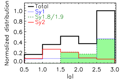
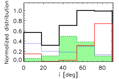
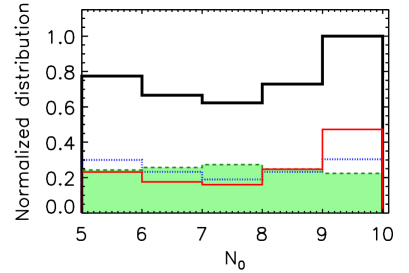
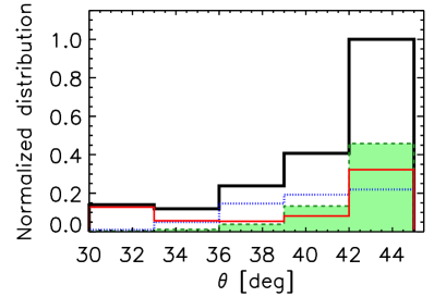
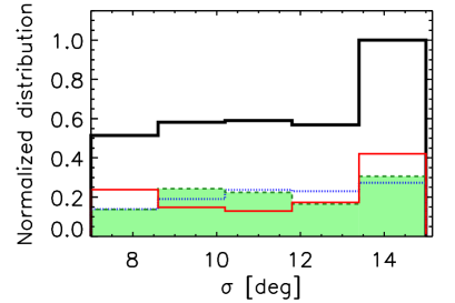
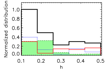
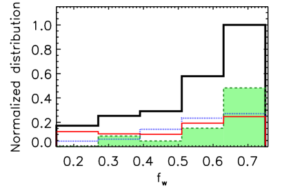
Figure 42: Same as Fig. 39 but for the clumpy disc$+$wind H17 models.

Table 15: KLD results for the clumpy disc$+$wind H17 models.

Subgroups	i	N0	a	$\theta$	$\sigma$	aw	h	fw	CT
(1)	(2)	(3)	(4)	(5)	(6)	(7)	(8)	(9)	(10)
Sy1s vs Sy2s	2.15	0.10	2.54	0.95	0.19	1.55	0.68	0.21	1.26
Sy1s vs Sy1.8/1.9	0.92	0.05	2.34	0.55	0.06	1.25	0.82	0.44	0.18
Sy2s vs Sy1.8/1.9	2.93	0.20	3.92	0.75	0.17	1.69	1.72	0.73	0.98

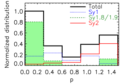
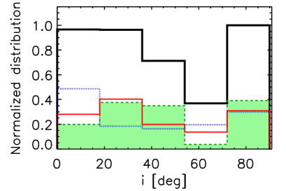
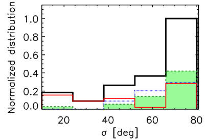
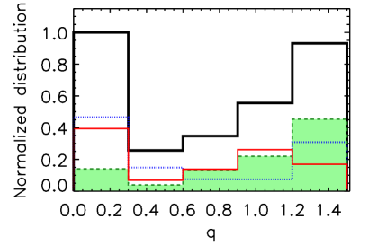
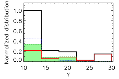
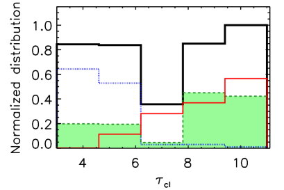
Figure 43: Same as Fig. 39 but for the two-phases S16 torus models.

Table 16: KLD results for the two-phase S16 torus models.

Subgroups	i	$\sigma$	p	q	Y	$\tau_{cl}$	CT
(1)	(2)	(3)	(4)	(5)	(6)	(7)	(8)
Sy1s vs Sy2s	0.47	4.59	3.52	0.56	2.87	5.27	0.56
Sy1s vs Sy1.8/1.9	0.89	0.96	3.51	0.88	0.42	2.18	6.99
Sy2s vs Sy1.8/1.9	0.46	5.78	6.34	0.45	1.05	1.23	4.51

Appendix C Derived torus/disc sizes and masses

For each torus model, we can derive the physical radius of the dusty torus (R_o) by using the radial extent of the torus (Y=R_o/R_d), the bolometric luminosity and the dust sublimation radius (R_d) definition (see e.g. RA11, AH11, Ichikawa et al. 2015, Esparza-Arredondo et al. 2019, GB19, GM19B, Martínez-Paredes et al. 2021). Finally, the torus gas mass for each model can be calculated as follows:

C.1 Smooth F06 torus models

The torus gas mass associated with the fitted nuclear dusty structure can be calculated as:

$${\frac{M_{torus}}{M_{\odot}}}={\frac{4\pi\leavevmode\nobreak\ m_{H}\leavevmode\nobreak\ (1.9\times 10^{21})\leavevmode\nobreak\ 1.086\leavevmode\nobreak\ (\tau_{9.7}/0.042)\leavevmode\nobreak\ R_{d}^{2}}{1.989\times 10^{30}}}$$ (2)

$$\int_{0}^{\pi/2}e^{-\gamma\left|\cos\alpha\right|}\cos\alpha\,d\alpha$$

$$\int_{1}^{Y_{0}}r^{(2-q)}\,dr$$

where the 1.9$\times 10^{21}$ value is the Galactic dust-to-gas ratio from Bohlin, Savage, & Drake (1978).

C.2 Clumpy N08 torus models

The torus gas mass associated with the fitted nuclear dusty structure can be calculated as:

$${\frac{M_{torus}}{M_{\odot}}}={\frac{4\pi\leavevmode\nobreak\ m_{H}\leavevmode\nobreak\ N_{H}^{equatorial}\leavevmode\nobreak\ R_{d}^{2}}{1.989\times 10^{30}}}\int_{0}^{\pi/2}e^{-\beta^{2}/\sigma^{2}}\cos\beta\,d\beta$$ (3)

$$\int_{1}^{Y_{0}}r^{(2-q)}\,dr$$

where $N_{H}^{equatorial}$ is:

$$N_{H}^{equatorial}=(1.9\times 10^{21})\leavevmode\nobreak\ 1.086\leavevmode\nobreak\ N_{0}\leavevmode\nobreak\ \tau_{V}\leavevmode\nobreak\ [cm^{-2}]$$ (4)

where the 1.9$\times 10^{21}$ value is the Galactic dust-to-gas ratio from Bohlin, Savage, & Drake (1978).

C.3 Clumpy H10 torus models

The torus gas mass associated with the fitted nuclear dusty structure can be calculated as (assuming b$=$1; see H10):

$${\frac{M_{torus}}{M_{\odot}}}={\frac{\pi^{1/2}\leavevmode\nobreak\ m_{H}}{R_{cl}^{2}1.989\times 10^{30}}}\leavevmode\nobreak\ \left(N_{H}^{equatorial}Erf(\theta)\right)$$

where $N_{H}^{equatorial}$ is:

$$N_{H}^{equatorial}=(1.9\times 10^{21})\leavevmode\nobreak\ 1.086\leavevmode\nobreak\ N_{0}\leavevmode\nobreak\ \tau_{V}\leavevmode\nobreak\ [cm^{-2}]$$ (5)

where the 1.9$\times 10^{21}$ value is the Galactic dust-to-gas ratio from Bohlin, Savage, & Drake (1978).

C.4 Clumpy disc$+$wind H17 models

The disc$+$wind gas mass associated with the fitted nuclear dusty structure can be calculated as (assuming b$=$1; see H10):

$${\frac{M_{torus}}{M_{\odot}}}={\frac{\pi^{1/2}\leavevmode\nobreak\ m_{H}}{R_{cl}^{2}1.989\times 10^{30}}}\leavevmode\nobreak$$

$$\left(N_{H_{w}}^{equatorial}(Erf(\theta+\sigma_{w})-Erf(\theta))+N_{H_{d}}^{equatorial}Erf(\sigma_{d})\right)$$

where $N_{H}^{equatorial}$ is:

$$N_{H}^{equatorial}=(1.9\times 10^{21})\leavevmode\nobreak\ 1.086\leavevmode\nobreak\ N_{0}\leavevmode\nobreak\ \tau_{V}\leavevmode\nobreak\ [cm^{-2}]$$ (6)

where the 1.9$\times 10^{21}$ value is the Galactic dust-to-gas ratio from Bohlin, Savage, & Drake (1978).

C.5 Two-phase S16 torus models

The torus gas mass associated with the fitted nuclear dusty structure can be calculated as:

$${\frac{M_{torus}}{M_{\odot}}}={\frac{4\pi\leavevmode\nobreak\ m_{H}\leavevmode\nobreak\ (1.9\times 10^{21})\leavevmode\nobreak\ 1.086\leavevmode\nobreak\ (\tau_{9.7}/0.042)\leavevmode\nobreak\ R_{d}^{2}}{1.989\times 10^{30}}}$$ (7)

$$\int_{0}^{\pi/2}e^{-\gamma\left|\cos\alpha\right|}\cos\alpha\,d\alpha$$

$$\int_{1}^{Y_{0}}r^{(2-q)}\,dr$$

where the 1.9$\times 10^{21}$ value is the Galactic dust-to-gas ratio from Bohlin, Savage, & Drake (1978).