The Infinity-Potential in the Square

Abstract

A representation formula for the solution of the $\infty$-Laplace equation is constructed in a punctured square, the prescribed boundary values being $u=0$ on the sides and $u=1$ at the centre. This so-called $\infty$-potential is obtained with a hodograph method. The heat equation is used and one of Jacobi’s Theta functions appears. The formula disproves a conjecture.

1 Introduction

I shall obtain a special explicit solution of the $\infty$-Laplace Equation

$$\Delta_{\infty}u:=u_{x}^{2}u_{xx}+2u_{x}u_{y}u_{xy}+u_{y}^{2}u_{yy}=0$$

in the plane. The solution is the $\infty$-potential (or the ”capacitary function”) for a square with the centre removed, at which boundary point the value $u=1$ is prescribed. On the four sides $u=0$.

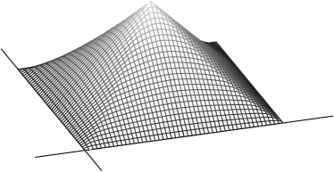
Figure 1: The graph of the solution over the square.

Let $\Omega$ be the square $0<x<2,\,0<y<2$. I shall show that the viscosity solution of the Dirichlet problem just described is

$$u(x,y)=\min_{\theta\in[0,\pi/2]}\max_{r\in[0,1]}\Big{\{}r(x\cos\theta+y\sin\theta)-W(r,\theta)\Big{\}}$$ (1.1)

where

$$W(r,\theta) =\frac{8}{\pi}\left(\frac{r^{4}}{6}\sin(2\theta)+\frac{r^{36}}{210}\sin(6\theta)+\frac{r^{100}}{990}\sin(10\theta)+\cdots\right).$$

The formula is valid in the quadrant $0\leq x\leq 1$, $0\leq y\leq 1$, and the obvious symmetries extends the solution to the whole $\overline{\Omega}$. So far as we know, the only hitherto known explicit $\infty$-potentials are for stadium-like domains with solutions on the form $\operatorname{dist}(\mathbf{x},\partial\Omega)$.

The explicit solution (1.1) settles a conjecture, indicated in [JLM99] and [JLM01]. A calculation shows that $u$ is not a solution to the $\infty$-eigenvalue problem

$$\max\left\{\Lambda-\frac{|\nabla u|}{u},\;\Delta_{\infty}u\right\}=0,\qquad u|_{\partial\Omega}=0.$$

Se also [Yu07].

The $\infty$-Laplace equation $\Delta_{\infty}u=0$ was introduced by G. Aronsson in 1967 as the limit of the $p$-Laplace equation

$$\Delta_{p}u:=\operatorname{div}\left(|\nabla u|^{p-2}\nabla u\right)=0$$

when $p\to\infty$. See [Aro67], [Aro68]. For this 2 order equation, the concept of viscosity solutions was introduced by T. Bhattacharya, E. DiBenedetto, and J. Manfredi in [BDM89], and uniqueness of such solutions with continuous boundary values was proved by R. Jensen, cf. [Jen93]. For the $p$-Laplace equation, the capacitary problem in convex rings was studied by J. Lewis, [Lew77]. A detailed investigation of this problem for the $\infty$-Laplace equation was given in [LL19], [LL21].

I use the hodograph method, according to which a linear equation is produced for a function $w=w(p,q)$ in the new coordinates

$$p=\frac{\partial u(x,y)}{\partial x},\qquad q=\frac{\partial u(x,y)}{\partial y}.$$

A solution $W(r,\theta)=w(r\cos\theta,r\sin\theta)$ is constructed with judiciously adjusted boundary values. When transforming back we get a formula for $u$ in terms of its gradient, which, in turn, is shown to be a critical value of the objective function in (1.1). The critical point – that is, the obtained minimax $(r,\theta)$ – is the length $r=|\nabla u|$ and the direction $\theta=\arg\nabla u$ of the gradient at $(x,y)$. A full account is given in Section 6.

It is interesting that the 2 Jacobi Theta function

$$\vartheta_{2}(z,q)=2\sum_{k=1}^{\infty}q^{(k-1/2)^{2}}\cos((2k-1)z)$$

appears in the formulas. For example, we shall see that

$$u=\frac{4}{\pi}\int_{0}^{\arg\nabla u}\vartheta_{2}\left(2\psi,|\nabla u|^{16}\right)\mathrm{\,d}\psi,\qquad 0\leq\arg\nabla u\leq\pi/2,$$

and that the determinant of the Hessian matrix of $u$ is

$$\det\mathcal{H}u=-\frac{\pi^{2}}{16}|\nabla u|^{4}\,\vartheta_{2}^{-2}\left(2\arg\nabla u,|\nabla u|^{16}\right),\qquad\arg\nabla u\neq(2k-1)\pi/4.$$

An immediate consequence of the last identity is that $u$ is not $C^{2}$ on the diagonals of the square. Indeed, the symmetries yield $\arg\nabla u(x,x)=\pi/4$ and $\vartheta_{2}$ is zero for odd integer multiples of $z=\pi/2$.

Write

$$D_{1}:=\{(r,\theta)\;|\;0<r<1,\,0<\theta<\pi/2\}.$$

Define $W\colon\overline{D}_{1}\to\mathbb{R}$, as

$$W(r,\theta):=\frac{8}{\pi}\sum_{n=1}^{\infty}\frac{r^{m_{n}^{2}}}{\left(m_{n}^{2}-1\right)m_{n}}\sin\left(m_{n}\theta\right),\qquad m_{n}=4n-2,$$ (1.2)

and let $u\colon\overline{\Omega}\to\mathbb{R}$ be the extension of formula (1.1) to $\overline{\Omega}$. I prove

Theorem 1.1.

The function $u$ is the unique viscosity solution of the problem

$$\begin{cases}\Delta_{\infty}u=0\qquad&\text{in $\Omega\setminus\{(1,1)\}$},\\ u=0&\text{on $\partial\Omega$,}\\ u=1&\text{at $(1,1)$,}\end{cases}$$ (1.3)

in the square $\Omega=\{(x,y)\;|\;0<x<2,\,0<y<2\}$. Moreover, $u\in C^{1}(\overline{\Omega}\setminus\{(1,1)\})$ and $u$ is real-analytic, except at the diagonals and medians.

Actually, we do not know how smooth $u$ is across the medians.

2 Proof of the Theorem

The coefficients in $W$ and the exponents on $r$ are chosen so that $W(1,\theta)$ is the Fourier series for the odd $\pi$-periodic extension of $\cos\theta+\sin\theta-1$, and so that $rW_{r}+W_{\theta\theta}=0$. Thus, $W$ is the solution of the problem

$$\begin{cases}rW_{r}+W_{\theta\theta}=0\qquad&\text{in $D_{1}$},\\ W(r,0)=W(r,\pi/2)=0,&0\leq r\leq 1,\\ W(0,\theta)=0,\\ W(1,\theta)=\cos\theta+\sin\theta-1,&0\leq\theta\leq\pi/2.\end{cases}$$ (2.1)

I prove first that (1.1) is the viscosity solution to the Dirichlet problem

$$\begin{cases}\Delta_{\infty}u=0\qquad&\text{in $\Omega_{1}$},\\ u(0,t)=u(t,0)=0,&\\ u(1,t)=u(t,1)=t&\text{for $0\leq t\leq 1$,}\end{cases}$$ (2.2)

where

$$\Omega_{1}:=\{(x,y)\;|\;0<x<1,\,0<y<1\}.$$

We know in advance that the solution must be linear on the medians. It is then straight forward to show that the gluing (2.15) of the translations and rotations of (1.1) is the solution of the original problem (1.3).

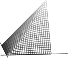
Figure 2: The solution to problem (2.2) over the square $\overline{\Omega}_{1}=[0,1]^{2}$.

For each $(x,y)\in\overline{\Omega}_{1}$ I denote the objective function $f_{(x,y)}\colon\overline{D}_{1}\to\mathbb{R}$ in (1.1) by

$$f_{(x,y)}(r,\theta):=r(x\cos\theta+y\sin\theta)-W(r,\theta).$$

Note that we immediately have

$$u(x,y)\geq\min_{\theta\in[0,\pi/2]}f_{(x,y)}(0,\theta)=0.$$

The bounds in the Proposition below show that the correct boundary values are obtained.

Proposition 2.1.

For all $(x,y)\in\overline{\Omega}_{1}$,

$$1-\sqrt{(1-x)^{2}+(1-y)^{2}}\leq u(x,y)\leq\operatorname{dist}((x,y),\partial\Omega).$$

Proof.

$$u(x,y) =\min_{\theta\in[0,\pi/2]}\max_{r\in[0,1]}f_{(x,y)}(r,\theta)$$

$$\geq\min_{\theta\in[0,\pi/2]}f_{(x,y)}(1,\theta)$$

$$=\min_{\theta\in[0,\pi/2]}\left\{x\cos\theta+y\sin\theta-(\cos\theta+\sin\theta-1)\right\}$$

$$=1-\max_{\theta\in[0,\pi/2]}\left\{(1-x)\cos\theta+(1-y)\sin\theta\right\}$$

$$=1-\sqrt{(1-x)^{2}+(1-y)^{2}}\max_{\theta\in[0,\pi/2]}\cos\left(\theta-\phi\right)$$

where the last line is due to a standard trigonometric identity. The lower bound is confirmed, since the maximum is at $\theta=\phi:=\arctan\frac{1-y}{1-x}\in[0,\pi/2]$.

Since $W\geq 0$ (see Lemma 2.1),

$$u(x,y) =\min_{\theta\in[0,\pi/2]}\max_{r\in[0,1]}f_{(x,y)}(r,\theta)$$

$$\leq\min_{\theta\in[0,\pi/2]}\max_{r\in[0,1]}\left\{r(x\cos\theta+y\sin\theta)\right\}$$

$$=\min_{\theta\in[0,\pi/2]}\left\{x\cos\theta+y\sin\theta\right\}$$

$$=\min\left\{x,y\right\}=\operatorname{dist}((x,y),\partial\Omega).$$

∎

I prove next that $u$ is $\infty$-harmonic in the viscosity sense in $\Omega_{1}$. The strategy is to first show that $u$ is a classical solution in $\Omega_{1}$ except on the diagonal. At the diagonal it is necessary to demonstrate that the smoothness breaks down in such a way that no test function can touch $u$ from below. Yet, it is essential to know that $u$ is $C^{1}$, because we need the gradient of a test function to align with the diagonal when the touching is from above. The proof is then completed by showing that $x\mapsto u(x,x)$ is convex.

It turns out that the Heat Equation is helpful. Consider an insulated rod of length $\pi/2$ with initial temperature $v(0,\theta)=1$, for $0<\theta<\pi/2$. Suppose the rod is subjected to the heat equation $v_{t}=v_{\theta\theta}$ with boundary conditions $v(t,0)=v(t,\pi/2)=0$ when $t>0$. The solution of this textbook example is

$$v(t,\theta)=\frac{8}{\pi}\sum_{n=1}^{\infty}\frac{e^{-m_{n}^{2}t}}{m_{n}}\sin(m_{n}\theta),\qquad m_{n}=4n-2.$$

It becomes

$$U(r,\theta):=rW_{r}(r,\theta)-W(r,\theta)=\frac{8}{\pi}\sum_{n=1}^{\infty}\frac{r^{m_{n}^{2}}}{m_{n}}\sin(m_{n}\theta)$$ (2.3)

under the substitution

$$r=e^{-t}.$$

Since $W\in C(\overline{D}_{1})$ with $W(1,0)=W(1,\pi/2)=0$, an immediate consequence is that $W_{r}(r,\theta)$ has jumps from 0 to 1 at the two corner points $r=1$, $\theta=0$ and $r=1$, $\theta=\pi/2$. Otherwise it is continuous up to the boundary $\partial D_{1}$.

The temperature $v(t,\theta)$ is strictly decreasing. To see this note that $h:=v_{t}$ is again caloric with initial values $h(0,\theta)\leq 0$ and lateral values $h(t,0)=h(t,\pi/2)=0$. The strong maximum principle then yields $h<0$ at inner points, since certainly $h\not\equiv 0$. Since $U_{r}=rW_{rr}$ it follows that

$$0>v_{t}=U_{r}\frac{\mathrm{\,d}r}{\mathrm{\,d}t}=-r^{2}W_{rr}$$

and $W_{rr}>0$ in $D_{1}$. Integrating back, we see that also $W_{r}$ and $W$ are positive in $D_{1}$. Moreover, $U_{\theta\theta}=v_{\theta\theta}=v_{t}<0$ and

$$\theta\mapsto U_{\theta}(r,\theta)=rW_{r\theta}(r,\theta)-W_{\theta}(r,\theta)=\frac{8}{\pi}\sum_{n=1}^{\infty}r^{m_{n}^{2}}\cos(m_{n}\theta)$$

is therefore strictly decreasing for each $0<r<1$. Its zero is obviously at $\theta=\pi/4$. The following Lemma is proved.

Lemma 2.1.

Let $W\colon\overline{D}_{1}\to\mathbb{R}$ be the series defined in (1.2).

1. The functions $W$, $W_{r}$, and $W_{rr}$ are positive in $D_{1}$.

2. $W,W_{\theta}\in C\left(\overline{D}_{1}\right)$, and $W_{r}\in C\left(\overline{D}_{1}\setminus\{(1,0),(1,\pi/2)\}\right)$. $W_{r}$ is discontinuous at the two points $(r,\theta)=(1,0)$ and $(r,\theta)=(1,\pi/2)$.

3. For $0<r<1$,

   $$U_{\theta}(r,\theta)=rW_{r\theta}(r,\theta)-W_{\theta}(r,\theta)$$

   is positive when $0\leq\theta<\pi/4$, negative when $\pi/4<\theta\leq\pi/2$, and thus zero in $D_{1}$ precisely when $\theta=\pi/4$.

Let

$$B_{1}:=\left\{(p,q)\,|\,0<p^{2}+q^{2}<1,\;p>0,\,q>0\right\}$$

be the sector in the first quadrant and define $w\colon\overline{B}_{1}\to\mathbb{R}$ as $W$ in Cartesian coordinates, i.e., $w(r\cos\theta,r\sin\theta):=W(r,\theta)$. I shift to vector notation

$$\mathbf{x}:=[x,y]^{\top}\in\overline{\Omega}_{1},\,\mathbf{p}:=[p,q]^{\top}\in\overline{B}_{1},\,\mathbf{r}:=[r,\theta]^{\top}\in\overline{D}_{1},$$

and denote by $\Phi$ the coordinate transformation $\Phi\colon\overline{D}_{1}\to\overline{B}_{1}$. i.e.,

$$\Phi(\mathbf{r})=\Phi(r,\theta):=\begin{bmatrix}r\cos\theta\\ r\sin\theta\end{bmatrix}=\begin{bmatrix}p\\ q\end{bmatrix}=\mathbf{p}.$$

Now,

$$W(\mathbf{r})=w(\Phi(\mathbf{r}))$$

and $\nabla W(\mathbf{r})=\nabla w(\Phi(\mathbf{r}))\nabla\Phi(\mathbf{r})$ where $\nabla W=[W_{r},W_{\theta}]$, $\nabla w=[w_{p},w_{q}]$, and

$$\nabla\Phi=\begin{bmatrix}\nabla(r\cos\theta)\\ \nabla(r\sin\theta)\end{bmatrix}=\begin{bmatrix}\cos\theta&-r\sin\theta\\ \sin\theta&r\cos\theta\end{bmatrix}$$

is the Jacobian matrix of $\Phi$.

In the next Lemma, I establish that for every $\mathbf{x}=[x,y]^{\top}\in\Omega_{1}$ the minimax in (1.1) is obtained at a unique point $\mathbf{r}=[r,\theta]^{\top}\in D_{1}$. The result is crucial because it allows us to set up a correspondence $\mathbf{g}\colon\Omega_{1}\to B_{1}$ as

$$\mathbf{g}(\mathbf{x})=\mathbf{g}(x,y):=\begin{bmatrix}r\cos\theta\\ r\sin\theta\end{bmatrix}=\Phi(\mathbf{r}),\qquad\text{$[r,\theta]^{\top}\in D_{1}$ is \emph{the} minimax in \eqref{eq:solution}.}$$ (2.4)

Lemma 2.2.

Fix $[x,y]^{\top}\in\Omega_{1}$. The gradient of the objective function

$$\begin{bmatrix}r\\ \theta\end{bmatrix}\mapsto f_{\mathbf{x}}(r,\theta)=r(x\cos\theta+y\sin\theta)-W(r,\theta)$$

is zero at exactly one point in $\overline{D}_{1}$. This critical point is an interior minimax.

Of course, the critical value is $u(x,y)$ as defined in (1.1).

Proof.

Let $\mathbf{x}=[x,y]^{\top}\in\Omega_{1}$ and assume first that $\theta\in(0,\pi/2)$. Then the partial derivative of the objective function

$$r\mapsto\frac{\partial}{\partial r}f_{\mathbf{x}}(r,\theta)=x\cos\theta+y\sin\theta-W_{r}(r,\theta)$$

is continuous up to the boundary (Lemma 2.1 (II)) with end-point values

$$\frac{\partial}{\partial r}f_{\mathbf{x}}(0,\theta)=x\cos\theta+y\sin\theta-0>0$$

and

$$\frac{\partial}{\partial r}f_{\mathbf{x}}(1,\theta) =x\cos\theta+y\sin\theta-W_{r}(1,\theta)$$

$$=x\cos\theta+y\sin\theta+W_{\theta\theta}(1,\theta)$$

$$=x\cos\theta+y\sin\theta-\cos\theta-\sin\theta$$

$$=-(1-x)\cos\theta-(1-y)\sin\theta<0.$$

Thus, $f_{\mathbf{x}}(\cdot,\theta)$ has an interior maximum for each fixed $\theta\in(0,\pi/2)$. It is unique since

$$\frac{\partial^{2}}{\partial r^{2}}f_{\mathbf{x}}(r,\theta)=-W_{rr}(r,\theta)<0$$

by Lemma 2.1 (I). It occurs at $r$ where

$$0=\frac{\partial}{\partial r}f_{\mathbf{x}}(r,\theta)=x\cos\theta+y\sin\theta-W_{r}(r,\theta)$$

and by the implicit function theorem there is an analytic function $r_{\mathbf{x}}\colon(0,\pi/2)\to(0,1)$ so that

$$W_{r}(r_{\mathbf{x}}(\theta),\theta)=x\cos\theta+y\sin\theta.$$ (2.5)

At $\theta=0$ and $\theta=\pi/2$ we have $f_{\mathbf{x}}(r,0)=rx$ and $f_{\mathbf{x}}(r,\pi/2)=ry$ with maximum value $x$ and $y$, respectively, at $r=1$. We thus extend the function $r_{\mathbf{x}}$ to the closed interval $[0,\pi/2]$ by defining $r_{\mathbf{x}}(0)=r_{\mathbf{x}}(\pi/2)=1$.

Observe that the limit

$$\lim_{\theta\to 0^{+}}W_{r}(r_{\mathbf{x}}(\theta),\theta)=\lim_{\theta\to 0^{+}}(x\cos\theta+y\sin\theta)=x>0$$

exists. Since $W_{r}(r,0)=0$ for all $0\leq r\leq 1$, the only possibility is that $r_{\mathbf{x}}(\theta)\to 1$. Recall that $W_{r}$ is not continuous at $r=1$, $\theta=0$ (Lemma 2.1 (II)). Similarly, $r_{\mathbf{x}}(\theta)\to 1$ also when $\theta\to\pi/2^{-}$ and we conclude that $r_{\mathbf{x}}$ is continuous up to the boundary.

We can now write

$$h_{\mathbf{x}}(\theta):=\max_{r\in[0,1]}f_{\mathbf{x}}(r,\theta)=r_{\mathbf{x}}(\theta)(x\cos\theta+y\sin\theta)-W(r_{\mathbf{x}}(\theta),\theta),\quad\theta\in[0,\pi/2],$$

and any critical point of $f_{\mathbf{x}}$ must occur at $[r_{\mathbf{x}}(\theta),\theta]^{\top}$ for some $\theta\in[0,\pi/2]$.

Note again that $h_{\mathbf{x}}$ is continuous and analytic in the interior. Differentiating yields

$$h_{\mathbf{x}}^{\prime}(\theta) =r_{\mathbf{x}}^{\prime}(\theta)(x\cos\theta+y\sin\theta)+r_{\mathbf{x}}(\theta)(-x\sin\theta+y\cos\theta)$$

$$\quad{}-r_{\mathbf{x}}^{\prime}(\theta)W_{r}(r_{\mathbf{x}}(\theta),\theta)-W_{\theta}(r_{\mathbf{x}}(\theta),\theta)$$

$$=r_{\mathbf{x}}(\theta)(-x\sin\theta+y\cos\theta)-W_{\theta}(r_{\mathbf{x}}(\theta),\theta)$$

where the first and third terms disappeared by (2.5). Since $W_{\theta}(1,\theta)=-\sin\theta+\cos\theta$, the end-point values are $h_{\mathbf{x}}^{\prime}(0)=y-1<0$ and $h_{\mathbf{x}}^{\prime}(\pi/2)=-x+1>0$, so $h_{\mathbf{x}}$ must have a minimum in the interior of the interval $[0,\pi/2]$. Next,

$$h_{\mathbf{x}}^{\prime\prime}(\theta) =r_{\mathbf{x}}^{\prime}(\theta)(-x\sin\theta+y\cos\theta)-r_{\mathbf{x}}(\theta)(x\cos\theta+y\sin\theta)$$

$$\quad{}-r_{\mathbf{x}}^{\prime}(\theta)W_{r\theta}(r_{\mathbf{x}}(\theta),\theta)-W_{\theta\theta}(r_{\mathbf{x}}(\theta),\theta)$$

and the second and fourth terms cancel because of (2.5) and $-W_{\theta\theta}=rW_{r}$. Moreover, differentiating (2.5) and rearranging yields

$$-x\sin\theta+y\cos\theta-W_{r\theta}(r_{\mathbf{x}}(\theta),\theta)=r_{\mathbf{x}}^{\prime}(\theta)W_{rr}(r_{\mathbf{x}}(\theta),\theta)$$

and thus,

$$h_{\mathbf{x}}^{\prime\prime}(\theta)=(r_{\mathbf{x}}^{\prime}(\theta))^{2}W_{rr}(r_{\mathbf{x}}(\theta),\theta)\geq 0.$$

This means that $h_{\mathbf{x}}^{\prime}$ is strictly increasing since $W_{rr}>0$ and since $(r_{\mathbf{x}}^{\prime})^{2}$ is analytic and can therefore not be zero over an interval of positive length. It follows that the minimum of $h_{\mathbf{x}}$ is unique and the proof is concluded. ∎

The explicit formulas for the gradient and Hessian matrix of $w(\mathbf{p})=W(\Phi^{-1}(\mathbf{p}))$ are now needed.

Lemma 2.3.

In terms of $W$, the gradient $\nabla w=[w_{p},w_{q}]$ and the Hessian matrix $\mathcal{H}w=\begin{bmatrix}w_{pp}&w_{pq}\\ w_{pq}&w_{qq}\end{bmatrix}$ of $w$ at $\mathbf{p}\in B_{1}$ are

$$\nabla w(\mathbf{p})=\left[\cos\theta\,W_{r}-\frac{1}{r}\sin\theta\,W_{\theta},\;\sin\theta\,W_{r}+\frac{1}{r}\cos\theta\,W_{\theta}\right]$$

and

$$\mathcal{H}w(\mathbf{p})=(\nabla\Phi)^{-\top}\begin{bmatrix}W_{rr}&W_{r\theta}-\frac{1}{r}W_{\theta}\\ W_{r\theta}-\frac{1}{r}W_{\theta}&0\end{bmatrix}(\nabla\Phi)^{-1}$$

at $\mathbf{r}=\Phi^{-1}(\mathbf{p})$.

Recall, $\Phi(\mathbf{r})=\begin{bmatrix}r\cos\theta\\ r\sin\theta\end{bmatrix}$, $\nabla\Phi(\mathbf{r})=\begin{bmatrix}\cos\theta&-r\sin\theta\\ \sin\theta&r\cos\theta\end{bmatrix}$ and thus

$$(\nabla\Phi)^{-1}(\mathbf{r})=\frac{1}{r}\begin{bmatrix}r\cos\theta&r\sin\theta\\ -\sin\theta&\cos\theta\end{bmatrix}.$$

By writing out the product one can check that

$$\mathcal{H}w(\mathbf{p})=\frac{1}{r^{2}}\begin{bmatrix}c^{2}r^{2}W_{rr}-2scU_{\theta}&scr^{2}W_{rr}+(c^{2}-s^{2})U_{\theta}\\ scr^{2}W_{rr}+(c^{2}-s^{2})U_{\theta}&s^{2}r^{2}W_{rr}+2scU_{\theta}\end{bmatrix}$$ (2.6)

where $U(r,\theta)=rW_{r}(r,\theta)-W(r,\theta)$, and $s=\sin\theta$ and $c=\cos\theta$.

Proof.

Applying the chain rule to the relation $W(\mathbf{r})=w(\Phi(\mathbf{r}))$ yields

$$\nabla w(\Phi(\mathbf{r})) =\nabla W(\mathbf{r})(\nabla\Phi)^{-1}(\mathbf{r})$$

$$=\frac{1}{r}[W_{r},W_{\theta}]\begin{bmatrix}r\cos\theta&r\sin\theta\\ -\sin\theta&\cos\theta\end{bmatrix}$$

$$=\left[\cos\theta\,W_{r}-\frac{1}{r}\sin\theta\,W_{\theta},\;\sin\theta\,W_{r}+\frac{1}{r}\cos\theta\,W_{\theta}\right].$$

Next, $\nabla W^{\top}(\mathbf{r})=\nabla\Phi^{\top}(\mathbf{r})\nabla w^{\top}(\Phi(\mathbf{r}))$ and $\mathcal{H}W=\nabla\Phi^{\top}\mathcal{H}w\nabla\Phi+\nabla_{\nabla w}\nabla\Phi^{\top}$. Thus,

$$\mathcal{H}w=(\nabla\Phi)^{-\top}\left(\begin{bmatrix}W_{rr}&W_{r\theta}\\ W_{r\theta}&W_{\theta\theta}\end{bmatrix}-\nabla_{\nabla w}\nabla\Phi^{\top}\right)(\nabla\Phi)^{-1}.$$ (2.7)

The notation $\nabla_{\nabla w}\nabla\Phi^{\top}$ is short-hand for the Jacobian matrix of the vector field $\mathbf{r}\mapsto\nabla\Phi^{\top}(\mathbf{r})\mathbf{a}$ ($\mathbf{a}\in\mathbb{R}^{2}$ constant) evaluated at $\mathbf{a}=\nabla w^{\top}(\Phi(\mathbf{r}))$. Since

$$\nabla\left(\nabla\Phi^{\top}\mathbf{a}\right) =\nabla\left(\begin{bmatrix}\cos\theta&\sin\theta\\ -r\sin\theta&r\cos\theta\end{bmatrix}\begin{bmatrix}a\\ b\end{bmatrix}\right)$$

$$=\nabla\left(a\begin{bmatrix}\cos\theta\\ -r\sin\theta\end{bmatrix}+b\begin{bmatrix}\sin\theta\\ r\cos\theta\end{bmatrix}\right)$$

$$=a\begin{bmatrix}0&-\sin\theta\\ -\sin\theta&-r\cos\theta\end{bmatrix}+b\begin{bmatrix}0&\cos\theta\\ \cos\theta&-r\sin\theta\end{bmatrix}$$

we get

$$\nabla_{\nabla w}\nabla\Phi^{\top} =\frac{1}{r}\begin{bmatrix}0&-r\sin\theta\cos\theta W_{r}+\sin^{2}\theta W_{\theta}\\ -r\sin\theta\cos\theta W_{r}+\sin^{2}\theta W_{\theta}&-r^{2}\cos^{2}\theta W_{r}+\sin\theta\cos\theta W_{\theta}\end{bmatrix}$$

$$\quad{}+\frac{1}{r}\begin{bmatrix}0&r\sin\theta\cos\theta W_{r}+\cos^{2}\theta W_{\theta}\\ r\sin\theta\cos\theta W_{r}+\cos^{2}\theta W_{\theta}&-r^{2}\sin^{2}\theta W_{r}-\sin\theta\cos\theta W_{\theta}\end{bmatrix}$$

$$=\begin{bmatrix}0&\frac{1}{r}W_{\theta}\\ \frac{1}{r}W_{\theta}&-rW_{r}\end{bmatrix}.$$

Plugging this into (2.7) gives the result as the lower right entry becomes $W_{\theta\theta}+rW_{r}=0$. ∎

Lemma 2.4.

The gradient

$$\nabla w(\mathbf{p})=\left[\cos\theta\,W_{r}-\frac{1}{r}\sin\theta\,W_{\theta},\;\sin\theta\,W_{r}+\frac{1}{r}\cos\theta\,W_{\theta}\right]$$

is continuous up to the boundary $\partial B_{1}$ except at the points $[p,q]=[1,0]$ and $[p,q]=[0,1]$.

Moreover, $\nabla w^{\top}(B_{1})\subseteq\Omega_{1}$, $\nabla w^{\top}(\partial B_{1})\subseteq\partial\Omega_{1}$, and if the limit

$$\mathbf{x}_{*}:=\lim_{j\to\infty}\nabla w^{\top}(\mathbf{p}_{j})$$ (2.8)

exists for some sequence $\mathbf{p}_{j}\in B_{1}$ converging to a boundary point $\mathbf{p}_{*}\in\partial B_{1}$, then $\mathbf{x}_{*}\in\partial\Omega_{1}$.

Proof.

The boundary continuity follows from Lemma 2.1 (II). I calculate the boundary values of $w_{q}(p,q)=w_{q}(r\cos\theta,r\sin\theta)$. First, with $p=0$ and $0\leq q\leq 1$, we have $\theta=\pi/2$ and

$$w_{q}(0,q)=W_{r}(q,\pi/2)-0=0.$$

For $p^{2}+q^{2}=1$ and $0<p\leq 1$ we have $r=1$, $0\leq\theta<\pi/2$ and

$$w_{q}(\cos\theta,\sin\theta) =\sin\theta W_{r}(1,\theta)+\cos\theta W_{\theta}(1,\theta)$$

$$=\sin\theta(\cos\theta+\sin\theta)+\cos\theta(\cos\theta-\sin\theta)$$

$$=1.$$

Indeed, the factor $\sin\theta$ cancels the discontinuity of $W_{r}(1,\cdot)$ at $\theta=0$. Finally, for $q=0$ we have $\theta=0$ and

$$w_{q}(p,0)=\frac{1}{p}W_{\theta}(p,0).$$

This function is continuous, starts in $w_{q}(0,0)=0$ and ends in $w_{q}(1,0)=1$. It is monotone since

$$p^{2}w_{pq}(p,0) =pW_{r\theta}(p,0)-W_{\theta}(p,0)$$

$$=U_{\theta}(p,0)>0$$

by Lemma 2.1 (III). The symmetry $w(p,q)=w(q,p)$ yields $w_{p}(p,q)=w_{q}(q,p)$ and the boundary values of $\nabla w$ are

$$\nabla w(0,q) =\left[\frac{1}{q}W_{\theta}(q,0),\;0\right], 0\leq q\leq 1,$$

$$\nabla w(\sin\theta,\cos\theta) =\left[1,1\right], 0<\theta<\pi/2,$$

$$\nabla w(p,0) =\left[0,\;\frac{1}{p}W_{\theta}(p,0)\right], 0\leq p\leq 1.$$

Notice the jumps at $[0,1]^{\top}$ and $[1,0]^{\top}$, and that $\nabla w^{\top}(\partial B_{1})\neq\partial\Omega_{1}$. The medians are missing. Nevertheless, $\nabla w^{\top}(\partial B_{1})\subseteq\partial\Omega_{1}$.

Next, I show that $\nabla w^{\top}(B_{1})\subseteq\Omega_{1}$. Let $[p_{0},q_{0}]^{\top}\in B_{1}$. From the boundary values for $w_{q}$ computed above, the function $v(p):=w_{q}(p,q_{0})$ is continuous, starts in 0 at $p=0<p_{0}$ and ends in 1 at $p=\sqrt{1-q_{0}^{2}}>p_{0}$. The formula (2.6) for the Hessian matrix $\mathcal{H}w$ yields

$$v^{\prime}(p)=w_{pq}=\sin\theta\cos\theta\,W_{rr}+\frac{\cos^{2}\theta-\sin^{2}\theta}{r^{2}}\,U_{\theta}$$

where $U_{\theta}=rW_{r\theta}-W_{\theta}$. By Lemma 2.1 (I) the first term is positive and by part (III) in the same Lemma, $U_{\theta}$ has the same sign as the factor $\cos^{2}\theta-\sin^{2}\theta=\cos(2\theta)$. Thus, $w_{pq}>0$ in $B_{1}$ and the function $v$ is strictly increasing. This means that $0<w_{q}(p_{0},q_{0})<1$, and by the symmetry of $w$, the same holds for $w_{p}$. It follows that $\nabla w^{\top}(p_{0},q_{0})\in\Omega_{1}$.

Finally, let $\mathbf{p}_{j}\to\mathbf{p}_{*}\in\partial B_{1}$. Unless $\mathbf{p}_{*}=[1,0]^{\top}$ or $\mathbf{p}_{*}=[0,1]^{\top}$ it is clear that $\lim_{j\to\infty}\nabla w^{\top}(\mathbf{p}_{j})\in\partial\Omega_{1}$. However, $w_{q}$ is continuous at $\mathbf{p}_{*}=[1,0]^{\top}$ with $w_{q}(1,0)=1$. Since $0<w_{p}<1$ it follows that if the limit

$$\lim_{j\to\infty}\nabla w(\mathbf{p}_{j})=\lim_{j\to\infty}[w_{p}(\mathbf{p}_{j}),w_{q}(\mathbf{p}_{j})]=\mathbf{x}_{*}^{\top}=[x_{*},y_{*}]$$

exists, then $y_{*}=1$ and $0\leq x_{*}\leq 1$. That is, $\mathbf{x}_{*}\in\partial\Omega_{1}$.

Again, a symmetric argument holds for the case $\mathbf{p}_{*}=[0,1]^{\top}$. ∎

Proposition 2.2.

For interior points $\mathbf{x}\in\Omega_{1}$, the function (1.1) has the alternative formula

$$u(\mathbf{x})=\mathbf{x}^{\top}\mathbf{g}(\mathbf{x})-w(\mathbf{g}(\mathbf{x})).$$ (2.9)

Moreover, $\mathbf{g}\colon\Omega_{1}\to B_{1}$ is continuous and is the inverse of $\nabla w^{\top}\colon B_{1}\to\Omega_{1}$.

Proof.

The formula for $u$ follows directly from the definition (2.4) of $\mathbf{g}$:

$$u(\mathbf{x}) =\min_{\theta\in[0,\pi/2]}\max_{r\in[0,1]}\left\{\mathbf{x}^{\top}\Phi(\mathbf{r})-W(\mathbf{r})\right\}$$

$$=\min_{\theta\in[0,\pi/2]}\max_{r\in[0,1]}\left\{\mathbf{x}^{\top}\Phi(\mathbf{r})-w(\Phi(\mathbf{r}))\right\}$$

$$=\mathbf{x}^{\top}\mathbf{g}(\mathbf{x})-w(\mathbf{g}(\mathbf{x})),\qquad\mathbf{x}\in\Omega_{1}.$$

By Lemma 2.2, the minimax of the objective function

$$f_{\mathbf{x}}(\mathbf{r})=\mathbf{x}^{\top}\Phi(\mathbf{r})-W(\mathbf{r})$$

is attained at an interior critical point. That is,

$$0=\nabla f_{\mathbf{x}}(\mathbf{r}) =\mathbf{x}^{\top}\nabla\Phi(\mathbf{r})-\nabla W(\mathbf{r})$$

$$=\left(\mathbf{x}^{\top}-\nabla w(\Phi(\mathbf{r}))\right)\nabla\Phi(\mathbf{r})$$

at $\Phi(\mathbf{r})=\mathbf{g}(\mathbf{x})$. Thus,

$$\mathbf{x}=\nabla w^{\top}(\mathbf{g}(\mathbf{x}))\qquad\text{when $\mathbf{x}\in\Omega_{1}.$}$$ (2.10)

Next, let $\mathbf{p}\in B_{1}$. Then $\nabla w^{\top}(\mathbf{p})\in\Omega_{1}$ by Lemma 2.4, and from Lemma 2.2 the solution $\mathbf{r}=\Phi^{-1}(\mathbf{p})$ of the equation

$$0=\nabla f_{\nabla w^{\top}(\mathbf{p})}(\mathbf{r})=\left(\nabla w(\mathbf{p})-\nabla w(\Phi(\mathbf{r}))\right)\nabla\Phi(\mathbf{r})$$

is unique. Since $\mathbf{g}(\nabla w^{\top}(\mathbf{p})):=\Phi(\mathbf{r})$, it follows that

$$\mathbf{p}=\mathbf{g}(\nabla w^{\top}(\mathbf{p}))\qquad\text{when $\mathbf{p}\in B_{1}.$}$$

It remains to confirm that $\mathbf{g}$ is continuous. To that end, let $\mathbf{x}_{*}\in\Omega_{1}$ and let $\mathbf{x}_{j}$ be an arbitrary sequence in $\Omega_{1}$ converging to $\mathbf{x}_{*}$ as $j\to\infty$. Define the sequence $\mathbf{p}_{j}:=\mathbf{g}(\mathbf{x}_{j})$ in $B_{1}$. By compactness there is a subsequence $\mathbf{p}_{j_{i}}$ and a point $\mathbf{p}_{*}\in\overline{B}_{1}$ such that $\lim_{i\to\infty}\mathbf{p}_{j_{i}}=\mathbf{p}_{*}$. However, by (2.8) in Lemma 2.4, $\mathbf{p}_{*}$ must be an interior point since the limit

$$\lim_{i\to\infty}\nabla w^{\top}(\mathbf{p}_{j_{i}})=\lim_{i\to\infty}\nabla w^{\top}(\mathbf{g}(\mathbf{x}_{j_{i}}))=\lim_{i\to\infty}\mathbf{x}_{j_{i}}=\mathbf{x}_{*}\in\Omega_{1}$$

exists.

Since $\nabla w$ is smooth in $B_{1}$ we also have

$$\lim_{i\to\infty}\nabla w^{\top}(\mathbf{p}_{j_{i}})=\nabla w^{\top}(\mathbf{p}_{*}),$$

and the inverse relation (2.10) yields

$$\nabla w^{\top}(\mathbf{g}(\mathbf{x}_{*}))=\mathbf{x}_{*}=\nabla w^{\top}(\mathbf{p}_{*}).$$

The injectivety of $\nabla w$ in $B_{1}$ then implies

$$\mathbf{g}(\mathbf{x}_{*})=\mathbf{p}_{*}=\lim_{i\to\infty}\mathbf{g}(\mathbf{x}_{j_{i}})$$

where the last equality is just the definition of $\mathbf{p}_{*}$. Thus, for every sequence $\mathbf{x}_{j}\to\mathbf{x}_{*}$ there is a subsequence $\mathbf{x}_{j_{i}}$ such that $\mathbf{g}(\mathbf{x}_{j_{i}})\to\mathbf{g}(\mathbf{x}_{*})$, and it is proved that $\mathbf{g}$ is continuous at $\mathbf{x}_{*}$. ∎

Denote the diagonal in $\overline{\Omega}_{1}$ by $\delta:=\{[x,x]^{\top}\,|\,0\leq x\leq 1\}$.

Proposition 2.3.

The function $\mathbf{g}$ is real-analytic in (each connected component of) $\Omega_{1}\setminus\delta$. So is $u(\mathbf{x})=\mathbf{x}^{\top}\mathbf{g}(\mathbf{x})-w(\mathbf{g}(\mathbf{x}))$.

Proof.

It was proved in Proposition 2.2 that $\mathbf{g}\colon\Omega_{1}\to B_{1}$ is the inverse of the analytic function $\nabla w^{\top}\colon B_{1}\to\Omega_{1}$. By the inverse function theorem, $\mathbf{g}$ is analytic at $\mathbf{x}$ provided the Hessian matrix $\mathcal{H}w$ of $w$ is non-singular at $\mathbf{p}=\mathbf{g}(\mathbf{x})$. By Lemma 2.3,

$$\mathcal{H}w(\mathbf{p})=(\nabla\Phi)^{-\top}\begin{bmatrix}W_{rr}&W_{r\theta}-\frac{1}{r}W_{\theta}\\ W_{r\theta}-\frac{1}{r}W_{\theta}&0\end{bmatrix}(\nabla\Phi)^{-1}$$

at $\mathbf{r}=\Phi^{-1}(\mathbf{p})$. The determinant of $\mathcal{H}w$ is then

$$\det\mathcal{H}w=-r^{-2}\left(W_{r\theta}-\frac{1}{r}W_{\theta}\right)^{2}\leq 0,$$ (2.11)

which by Lemma 2.1 (III) is zero in $D_{1}$ only when $\theta=\pi/4$. Next, one may easily check that $W_{\theta}(r,\pi/4)\equiv 0$, and if the minimax is at $(r_{0},\pi/4)$ then

$$0 =\frac{\partial}{\partial\theta}f_{(x,y)}(r_{0},\theta)\Big{|}_{\theta=\pi/4}$$

$$=r_{0}(-x\sin\theta+y\cos\theta)-W_{\theta}(r_{0},\theta)\Big{|}_{\theta=\pi/4}$$

$$=\frac{r_{0}}{\sqrt{2}}(y-x)-0$$

and $x=y$ as $r_{0}>0$. It follows that $x\neq y$ implies $\theta\neq\pi/4$ and hence $\mathbf{g}$ is real-analytic in $\Omega_{1}\setminus\delta$. ∎

It is easily seen that $rW_{r}+W_{\theta\theta}=0$ in the $r,\theta$-plane. The corresponding equation in the $p,q$-variables is

$$p^{2}w_{qq}-2pqw_{pq}+q^{2}w_{pp}=0.$$ (2.12)

Proposition 2.4.

The function (1.1) is $\infty$-harmonic in the smooth sense away from the diagonal. i.e.,

$$\nabla u(\mathbf{x})\mathcal{H}u(\mathbf{x})\nabla u^{\top}(\mathbf{x})=0\qquad\text{for all $\mathbf{x}\in\Omega_{1}\setminus\delta$.}$$

Proof.

By Proposition 2.2 we have that $\mathbf{x}=\nabla w^{\top}(\mathbf{g}(\mathbf{x}))$ and $u(\mathbf{x})=\mathbf{x}^{\top}\mathbf{g}(\mathbf{x})-w(\mathbf{g}(\mathbf{x}))$, and everything is smooth in $\Omega_{1}\setminus\delta$ by Proposition 2.3. Differentiating these two identities yields,

$$I=\mathcal{H}w(\mathbf{g}(\mathbf{x}))\nabla\mathbf{g}(\mathbf{x})$$

and

$$\nabla u(\mathbf{x})=\mathbf{g}^{\top}(\mathbf{x})+\mathbf{x}^{\top}\nabla\mathbf{g}(\mathbf{x})-\nabla w(\mathbf{g}(\mathbf{x}))\nabla\mathbf{g}(\mathbf{x})=\mathbf{g}^{\top}(\mathbf{x}).$$

Thus, $\mathcal{H}u(\mathbf{x})=\nabla\mathbf{g}(\mathbf{x})=(\mathcal{H}w)^{-1}(\mathbf{g}(\mathbf{x}))$ – the inverse of the Hessian matrix of $w$ at $\mathbf{g}(\mathbf{x})$. We substitute $[p,q]^{\top}:=\mathbf{g}(\mathbf{x})$ and compute

$$\Delta_{\infty}u(\mathbf{x}) =\nabla u(\mathbf{x})\mathcal{H}u(\mathbf{x})\nabla u^{\top}(\mathbf{x})$$

$$=\mathbf{g}^{\top}(\mathbf{x})(\mathcal{H}w)^{-1}(\mathbf{g}(\mathbf{x}))\mathbf{g}(\mathbf{x})$$

$$=\frac{1}{\det\mathcal{H}w}[p,q]\begin{bmatrix}w_{qq}&-w_{pq}\\ -w_{pq}&w_{pp}\end{bmatrix}\begin{bmatrix}p\\ q\end{bmatrix}$$

$$=\frac{p^{2}w_{qq}-2pqw_{pq}+q^{2}w_{pp}}{\det\mathcal{H}w}=0$$

by (2.12) and because $\det\mathcal{H}w\neq 0$ at $\mathbf{g}(\mathbf{x})$ when $\mathbf{x}\notin\delta$. ∎

It is convenient to introduce the notation

$$\mathbbm{1}:=\frac{1}{\sqrt{2}}\begin{bmatrix}1\\ 1\end{bmatrix},\qquad\mathbbm{1}_{\perp}:=\frac{1}{\sqrt{2}}\begin{bmatrix}-1\\ 1\end{bmatrix}.$$

The objective function satisfies

$$f_{(x,y)}(r,\pi/2-\theta)=f_{(y,x)}(r,\theta).$$ (2.13)

It is just a direct computation. This symmetry implies that the obtained minimax must have $\theta$-coordinate $\pi/4$ when $x=y$. The converse statement was derived in the proof of Proposition 2.3. In terms of $\mathbf{g}$, the property can be summarized as

$$\text{$\mathbf{g}(\mathbf{x})$ is parallel to $\mathbbm{1}$}\qquad\iff\qquad\mathbf{x}\in\delta.$$ (2.14)

Proposition 2.5.

For $s\in(0,\sqrt{2})$ we have

$$u(s\mathbbm{1})=sg(s)-W(g(s),\pi/4)$$

where $g\colon(0,\sqrt{2})\to\mathbb{R}$ is the inverse of the function

$$r\mapsto W_{r}(r,\pi/4) =\frac{8}{\pi}\sum_{n=1}^{\infty}(-1)^{n-1}\frac{m_{n}}{m_{n}^{2}-1}r^{m_{n}^{2}-1},\qquad m_{n}:=4n-2,$$

$$=\frac{8}{\pi}\left(\frac{2}{3}r^{3}-\frac{6}{35}r^{35}+\frac{10}{99}r^{99}-\cdots\right).$$

Moreover,

$$\frac{\mathrm{\,d}}{\mathrm{\,d}s}u(s\mathbbm{1})=g(s)=\mathbf{g}^{\top}(s\mathbbm{1})\mathbbm{1}=|\mathbf{g}(s\mathbbm{1})|$$

and $s\mapsto u(s\mathbbm{1})$ is analytic, strictly increasing, and convex.

Proof.

Since $\mathbf{g}(s\mathbbm{1})$ is parallel to $\mathbbm{1}$, it must be on the form $\mathbf{g}(s\mathbbm{1})=g(s)\mathbbm{1}$ for some continuous scalar function $g$. The polar coordinates for $\mathbf{g}$ becomes $r=g(s)$, $\theta=\pi/4$, and the formula for $u$ on the diagonal then follow from Proposition 2.2.

As $\mathbf{g}^{\top}$ is the inverse of $\nabla w$, we have

$$s\mathbbm{1}^{\top}=\nabla w(\mathbf{g}(s\mathbbm{1}))=\nabla w(g(s)\mathbbm{1})=\nabla W(g(s),\pi/4)(\nabla\Phi)^{-1}(g(s),\pi/4),$$

which can be computed to $W_{r}(g(s),\pi/4)\mathbbm{1}^{\top}$. See Lemma 2.3. That is, $g$ is the inverse of $W_{r}(r,\pi/4)$. The series is alternating because $\sin(m_{n}\pi/4)=(-1)^{n-1}$.

Note that $g$, and thus also $s\mapsto u(s\mathbbm{1})$, is analytic since $W_{rr}>0$. By a direct differentiation, $\frac{\mathrm{\,d}}{\mathrm{\,d}s}u(s\mathbbm{1})=g(s)=r>0$ and $u$ is strictly increasing along the diagonal. Finally, $s\mapsto u(s\mathbbm{1})$ is convex since $\frac{\mathrm{\,d}^{2}}{\mathrm{\,d}s^{2}}u(s\mathbbm{1})=g^{\prime}(s)=1/W_{rr}(g(s),\pi/4)>0$. ∎

Proposition 2.6.

The function (1.1) is $C^{1}$ in $\Omega_{1}$ with gradient

$$\nabla u(\mathbf{x})=\mathbf{g}^{\top}(\mathbf{x}).$$

By Proposition 2.2, the function $\mathbf{g}$ is continuous in $\Omega_{1}$ and $u$ is given by $u(\mathbf{x})=\mathbf{x}^{\top}\mathbf{g}(\mathbf{x})-w(\mathbf{g}(\mathbf{x}))$. However, (as we shall see) $\mathbf{g}$ is not differentiable over the diagonal and we cannot differentiate the formula for $u$ directly to obtain $\nabla u=\mathbf{g}^{\top}$, as we did in Proposition 2.4.

Proof.

I aim to prove $u(\mathbf{x}_{0}+\mathbf{h})-u(\mathbf{x}_{0})=\mathbf{g}^{\top}(\mathbf{x}_{0})\mathbf{h}+o(|\mathbf{h}|)$ as $\mathbf{h}\to 0$, also for points $\mathbf{x}_{0}$ on the diagonal.

Write $\mathbf{x}_{0}=s_{0}\mathbbm{1}\in\delta\cap\Omega_{1}$ and decompose $\mathbf{h}$ into $h_{1}\mathbbm{1}+h_{2}\mathbbm{1}_{\perp}$. Then

$$u(\mathbf{x}_{0}+\mathbf{h})-u(\mathbf{x}_{0}) =u(s_{0}\mathbbm{1}+h_{1}\mathbbm{1}+h_{2}\mathbbm{1}_{\perp})-u(s_{0}\mathbbm{1})$$

$$=u(s_{0}\mathbbm{1}+h_{1}\mathbbm{1}+h_{2}\mathbbm{1}_{\perp})-u(s_{0}\mathbbm{1}+h_{1}\mathbbm{1})$$

$$\quad{}+u(s_{0}\mathbbm{1}+h_{1}\mathbbm{1})-u(s_{0}\mathbbm{1}).$$

Since $u$ is continuous on the closed interval from $s_{0}\mathbbm{1}+h_{1}\mathbbm{1}$ to $s_{0}\mathbbm{1}+h_{1}\mathbbm{1}+h_{2}\mathbbm{1}_{\perp}$ and smooth in the interior, there is a $\gamma\in(0,1)$ so that the first difference above is

$$u((s_{0}+h_{1})\mathbbm{1}+h_{2}\mathbbm{1}_{\perp})-u((s_{0}+h_{1})\mathbbm{1})=\mathbf{g}^{\top}((s_{0}+h_{1})\mathbbm{1}+\gamma h_{2}\mathbbm{1}_{\perp})h_{2}\mathbbm{1}_{\perp}.$$

The expression is $o(|\mathbf{h}|)$ since $\mathbf{g}$ is continuous and perpendicular to $\mathbbm{1}_{\perp}$ on the diagonal.

By Proposition 2.5, the second difference is precisely

$$u((s_{0}+h_{1})\mathbbm{1})-u(s_{0}\mathbbm{1}) =g(s_{0})h_{1}+o(|h_{1}|)$$

$$=\mathbf{g}^{\top}(s_{0}\mathbbm{1})\mathbbm{1}h_{1}+o(|h_{1}|)$$

$$=\mathbf{g}^{\top}(\mathbf{x}_{0})\mathbf{h}+o(|\mathbf{h}|),$$

which completes the proof. ∎

In the final Proposition I show that $u$ is not twice differentiable on the diagonal. In particular,

Proposition 2.7.

Let $\mathbf{x}_{0}\in\delta\cap\Omega_{1}$. For $|s|$ small, define $c(s):=u(\mathbf{x}_{0}+s\mathbbm{1}_{\perp})$. Then

$$\lim_{s\to 0}c^{\prime\prime}(s)=-\infty.$$

Proof.

For $s\neq 0$, $c$ is smooth with second derivative $c^{\prime\prime}(s)=\mathbbm{1}_{\perp}^{\top}\mathcal{H}u(\mathbf{x}_{0}+s\mathbbm{1}_{\perp})\mathbbm{1}_{\perp}$ By the formula for $\mathcal{H}w(\mathbf{g}(\mathbf{x}))=(\mathcal{H}u)^{-1}(\mathbf{x})$ from Lemma 2.3 we get

$$\mathcal{H}u(\mathbf{x})=-\frac{1}{\left(W_{r\theta}-\frac{1}{r}W_{\theta}\right)^{2}}\nabla\Phi\begin{bmatrix}0&\frac{1}{r}W_{\theta}-W_{r\theta}\\ \frac{1}{r}W_{\theta}-W_{r\theta}&W_{rr}\end{bmatrix}\nabla\Phi^{\top}$$

at $\mathbf{r}=\Phi^{-1}(\mathbf{g}(\mathbf{x}))$. Next,

$$\nabla\Phi^{\top}\mathbbm{1}_{\perp}=\frac{1}{\sqrt{2}}\begin{bmatrix}\sin\theta-\cos\theta\\ r(\cos\theta+\sin\theta)\end{bmatrix},$$

so

$$c^{\prime\prime}(s) =\mathbbm{1}_{\perp}^{\top}\mathcal{H}u(\mathbf{x}_{0}+s\mathbbm{1}_{\perp})\mathbbm{1}_{\perp}$$

$$=-\frac{1}{\left(W_{r\theta}-\frac{1}{r}W_{\theta}\right)^{2}}\mathbbm{1}_{\perp}^{\top}\nabla\Phi\begin{bmatrix}0&\frac{1}{r}W_{\theta}-W_{r\theta}\\ \frac{1}{r}W_{\theta}-W_{r\theta}&W_{rr}\end{bmatrix}\nabla\Phi^{\top}\mathbbm{1}_{\perp}$$

$$=-\frac{2r(\sin^{2}\theta-\cos^{2}\theta)\left(W_{r\theta}-\frac{1}{r}W_{\theta}\right)+r^{2}(\cos\theta+\sin\theta)^{2}W_{rr}}{2\left(W_{r\theta}-\frac{1}{r}W_{\theta}\right)^{2}}$$

at $\mathbf{r}=\Phi^{-1}(\mathbf{g}(\mathbf{x}_{0}+s\mathbbm{1}_{\perp}))$. This concludes the proof since $\theta\to\pi/4$ as $s\to 0$. The numerator then goes to $0+2r_{0}^{2}W_{rr}(r_{0},\pi/4)>0$ (Lemma 2.1 (I)) while the denominator goes to 0 from the positive side (Lemma 2.1 (III)). ∎

By this last result it is clear that no $C^{2}$ test function can touch $u$ from below on the diagonal. In order to complete the proof of $u$ being a viscosity solution to the Dirichlet problem (2.2), it only remains to consider test functions touching $u$ on the diagonal from above.

If a $C^{2}$ test function $\phi$ touches $u$ from above at $\mathbf{x}_{0}=s_{0}\mathbbm{1}\in\delta\cap\Omega_{1}$, then $\nabla\phi(\mathbf{x}_{0})=\nabla u(\mathbf{x}_{0})=g(s_{0})\mathbbm{1}^{\top}$ since $u$ is $C^{1}$ and

$$\Delta_{\infty}\phi(\mathbf{x}_{0}) =g^{2}(s_{0})\lim_{\epsilon\to 0}\frac{\phi(\mathbf{x}_{0}-\epsilon\mathbbm{1})-2\phi(\mathbf{x}_{0})+\phi(\mathbf{x}_{0}+\epsilon\mathbbm{1})}{\epsilon^{2}}$$

$$\geq g^{2}(s_{0})\lim_{\epsilon\to 0}\frac{u(\mathbf{x}_{0}-\epsilon\mathbbm{1})-2u(\mathbf{x}_{0})+u(\mathbf{x}_{0}+\epsilon\mathbbm{1})}{\epsilon^{2}}$$

$$=g^{2}(s_{0})g^{\prime}(s_{0})>0.$$

Thus it is proved that $u$ is a viscosity solution of the Dirichlet problem (2.2) in $\Omega_{1}$.

We now glue the translations and reflections of the formula (1.1) in $\overline{\Omega}_{1}$ (call it $u_{1}\colon\overline{\Omega}_{1}\to\mathbb{R}$) together to make the solution $u\colon\overline{\Omega}\to\mathbb{R}$ of the problem (1.3). More specifically,

$$u(x,y)=\begin{cases}u_{1}(x,y),\qquad&\text{for $0\leq x\leq 1,\;0\leq y\leq 1$},\\ u_{1}(2-x,y),&\text{for $1\leq x\leq 2,\;0\leq y\leq 1$},\\ u_{1}(2-x,2-y),&\text{for $1\leq x\leq 2,\;1\leq y\leq 2$},\\ u_{1}(x,2-y),&\text{for $0\leq x\leq 1,\;1\leq y\leq 2$}.\end{cases}$$ (2.15)

The bounds

$$1-\sqrt{(1-x)^{2}+(1-y)^{2}}\leq u(x,y)\leq\operatorname{dist}((x,y),\partial\Omega)$$

then holds for all $[x,y]^{\top}\in\overline{\Omega}$. In particular, $u\in C^{1}(\Omega\setminus\{[1,1]^{\top}\})$ since it is squeezed between smooth functions along the gluing edges, i.e., the medians in the square $\Omega$. Furthermore, either of the bounds are locally $\infty$-harmonic at the medians and any test function $\phi$ touching $u$ from above or below at these lines will have the correct sign of $\Delta_{\infty}\phi$ at the touching point.

The proof of Theorem 1.1 is completed.

3 The first approximation recovers Aronsson’s function

If the series $W$ is truncated, one should expect to get an approximation of the solution $u$. The series converge very fast for small $r\geq 0$, and $W$ is dominated by its first term

$$W(r,\theta)\approx\frac{4}{3\pi}r^{4}\sin(2\theta).$$

In Cartesian coordinates $[p,q]=[r\cos\theta,r\sin\theta]$ this is

$$w(p,q)\approx\frac{4}{3\pi}r^{4}\sin(2\theta)=\frac{8}{3\pi}r^{2}r^{2}\sin\theta\cos\theta=\frac{8}{3\pi}(p^{2}+q^{2})pq$$

with gradient

$$\nabla w(p,q)\approx\frac{8}{3\pi}[3p^{2}q+q^{3},p^{3}+3pq^{2}].$$

We want to find the inverse of this function. That is, to solve the system $\nabla w(p,q)=[x,y]$ for $p$ and $q$. Adding and subtracting yields

$$\frac{3\pi}{8}(y+x) =p^{3}+3p^{2}q+3pq^{2}+q^{3}=(p+q)^{3},$$

$$\frac{3\pi}{8}(y-x) =p^{3}-3p^{2}q+3pq^{2}-q^{3}=(p-q)^{3},$$

so

$$p =\frac{1}{2}\left(c(x+y)^{1/3}+c(y-x)^{1/3}\right),$$

$$q =\frac{1}{2}\left(c(x+y)^{1/3}-c(y-x)^{1/3}\right),$$

where $c:=(3\pi)^{1/3}/2$. This defines the function $\mathbf{g}(x,y)=[p,q]^{\top}$, and

$$\nabla u(x,y)=\mathbf{g}^{\top}(x,y)\approx\frac{c}{2}\left[(x+y)^{1/3}+(y-x)^{1/3},\,(x+y)^{1/3}-(y-x)^{1/3}\right],$$

which we recognise as the gradient of

$$u(x,y)\approx\frac{3c}{8}\left((x+y)^{4/3}-(y-x)^{4/3}\right),\qquad 0\leq x\leq 1,\,0\leq y\leq 1.$$ (3.1)

It is a rotation of Aronsson’s function. It will be a very good approximation to the solution $u$ when $r$ – that is, the length of the gradient of $u$ – is small. Near the boundary point $(1,1)$ the length of $\nabla u$ tends to its maximal value 1. Even so, the formula (3.1) yields the acceptable estimate

$$1=u(1,1)\approx\frac{3}{8}(6\pi)^{1/3}=0.99800...$$

4 Connections to the Jacobi Theta function

The 2 Jacobi Theta function is

$$\vartheta_{2}(z,q)=2\sum_{k=1}^{\infty}q^{(k-1/2)^{2}}\cos((2k-1)z),\quad 0\leq q<1.$$

Differentiating $U:=rW_{r}-W$ given in (2.3) with respect to $\theta$ yields

$$U_{\theta}(r,\theta) =rW_{r\theta}(r,\theta)-W_{\theta}(r,\theta)$$

$$=\frac{8}{\pi}\sum_{n=1}^{\infty}r^{(4n-2)^{2}}\cos((4n-2)\theta)$$

$$=\frac{4}{\pi}\vartheta_{2}(2\theta,r^{16}).$$

The expression for the determinant of $\mathcal{H}u=(\mathcal{H}w)^{-1}$ in the Introduction then follows from (2.11). Next, $u$ expressed as a function of $\nabla u=[r\cos\theta,r\sin\theta]=\Phi^{\top}(\mathbf{r})$ is precisely

$$u(\nabla w(\Phi(\mathbf{r}))) =\nabla w(\Phi(\mathbf{r}))\Phi(\mathbf{r})-w(\Phi(\mathbf{r})),\qquad\text{by \eqref{eq:alt_formula},}$$

$$=rW_{r}(r,\theta)-W(r,\theta)$$

$$=U(r,\theta).$$

Thus

$$(t,\theta)\mapsto u\left((\nabla u)^{-1}(e^{-t}\cos\theta,e^{-t}\sin\theta)\right)=U(e^{-t},\theta)$$

solves the heat equation and

$$u=\frac{4}{\pi}\int_{0}^{\theta}\vartheta_{2}(2\psi,r^{16})\mathrm{\,d}\psi.$$

On the diagonal, $u(s\mathbbm{1})=g(s)s-W(g(s),\pi/4)$ where $g$ is the inverse of

$$r\mapsto W_{r}(r,\pi/4)=\frac{8}{\pi}\left(\frac{2}{3}r^{3}-\frac{6}{35}r^{35}+\frac{10}{99}r^{99}-\cdots\right).$$

This was proved in Proposition 2.5. In terms of $r=g(s)=|\nabla u(s\mathbbm{1})|$ the formula $u=rW_{r}(r,\pi/4)-W(r,\pi/4)$ is obtained by writing $s=W_{r}(g(s),\pi/4)$.

The Theta function has the product representation

$$\vartheta_{2}(z,q)=2q^{1/4}\cos z\prod_{k=1}^{\infty}(1-q^{2k})(1+2q^{2k}\cos(2z)+q^{4k}),\quad 0\leq q<1.$$

See [WW20], page 464 and 470. The $z$-derivative is

$$\frac{\partial}{\partial z}\vartheta_{2}(z,q) =-\sin z\left(1+\cos^{2}z\sum_{j=1}^{\infty}\frac{8q^{2j}}{1+2q^{2j}\cos(2z)+q^{4j}}\right)$$

$$\quad{}\times 2q^{1/4}\prod_{k=1}^{\infty}(1-q^{2k})(1+2q^{2k}\cos(2z)+q^{4k}).$$

At $\theta=\pi/4$ we have $z=2\theta=\pi/2$. Thus, $\cos z=0$, $\cos(2z)=-1$, $\sin z=1$, and it follows that

$$U_{r}(r,\pi/4) =-\frac{1}{r}U_{\theta\theta}(r,\pi/4)$$

$$=-\frac{4}{\pi r}\frac{\partial}{\partial\theta}\vartheta_{2}(2\theta,r^{16})\Big{|}_{\theta=\pi/4}$$

$$=\frac{8}{\pi}r^{3}\prod_{k=1}^{\infty}(1-r^{32k})^{3}\qquad\text{for $0\leq r<1$,}$$

and thus

$$\lim_{r\nearrow 1}U_{r}(r,\pi/4)=0.$$ (4.1)

This fact is not so easily derived from the series representation

$$U_{r}(r,\pi/4)=rW_{rr}(r,\pi/4)=\frac{8}{\pi}\left(2r^{3}-6r^{35}+10r^{99}-\cdots\right).$$

5 The $\infty$-Potential is not the $\infty$-Ground State

The viscosity solution of the problem

$$\begin{cases}\max\left\{\Lambda-\frac{|\nabla v|}{v},\;\Delta_{\infty}v\right\}=0,&\text{in $\Omega$,}\\ v>0,\quad v\in C(\overline{\Omega}),\quad v|_{\partial\Omega}=0\end{cases}$$ (5.1)

is the $\infty$-Ground State. According to [JLM99] the only possible value of $\Lambda$ is

$$\Lambda=\frac{1}{\max_{\mathbf{x}}\operatorname{dist}(\mathbf{x},\partial\Omega)},$$

which becomes $\Lambda=1$ for the square $\Omega$. In [JLM01] it was predicted that $v=u$. In [BBT20] the bound $\max_{\Omega}|v-u|\lesssim 10^{-3}$ was numerically obtained, supporting the conjecture. However, my explicit formula for $u$ on the diagonal shows that $u$ is not $v$.

In order to show that (1.1) is not a solution of (5.1), consider the difference

$$d(r):=u-|\nabla u|=U(r,\pi/4)-r$$

between $u$ and $|\nabla u|$ on the diagonal. The difference is continuous up to the boundary with end-point values $d(0)=d(1)=0$. By (4.1), $\lim_{r\nearrow 1}U_{r}(r,\pi/4)=0$. See Figure 3(a). Thus, $\lim_{r\nearrow 1}d^{\prime}(r)=-1$ and $d$ must be positive for some $r_{0}<1$. That is, $|\nabla u|$ is less than $u$ at $s_{0}\mathbbm{1}\in\Omega_{1}$ where $s_{0}=W_{r}(r_{0},\pi/4)$, as shown in Figure 3(b). It follows that

$$1-\frac{|\nabla u(s_{0}\mathbbm{1})|}{u(s_{0}\mathbbm{1})}>0$$

and hence $u$ cannot be an $\infty$-eigenfunction.

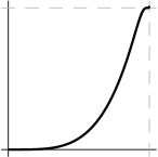
(a)

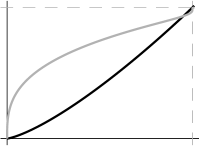
(b)

Figure 3: The diagonal: (a) $u$ as a function of $r=|\nabla u|\in[0,1]$. (b) $u(s\mathbbm{1})$ and $|\nabla u(s\mathbbm{1})|$ (gray) in arc-length parametrization $s\in[0,\sqrt{2}]$.

6 Deriving the solution

In this Section I shall give an heuristic explanation on how the formula (1.1) was obtained. No rigour is needed and I put the emphasise on the method and the ideas.

I shall take advantage of some known properties of the solution to (1.3) in the square $\overline{\Omega}=[0,2]^{2}$. Firstly, by repeatedly making odd reflections along the edges, one can tessellate the plane by a function that is infinity-harmonic in $\mathbb{R}^{2}$ except at coordinates $(m,n)$ where $m$ and $n$ are odd. Secondly, the bounds

$$1-\sqrt{(1-x)^{2}+(1-y)^{2}}\leq u(x,y)\leq\operatorname{dist}((x,y),\partial\Omega),$$

which follow by the comparison principle, determines both $u$ and $\nabla u$ on the medians of $\overline{\Omega}$, and – by extension – on the grid lines in $\mathbb{R}^{2}$ connecting the singularities $\{(m,n)\}$. In particular, the gradient is known on the boundary of the square

$$S:=\{[x,y]^{\top}\;|\;-1<x<1,\,-1<y<1\},$$

which is a prerequisite in order to use the hodograph transform.

I therefore consider the Dirichlet problem

$$\begin{cases}\Delta_{\infty}u=0\qquad&\text{in $S$},\\ u(t,1)=u(1,t)=t,\\ u(t,-1)=u(-1,t)=-t,&\text{for $-1\leq t\leq 1$.}\end{cases}$$ (6.1)

The restriction $u|_{\overline{\Omega}_{1}}$ will then be the solution of (2.2). This can also be seen by noting that the symmetry of the boundary conditions in (6.1) implies $u=0$ on the coordinate axis.

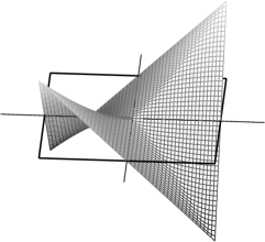
Figure 4: The graph of the solution to (6.1) over the square $\overline{S}=[-1,1]^{2}$.

The following ansatz is made: The gradient $\nabla u\colon S\to B$ to the solution of (6.1) is one-to-one and onto $B:=\left\{(p,q)\in\mathbb{R}^{2}\,|\,p^{2}+q^{2}<1\right\}$ – the unit disk. Denote by $\mathbf{f}\colon B\to S$ the inverse of $\nabla u$ and define $w\colon B\to\mathbb{R}$ as

$$w(\mathbf{p}):=\mathbf{p}^{\top}\mathbf{f}(\mathbf{p})-u(\mathbf{f}(\mathbf{p})).$$

If $\mathbf{f}$ is differentiable, then

$$\mathbf{p}=\nabla u^{\top}(\mathbf{f}(\mathbf{p}))\qquad\text{implies}\qquad I=\mathcal{H}u(\mathbf{f}(\mathbf{p}))\nabla f(\mathbf{p})$$

and

$$\nabla w(\mathbf{p}) =\mathbf{f}^{\top}(\mathbf{p})+\mathbf{p}^{\top}\nabla\mathbf{f}(\mathbf{p})-\nabla u(\mathbf{f}(\mathbf{p}))\nabla\mathbf{f}(\mathbf{p})=\mathbf{f}^{\top}(\mathbf{p}),$$

$$\mathcal{H}w(\mathbf{p}) =\nabla\mathbf{f}(\mathbf{p})=(\mathcal{H}u)^{-1}(\mathbf{f}(\mathbf{p})).$$

Thus,

$$0 =\nabla u(\mathbf{f}(\mathbf{p}))\mathcal{H}u(\mathbf{f}(\mathbf{p}))\nabla u^{\top}(\mathbf{f}(\mathbf{p}))$$

$$=\mathbf{p}^{\top}(\mathcal{H}w)^{-1}(\mathbf{p})\mathbf{p}$$

$$=[p,q]\begin{bmatrix}w_{pp}&w_{pq}\\ w_{pq}&w_{qq}\end{bmatrix}^{-1}\begin{bmatrix}p\\ q\end{bmatrix}$$

$$=\frac{1}{w_{pp}w_{qq}-w_{pq}^{2}}[p,q]\begin{bmatrix}w_{qq}&-w_{pq}\\ -w_{pq}&w_{pp}\end{bmatrix}\begin{bmatrix}p\\ q\end{bmatrix},$$

which leads to the linear homogeneous equation

$$0=p^{2}w_{qq}-2pqw_{pq}+q^{2}w_{pp}.$$ (6.2)

The equation is degenerate elliptic, as can be seen from writing the above as

$$0=[-q,p]\begin{bmatrix}w_{pp}&w_{pq}\\ w_{pq}&w_{qq}\end{bmatrix}\begin{bmatrix}-q\\ p\end{bmatrix}=\operatorname{tr}\left(A(\mathbf{p})\mathcal{H}w\right)$$

where $A\colon B\to\mathcal{S}^{2}_{+}$ is the one-rank matrix valued function

$$A(\mathbf{p}):=Q\mathbf{p}\mathbf{p}^{\top}Q^{\top},\qquad Q:=\begin{bmatrix}0&-1\\ 1&0\end{bmatrix}.$$ (6.3)

Since the domain of $w$ is the unit disk, it is natural to introduce polar coordinates. Define

$$W(r,\theta):=w(r\cos\theta,r\sin\theta).$$

Then $W_{\theta}=-w_{p}r\sin\theta+w_{q}r\cos\theta$ and

$$W_{\theta\theta} =-\left[-w_{pp}r\sin\theta+w_{pq}r\cos\theta\right]r\sin\theta$$

$$\quad{}-w_{p}r\cos\theta$$

$$\quad{}+\left[-w_{pq}r\sin\theta+w_{qq}r\cos\theta\right]r\cos\theta$$

$$\quad{}-w_{q}r\sin\theta$$

$$=q^{2}w_{pp}-2pqw_{pq}+p^{2}w_{qq}-pw_{p}-qw_{q}.$$

Since $rW_{r}=r(w_{p}\cos\theta+w_{q}\sin\theta)=pw_{p}+qw_{q}$ it follows that

$$rW_{r}+W_{\theta\theta}=0.$$ (6.4)

A separation of variables $W(r,\theta)=F(r)G(\theta)$ yields

$$\frac{rF^{\prime}(r)}{F(r)}=n^{2}=-\frac{G^{\prime\prime}(\theta)}{G(\theta)},\qquad n=0,1,2,\dots,$$

and suggests a solution on the form

$$W(r,\theta)=\sum_{n=0}^{\infty}r^{n^{2}}\left(A_{n}\cos(n\theta)+B_{n}\sin(n\theta)\right).$$ (6.5)

The boundary values of $w$ at $\partial B$ needs to be established. That is, the values $W(1,\theta)$ for $\theta\in[0,2\pi]$. Since $\nabla u=[1,0]$ at the upper boundary $\ell_{u}:=\{[t,1]^{\top}\;|\;-1<t<1\}\subseteq\partial S$, the gradient $\nabla u$ is certainly not invertible in the closure of $S$. Nevertheless, allowing $\mathbf{f}$ to be multivalued at $[1,0]^{\top}$ as $\mathbf{f}(1,0):=\ell_{u}$, still produces – with some goodwill – the single value

$$w(1,0) =[1,0]\mathbf{f}(1,0)-u(\mathbf{f}(1,0))$$

$$=[1,0]\begin{bmatrix}t\\ 1\end{bmatrix}-u(t,1)$$

$$=t-t=0$$

of $w$ at $[1,0]^{\top}$. The same calculations apply for the remaining three edges, but this strategy settles the values $W(1,k\pi/2)=0$, $k=0,1,2,3$, only at four boundary points.

We must examine the behaviour of $\nabla u$ at the corners of $S$. When $\mathbf{x}\in S$ approaches the corner point $[1,1]^{\top}$ we know from Corollary 10 in [LL19] that $|\nabla u(\mathbf{x})|\to 1$. Also, the gradient is continuous, and since $\nabla u(\ell_{u})=[1,0]$ on the upper boundary and $\nabla u(\ell_{r})=[0,1]$ on the right boundary $\ell_{r}:=\{[1,t]^{\top}\;|\;-1<t<1\}$, the gradient must take on all the ’intermediate’ values $\nabla u=[\cos\theta,\sin\theta]$, $0\leq\theta\leq\pi/2$, in some limit $\mathbf{x}\to[1,1]^{\top}$. We therefore consider $\nabla u$ as multivalued at $[1,1]^{\top}$. The ’inverse’ $\mathbf{f}$ is then constant $\mathbf{f}(\cos\theta,\sin\theta)=[1,1]^{\top}$ for $0\leq\theta\leq\pi/2$, and the boundary values for $W$ becomes

$$W(1,\theta) =w(\cos\theta,\sin\theta)$$

$$=[\cos\theta,\sin\theta]\mathbf{f}(\cos\theta,\sin\theta)-u(\mathbf{f}(\cos\theta,\sin\theta))$$

$$=[\cos\theta,\sin\theta]\begin{bmatrix}1\\ 1\end{bmatrix}-u(1,1)$$

$$=\cos\theta+\sin\theta-1,\qquad\theta\in[0,\pi/2].$$

I now continue around the square $S$ in a clock-wise manner in order to derive the boundary values also for $\theta\in[\pi/2,2\pi]$. At the lower edge $\ell_{l}:=\{[t,-1]^{\top}\;|\;-1<t<1\}$ we have $\nabla u=[-1,0]$, so near the corner $[1,-1]^{\top}$ the gradient sweeps $[\cos\theta,\sin\theta]$, $\pi/2\leq\theta\leq\pi$. We define $\mathbf{f}(\cos\theta,\sin\theta):=[1,-1]^{\top}$ for those values and get

$$W(1,\theta) =w(\cos\theta,\sin\theta)$$

$$=[\cos\theta,\sin\theta]\mathbf{f}(\cos\theta,\sin\theta)-u(\mathbf{f}(\cos\theta,\sin\theta))$$

$$=[\cos\theta,\sin\theta]\begin{bmatrix}1\\ -1\end{bmatrix}-u(1,-1)$$

$$=\cos\theta-\sin\theta+1,\qquad\theta\in[\pi/2,\pi].$$

Conducting the same analysis at the corner points $[-1,-1]^{\top}$ and $[-1,1]^{\top}$ will yield the values of $W$ all around the circle. Namely,

$$W(1,\theta)=\begin{cases}\cos\theta+\sin\theta-1,\qquad&\text{for $0\leq\theta\leq\pi/2$,}\\ \cos\theta-\sin\theta+1,\qquad&\text{for $\pi/2\leq\theta\leq\pi$,}\\ -\cos\theta-\sin\theta-1,\qquad&\text{for $\pi\leq\theta\leq 3\pi/2$,}\\ -\cos\theta+\sin\theta+1,\qquad&\text{for $3\pi/2\leq\theta\leq 2\pi$.}\end{cases}$$ (6.6)

Note that $W(1,k\pi/2)=0$ for integers $k$, as it should. The function is thus well defined and continuous. In fact, its derivative is

$$W_{\theta}(1,\theta)=|\cos\theta|-|\sin\theta|$$

for all $\theta$. As this function is continuous, even, and $\pi$-periodic, it follows that $W(1,\theta)$ is $C^{1}$, odd, and $\pi$-periodic.

The Fourier series of $|\cos\theta|$ and $|\sin\theta|$ can be calculated to

$$|\cos\theta|=\frac{2}{\pi}+\frac{4}{\pi}\sum_{n=1}^{\infty}\frac{(-1)^{n-1}}{4n^{2}-1}\cos(2n\theta),\quad|\sin\theta|=\frac{2}{\pi}-\frac{4}{\pi}\sum_{n=1}^{\infty}\frac{1}{4n^{2}-1}\cos(2n\theta),$$

so

$$W_{\theta}(1,\theta) =|\cos\theta|-|\sin\theta|$$

$$=\frac{4}{\pi}\sum_{n=1}^{\infty}\frac{(-1)^{n-1}+1}{4n^{2}-1}\cos(2n\theta)$$

$$=\frac{8}{\pi}\sum_{n=1}^{\infty}\frac{\cos(2(2n-1)\theta)}{4(2n-1)^{2}-1}$$

$$=\frac{8}{\pi}\sum_{n=1}^{\infty}\frac{\cos(m_{n}\theta)}{m_{n}^{2}-1}$$

where $m_{n}=4n-2$. From (6.5) it follows that $W_{\theta}(r,\theta)=\frac{8}{\pi}\sum_{n=1}^{\infty}\frac{r^{m_{n}^{2}}}{m_{n}^{2}-1}\cos(m_{n}\theta)$ and

$$w(r\cos\theta,r\sin\theta)=W(r,\theta)=\frac{8}{\pi}\sum_{n=1}^{\infty}\frac{r^{m_{n}^{2}}}{(m_{n}^{2}-1)m_{n}}\sin(m_{n}\theta).$$

There is no integration constant because the average of $W(1,\theta)$ is zero. This is important. The strategy would not have worked if the hodograph transform is taken over $\Omega_{1}$ alone.

When transforming back and letting $\mathbf{g}\colon S\to B$ be the inverse of $\nabla w^{\top}=\mathbf{f}$ – that is, $\mathbf{g}(\mathbf{x})=\nabla u^{\top}(\mathbf{x})$. Then $\mathbf{f}(\mathbf{p})=\mathbf{x}$ if and only if $\mathbf{p}=\mathbf{g}(\mathbf{x})$ and the identity $w(\mathbf{p})=\mathbf{p}^{\top}\mathbf{f}(\mathbf{p})-u(\mathbf{f}(\mathbf{p}))$ yields

$$u(\mathbf{x})=\mathbf{x}^{\top}\mathbf{g}(\mathbf{x})-w(\mathbf{g}(\mathbf{x})).$$ (6.7)

Finally, one may observe that this is a critical value of the function

$$\begin{bmatrix}r\\ \theta\end{bmatrix}=\mathbf{r}\mapsto f_{\mathbf{x}}(\mathbf{r}):=\mathbf{x}^{\top}\Phi(\mathbf{r})-w(\Phi(\mathbf{r})),\qquad\Phi(r,\theta)=\begin{bmatrix}r\cos\theta\\ r\sin\theta\end{bmatrix}.$$

Indeed, the critical point of $f_{\mathbf{x}}$ is $\mathbf{r}$ such that $\nabla w(\Phi(\mathbf{r}))=\mathbf{x}^{\top}$. Equivalently, $\Phi(\mathbf{r})=\mathbf{g}(\mathbf{x})$. Plugging this value back into $f_{\mathbf{x}}$, yields $u(\mathbf{x})$. When restricted to $0\leq\theta\leq\pi/2$, the graph of $f_{\mathbf{x}}$ is a saddle and I therefore assumed that the critical point is a minimax for every parameter $\mathbf{x}\in\Omega_{1}$.

It is possible that the approach taken can serve as a general method to construct solutions of $\Delta_{\infty}u=0$. Note that (6.7) should be $\infty$-harmonic for any particular solution $w$ of the hodograph equation (6.2) provided $\nabla w$ is locally invertible.

Acknowledgements:

The final draft of the manuscript was written at Institute Mittag-Leffler in Djursholm, Sweden, during the program Geometric Aspects of Nonlinear Partial Differential Equations in the fall of 2022. Supported by the Swedish Research Council under the grant no. 2016-06596.

A special thanks goes to Peter Lindqvist.

References

[Aro67]
Gunnar Aronsson.
Extension of functions satisfying Lipschitz conditions.
Ark. Mat., 6:551–561, 1967.
[Aro68]
Gunnar Aronsson.
On the partial differential equation .
Ark. Mat., 7:395–425, 1968.
[BBT20]
Farid Bozorgnia, Leon Bungert, and Daniel Tenbrinck.
The infinity laplacian eigenvalue problem: reformulation and a
numerical scheme, arXiv, 2020.
[BDM89]
T. Bhattacharya, E. DiBenedetto, and J. Manfredi.
Limits as of and related extremal
problems.
Number Special Issue, pages 15–68 (1991). 1989.
Some topics in nonlinear PDEs (Turin, 1989).
[Jen93]
Robert Jensen.
Uniqueness of Lipschitz extensions: minimizing the sup norm of the
gradient.
Arch. Rational Mech. Anal., 123(1):51–74, 1993.
[JLM99]
Petri Juutinen, Peter Lindqvist, and Juan J. Manfredi.
The -eigenvalue problem.
Arch. Ration. Mech. Anal., 148(2):89–105, 1999.
[JLM01]
Petri Juutinen, Peter Lindqvist, and Juan J. Manfredi.
The infinity Laplacian: examples and observations.
In Papers on analysis, volume 83 of Rep. Univ.
Jyväskylä Dep. Math. Stat., pages 207–217. Univ. Jyväskylä,
Jyväskylä, 2001.
[Lew77]
John L. Lewis.
Capacitary functions in convex rings.
Arch. Rational Mech. Anal., 66(3):201–224, 1977.
[LL19]
Erik Lindgren and Peter Lindqvist.
Infinity-harmonic potentials and their streamlines.
Discrete and Continuous Dynamical Systems, 39(8):4731–4746,
2019.
[LL21]
Erik Lindgren and Peter Lindqvist.
The gradient flow of infinity-harmonic potentials.
Advances in Mathematics, 378:107526, 2021.
[WW20]
E. T. Whittaker and G. N. Watson.
A course of modern analysis. An introduction to the general
theory of infinite processes and of analytic functions: with an account of
the principal transcendental functions.
Cambridge University Press, New York, 1920.
Third edition.
[Yu07]
Yifeng Yu.
Some properties of the ground states of the infinity Laplacian.
Indiana Univ. Math. J., 56(2):947–964, 2007.