KRF: Keypoint Refinement with Fusion Network for 6D Pose Estimation

Abstract

Existing refinement methods gradually lose their ability to further improve pose estimation methods’ accuracy. In this paper, we propose a new refinement pipeline, Keypoint Refinement with Fusion Network (KRF), for 6D pose estimation, especially for objects with serious occlusion. The pipeline consists of two steps. It first completes the input point clouds via a novel point completion network. The network uses both local and global features, considering the pose information during point completion. Then, it registers the completed object point cloud with corresponding target point cloud by Color supported Iterative KeyPoint (CIKP). The CIKP method introduces color information into registration and registers point cloud around each keypoint to increase stability. The KRF pipeline can be integrated with existing popular 6D pose estimation methods, e.g. the full flow bidirectional fusion network, to further improved their pose estimation accuracy. Experiments show that our method outperforms the state-of-the-art method from 93.9% to 94.4% on YCB-Video dataset and from 64.4% to 66.8% on Occlusion LineMOD dataset. Our source code is available at https://github.com/zhanhz/KRF.

I Introduction

6D object pose estimation is an essential component in many applications, such as robotic manipulation[4, 1], augmented reality[5], autonomous driving[6, 7] and so on, and has received extensive attention and research over the past decade. It is a quite challenging task because of sensor noise, occlusion between objects, varying lighting conditions and object symmetries.

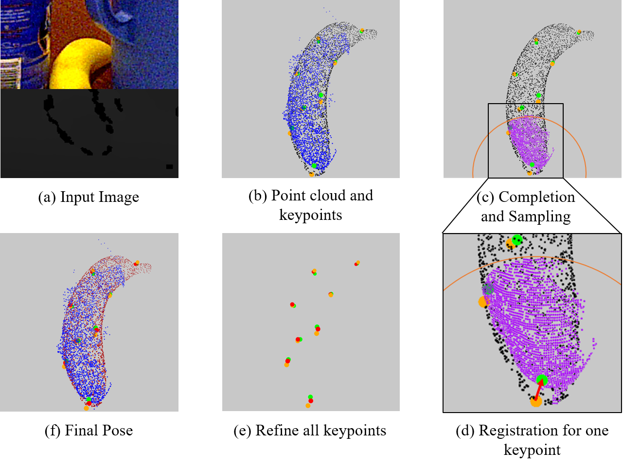
Figure 1: Pipeline of our method: With input RGBD image (a) (the bottom half shows the depth map) and initial pose, we transform the visible point cloud (shown in blue color, and black is the known object point cloud) to the object coordinate frame (b). After completing the visible point cloud, we take one of the mesh keypoints (shown in orange color, and green is the groundtruth keypoints) as center, collect points in completed point cloud within the sphere of radius $r$ (Purple), then register purple and black point cloud and get refined keypoints (Red) (c)-(e). Using the least squares fitting method to get final pose. The model transformed by the final pose is shown in (f) as red point cloud.

Traditional methods[8, 9] attempted to extract hand-craft feature from the correspondences between known RGB images and object mesh models. Such methods have limitations in heavy occlusion scenes or low-texture objects. Recently, with the explosive development of Deep Neural Networks (DNNs), these methods have been introduced into the 6D object pose estimation task and greatly improved the performance. Specifically, some methods[11, 3, 10] use DNNs to directly regress translation and rotation of each object. However, non-linearity of the rotation leads to poor generalization of these methods. More recently, works like[13, 14, 2] utilized DNNs to detect keypoints of each object, and then computed the 6D pose parameters with Perspective-n-Point (PnP) for 2D keypoints or Least Squares methods for 3D keypoints.

Though DNN methods can solve the problem with less time cost, they are still not able to achieve high accuracy due to error in segmentation or regression. To achieve higher accuracy, methods of pose refinement are proposed. The most common way to refine poses is Iterative Closest Point (ICP)[16]. Given an estimated pose, the method tries to find the nearest neighbor of each point of the source point cloud in the target point cloud as the corresponding point, then solves the optimal transformation iteratively. Besides, works like [22, 11] use DNNs to extract more features for better performance. However, with the development of pose estimation networks, performance improvement of these pose refinement methods become less and less. The reason is that the point cloud data is not fully utilized, and the color and point cloud data are not used in fusion. In this work, we proposed a novel completion network to complete visible point clouds to fully utilize the point cloud and RGB data, especially for seriously occluded objects. The encoder of the network was adapted from [15]. We add global information of the point cloud to improve its point completion performance. The decoder of the network followed [23] employs multistage point generation structure, and we use pose estimation branch as another decoder so that our network can complete point clouds with different orientations and positions. To use color and point data in registration, we proposed a framework of pose refinement that employs a novel method named Color supported Iterative KeyPoint (CIKP), which samples the point cloud around each keypoint, leveraging both RGB and point cloud information to refine object keypoints iteratively. Our Keypoint refinement with fusion (KRF) is a pipeline that combines our completion network, CIKP method and the full flow bidirectional fusion network [15]. We further conduct extensive experiments on YCB-Video[10] and Occlusion LineMOD[8] datasets to evaluate our method. Experimental results show that our method outperforms current state-of-the-art methods.

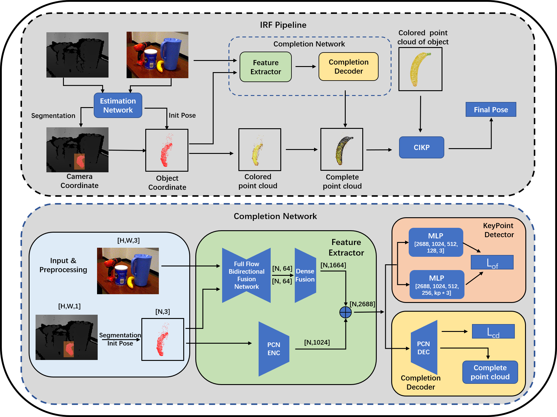
Figure 2: Inference process of KRF combining completion network and CIKP.

Our main contribution is threefold:

• A novel Iterative pose refinement method CIKP that using both RGB and depth information based on Least squares for keypoints.

• A novel point completion network that more suitable for pose refinement.

• KRF: A pipeline that combines our completion network, CIKP method and the full flow bidirectional fusion network.

Extensive experiments show that our KRF achieves the best result among existing methods.

II Related Works

II-A Pose Estimation

According to the optimization goal, pose estimation methods can be classified into holistic and keypoint-based methods. Holistic methods directly predict the 3D position and orientation of objects by the given RGB and/or depth images. Traditional template-based methods construct a rigid template for an object from different viewpoints and are used to compute the best-matched pose for the given image [24, 25]. Recently, some works made use of DNN to directly regress or classify the 6D pose of objects. PoseCNN [10] used a multi-stage network to predict pose. It first used Hough Voting to vote center location of objects, then direct regressed 3D rotation parameters. SSD-6D [12] first detected objects in the images and then classified them to their pose. DenseFusion [11] fused RGB and depth values at the per-pixel level, which has great influence on 6d pose estimation methods based on RGBD images. However, the non-linearity of the rotation makes it difficult for the loss function to converge.

In order to solve the above problem, keypoint-based methods were proposed. YOLO-6D [26] used the classic object detection model YOLO to predict 8 points and a center point of the bounding box of the object projected on the 2D image, then computed the 6D pose using the PnP algorithm. PVNet [13] tried to predict a unit vector to each keypoint for each pixel, then voted the 2D location for each keypoint and computed the final pose using the PnP algorithm. Similar to DenseFusion, PVN3D [14] used extra depth information to detect 3D keypoints via Hough Voting, then calculated 6D pose parameters with Least Squares method. To fully utilize RGB and depth data, FFB6D[15] proposed a new feature extraction network, in which fusion is applied at each of encoding and decoding layers.

II-B Pose Refinement

Most of the methods metioned above have considered to apply pose refinement techniques to further improve the accuracy of their results. The most commonly used method is ICP[16], but it only leverages the Euclidean distance between points. Some methods[18, 17] tried to change the optimization goal to accelerate the iterative process or improve the result. Others [19, 20] introduced a color space into ICP, which converges faster and get better results than 3D ICP methods.

Recently DNN-based approaches have also been considered to address the refinement issue. Given the initial pose and 3D object model, DeepIM[22] iteratively refined the pose by matching the rendered image against the observed image. Manhardt et al. [28] proposed a new visual loss that refines the pose by aligning object contours with the initial pose. Densefusion[11] also proposed their refinement network, which followed their main network with the original RGB features and the corresponding features of the transformed point cloud as input. With the development of pose estimation techniques, the improvement of pose refinement on estimation results becomes less and less, especially in methods using RGBD data. However, we noticed that researchers did not pay enough attention to the importance of refinement methods. Therefore, our goal in this paper is to combine the idea of ICP with deep learning and design a new pipeline of pose refinement to improve the estimation results.

III Our KRF Method

The task of 6D pose estimation is to predict the rigid transformation matrix $p\in SE(3)$, including a rotation matrix $R\in SO(3)$ and a translation matrix $T\in\mathbb{R}^{3}$. It transforms the object from its coordinate frame to the camera coordinate frame. Given an observed RGB image and a depth map, we first obtain the predicted pose and segmentation result of an object by the Pose Estimation Network. We select the FFB6D [15] to get the initial result. Then we utilize our KRF pipeline to compute a relative transformation $\Delta p\in SE(3)$ for correcting the result. Specifically, we first complete the visible point cloud by our completion network, then use the CIKP method to compute the refined pose. The summary of the inference process is shown in Fig. 2.

III-A Preprocessing

This part aims to get the keypoints, initial pose and point cloud of each object. First, we follow keypoint-based approaches [15, 14] to select $K$ keypoints on each object surface. Then, with an RGBD image as input, the Pose Estimation Network outputs the segmentation results and predicts the pose of each object in the image. Furthermore, we convert the given segmented depth map $D^{H_{s}\times W_{s}}$ to the point cloud of the target object $P_{c}^{3\times N}$, where $H_{s},W_{s}$ are the height and weight of the segmented depth map, and $N$ is the number of the point cloud. Finally, we convert the point cloud from the camera coordinate frame $P_{c}$ to the object coordinate frame $P_{o}$ by the given initial pose $R_{init}\in SO(3)$ and $T_{init}\in\mathbb{R}^{3}$.

$$P_{o}=R_{init}^{-1}(P_{c}-T_{init})$$ (1)

III-B Completion Network for Pose Refinement

The architecture of our network is illustrated in Fig. 2, which composes of a feature extractor, a completion decoder and a training-only keypoint detector.

Feature Extractor: To extract effective features from partial point cloud and make reasonable use of the RGB and depth fusion data, we combine the Full Flow Bidirectional Fusion Network [15], Dense Fusion module[11] and PCN encoder [23] as feature extractor. After preprocessing, we get the object point cloud with the predicted pose in its coordinate frame $P_{o}$. Then $P_{o}$ and observed RGB image $I^{H\times W\times 3}$ are fed into the Full Flow Bidirectional Fusion Network and Dense Fusion module to get local features of each point. Simultaneously, the global features are obtained from the PCN Decoder. Finally, local features and global features are concatenated as $F$.

Decoders: In this part, we output the dense point cloud for the CIKP. Since the input of CIKP is partial point clouds around each keypoint, it is essential to add keypoint decoder for the completion network, which enriches the detail around keypoints. Thus, the learned features $F$ are fed into 2 decoders: keypoint decoder for predicting keypoints and center offset, and PCN Decoder [23] for completing visible point cloud. Given a set of keypoints $P_{k}^{3\times K}$ and visible point cloud $P_{o}$, we define the translation offset from $i_{th}$ point $p_{i}\in P_{o}$ to $j_{th}$ keypoint $kp_{j}\in P_{k}$ as $of_{i}^{j}$. We supervise the keypoint detector module using $L_{of}$ loss:

$$L_{of}=\frac{1}{N}\sum_{i=1}^{N}\sum_{j=1}^{K}||of_{i}^{j}-of_{i}^{j*}||$$ (2)

Where $K$ is the number of keypoints, $of_{i}^{j*}$ is the groundtruth of translation offset. Note that $K=1$ if $L_{of}$ is used for predicting center point offset. We denote the loss of keypoints offset and center offset as $L_{kp}$ and $L_{c}$, respectively.

We supervise the completion decoder using $L_{cd}$ loss:

$$L_{cd}=\frac{1}{|P_{o}|}\sum_{x\in P_{o}}\min_{y\in P_{d}}||x-y||_{2}+\frac{1}{|P_{d}|}\sum_{y\in P_{d}}\min_{x\in P_{o}}||x-y||_{2}$$ (3)

where $P_{d}$ is the output dense point cloud. The overall loss $L$ is calculated as below:

$$L=\alpha L_{kp}+\beta L_{c}+\gamma L_{cd}$$ (4)

where $\alpha,\beta,\gamma$ represent the weights of different losses.

III-C Color Supported Iterative KeyPoint

Traditional registration algorithms for pose estimation only utilize the Euclidean distance between source point cloud and target point cloud. These methods are less stable since they only consider the registration of the entire point cloud without color information. Thus, we propose CIKP that iteratively refines each keypoint using the position and color information of each point.

We first define the distance between two colored points as in Eq. (5). Given two colored points $p_{1}$ and $p_{2}$, we divide them into a position space $x_{1},x_{2}\in\mathbb{R}^{3}$ and a color space $c_{1},c_{2}\in\mathbb{R}^{3}$ respectively. Note that $c_{1},c_{2}\in[0,1]$. The final distance between $p_{1},p_{2}$ is their distance in Euclidean space plus the distance in weighted color space. We stipulate that the closer the spatial distance, the higher the weight of the color distance. In addition, we set a threshold $\epsilon$ to keep weight within $(0,1]$, because the initial pose already has relatively high accuracy.

$$D_{1}=||x_{1}-x_{2}||_{2}$$ (5)

$$D_{2}=||c_{1}-c_{2}||_{2}$$

$$w=\max(\frac{D_{1}}{\epsilon},1)$$

$$D=D_{1}+\frac{1}{w}D_{2}$$

The process of CIKP is summarized in Alg. 1. The source point cloud $P_{s}$ is a colored point cloud of objects, and the target point cloud $P_{t}$ consists of visible colored point clouds and uncolored point clouds completed by our completion network, where $P_{s}$ is in the object coordinate frame, and $P_{t}$ is converted back to the camera coordinate frame. We first select a keypoint, take it as the center, and collect all points in the $P_{t}$ within the sphere of radius $r$, denoted by $S_{p}$. If $|S_{p}|$ is less than a threshold $m_{1}$, we keep its original state and select the next keypoint. And if $|S_{p}|$ is more than $m_{2}$, we randomly select $m_{2}$ points in $S_{p}$. Then for each $p_{t}\in S_{p}$, we find its closest point in $P_{s}$ denoted by $M$. If $p_{t}$ is colored, we use Eq. (5) to calculate distance, otherwise calculate their Euclidean distance directly. After that, we calculate the optimal translation transformation $T_{k}$ between the two point clouds and transform the selected keypoint with $T_{k}$. After all keypoints have been transformed, the refined pose is calculated using the Least Squares method. We repeat the above steps until the mean distance between corresponding points less than a threshold $\tau$ or reach the maximum number of iterations.

Input: source point cloud $P_{s}$, target point cloud $P_{t}$, keypoint set $S_{k}$, search radius $r$, threshold $m_{1},m_{2}$, initial rotation $R_{init}$ and transformation $T_{init}$

Output: refined rotation $R$ and translation $T$

Initialize : sampled point cloud set $S_{p}$, closest point set $M$, refined keypoint set $S_{kpr}$, source point cloud in camera coordinate frame $P_{a}$

1 $T\leftarrow T_{init}$

2$R\leftarrow R_{init}$

3while  not converged do

4       $P_{a}\leftarrow R\times P_{s}+T$

5      $S_{kpr}\leftarrow R\times S_{k}+T$

6      foreach  $i\leftarrow 1:n_{kp}$ do

7             $S_{p}\leftarrow\varnothing$

8            $M\leftarrow\varnothing$

9            foreach $p_{t}\in P_{t}$ do

10                   if $distXYZ(S_{kpr}[i],p_{t})<r$ then

11                         push $p_{t}$ into $S_{p}$

12                   end if

13                  

14             end foreach

15            if $|S_{p}|<m_{1}$ then

16                   continue

17             end if

18            if $|S_{p}|>m_{2}$ then

19                   Random select $m_{2}$ points in $S_{p}$

20             end if

21            foreach $p_{t}\in S_{p}$ do

22                   $p\leftarrow FindClosestPointInP_{a}(p_{t})$

23                  push $p$ into $M$

24             end foreach

25            

26            $T_{k}\leftarrow\underset{T_{k}}{\arg\min}\ \underset{j}{\sum}distXYZ(S_{p}[j],M[j]+T_{k})$

27            $S_{kpr}[i]\leftarrow S_{kpr}[i]+T_{k}$

28       end foreach

29      $[R,T]=\underset{R,T}{\arg\min}\ \underset{i}{\sum}distXYZ(R\times S_{k}[i]+T,S_{kpr}[i])$

30 end while

Algorithm 1 Color Supported Iterative KeyPoint

TABLE I: Result of 6D Pose Estimation on YCB-Video Dataset. The ADD-S and ADD(S) AUC are reported. Symmetric objects are in bold.

	DF[11]+iterative		PVN3D[14]		FFB6D[15]		DKS[34]		KRF
	ADD-S	ADD(S)	ADD-S	ADD(S)	ADD-S	ADD(S)	ADD-S	ADD(S)	ADD-S	ADD(S)
002_master_chef_can	96.4	73.2	96.0	80.8	96.4	80.7	96.4	81.5	96.5	81.7
003_cracker_box	95.8	94.1	96.0	94.5	96.4	95.0	96.5	95.1	96.7	95.6
004_sugar_box	97.6	96.5	97.1	95.5	97.7	96.8	97.8	96.9	98.0	97.3
005_tomato_soup_can	94.5	85.5	95.5	88.4	95.8	88.1	95.9	88.3	95.9	88.3
006_mustard_bottle	97.3	94.7	97.8	97.0	98.1	97.6	98.2	97.7	98.4	98.0
007_tuna_fish_can	97.1	81.9	96.3	90.1	97.2	91.3	97.3	92.1	97.3	92.2
008_pudding_box	96.0	93.3	96.9	95.3	96.3	93.1	96.4	93.4	96.7	94.2
009_gelatin_box	98.0	96.7	97.8	96.2	97.8	95.8	97.8	95.9	98.1	96.2
010_potted_meat_can	90.7	83.6	93.0	88.6	92.6	89.8	92.9	90.3	92.9	90.0
011_banana	96.2	83.3	91.3	93.5	97.4	94.9	97.3	94.4	97.8	95.8
019_pitcher_base	97.5	96.9	96.9	95.6	97.7	97.0	97.8	97.2	97.9	97.4
021_bleach_cleanser	95.9	89.9	96.3	93.6	96.5	93.7	96.5	93.8	96.9	94.5
024_bowl	89.5	89.5	89.4	89.4	95.8	95.8	96.5	96.5	96.6	96.6
025_mug	96.7	88.9	97.4	95.0	97.5	95.3	97.6	95.6	98.2	96.2
035_power_drill	96.0	92.7	96.6	95.1	97.3	96.2	97.3	96.3	98.2	97.2
036_wood_block	92.8	92.8	90.4	90.4	93.1	93.1	93.6	93.6	94.3	94.3
037_scissors	92.0	77.9	96.5	92.7	98.1	97.1	98.1	97.1	98.1	97.1
040_large_marker	97.6	93.0	96.8	91.7	96.9	90.0	97.0	90.2	98.0	90.5
051_large_clamp	72.5	72.5	90.5	90.5	96.8	96.8	97.1	97.1	96.7	96.7
052_extra_large_clamp	69.9	69.9	87.1	87.1	96.1	96.1	96.1	96.1	95.6	95.6
061_foam_brick	92.0	92.0	96.8	96.8	97.6	97.6	97.9	97.9	97.7	97.7
Average	93.0	87.6	95.1	92.3	96.6	93.9	96.7	94.1	96.9	94.4
Following PoseCNN	93.2	86.1	95.2	91.5	96.6	92.9	—	—	96.8	93.4

TABLE II: Result of 6D Pose Estimation on Occlusion LineMOD Dataset. The ADD-0.1 metirc is reported. Symmetric objects are in bold.

	Pix2Pose[37]	PVNet[13]	HybridPose[36]	DeepIM[22]	PVN3D[14]	FFB6D[15]	KRF
ape	22.0	15.8	20.9	59.2	58.2	57.3	57.7
can	44.7	63.3	75.3	63.5	83.2	80.9	83.4
cat	22.7	16.7	24.9	26.2	37.5	36.6	38.3
driller	44.7	65.7	70.2	55.6	78.7	76.6	79.8
duck	15.0	25.2	27.9	52.4	45.1	62.0	61.4
eggbox	25.2	50.2	52.4	63.0	60.3	56.6	59.7
glue	32.4	49.6	53.8	71.7	68.2	64.1	66.7
holepuncher	49.5	39.7	54.2	52.5	69.1	80.7	87.4
Average	32.0	40.8	47.5	55.5	62.5	64.4	66.8

IV Experiment

IV-A Datasets

We evaluate our proposed method on two benchmark datasets.

YCB-Video

The YCB-Video dataset consists of 21 objects selected from the YCB object set. It contains 92 videos captured by RGBD cameras, and each video consists of 3-9 objects, leading to totally over 130K frames. We followed previous works [10, 15, 11] to split them into the training and testing sets. The training set also includes 80,000 synthetic images released by [10].

Occlusion LineMOD

The Occlusion LineMOD dataset [8] is re-annotated from the Linemod [9] dataset, to compensate for its lack of occlusion. Unlike the LineMOD dataset, each frame in the Occlusion LineMOD dataset contains multiple heavily occluded objects, making it more challenging. We follow the previous work [10] to split the training and testing sets and generate synthetic images for training.

IV-B Evaluation Metrics

We use the average distance ADD and average distance for symmetric objects ADD-S as metrics. Given the set of object point cloud $\mathcal{O}$, the ground truth pose $[R^{*},T^{*}]$ and predicted pose $[R,T]$, ADD and ADD-S are defined as follows:

$$ADD=\frac{1}{m}\underset{x\in\mathcal{O}}{\sum}||(Rx+T)-(R^{*}x+T^{*})||$$ (6)

$$ADD\text{-}S=\frac{1}{m}\underset{x_{1}\in\mathcal{O}}{\sum}\underset{x_{2}\in\mathcal{O}}{\min}||(Rx_{1}+T)-(R^{*}x_{2}+T^{*})||$$ (7)

In the YCB-Video dataset, we report the area under ADD-S and ADD(S) curve (AUC) following [10] and set the maximum threshold of AUC to be 0.1m. The ADD(S) computes ADD-S for symmetric objects and ADD for others. In the Occlusion LineMOD dataset, we report the accuracy of ADD(S) distance less than 10% of the diameter of the object (ADD(S)-0.1).

IV-C Implementation Details

All experiments are deployed on a PC with Intel E5-2640-v4 CPU and NVIDIA RTX2080Ti GPU. FFB6D [15] is chosen as the Estimation Network. In Full Flow Bidirectional Fusion Network, a PSPNet [30] with a ResNet34 [32] pretrained on ImageNet [31] is applied to extract features of RGB images. We randomly sample 2,048 points for each object and apply RandLA-Net to extract the geometry feature of the point clouds. These features then fused by DenseFusion [11]. The PCN-ENC block consists of two stacks of PointNet to extract the global feature of the point clouds. The keypoint detector block consists of two MLPs whose details are shown in Fig. 2. We follow [23] to employ a multi-stage structure in PCN-DEC to output coarse point cloud (2,048 points) and detailed point cloud (8,192 points). We set $\alpha=\beta=1,\gamma=10$ in Eq. (4) and search radius $r$ to be 0.7 times the radius of the selected object. For keypoints, we apply the SIFT-FPS [15] algorithm to select $K=8$ keypoints for each target object.

IV-D Evaluation on YCB-Video and Occlusion LineMOD

Table I shows the evaluation of all the 21 objects in the YCB-Video dataset, and some qualitative results are shown in Fig 3. The results in Table I show that using FFB6D as a base estimation network, our method outperforms DKS by 0.3% and the original results by 0.5% on the ADD(S) metric. Besides, our method also gets the best result for most objects. Furthermore, results show that our method has obvious advantages in objects with regular geometric and rich textures (e.g. cracker_box, pudding_box) and distinct geometries (e.g. banana, mug, power_drill). However, our method is inferior to FFB6D on the results of large_clamp and extra_large_clamp, and we find the degradation of performance comes from segmentation. In fact, accurately segmenting these two objects is challenging since they have the same appearance but different sizes. In summary, our keypoint-by-keypoint refinement strategy enables our method to achieve better results.

Table II shows the evaluation of 8 objects in Occlusion LineMOD dataset. The table shows that our method achieves the best overall results and outperforms FFB6D by 2.4%. Compared to Tabel I, our method achieves a larger improvement on Occlusion LineMOD dataset, indicating that our method is more robust in occluded environments. However, there is a large margin between our method and DeepIM method in eggbox and glue, mainly due to the poor segmentation accuracy.

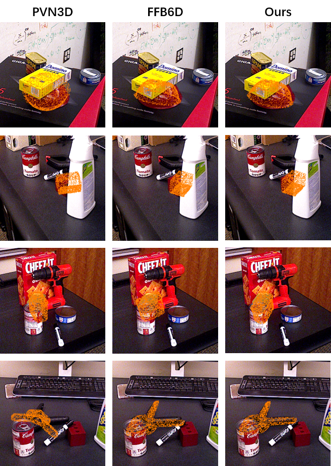
Figure 3: Qualitative results on the YCB-Video Dataset.

TABLE III: Ablation study for Completion Network on YCB-Video dataset. KPDEC means keypoint detector block.

FFB	DF	KPDEC	ADD(S)
			92.9
✓			93.1
✓		✓	93.2
✓	✓	✓	93.4

TABLE IV: Ablation study for CIKP on YCB-Video dataset. KP:refinement by keypoints. CN:using completion network

	Init Pose	KP	Color	CN	PCN[23]	ADD(S)
FFB6D [15]	92.9				✓	92.7
						92.9
		✓				93.1
			✓			93.0
		✓	✓		✓	92.9
		✓	✓			93.2
		✓		✓		93.2
		✓	✓	✓		93.4

TABLE V: Ablation study for CIKP using PVN3D as Estimation Network on YCB-Video dataset.

	Init Pose	KP	Color	CN	ADD(S)
PVN3D [14]	91.5				91.9
		✓			92.1
		✓	✓		92.2
		✓		✓	92.4
		✓	✓	✓	92.5

IV-E Ablation Study

In this part, we conduct ablation experiments to test the contribution of each part of our method.

Completion Network

Table III reported the ablation study result for Completion Network. FFB means the Full Flow Bidirectional Fusion block. DF means Dense Fusion block. KPDEC means keypoint detector block, which is only used in the training process. As summarized in Table III, all of the above blocks are beneficial to performance. This is because the FFB block can fully fuse RGB and point cloud features of objects in each pixel, and the DF block can match the number of channels of local and global features. Furthermore, training with the keypoint detector block allows the features to incorporate some information about the pose of objects, which is also beneficial to performance.

CIKP

Table IV and V reported the ablation study for CIKP method with initial poses given by two different methods. KP means refining pose keypoint-by-keypoint. Color means using color information. CN means using our completion network. In this ablation study, we also report the refinement results using PVN3D as Estimation Network. Experiment shows that refining pose by each keypoint can increase the stability of the refinement method, colored points can provide more information to register two point clouds, and the completed target point cloud can fully utilize the point cloud data. It can be observed that each part has a relatively consistent contribution to the final result, which verifies the necessity of each step of CIKP. In Table IV, we also compare our completion network and PCN [23]. Results show that after adding PCN, it was worse than before, demonstrating that our improvement on the completion network for refinement is meaningful.

V Conclusions

In this paper, we proposed a pose estimation pipeline KRF that combines estimation methods, a point cloud completion network and a Color Iterative KeyPoint method. Experiments show that all novel components are effective, and our method outperforms the state-of-the-art methods on YCB-Video and Occlusion LineMOD datasets.

References

- [1] J. Tremblay, T. To, B. Sundaralingam, Y. Xiang, D. Fox, and S. Birchfield, “Deep object pose estimation for semantic robotic grasping of household objects,” arXiv preprint arXiv:1809.10790, 2018.
- [2] L. Zeng, W. J. Lv, X. Y. Zhang, and Y. J. Liu, “ParametricNet: 6DoF Pose Estimation Network for Parametric Shapes in Stacked Scenarios,” in 2021 IEEE International Conference on Robotics and Automation (ICRA), 2021, pp. 772–778.
- [3] Z. Dong, S. Liu, T. Zhou, H. Cheng, L. Zeng, X. Yu, and H. Liu, “PPR-Net:Point-wise Pose Regression Network for Instance Segmentation and 6D Pose Estimation in Bin-picking Scenarios,” in 2019 IEEE/RSJ International Conference on Intelligent Robots and Systems (IROS), 2019, pp. 1773–1780.
- [4] M. Zhu, K. G. Derpanis, Y. Yang, S. Brahmbhatt, M. Zhang, C. Phillips, M. Lecce, and K. Daniilidis, “Single image 3d object detection and pose estimation for grasping,” in 2014 IEEE International Conference on Robotics and Automation (ICRA). IEEE, 2014, pp. 3936–3943.
- [5] E. Marchand, H. Uchiyama, and F. Spindler, “Pose estimation for augmented reality: a hands-on survey,” IEEE Transactions on Visualization and Computer Graphics, vol. 22, no. 12, pp. 2633–2651, 2015.
- [6] X. Chen, H. Ma, J. Wan, B. Li, and T. Xia, “Multi-view 3d object detection network for autonomous driving,” in Proceedings of the IEEE Conference on Computer Vision and Pattern Recognition, 2017, pp. 1907–1915.
- [7] D. Xu, D. Anguelov, and A. Jain, “PointFusion: Deep Sensor Fusion for 3D Bounding Box Estimation,” in Proceedings of the IEEE Conference on Computer Vision and Pattern Recognition (CVPR), June 2018.
- [8] E. Brachmann, A. Krull, F. Michel, S. Gumhold, J. Shotton, and C. Rother, “Learning 6d object pose estimation using 3d object coordinates,” in European Conference on Computer Vision. Springer, 2014, pp. 536–551.
- [9] S. Hinterstoisser, V. Lepetit, S. Ilic, S. Holzer, G. Bradski, K. Konolige, and N. Navab, “Model based training, detection and pose estimation of texture-less 3d objects in heavily cluttered scenes,” in Asian Conference on Computer Vision. Springer, 2012, pp. 548–562.
- [10] Y. Xiang, T. Schmidt, V. Narayanan, and D. Fox, “PoseCNN: A convolutional neural network for 6d object pose estimation in cluttered scenes,” arXiv preprint arXiv:1711.00199, 2017.
- [11] C. Wang, D. Xu, Y. Zhu, R. Martín-Martín, C. Lu, L. Fei-Fei, and S. Savarese, “Densefusion: 6d object pose estimation by iterative dense fusion,” in Proceedings of the IEEE/CVF Conference on Computer Vision and Pattern Recognition, 2019, pp. 3343–3352.
- [12] W. Kehl, F. Manhardt, F. Tombari, S. Ilic, and N. Navab, “SSD-6D: Making rgb-based 3d detection and 6d pose estimation great again,” in Proceedings of the IEEE International Conference on Computer Vision, 2017, pp. 1521–1529.
- [13] S. Peng, Y. Liu, Q. Huang, X. Zhou, and H. Bao, “PVNet: Pixel-wise voting network for 6dof pose estimation,” in Proceedings of the IEEE/CVF Conference on Computer Vision and Pattern Recognition, 2019, pp. 4561–4570.
- [14] Y. He, W. Sun, H. Huang, J. Liu, H. Fan, and J. Sun, “PVN3D: A deep point-wise 3d keypoints voting network for 6dof pose estimation,” in Proceedings of the IEEE/CVF Conference on Computer Vision and Pattern Recognition, 2020, pp. 11 632–11 641.
- [15] Y. He, H. Huang, H. Fan, Q. Chen, and J. Sun, “FFB6D: A full flow bidirectional fusion network for 6d pose estimation,” in Proceedings of the IEEE/CVF Conference on Computer Vision and Pattern Recognition, 2021, pp. 3003–3013.
- [16] P. J. Besl and N. D. McKay, “Method for registration of 3-d shapes,” in Sensor Fusion IV: Control Paradigms and Data Structures, vol. 1611. International Society for Optics and Photonics, 1992, pp. 586–606.
- [17] A. Segal, D. Haehnel, and S. Thrun, “Generalized-ICP.” in Robotics: Science and Systems, vol. 2, no. 4. Seattle, WA, 2009, p. 435.
- [18] J. Serafin and G. Grisetti, “NICP: Dense normal based point cloud registration,” in 2015 IEEE/RSJ International Conference on Intelligent Robots and Systems (IROS). IEEE, 2015, pp. 742–749.
- [19] H. Men, B. Gebre, and K. Pochiraju, “Color point cloud registration with 4D ICP algorithm,” in 2011 IEEE International Conference on Robotics and Automation. IEEE, 2011, pp. 1511–1516.
- [20] M. Korn, M. Holzkothen, and J. Pauli, “Color supported generalized-ICP,” in 2014 International Conference on Computer Vision Theory and Applications (VISAPP), vol. 3. IEEE, 2014, pp. 592–599.
- [21] T. Wan, S. Du, Y. Xu, G. Xu, Z. Li, B. Chen, and Y. Gao, “RGB-D point cloud registration via infrared and color camera,” Multimedia Tools and Applications, vol. 78, no. 23, pp. 33 223–33 246, 2019.
- [22] Y. Li, G. Wang, X. Ji, Y. Xiang, and D. Fox, “DeepIM: Deep iterative matching for 6d pose estimation,” in Proceedings of the European Conference on Computer Vision (ECCV), 2018, pp. 683–698.
- [23] W. Yuan, T. Khot, D. Held, C. Mertz, and M. Hebert, “PCN: Point completion network,” in 2018 International Conference on 3D Vision (3DV). IEEE, 2018, pp. 728–737.
- [24] Z. Cao, Y. Sheikh, and N. K. Banerjee, “Real-time scalable 6dof pose estimation for textureless objects,” in 2016 IEEE International Conference on Robotics and Automation (ICRA). IEEE, 2016, pp. 2441–2448.
- [25] S. Hinterstoisser, C. Cagniart, S. Ilic, P. Sturm, N. Navab, P. Fua, and V. Lepetit, “Gradient response maps for real-time detection of textureless objects,” IEEE Transactions on Pattern Analysis and Machine Intelligence, vol. 34, no. 5, pp. 876–888, 2011.
- [26] B. Tekin, S. N. Sinha, and P. Fua, “Real-time seamless single shot 6d object pose prediction,” in Proceedings of the IEEE Conference on Computer Vision and Pattern Recognition, 2018, pp. 292–301.
- [27] K. Gupta, L. Petersson, and R. Hartley, “Cullnet: Calibrated and pose aware confidence scores for object pose estimation,” in Proceedings of the IEEE/CVF International Conference on Computer Vision Workshops, 2019, pp. 0–0.
- [28] F. Manhardt, W. Kehl, N. Navab, and F. Tombari, “Deep model-based 6d pose refinement in rgb,” in Proceedings of the European Conference on Computer Vision (ECCV), September 2018.
- [29] S. Hinterstoisser, S. Holzer, C. Cagniart, S. Ilic, K. Konolige, N. Navab, and V. Lepetit, “Multimodal templates for real-time detection of texture-less objects in heavily cluttered scenes,” in 2011 International Conference on Computer Vision. IEEE, 2011, pp. 858–865.
- [30] H. Zhao, J. Shi, X. Qi, X. Wang, and J. Jia, “Pyramid scene parsing network,” in Proceedings of the IEEE Conference on Computer Vision and Pattern Recognition, 2017, pp. 2881–2890.
- [31] J. Deng, W. Dong, R. Socher, L.-J. Li, K. Li, and L. Fei-Fei, “Imagenet: A large-scale hierarchical image database,” in 2009 IEEE Conference on Computer Vision and Pattern Recognition. IEEE, 2009, pp. 248–255.
- [32] K. He, X. Zhang, S. Ren, and J. Sun, “Deep residual learning for image recognition,” in Proceedings of the IEEE Conference on Computer Vision and Pattern Recognition, 2016, pp. 770–778.
- [33] Q. Hu, B. Yang, L. Xie, S. Rosa, Y. Guo, Z. Wang, N. Trigoni, and A. Markham, “Randla-net: Efficient semantic segmentation of large-scale point clouds,” in Proceedings of the IEEE/CVF Conference on Computer Vision and Pattern Recognition, 2020, pp. 11 108–11 117.
- [34] H. Sun, T. Wang, and E. Yu, “A dynamic keypoint selection network for 6dof pose estimation,” Image and Vision Computing, vol. 118, p. 104372, 2022.
- [35] V. Badrinarayanan, A. Kendall, and R. Cipolla, “Segnet: A deep convolutional encoder-decoder architecture for image segmentation,” IEEE Transactions on Pattern Analysis and Machine Intelligence, vol. 39, no. 12, pp. 2481–2495, 2017.
- [36] C. Song, J. Song, and Q. Huang, “Hybridpose: 6d object pose estimation under hybrid representations,” in Proceedings of the IEEE/CVF Conference on Computer Vision and Pattern Recognition, 2020, pp. 431–440.
- [37] K. Park, T. Patten, and M. Vincze, “Pix2pose: Pixel-wise coordinate regression of objects for 6d pose estimation,” in Proceedings of the IEEE/CVF International Conference on Computer Vision, 2019, pp. 7668–7677.