The Trajectory PHD Filter for
Coexisting Point and Extended Target Tracking

Abstract

This paper develops a general trajectory probability hypothesis density (TPHD) filter, which uses a general density for target-generated measurements and is able to estimate trajectories of coexisting point and extended targets. First, we provide a derivation of this general TPHD filter based on finding the best Poisson posterior approximation by minimizing the Kullback-Leibler divergence, without using probability generating functionals. Second, we adopt an efficient implementation of this filter, where Gaussian densities correspond to point targets and Gamma Gaussian Inverse Wishart densities for extended targets. The $L$-scan approximation is also proposed as a simplified version to mitigate the huge computational cost. Simulation and experimental results show that the proposed filter is able to classify targets correctly and obtain accurate trajectory estimation.

I Introduction

Autonomous vehicles promise the possibility of fundamentally changing the transportation industry, with an increase in both highway capacity and traffic flow [1]. It is required to simultaneously extract the environmental information that incorporates dynamic as well as static objects through road infrastructure and other vehicles [2, 3, 4, 5]. Accordingly, the multi-target tracking (MTT) approaches are widely used for estimating the states and number of dynamic targets, which may appear, move and disappear, given noisy sensor measurements in time sequence[6].

There are two main kinds of approaches to solve MTT problems. The first category is based on random vectors, such as the joint probabilistic data association (JPDA) filter [7, 8] and the multiple hypotheses tracking (MHT) [6, 9]. The second category is based on random finite set (RFS)[10, 11, 12]. Among them, RFS-based algorithms have been proved to possess an excellent tracking performance in various scenarios[13, 14, 15, 16, 17]. The PHD filter, known for its low computational burden among all RFS based filters, possesses a high efficiency in solving real time tracking problem[18, 19]. It propagates the first-order multi-target moments[10], also called intensity, through prediction and update step. The PHD filter can also be derived by propagating a Poisson multi-target density through the filtering recursion, obtained via Kullback-Leibler divergence (KLD) minimization[10, 20].

In MTT, an important topic is to obtain accurate trajectory estimates and mitigate trajectory fragmentation [21]. Recently, calculating the posterior over a set of trajectories [22, 23, 24, 25, 26] or a (labeled) multi-target state sequence [21] provide an efficient approach to the above requirements. Among these approaches, the trajectory PHD (TPHD) filter [23] establishes trajectories from first principles using trajectory RFSs. The TPHD filter propagates the best Poisson multi-trajectory density under the standard point target dynamic and measurement models [20]. The Gaussian mixture is proposed to obtain a closed-form solution of the TPHD filter. Other trajectory-based filters for point targets are the trajectory multi-Bernoulli filter, trajectory PMBM filter and trajectory PMB filter.[25, 24]. Compared to filters based on sets of targets, filters based on sets of trajectories contain all information to answer trajectory-related questions, which are of major importance in autonomous vehicles and smart traffic systems.

In order to develop Bayesian filters, we need to model the distribution of the measurements given the targets as well as clutter. There are two main types of modeling for target-generated measurements: the point target model and the extended target model. In general, a point model is applied for the target measurement that is smaller than the sensor resolution, given its size and distance from the sensor[18, 13, 27].

Conversely, a target may generate more than one measurement if multiple resolution cells of the sensor are occupied by a single target, which is referred to as the extended target[28]. The Poisson point process (PPP) is widely used in the measurement model for an extended target[29], i.e., a Poisson distributed random number of measurements are generated, distributed around an extended target at each time step. There are extended target filters for sets of targets [30, 31, 32, 33, 34, 28] and also sets of trajectories [35, 36]. Except for extracting dynamic target state information, the mean number of generated measurements from an extended target or the size of the target are also modeled in these filters. Besides, there are also approaches for Bayesian smoothing of target extent based on random matrix model[37, 36].

There are many applications in which it is important to develop models and algorithms for simultaneous point and extended targets [12, 38]. For example, in a self-driving vehicle application, pedestrians may be modeled as point targets while some vehicles are taken as extended targets. Besides, the distinction between point and extended targets may also depend on the distance.

Figure 1: Diagram of the proposed TPHD filter, with Poisson birth model and no spawning. This filter propagates a Poisson density on the set of alive trajectories, whose form is kept in the prediction. Bayes’ rule provides a Poisson multi-Bernoulli density that is projected back to Poisson via minimizing the KLD.

In this paper, we propose a TPHD filter for coexisting point and extended targets. This filter combines the computational efficiency of PHD filters, with the ability to estimate trajectories from first principles in situations with point and extended targets. In particular, the contributions of this paper are:

1. A derivation of the TPHD filter update for general target-generated measurement density and PPP clutter is proposed based on direct KLD minimization (see Fig. 1). The corresponding derivation for the general PHD filter was derived using probability generating functionals (PGFLs) [39, 11]. Therefore, the proposed derivation increases the accessibility of the proof to a wider audience.

2. We apply the general TPHD filter for tracking coexisting point and extended targets. The implementation is provided for a linear Gaussian model for point targets [40, 18, 23] and a Gamma Gaussian Inverse Wishart (GGIW) model for extended targets [32, 33, 28, 34].

3. Simulation and real-world experimental results demonstrate the general TPHD filter can achieve excellent performance in tracking both point and extended target.

The structure of this paper is organized as follows. In Section II, theoretical background and the update and prediction steps of the general TPHD filter are provided. The implementation is given in Section III. In Section IV, we give the simulation and experimental results of the proposed filter. Finally, conclusion are drawn in Section IV,

II The General TPHD Filter

In this section, the recursion steps of the general TPHD filter are provided. The main idea is to use a general likelihood for target-generated measurements in the update step. We define sets of trajectories, the Bayesian filtering recursion for sets of trajectories, and provide the update and prediction steps of the general TPHD filter.

II-A Sets of Trajectories

The trajectory state $X=(t,x^{1:i})$ consists of a finite sequence of target states $x^{1:i}=(x^{1},...,x^{i})$ that starts at the time step $t$ with length $i$, where $x^{i}\in\mathbb{R}^{n_{x}}$ [23]. For $k$ denoting the current time step and a trajectory $(t,x^{1:i})$ that exists from time $t$ to $t+i-1$, the variable $(t,i)$ belongs to the set $\mathbb{I}_{k}=\{(t,i):1\leq t\leq k\leavevmode\nobreak\ \text{and}\leavevmode\nobreak\ 1\leq i\leq k-t+1\}$. Therefore, a single trajectory up to the time step $k$ is defined in the space $\mathbb{T}_{k}=\uplus_{(t,i)\in\mathbb{I}_{k}}\{t\}\times\mathbb{R}^{i\times n_{x}}$, where $\uplus$ denotes the disjoint union, $\times$ denotes a Cartesian product, and $n_{x}$ represents the dimension of target state. Supposing there are $N^{k}$ trajectories at time $k$, the set of trajectories is denoted as

$$\mathbf{X}_{k}=\{X_{1},...,X_{N^{k}}\}\in\mathcal{F}(\mathbb{T}_{k}),$$ (1)

where $\mathcal{F}(\mathbb{T}_{k})$ represents the set of all finite subsets of $\mathbb{T}_{k}$.

II-B Bayesian Filtering Recursion

Given the posterior multi-trajectory density $\pi_{k-1}(\cdot)$ on the set of trajectories at time $k-1$ and the set of measurements $\mathbf{z}_{k}$ at time $k$, the posterior density $\pi_{k}(\cdot)$ is obtained by using the Bayes’ recursion [26]

$$\pi_{k|k-1}\left(\mathbf{X}_{k}\right)= \int{\phi\left({\mathbf{X}_{k}|\mathbf{X}_{k-1}}\right)}{\pi_{k-1}}\left(\mathbf{X}_{k-1}\right)\delta\mathbf{X}_{k-1},$$ (2)

$$\pi_{k}\left(\mathbf{X}_{k}\right)= \frac{{{\ell_{k}}\left({\mathbf{z}_{k}|\mathbf{X}_{k}}\right){\pi_{k|k-1}}\left(\mathbf{X}_{k}\right)}}{\int{{\ell_{k}}\left({\mathbf{z}_{k}|\mathbf{X}_{k}}\right)}{\pi_{k|k-1}}\left(\mathbf{X}_{k}\right)\delta\mathbf{X}_{k}},$$ (3)

where $\phi({\cdot|\cdot})$ denotes the transition density for trajectories, $\pi_{k|k-1}(\cdot)$ denotes the predicted density, ${\ell_{k}}\left(\mathbf{z}_{k}|\mathbf{X}\right)$ denotes the density of measurements of trajectories. As the measurements $\mathbf{z}_{k}$ come from the target states at the current time step $k$, ${\ell_{k}}\left(\mathbf{z}_{k}|\mathbf{X}_{k}\right)$ can be also written as

$${\ell_{k}}\left({\mathbf{z}_{k}|\mathbf{X}_{k}}\right)={\ell_{k}}\left({\mathbf{z}_{k}|{\tau_{k}}\left(\mathbf{X}_{k}\right)}\right),$$ (4)

where $\tau_{k}(\mathbf{X})$ denotes the corresponding multi-target state at the time $k$.

II-C Update

The general TPHD filter propagates a Poisson density on the set of alive trajectories through the filtering recursion via KLD minimization [20], see Fig.1. The measurement model is:

Assumption 1: Each potential target generates an independent set $\mathbf{z}_{k}$ of measurements with density $f\left(\mathbf{z}_{k}|\cdot\right)$.

Assumption 2: The set $\mathbf{z}_{k}$ of measurements at time $k$ is the union of target generated measurements and clutter. Clutter is a PPP with intensity $\lambda^{C}\left(\cdot\right)$, which is independent of target-originated measurements.

Let $\lambda_{k|k}\left(X\right)$ be the PHD of the alive trajectory $X$ at time $k$. For $X=(t,x^{1:i})$, we use $\lambda_{k|k}\left(x^{i}\right)$ as the PHD of the current set of targets, which can be obtained by marginalizing the PHD for trajectories [23].

For the general TPHD filter, we use a pseudolikelihood function $L_{\mathbf{z}_{k}}(\cdot)$ for the update step [12, 39], which is given as

$$L_{\mathbf{z}_{k}}\left(x^{i}\right) =f\left(\emptyset|x^{i}\right)+\sum_{\mathcal{P}\angle\mathbf{z}_{k}}w_{\mathcal{P}}\sum_{\mathbf{w}\in\mathcal{P}}\frac{f\left(\mathbf{w}|x^{i}\right)}{\kappa_{\mathbf{w}}+\tau_{\mathbf{w}}}$$ (5)

where

$$\tau_{\mathbf{w}} =\int f\left(\mathbf{w}|x^{i}\right)\lambda_{k|k-1}\left(x^{i}\right)dx^{i},$$ (6)

$$\kappa_{\mathbf{w}} =\delta_{1}\left[|\mathbf{w}|\right]\left[\prod_{z\in\mathbf{w}}\lambda^{C}\left(z\right)\right],\quad|\mathbf{w}|>0,$$ (7)

$$w_{\mathcal{P}} =\frac{\prod_{\mathbf{w}\in\mathcal{P}}\left(\kappa_{\mathbf{w}}+\tau_{\mathbf{w}}\right)}{\sum_{\mathcal{Q}\angle\mathbf{z}_{k}}\prod_{\mathbf{w}\in\mathcal{Q}}\left(\kappa_{\mathbf{w}}+\tau_{\mathbf{w}}\right)}.$$ (8)

In eq. (5), the notation $\mathcal{P}\angle\mathbf{z}_{k}$ in the sum denotes that the product goes over all partitions $\mathcal{P}$ of $\mathbf{z}_{k}$. Then sum $\mathbf{w}\in\mathcal{P}$ goes through all sets in this partition. We use $w_{\mathcal{P}}$ to denote the weight of each partition. The notation $\mathbf{w}\in\mathcal{P}$ denotes that the set $\mathbf{w}$ is a cell in the partition $\mathcal{P}$ [12]. For eqs. (6)–(8), the notation $\kappa_{\mathbf{w}}$ for PPP clutter is given by [41, eq. (32)] and $\delta_{i}(\cdot)$ represents the Kronecker delta.

Proposition 1.

Given the prior trajectory PHD with $\lambda_{k|k-1}\left(t,x^{1:i}\right)$ at the current time $k$. Then, the TPHD filter update is

$$\lambda_{k|k}\left(t,x^{1:i}\right) =L_{\mathbf{z}_{k}}\left(x^{i}\right)\lambda_{k|k-1}\left(t,x^{1:i}\right),$$ (9)

if $t+i-1=k$ and otherwise $\lambda_{k|k-1}\left(t,x^{1:i}\right)$ equals to zero.

The proof of Proposition 1 via direct KLD minimization is provided in Appendix A. As a general target-generated measurement model is considered in this filter, we can recover the standard point and extended TPHD filter updates, see Appendix B.

II-D Prediction

The general TPHD filter considers the standard dynamic models, and therefore, the prediction step is similar to the standard TPHD filter [23]. The multi-target dynamic model is:

Assumption 3: A target $x$ survives to the next time step with probability $p^{S}(x)$ and moves with a transition density $g(\cdot|x)$.

Assumption 4: New targets are born independently following a PPP with intensity $\lambda_{\gamma}$. The current set of targets is the union of surviving targets and new born targets.

Proposition 2.

Given the posterior trajectory PHD $\lambda_{k-1|k-1}\left(t,x^{1:i-1}\right)$ at the last time $k-1$ and birth PHD at the current time $k$, the prediction of the general TPHD filter is [23]

$${\lambda_{k|k-1}}\left(X\right)={\lambda_{\gamma,k|k}}\left(X\right)+\lambda_{k|k-1}^{S}\left(X\right),$$ (10)

where

$$\lambda_{\gamma,k|k}\left(X\right)= \lambda_{\gamma}\left(x^{1}\right)\delta_{1}[i]\delta_{k}[t],$$ (11)

$$\lambda_{k|k-1}^{S}\left(X\right)= {p^{S}}\left({{x^{i-1}}}\right)g\left({x^{i}|x^{i-1}}\right){\lambda_{k-1|k-1}}\left(t,x^{1:i-1}\right).$$ (12)

Eq. (10) is the sum of the intensities for new born trajectories (11) and surviving trajectories (12).

III The Gamma Gaussian Inverse Wishart Implementation

In this section, we apply the general TPHD filter recursion in section II to track coexisting point extended targets. First, we explain the space and then the implementations. Finally, some strategies are given to decrease the computational cost.

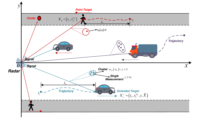
Figure 2: This figure shows a scenario consisting of both point and extended targets. For a given radar resolutions, pedestrians can be considered as point targets and vehicles as extended targets (as in the experimental results section). The measurements of each potential target form a cluster. The point target will generate at most one measurement and the extended target will generate a time-varying number of measurements within a certain range and angular spread per time step.

III-A The Coexisting Space Model

A common scenario for coexisting extended and point target is a traffic monitoring situation, as illustrated in Fig. 2. To track both kinds of targets, it is important to define a general space model. First, for the scenario in Fig. 2, we define the state of point target trajectory at time $k$ with the notation:

$${X_{p}}=(t,x_{p}^{1:i}),$$ (13)

where $t$ represents its birth time and $x_{p}^{1:i}=(x_{p}^{1},...,x_{p}^{i})$ denotes a sequence including the point target states at each time step of the trajectory with length $i$ [23]. The state $X_{p}$ belongs to the space $\mathbb{T}_{p,k}$, which is written as

$${X_{p}}\in\mathbb{T}_{p,k}=\uplus_{(t,i)\in\mathbb{I}_{k}}\{t\}\times\mathbb{R}^{i\times n_{x}},$$ (14)

To describe an extended target state $X^{+}_{e}$ at time $k$, we respectively define the notation $X_{e}$ for trajectory state, $\gamma$ for the expected number of measurements per target and $\tilde{X}$ for the extent state[28]. More specifically,

$$X^{+}_{e}=(X_{e},\gamma,\tilde{X})\in \mathbb{T}_{e,k},$$ (15)

$$X_{e}=(t,x^{1:i}_{e})\in \uplus_{(t,i)\in\mathbb{I}_{k}}\{t\}\times\mathbb{R}^{i\times n_{x}},$$ (16)

$$\gamma\in \mathbb{R}_{+},$$ (17)

$$\tilde{X}\in \mathbb{S}^{d}_{+},$$ (18)

where $x_{e}^{1:i}$ denotes the sequence of target states, $\mathbb{R}_{+}$ represents the space of positive real numbers and $\mathbb{S}^{d}_{+}$ is the space of positive definite matrices with size $d$. The value of $d$ is taken as the dimension of the target extent. Here, we only consider target extent $\tilde{X}$ and $\gamma$ at the latest time step for simplicity. If the historical information needs to be stored, we just add the corresponding sequence to the trajectory space. Therefore, the coexisting trajectory space for both point and extended targets is given as $\mathbb{T}_{k}=\mathbb{T}_{p,k}\uplus\mathbb{T}_{e,k}$.

III-B The GGIW Model

The implementation is provided for a Gaussian model for point target trajectory [40, 18, 23] and a Gamma Gaussian Inverse Wishart (GGIW) model for extended target trajectory. [32, 33, 28, 34].

The density of $\gamma$ is given as the Gamma distribution ${\cal G}(\gamma;a,b)$ with parameters $a>0$ and $b>0$. The Inverse Wishart density on matrices ${\cal{IW}}(\tilde{X};v,V)$ is used to describe $\tilde{X}$, which is defined in space $\mathbb{S}^{d}_{+}$ with $v>2d$ degrees of freedom and parameter matrix $V\in\mathbb{S}^{d}_{+}$. The Gamma and Inverse Wishart distributions are known as the conjugate prior to the Poisson distribution and multivariate Gaussian distribution, respectively. The derivation of these two distributions in Bayesian recursion can be found in [42, 43].

At time $k$, the Gaussian density of the trajectory $X=(t,x^{1:i})$ is denoted as [23]

$${\cal N}({X;t^{k},\widehat{m}^{k},\widehat{P}^{k}})={\cal N}({x^{1:i};\widehat{m}^{k},\widehat{P}^{k}})\delta_{[t^{k}]}[t]\delta_{[i^{k}]}[i].$$ (19)

where $\widehat{m}^{k}\in\mathbb{R}^{i{n_{x}}}$ and $\widehat{P}^{k}\in\mathbb{R}^{i{n_{x}}\times i{n_{x}}}$ denote the mean and covariance, respectively. The term $t^{k}=k-i^{k}+1$ denotes the trajectory birth time and $i^{k}=\text{dim}(\widehat{m}^{k}/n_{x})$.

Then, to calculate the PHD $\lambda_{k|k}(X)$ at time $k$, we have that

$$\lambda_{k|k}(X)=\lambda_{k|k}^{e}(X)+\lambda_{k|k}^{p}(X),$$ (20)

where $\lambda_{k|k}^{e}(X)=0$ if $X\in\mathbb{T}_{p,k}$ and $\lambda_{k|k}^{p}(X)=0$ if $X\in\mathbb{T}_{e,k}$. Therefore, we can write the two terms at the right side of the above equation as

$${\lambda^{e}_{k|k}}\left(X^{+}_{e}\right)= \sum\limits_{j=1}^{{J_{e}^{k|k}}}\omega_{e,j}^{k|k}{\cal G}\left({\gamma;a_{j}^{k|k},b_{j}^{k|k}}\right)$$

$$\times{\cal N}\left({X_{e};t_{e,j},\widehat{m}_{e,j}^{k|k},\widehat{P}_{e,j}^{k|k}}\right)$$

$$\times{\cal{IW}}\left({\tilde{X};v_{j}^{k|k},V_{j}^{k|k}}\right),$$ (21)

$${\lambda^{p}_{k|k}}\left(X_{p}\right)= \sum\limits_{i=1}^{{J_{p}^{k|k}}}\omega_{p,i}^{k|k}{\cal N}\left({X_{p};t_{p,i},\widehat{m}_{p,i}^{k|k},\widehat{P}_{p,i}^{k|k}}\right),$$ (22)

where $J_{e}^{k|k},J_{p}^{k|k}$ denote the number of GGIW and Gaussian components. The notations $w_{e,j}^{k|k},w_{p,i}^{k|k}$ denote the weight for each GGIW and Gaussian component.

The dynamic model for point targets is the linear Gaussian model. That is $g(x_{p}^{i}|x_{p}^{i-1})={\cal N}(x_{p}^{i};Fx_{p}^{i-1},Q)$, where $F$ is the transition matrix and $Q$ is the process noise covariance matrix. For extended targets, the dynamic model is provided for $\gamma$, $x_{e}$ and $\tilde{X}$. There are several dynamic models [28, 44, 33]. In this paper, we use the one in [33], but the transition of target state $x_{e}$ is given as the linear Gaussian model for simplicity, i.e., $g(x_{e}^{i}|x_{e}^{i-1})={\cal N}(x_{e}^{i};Fx_{e}^{i-1},Q)$. Besides, the surviving probability is constant in implementation, i.e., $p^{S}(x)=p^{S}$. We also assume that a point target cannot become an extended target and vice versa. The $\gamma$ is assuming as a constant in the implementation.

To distinguish the measurement density $f(\mathbf{z}_{k}|\cdot)$ in eq. (5), here we use the notation $l(z|\cdot)$ to denote the single measurement model, where $z\in\mathbf{z}_{k}$ denotes a single measurement. The measurement model depends on the type of target we observe. For point targets, it is written as $l(z|x^{i})={\cal N}(z;Hx_{p}^{i},R)$, where $H$ is the observation matrix and $R$ is the noise covariance matrix. For extended targets, it is written as $l(z|x^{i})={\cal N}(z;Hx_{e}^{i},X)$. Besides, the detection probability is constant, i.e., $p^{D}(x)=p^{D}$. The relationship between $l(z|\cdot)$ and $f(\mathbf{z}|\cdot)$ for point and extended targets are given by subsections A and B in Appendix B.

For simplicity in following calculations, we define that, for a matrix $V$, the notation ${V_{\left[{n:m,s:t}\right]}}$ represents the submatrix of $V$ for rows from time steps $n$ to $m$ and columns from time steps $s$ to $t$. The notation $V_{[n:m]}$ is used to present the submatrix of $V$ for rows from time steps $n$ to $m$.

III-C Update

Proposition 3.

Given the prior PHD $\lambda_{k|k-1}(\cdot)$ of the form (20) and the measurement set $\mathbf{z}_{k}$, the posterior PHD $\lambda_{k|k}(\cdot)$ is

$${\lambda_{k|k}}\left(X\right)={\lambda_{k|k}^{ND}}\left(X\right)+\sum_{\mathcal{P}\angle\mathbf{z}_{k}}\sum_{\mathbf{w}\in\mathcal{P}}{\lambda_{k|k}^{D}}\left(X,\mathbf{w}\right).$$ (23)

Following eq. (20), the mis-detected part ${\lambda_{k|k}^{ND}}\left(X\right)$ can be written as the sum of $\lambda_{k|k}^{e,ND}(X)$ and $\lambda_{k|k}^{p,ND}(X)$, which is respectively given as

$${\lambda_{k|k}^{e,ND}}\left(X^{+}_{e}\right)= \sum\limits_{j=1}^{{J_{e}^{k|k-1}}}\omega_{e,j}^{k|k-1}{\cal N}\left({X_{e};t_{e,j},\widehat{m}_{e,j}^{k|k-1},\widehat{P}_{e,j}^{k|k-1}}\right)$$

$$\times{\cal{IW}}\left({\tilde{X};v_{j}^{k|k-1},V_{j}^{k|k-1}}\right)$$

$$\times\left[(1-p^{D}){\cal G}\left({\gamma;a_{j}^{k|k-1},b_{j}^{k|k-1}}\right)\right.$$

$$\left.+p^{D}\left(\frac{b_{j}^{k|k-1}}{b_{j}^{k|k-1}+1}\right)^{a_{j}^{k|k-1}}\right.$$

$$\left.\times{\cal G}\left({\gamma;a_{j}^{k|k-1},b_{j}^{k|k-1}+1}\right)\right],$$ (24)

$${\lambda_{k|k}^{p,ND}}\left(X_{p}\right)= \sum\limits_{i=1}^{{J_{p}^{k|k-1}}}(1-p^{D})\omega_{p,i}^{k|k-1}$$

$$\times{\cal N}\left({X_{p};t_{p,i},\widehat{m}_{p,i}^{k|k-1},\widehat{P}_{p,i}^{k|k-1}}\right).$$ (25)

For extended targets, the update of mis-detected part has two ways. The first corresponds to the situation of the missed detection, which is modeled by $p^{D}$. The second corresponds to the situation that the Poisson random number of detections is zero, also governed by the factors $a,b$ of Gamma density [33, 42]. While for point targets, the update of that only concerns the missed detection situation [18, 23]. Conversely, the detected part ${\lambda_{k|k}^{D}}(X,\mathbf{w})$ can be decomposed as

$${\lambda_{k|k}^{e,D}}\left(X^{+}_{e},\mathbf{w}\right)= \sum\limits_{j=1}^{{J_{e}^{k|k-1}}}\omega_{e,j}^{k}(\mathbf{w}){\cal G}\left({\gamma;a_{j}^{k},b_{j}^{k}}\right)$$ (26)

$$\times {\cal N}\left({X_{e};t_{e,j},\widehat{m}_{e,j}^{k},\widehat{P}_{e,j}^{k}}\right){\cal{IW}}\left({\tilde{X};v_{j}^{k},V_{j}^{k}}\right),$$

$${\lambda_{k|k}^{p,D}}\left(X_{p},\mathbf{w}\right)= \sum\limits_{i=1}^{{J_{p}^{k|k-1}}}\omega_{p,i}^{k}(\mathbf{w}){\cal N}\left({X_{p};t_{p,i},\widehat{m}_{p,i}^{k},\widehat{P}_{p,i}^{k}}\right),$$ (27)

where

$$\omega_{e,j}^{k}(\mathbf{w})= \frac{\omega_{\mathcal{P}}}{d_{\mathbf{w}}}\omega_{e,j}^{k|k-1}p^{D}\frac{q_{e,j}(\mathbf{w})}{\left[\lambda^{C}\left(\cdot\right)\right]^{\mathbf{w}}}q_{e,j}(\mathbf{w}),$$ (28)

$$\omega_{p,i}^{k}(\mathbf{w})= \frac{\omega_{\mathcal{P}}}{d_{\mathbf{w}}}\omega_{p,i}^{k|k-1}p^{D}\cdot\frac{q_{p,i}(\mathbf{w})}{\lambda^{C}\left(\cdot\right)}\delta_{1}[|\mathbf{w}|],$$ (29)

$$\omega_{\mathcal{P}}= \frac{\prod_{\mathbf{w}\in\mathcal{P}}d_{\mathbf{w}}}{\sum_{\mathcal{Q}\angle\mathbf{z}_{k}}\prod_{\mathbf{w}\in\mathcal{Q}}d_{\mathbf{w}}},$$ (30)

$$d_{\mathbf{w}}= \delta_{1}[|\mathbf{w}|]+\sum\limits_{l=1}^{{J_{e}^{k|k-1}}}\omega_{e,l}^{k|k-1}p^{D}\frac{q_{e,l}(\mathbf{w})}{\left[\lambda^{C}\left(\cdot\right)\right]^{\mathbf{w}}}$$

$$+\sum\limits_{o=1}^{{J_{p}^{k|k-1}}}{\omega_{p,o}^{k|k-1}p^{D}\frac{q_{p,o}(\mathbf{w})}{\lambda^{C}\left(\cdot\right)}\delta_{1}[|\mathbf{w}|]}.$$ (31)

It is worth noting that if $|\mathbf{w}|>1$, the target must be an extended target, but if $|\mathbf{w}|=1$, the target may be a point, an extended target or the clutter. Therefore, we add the delta function $\delta_{1}[|\mathbf{w}|]$ in eqs. (29) and (31). For the specific update for the factors of GGIW components in (26), we have following equations:

$$(\widehat{m}_{e,j}^{k},\widehat{P}_{e,j}^{k},a^{k}_{j},b^{k}_{j},v^{k}_{j},V^{k}_{j})$$

$$=\left\{\begin{array}[]{ll}\widehat{m}_{e,j}^{k}&=\widehat{m}_{e,j}^{k|k-1}+{K_{j}}\epsilon_{j},\\ \widehat{P}_{e,j}^{k}&=\widehat{P}_{e,j}^{k|k-1}-{K_{j}}H\widehat{P}_{{e,j},[{k,t_{j}:k}]}^{k|k-1},\\ a_{j}^{k}&=a_{j}^{k|k-1}+|\mathbf{w}|,\\ b_{j}^{k}&=b_{j}^{k|k-1}+1,\\ v_{j}^{k}&=v_{j}^{k|k-1}+|\mathbf{w}|,\\ V_{j}^{k}&=V_{j}^{k|k-1}+N_{j}+Z,\\ \end{array}\right.$$ (38)

where

$${\bar{z}}= \frac{1}{|\mathbf{w}|}\sum_{z\in\mathbf{w}}z,$$ (39)

$$Z= \sum_{z\in\mathbf{w}}(z-\bar{z})(z-\bar{z})^{\top},$$ (40)

$$\tilde{X}_{j}= \frac{V_{j}^{k|k-1}}{v_{j}^{k|k-1}-2d-2},$$ (41)

$$\epsilon_{j}= \bar{z}-{H}\widehat{m}_{{e,j},[k]}^{k|k-1},$$ (42)

$${S_{j}}= {H}\widehat{P}^{k|k-1}_{{e,j},[k,k]}H^{\top}+\frac{\tilde{X}_{j}}{|\mathbf{w}|},$$ (43)

$${K_{j}}= \widehat{P}_{{e,j},[{t_{j}:k,k}]}^{k|k-1}H^{\top}S_{j}^{-1},$$ (44)

$$N_{j}= \tilde{X}_{j}^{{1}/{2}}S_{j}^{-1/{2}}\epsilon_{j}\epsilon_{j}^{\top}S_{j}^{-{\top}/{2}}\tilde{X}_{j}^{\top/2}.$$ (45)

To calculate the direct Gaussian update for point targets, i.e., $(\widehat{m}_{p,j}^{k},\widehat{P}_{p,j}^{k})$, we follow the same principles as [23]. Besides, the measurement likelihood function for coexisting point and extended targets is obtained by:

$${q_{p,j}}\left(\mathbf{w}\right)= {\cal N}\left({\mathbf{w};{H}\widehat{m}_{{p,j},[k]}^{k|k-1},{H}\widehat{P}^{k|k-1}_{{p,j},[k,k]}H^{\top}+R}\right),$$ (46)

$${q_{e,j}}\left(\mathbf{w}\right)= \left(\pi^{|\mathbf{w}|}|\mathbf{w}|\right)^{-d/2}\frac{\left|V_{j}^{k|k-1}\right|^{\frac{v_{j}^{k|k-1}-d-1}{2}}}{\left|V_{j}^{k}\right|^{\frac{v_{j}^{k}-d-1}{2}}}$$ (47)

$$\times\frac{\Gamma_{d}\left(\frac{v_{j}^{k}-d-1}{2}\right)\left|\tilde{X}_{j}\right|^{1/2}\Gamma(a_{j}^{k})(b_{j}^{k|k-1})^{a_{j}^{k|k-1}}}{\Gamma_{d}\left(\frac{v_{j}^{k|k-1}-d-1}{2}\right)|S_{j}|^{1/2}\Gamma(a_{j}^{k|k-1})(b_{j}^{k})^{a_{j}^{k}}},$$

where $\Gamma$ is the Gamma function and $\Gamma_{d}$ is the multivariate Gamma function. Then, we complete the process of update step in general TPHD filter using GGIW mixture.

III-D Prediction

The PHD of the birth density is given as

$${\lambda_{\gamma,k|k}}\left(X\right)={\lambda^{e}_{\gamma,k|k}}\left(X\right)+{\lambda^{p}_{\gamma,k|k}}\left(X\right)$$ (48)

where

$${\lambda^{e}_{\gamma,k|k}}\left(X^{+}_{e}\right)= \sum\limits_{j=1}^{J_{\gamma^{e}}^{k}}{\omega_{\gamma^{e},j}^{k}{\cal G}\left({\gamma;a_{\gamma,j}^{k},b_{\gamma,j}^{k}}\right)}$$ (49)

$$\times{{\cal N}\left({X_{e};k,\widehat{m}_{\gamma^{e},j}^{k},\widehat{P}_{\gamma^{e},j}^{k}}\right)}$$

$$\times{\cal{IW}}\left({\tilde{X};v_{\gamma,j}^{k},V_{\gamma,j}^{k}}\right),$$

$${\lambda^{p}_{\gamma,k|k}}\left(X_{p}\right)= \sum\limits_{i=1}^{{J_{\gamma^{p}}^{k}}}\omega_{\gamma^{p},i}^{k}{{\cal N}\left({X_{p};k,\widehat{m}_{\gamma^{p},i}^{k},\widehat{P}_{\gamma^{p},i}^{k}}\right)}.$$ (50)

The notations $J_{\gamma^{e}}^{k}$ and $J_{\gamma^{p}}^{k}$ denote the number of PHD components for new born targets. For the $j$-th birth component at time $k$, $\omega_{\gamma^{e},j}^{k}$ and $\omega_{\gamma^{e},j}^{k}$ represent the weight of extended and point target, respectively.

Proposition 4.

Given the posterior PHD $\lambda_{k-1|k-1}(\cdot)$ for coexisting point and extended trajectory at time $k-1$, the prior PHD $\lambda_{k|k-1}(\cdot)$ is

$${\lambda_{k|k-1}}\left(X\right)= \lambda_{\gamma,k|k}\left(X\right)+\lambda^{S}_{k|k-1}\left(X\right),$$ (51)

$$\lambda^{S}_{k|k-1}\left(X\right)= \lambda^{S,e}_{k|k-1}\left(X\right)+\lambda^{S,p}_{k|k-1}\left(X\right),$$ (52)

where

$${\lambda^{S,e}_{k|k-1}}\left(X^{+}_{e}\right)= {p^{S}}\sum\limits_{j=1}^{{J_{e}^{k-1}}}{\omega_{e,j}^{k-1}{\cal G}\left({\gamma;a_{S,j}^{k|k-1},b_{S,j}^{k|k-1}}\right)}$$

$$\times{{\cal N}\left({X_{e};t_{e,j},\widehat{m}_{S^{e},j}^{k|k-1},\widehat{P}_{S^{e},j}^{k|k-1}}\right)}$$

$$\times{\cal{IW}}\left({\tilde{X};v_{S,j}^{k|k-1},V_{S,j}^{k|k-1}}\right),$$ (53)

$${\lambda^{S,p}_{k|k-1}}\left(X_{p}\right)= p^{S}\sum\limits_{i=1}^{{J_{p}^{k-1}}}\omega_{p,i}^{k-1}{{\cal N}\left({X_{p};t_{p,i},\widehat{m}_{S^{p},i}^{k|k-1},\widehat{P}_{S^{p},i}^{k|k-1}}\right)}.$$ (54)

The Gaussian components of both point and extended target trajectory share the same prediction equations, so here for both $u=p$ and $u=e$, we have that:

$$\widehat{m}_{S^{u},j}^{k|k-1}= \left[{\left[\widehat{m}_{u,j}^{k-1}\right]^{\top},\left[F\cdot\widehat{m}_{{u,j},[k-1]}^{k-1}\right]^{\top}}\right]^{\top},$$ (55)

$$\widehat{P}_{S^{u},j}^{k|k-1}= \left[{\begin{array}[]{*{20}{c}}{\widehat{P}_{u,j}^{k-1}}&P_{1}\\ P_{1}^{\top}&P_{2}\end{array}}\right],$$ (58)

$$P_{1}= {\widehat{P}_{{u,j},\left[{t_{u,j}:k-1,k-1}\right]}^{k-1}{F^{\top}}},$$ (59)

$$P_{2}= {F\widehat{P}_{{u,j},[k-1,k-1]}^{k-1}F^{\top}+Q}.$$ (60)

Then, the prediction steps for the Gamma and Inverse Wishart components are given as:

$$a_{S,j}^{k|k-1}= a_{j}^{k-1}/\mu,$$ (61)

$$b_{S,j}^{k|k-1}= b_{j}^{k-1}/\mu,$$ (62)

$$v_{S,j}^{k|k-1}= 2d+2+e^{-\delta_{t}/\tau}(v_{j}^{k-1}-2d-2),$$ (63)

$$V_{S,j}^{k|k-1}= e^{-\delta_{t}/\tau}M(\widehat{m}_{{e,j},[k-1]}^{k-1})V_{j}^{k-1}M^{\top}(\widehat{m}_{{e,j},[k-1]}^{k-1}),$$ (64)

where $\mu$ denotes the measurement rate parameter, $\delta_{t}$ is the sampling time period, $\tau$ is the correlation constant and $M(\cdot)$ is the transformation matrix for extent model [33].

III-E Strategies to Lower the Computational Cost

In this subsection, we introduce two strategies to make filter implementation tractable.

To restrict the unbounded increasing GGIW and Gaussian components, we can adopt the pruning and absorption techniques [23].

TABLE I: The Algorithm For Pruning and Absorption

Input: the posterior PHD parameters $\{\Phi_{e,j}^{k}\}_{j=1}^{J_{e}^{k}}$ for extended and $\{\Phi_{p,j}^{k}\}_{j=1}^{J_{p}^{k}}$ for point target trajectory, which are Φ_e,j^k={ω_e,j^k,t_e,j,i_e,j^k,^m_e,j^k,^P_e,j^k,a^k_j,b^k_j,v^k_j,V^k_j } and Φ_p,j^k={ω_p,j^k,t_p,j,i_p,j^k,^m_p,j^k,^P_p,j^k }, and the pruning threshold $\mathit{\Gamma_{p}}$, absorption threshold $\mathit{\Gamma_{a}}$ and maximum allowable number of components $J_{max}$.

For $u=e$ or $p$:

Set $\ell=0$ and $\Theta=\left\{i=1,...,J_{u}^{k}|\omega_{u,i}^{k}>\mathit{\Gamma_{p}}\right\}$.

Loop

$\ell=\ell+1.$ $j$ = $arg$$\mathop{max}\limits_{i\in\Theta}$ $\omega_{u,i}^{k}$. $L=\{i\in\Theta:(\widehat{m}_{{u,i},[k]}^{k}-\widehat{m}_{{u,j},[k]}^{k})^{\top}(\widehat{P}_{{u,j},[k,k]}^{k})^{-1}(\widehat{m}_{{u,i},[k]}^{k}-\widehat{m}_{{u,j},[k]}^{k})\leq\mathit{\Gamma_{a}}\}$. $\bar{\omega}_{\ell}^{k}=\sum\nolimits_{i\in L}\omega_{u,i}^{k}$, $\bar{\Phi}_{\ell}^{k}=\Phi_{u,j}^{k}$ with weight $\bar{\omega}_{\ell}^{k}$. $\Theta=\Theta\backslash L$.

If $\Theta=\emptyset$, break

if $\ell>J_{max}$ then replace $\bar{\Phi}_{\ell}^{k}$ by the $J_{max}$ components with largest weights.

Output:$\{\bar{\Phi}_{j}^{k}\}_{j=1}^{min\{\ell,J_{max}\}}$.

The pruning step aims at deleting the components with low weights and absorption step is to restrict the maximum number of components as well as only retaining the component with higher weight for two closely spaced GGIW/Gaussian components. The process is given in the Table I.

To limit the increasing computational cost of handling trajectories with increasing lengths, the $L$-scan approximation [23] is applied, which only updates the density of the last $L$ time and leaves the rest unaltered. The further information about the $L$-scan approximation can be found in [23]. In this paper, the implementation of the PHD filter for coexisting point and extended targets can be obtained by taking the last time step estimates of the general TPHD filters, i.e., the value of $L$-scan is taken as 1[23].

IV Numerical Results

In this section, we compare the general TPHD filter (G-TPHD) for coexisting extended and point target with the TPHD filter for point targets (P-TPHD) [23], the TPHD filter for extended targets (E-TPHD) [36] and the developed PHD filter (G-PHD) for coexisting situation.

IV-A Simulation Scenario

This simulation aims at showing a brief traffic environment with the size of $[{{\rm{-25}},{\rm{25}}}]\text{m}\times[{{\rm{0}},{\rm{300}}}]\text{m}$, where two extended targets and three point target are moving during 100 seconds (Table II). The target state matrix is given as $x={[{{p_{x}},{p_{y}},{{\dot{p}}_{x}},{{\dot{p}}_{y}}}]^{\top}}$ including the position (with unit: $m$) and velocity information (with unit: $m/s$). The observation matrix $z={[{{z_{x}},{z_{y}}}]^{\top}}$ includes the position information. The single target transition model is given as

$$F= \left[{\begin{array}[]{*{20}{c}}{{I_{2}}}&{{I_{2}}\delta t}\\ {{0_{2}}}&{{I_{2}}}\end{array}}\right]\qquad Q=\sigma_{v}^{2}\left[{\begin{array}[]{*{20}{c}}{\frac{{\delta{t^{4}}}}{4}{I_{2}}}&{\frac{{\delta{t^{3}}}}{2}{I_{2}}}\\ {\frac{{\delta{t^{3}}}}{2}{I_{2}}}&{\delta{t^{2}}{I_{2}}}\end{array}}\right]$$

$$H= \left[{\begin{array}[]{*{20}{c}}{{I_{2}}}&{{0_{2}}}\end{array}}\right]\qquad\leavevmode\nobreak\ \leavevmode\nobreak\ \leavevmode\nobreak\ R=\sigma_{\varepsilon}^{2}{I_{2}}$$

where ${I_{2}}$ represents the $2\times 2$ unit matrix, $0_{2}$ represents the $2\times 2$ zero matrix, $\sigma_{v}^{2}=0.1m{s^{-2}}$, $\sigma_{\varepsilon}^{2}=1m{s^{-2}}$. The notation $\delta t=1s$ denotes the sampling period.

TABLE II: The Simulated Target States

	Kind	Kinematic State	Birth Time$/s$	Death Time$/s$
Target 1	Extended	$\left[6,50,0,2\right]^{\top}$	1	100
Target 2	Point	$\left[13,48,0,2.2\right]^{\top}$	7	100
Target 3	Point	$\left[9.5,30,0,2.5\right]^{\top}$	10	80
Target 4	Extended	$\left[-7,300,0,-5.4\right]^{\top}$	20	70
Target 5	Point	$\left[-12,220,0,-1\right]^{\top}$	25	100

TABLE III: Filter Parameters

G-TPHD filter		Value
Surviving probability	$p^{S}$	0.99
Detection probability	$p^{D}$	0.98
Mean number of clutter/per scan	$\lambda_{c}$	5
Threshold of pruning	$\mathit{\Gamma_{p}}$	$10^{-5}$
Threshold of absorption	$\mathit{\Gamma_{a}}$	$4$
Maximum components	$J_{max}$	$100$
Value of $L$-scan	$L$	$5$
Dimension of $\mathbb{S}_{+}^{d}$	$d$	2
Birth weight of target	$[\omega_{\gamma^{e}},\omega_{\gamma^{p}}]$	$0.1\times[0.5,0.5]$
Birth parameters of Gamma	$a,b$	$8,1$
Birth parameters of Inverse Wishart	$v,V$	$100,2.5I_{d}$
Measurement rate(eq. (61))	$\mu$	$1.05$
Correlation constant(eq. (63))	$\tau$	$5.48$
Transformation matrix(eq. (64))	$M(\cdot)$	$I_{d}$
Parameters of DBSCAN	$\tau_{db},\Gamma_{min},\Gamma_{max}$	$0.1,0.1,8$

The parameters in our proposed G-TPHD filter are given in Table III. For simulated extended targets, we set the mean number of generated measurements per scan is 10 and the size of target extent is no more than the width of lane (3.5m).

For measurement clustering, we generate possible partitions $\mathcal{P}$ of measurement set $\mathbf{z}$ by using the DBSCAN algorithm [45] with distance thresholds between $\Gamma_{min}$ and $\Gamma_{max}$, with a step size of $\tau_{db}$ (unit: $m$). The minimum number of points to form a region is set to 1 to capture point target measurements. Meanwhile, we only keep the unique partitions among all possible generated partition and we obtain the unique subsets of measurements in these partitions.

Besides, the number of clutter measurements per scan is Poisson distributed and the clutter location is uniformly distributed in region $[-25,25]$m$\times$$[0,300]$m. In this paper, we use the root mean square (RMS) trajectory metric (TM) error[46] to evaluate the performance of proposed filter. The relevant parameters of RMS TM error is given as $p=2,c=100,\gamma=1$.

Figure 3: This figure shows a simulated traffic environment, where five different targets are moving within 100s. The radar sensor is set at the position $(0,0)$. The start and end points for each true trajectory are marked by o and $*$, respectively. The black lines denote the true trajectories for all targets during the whole time period (100s). We present the estimated target trajectories (purple lines) and extent model of the targets at the time step 67s. The true extent for “Targets 1 and 4” and their estimates are marked through blue and red lines, respectively.

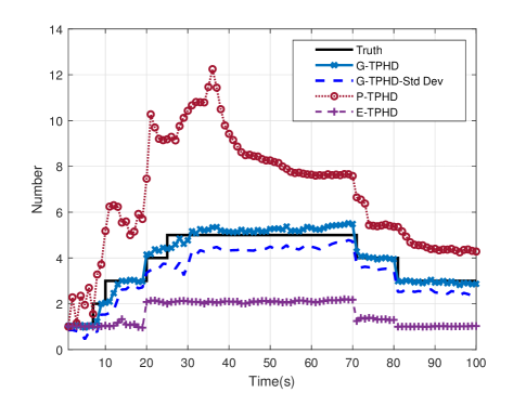
Figure 4: This figure shows the number estimates of alive trajectories over the G-TPHD, E-TPHD and P-TPHD filters. All estimates are averaged by 500 Monte Carlo runs.

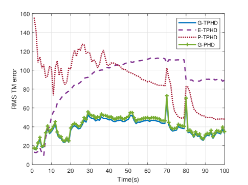
Figure 5: The figure shows the RMS TM error for the G-TPHD filter as well as the E-TPHD, P-TPHD and G-PHD filters.

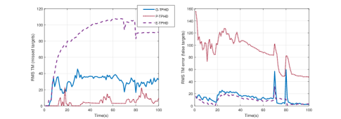
Figure 6: The figure shows the decomposition of the RMS TM error for false and missed targets.

TABLE IV: The RMS TM Error and Its Decomposition (Normalized by Time Window)

	Mean	Localization	Miss	False	Switch
G-TPHD	38.79	4.95	31.21	21.20	0.025
G-PHD	40.65	5.28	32.31	22.56	0.029
P-TPHD	89.20	1.89	4.94	88.92	0.096
E-TPHD	87.58	4.56	85.91	9.20	0.031

It can be seen from Fig. 3 that the proposed filter can track point and extended targets at the same time, and output their current position and trajectory information. From Table IV and Figs. 4 – 6, the G-TPHD filter is more accurate in estimating the target trajectory and the number of targets at each time step compared to the E-TPHD, P-TPHD and G-PHD filters.

For the advantages of the proposed G-TPHD filter over the G-PHD filter in Fig. 5, the former considers using current measurements to update the whole trajectory so that a better estimate can be obtained. The G-PHD filter is taken as a simplified version of the G-TPHD filter, which can be obtained by setting the value of $L$-scan equals as 1.

For the comparisons of the G-TPHD, E-TPHD and P-TPHD filters in Figs. 4 – 6. It is manifest that the tracking performance of the proposed filter is much better than other two counterparts. The reason is explained in Fig. 6, which shows the error for false alarm targets and missed targets. For the P-TPHD filter that only considers point target tracking, extended targets with multiple measurements will cause more false target estimates. On the other hand, for the E-TPHD filter that only considers extended target tracking, the hypothesis of point target has a smaller posterior probability due to the lack of support in likelihood function, resulting in more missed target errors. For the proposed G-TPHD filter, we have more robust performance because we consider the coexistence space of point targets and extended targets and a general measurement likelihood function, which provides a better support for hypotheses of both extended and point targets.

IV-B Experimental Scenario

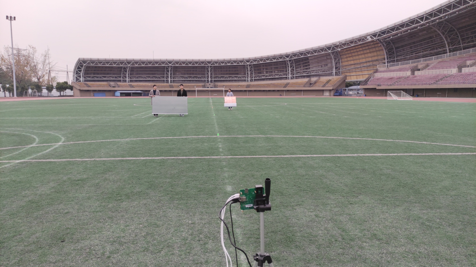
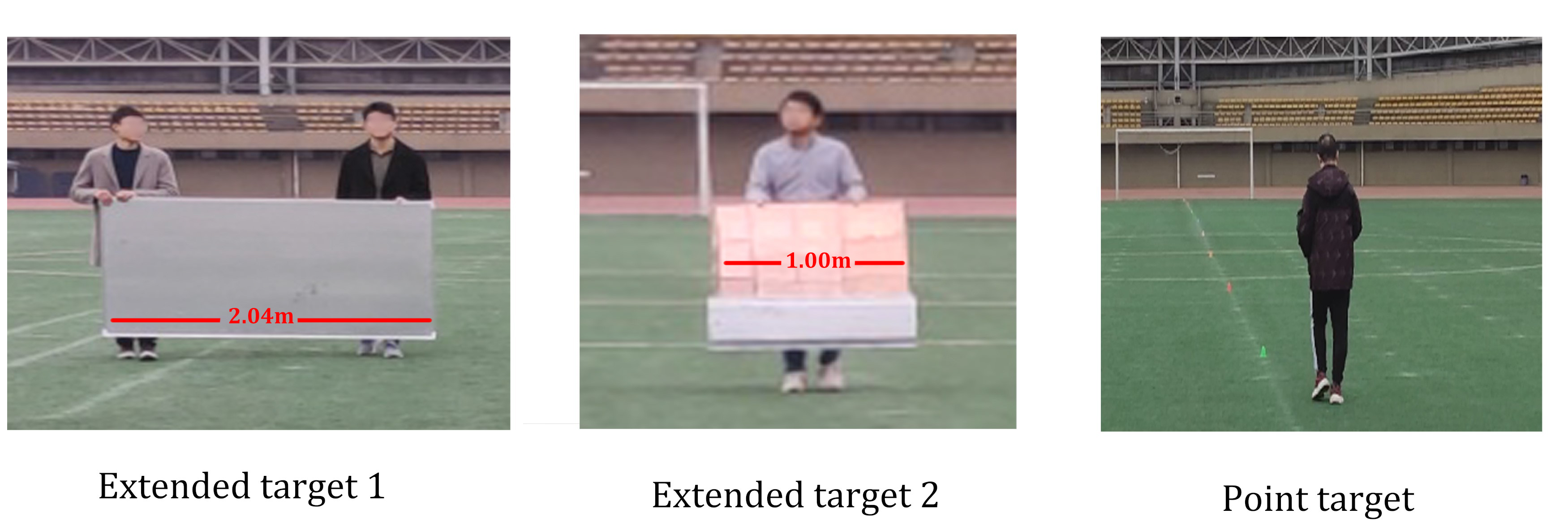
In this subsection, we present the signal processing and tracking results from the measured radar data. The experimental scenario is from the playground of the university campus, as shown in Fig. 7. There are two extended targets and two point targets. Both of them move in an approximately straight line. The extended targets consist of people and a metal board, while the point target is a single person, as shown in Fig. 8. The transmitting signal is frequency modulated continuous wave (FMCW) with the start frequency 77GHz. The Bandwidth is set as 800MHz. The number of chirp loops and ADC samples are 128 and 256, respectively. The structure of the radar equipment consists of 1 transmitting antenna and 4 receiving antennas. The total length of the data used in tracking is 7s (70 frames) and the filter parameters are the same with those in Subsection A.

Figure 7: The experimental scenario.

Figure 8: The targets in the tracking scenario (two kinds of extended target with different size and two point targets).

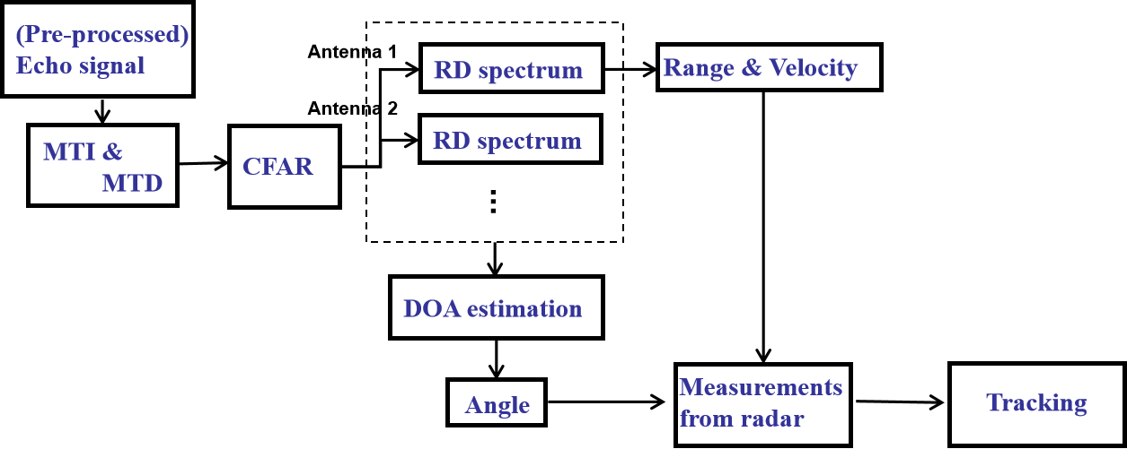
Figure 9: The signal processing flow for collected data from Fig 7.

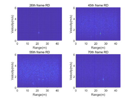
Figure 10: The figure shows the range and Doppler (RD) spectrum of one radar channel at the 20th, 45th, 55th and 70th frames. A brighter color represents a stronger signal.

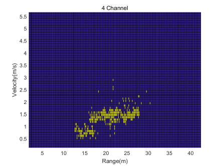
Figure 11: It shows the result after CFAR, which sums over 4 channels of radar RD spectrum during the whole tracking period (70 frames). Here, the amplitude of all selected peaks after CFAR is set as 1.

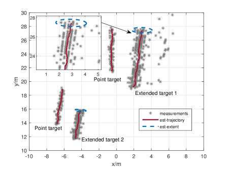
Figure 12: Two point and two extended targets are moving away from the radar at the origin during the time period from the 1st frame to the 70th frame. The tracking results are represented with red lines and the estimates of the target extent are represented with blue dotted lines. Asterisks represent measurements.

The signal processing steps are given by the flow chart Fig. 9. The Moving Target Indicator (MTI) filter is achieved by the transfer function $H(z)=1-z^{-1}$ to eliminate the static target and clutter. The Doppler and range information is obtained by doing fast Fourier transform (FFT) for the slow and fast time dimension respectively. After obtaining the range and Doppler (RD) spectrum, we use the constant-false-alarm-rate (CFAR) technique to extract peaks by setting the threshold. Here, we adopted a square and two-dimensional Cell-Averaging-CFAR (CA-CFAR) [47]. The constant false alarm rate is set as $P_{fa}=1\times 10^{-6}$, the number of protection units is $N_{p}=48$, and the number of reference units is $N_{r}=312$. The RD spectrum and its result after CFAR are given in Figs. 10 and 11. To get the angular information, we do FFT directly on the angel dimension. Then by combining the distance information after CFAR and angel information, we can obtain the X-Y position information of targets and use it as the measurement set for the proposed filter to track. The estimated trajectory result is shown in Fig. 12. It can be seen that our proposed filter can distinguish point target and extended target well. Besides, based on the ellipse model for target extent, we can make the average estimates for the widths of two extended targets, which are shown in Table V.

TABLE V: Estimated Width for the Extended Targets

Category	True Width (m)	Estimated Width (m)
Extended Target 1	2.04	2.24
Extended Target 2	1.00	1.25

V Conclusion

In this paper, we have derived a TPHD filter for general target-generated measurements by approximating the posterior density by a Poisson density using direct KLD minimization without using PGFLs. The proposed TPHD filter is able to output the trajectory estimates of both point and extended targets simultaneously. In addition, we have proposed an implementation of this filter based on a Gamma Gaussian Inverse Wishart mixture model. Considering the tracking efficiency, a $L$-scan approximate version is proposed to reduce the computational cost. Finally, the simulation and experimental results proved that the proposed TPHD filter has a robust performance in coexisting point and extended target scenarios.

Appendix A

We aim to prove Proposition 1 by finding the Poisson density that best fits the posterior by minimizing the KLD, similar to the approaches in [23, 20]. We commence by writing the predicted PHD for targets as

$$\lambda_{k|k-1}\left(x\right) =\overline{\lambda}_{k|k-1}\breve{\lambda}_{k|k-1}\left(x\right),$$ (65)

where

$$\overline{\lambda}_{k|k-1} =\int\lambda_{k|k-1}\left(x\right)dx,$$ (66)

$$\breve{\lambda}_{k|k-1}\left(x\right) =\frac{\lambda_{k|k-1}\left(x\right)}{\overline{\lambda}_{k|k-1}}.$$ (67)

The notation $\overline{\lambda}$ indicates the expected number of targets. Considering the target trajectory, its corresponding PHD $\lambda_{k|k-1}\left(X\right)$ possesses the similar decomposition and the same expected number as the targets (as the PHD only considers alive trajectories). That is,

$$\int\lambda_{k|k-1}\left(x\right)dx=\int\lambda_{k|k-1}\left(X\right)dX.$$ (68)

Given the PHD $\lambda_{k|k-1}\left(X\right)$, the corresponding PPP density is

$$f_{k|k-1}\left(\left\{X_{1},...,X_{n}\right\}\right) =e^{-\overline{\lambda}_{k|k-1}}\overline{\lambda}_{k|k-1}^{n}\prod_{j=1}^{n}\breve{\lambda}_{k|k-1}\left(X_{j}\right),$$ (69)

which can be also applied in the PHD of targets $f_{k|k-1}\left(\left\{x_{1},...,x_{n}\right\}\right)$ by only changing the notation $X$ to $x$.

A-A Preliminary lemmas

The proof of the general TPHD filter update makes use of the following lemmas.

Lemma 1.

Given a set $\mathbf{z}$, and a partition $Q$ of $\mathbf{z}$ and real-valued functions $\lambda\left(\cdot\right)$ and $\tau\left(\cdot\right)$ such that

$$\lambda^{\mathbf{z}} =\begin{cases}\prod_{z\in\mathbf{z}}\lambda\left(z\right)&\mathbf{z}\neq\emptyset\\ 1&\mathbf{z}=\emptyset\end{cases}$$

$$\tau^{Q} =\begin{cases}\prod_{\mathbf{w}\in Q}\tau\left(\mathbf{w}\right)&Q\neq\emptyset\\ 1&Q=\emptyset\end{cases}$$

the following equality holds

$$\sum_{\mathbf{y}\subseteq\mathbf{z}}\lambda^{\mathbf{z}\setminus\mathbf{y}}\sum_{\mathcal{Q}\angle\mathbf{y}}\tau^{\mathcal{Q}} =\sum_{\mathcal{Q}\angle\mathbf{z}}\left(\kappa+\tau\right)^{\mathcal{Q}},$$ (70)

where $\mathbf{z}\setminus\mathbf{y}$ denotes the set difference between $\mathbf{z}$ and $\mathbf{y}$, and

$$\kappa\left(\mathbf{w}\right) =\delta_{1}\left[|\mathbf{w}|\right]\prod_{z\in\mathbf{w}}\lambda\left(z\right).$$

Lemma 1 is proved in Appendix C.

Lemma 2.

Given two real-valued functions $f\left(\cdot\right)$ and $g\left(\cdot\right)$ defined for all $\mathbf{w}\subseteq\mathbf{z}_{k}:|\mathbf{w}|>0$, the following relation holds

$$\sum_{\mathbf{w}\subseteq\mathbf{z}_{k}:|\mathbf{w}|>0}f\left(\mathbf{w}\right)\sum_{\mathcal{Q}\angle\mathbf{z}_{k}\setminus\mathbf{w}}g^{\mathcal{Q}} =\sum_{\mathcal{P}\angle\mathbf{z}_{k}}g^{\mathcal{P}}\sum_{\mathbf{v}\in\mathcal{P}}\frac{f\left(\mathbf{v}\right)}{g\left(\mathbf{v}\right)}.$$ (71)

Lemma 2 is proved in Appendix D.

A-B Density of the measurement

Given the PPP prior (69), the density of the measurement is the union of independent clutter generated measurements and target generated measurements, i.e., the density is target dependent when considering trajectory $f\left(\mathbf{z}|\left\{x_{1},...,x_{n}\right\}\right)$.

A-B1 Target-generated measurements

Applying the convolution formula, the density of the target-generated measurements given the set of targets $\mathbf{x}$ is

$$f\left(\mathbf{z}|\left\{x_{1},...,x_{n}\right\}\right) =\sum_{\mathbf{z}_{1}\uplus...\uplus\mathbf{z}_{n}=\mathbf{z}}\prod_{j=1}^{n}f\left(\mathbf{z}_{j}|x_{j}\right).$$ (72)

Then, the target-generated measurements have density

$$l_{k|k-1}^{T}\left(\mathbf{z}\right) =\int f\left(\mathbf{z}|\mathbf{x}\right)f_{k|k-1}\left(\mathbf{x}\right)\delta\mathbf{x}$$

$$=\sum_{n=0}^{\infty}\frac{1}{n!}\int\sum_{\mathbf{z}_{1}\uplus...\uplus\mathbf{z}_{n}=\mathbf{z}}\prod_{j=1}^{n}f\left(\mathbf{z}_{j}|x_{j}\right)$$

$$\quad\times e^{-\overline{\lambda}_{k|k-1}}\overline{\lambda}_{k|k-1}^{n}\prod_{j=1}^{n}\breve{\lambda}_{k|k-1}\left(x_{j}\right)dx_{1:n}$$

$$=e^{-\overline{\lambda}_{k|k-1}}\sum_{n=0}^{\infty}\frac{1}{n!}\sum_{\mathbf{z}_{1}\uplus...\uplus\mathbf{z}_{n}=\mathbf{z}}\prod_{j=1}^{n}\tau_{\mathbf{z}_{j}},$$ (73)

where $\tau_{\mathbf{w}}$ is defined in (6). We write $\mathbf{z}=\left\{z^{1},...,z^{m}\right\}$, $m>1$ then

$$l_{k|k-1}^{T} \left(\left\{z^{1},...,z^{m}\right\}\right)$$

$$= e^{-\overline{\lambda}_{k|k-1}}\sum_{n=0}^{\infty}\frac{1}{n!}\sum_{\mathbf{z}_{1}\uplus...\uplus\mathbf{z}_{n}=\left\{z^{1},...,z^{m}\right\}}\prod_{j=1}^{n}\tau_{\mathbf{z}_{j}}$$

$$= e^{-\overline{\lambda}_{k|k-1}}\sum_{n=0}^{\infty}\sum_{d=0}^{n}\frac{d!}{n!}\left(\begin{array}[]{c}n\\ d\end{array}\right)\tau_{\emptyset}^{n-d}$$ (76)

$$\times\sum_{\mathbf{z}_{1}\uplus...\uplus\mathbf{z}_{d}=\left\{z^{1},...,z^{m}\right\}:|\mathbf{z}_{{}_{i}}|\geq 1}\prod_{j=1}^{d}\tau_{\mathbf{z}_{j}}$$

$$= e^{-\overline{\lambda}_{k|k-1}}\sum_{n=0}^{\infty}\sum_{d=0}^{n}\frac{1}{\left(n-d\right)!}\tau_{\emptyset}^{n-d}\sum_{\mathcal{Q}\angle\mathbf{z}_{k}:|Q|=d}\prod_{\mathbf{w}\in\mathcal{Q}}\tau_{\mathbf{w}}$$

$$= e^{-\overline{\lambda}_{k|k-1}}\sum_{d=0}^{\infty}\sum_{\mathcal{Q}\angle\mathbf{z}_{k}:|Q|=d}\prod_{\mathbf{w}\in\mathcal{Q}}\tau_{\mathbf{w}}\sum_{j=0}^{\infty}\frac{1}{j!}\tau_{\emptyset}^{j}$$

$$= e^{-\overline{\lambda}_{k|k-1}}e^{\tau_{\emptyset}}\sum_{d=0}^{m}\sum_{\mathcal{Q}\angle\mathbf{z}_{k}:|Q|=d}\prod_{\mathbf{w}\in\mathcal{Q}}\tau_{\mathbf{w}}$$

$$= e^{-\overline{\lambda}_{k|k-1}}e^{\tau_{\emptyset}}\sum_{\mathcal{Q}\angle\mathbf{z}_{k}}\prod_{\mathbf{w}\in\mathcal{Q}}\tau_{\mathbf{w}},$$ (77)

where $d$ sums over the number of detected targets, and $j=n-d$. For $m=0$, we have

$$l_{k|k-1}^{T}\left(\emptyset\right) =e^{-\overline{\lambda}_{k|k-1}}\sum_{n=0}^{\infty}\frac{1}{n!}\tau_{\emptyset}^{n}$$ (78)

$$=e^{-\overline{\lambda}_{k|k-1}}e^{\tau_{\emptyset}}.$$

A-B2 Adding clutter

The density of the measurement is the union of independent target-generated measurements and clutter measurements. We can use the convolution formula[12] to provide

$$l_{k|k-1}\left(\mathbf{z}_{k}\right)= e^{-\overline{\lambda}^{C}}\sum_{\mathbf{z}^{T}\uplus\mathbf{z}^{C}=\mathbf{z}_{k}}l_{k|k-1}^{T}\left(\mathbf{z}^{T}\right)\prod_{z\in\mathbf{z}^{C}}\lambda^{C}\left(z\right)$$

$$= e^{-\overline{\lambda}^{C}}e^{-\overline{\lambda}_{k|k-1}}e^{\tau_{\emptyset}}\sum_{\mathbf{z}^{T}\uplus\mathbf{z}^{C}=\mathbf{z}_{k}}\sum_{\mathcal{Q}\angle\mathbf{z}^{T}}\prod_{\mathbf{w}\in\mathcal{Q}}\tau_{\mathbf{w}}$$

$$\times\prod_{z\in\mathbf{z}^{C}}\lambda^{C}\left(z\right)$$

$$= e^{-\overline{\lambda}^{C}}e^{-\overline{\lambda}_{k|k-1}}e^{\tau_{\emptyset}}\sum_{\mathbf{z}^{T}\subseteq\mathbf{z}_{k}}\sum_{\mathcal{Q}\angle\mathbf{z}^{T}}\prod_{\mathbf{w}\in\mathcal{Q}}\tau_{\mathbf{w}}$$

$$\times\prod_{z\in\mathbf{z}_{k}\setminus\mathbf{z}^{T}}\lambda^{C}\left(z\right)$$

$$= e^{-\overline{\lambda}^{C}}e^{-\overline{\lambda}_{k|k-1}}e^{\tau_{\emptyset}}\sum_{\mathcal{Q}\angle\mathbf{z}_{k}}\prod_{\mathbf{w}\in\mathcal{Q}}\left(\kappa_{\mathbf{w}}+\tau_{\mathbf{w}}\right),$$ (79)

where the notation $\overline{\lambda}^{C}$ is the expected number of clutter measurements. We have also applied the Lemma 1 in the last step.

A-C KLD minimization

The posterior is obtained as the application of Bayes’ rule (3) when the predicted density is the PPP (69)

$$f_{k|k}\left(\mathbf{X}\right) =\frac{f\left(\mathbf{z}_{k}|\mathbf{x}\right)e^{-\overline{\lambda}_{k|k-1}}\overline{\lambda}_{k|k-1}^{n}\prod_{X\in\mathbf{X}}\breve{\lambda}_{k|k-1}\left(X\right)}{l_{k|k-1}\left(\mathbf{z}_{k}\right)}.$$ (80)

The best Poisson multi-trajectory density that minimizes the KLD has the same PHD as (80) [23]. This PHD can be calculated as [12]

$$\lambda_{k|k}\left(X\right) =\int f_{k|k}\left(\left\{X\right\}\cup\mathbf{X}\right)\delta\mathbf{X}$$ (81)

$$=\sum_{n=0}^{\infty}\frac{1}{n!}\int f_{k|k}\left(\left\{X,X_{1},...,X_{n}\right\}\right)dX_{1:n}.$$

We proceed to compute (81). We first perform a decomposition of the measurement likelihood and then the PHD calculation.

A-C1 Decomposition of the likelihood

Applying the convolution formula, we can write

$$f\left(\mathbf{z}_{k}|\left\{x,x_{1},...,x_{n}\right\}\right)= \sum_{\mathbf{z}_{1}\uplus...\uplus\mathbf{z}_{n}\uplus\mathbf{w}\uplus\mathbf{z}^{C}=\mathbf{z}_{k}}f\left(\mathbf{w}|x\right)$$ (82)

$$\times e^{-\overline{\lambda}^{C}}\prod_{j=1}^{n}f\left(\mathbf{z}_{j}|x_{j}\right)\prod_{z\in\mathbf{z}^{C}}\lambda^{C}\left(z\right).$$

Expanding over the cases $\mathbf{w}=\emptyset$ and $|\mathbf{w}|>0$, we obtain

$$f \left(\mathbf{z}_{k}|\left\{x,x_{1},...,x_{n}\right\}\right)$$ (83)

$$= f\left(\emptyset|x\right)f\left(\mathbf{z}_{k}|\left\{x_{1},...,x_{n}\right\}\right)$$

$$+\sum_{\mathbf{w}\subseteq\mathbf{z}:|\mathbf{w}|>0}f\left(\mathbf{w}|x\right)f\left(\mathbf{z}_{k}\setminus\mathbf{w}|\left\{x_{1},...,x_{n}\right\}\right),$$

which can be analogously written as

$$f\left(\mathbf{z}_{k}|\left\{x\right\}\cup\mathbf{x}\right) =f\left(\emptyset|x\right)f\left(\mathbf{z}_{k}|\mathbf{x}\right)$$ (84)

$$+\sum_{\mathbf{w}\subseteq\mathbf{z}_{k}:|\mathbf{w}|>0}f\left(\mathbf{w}|x\right)f\left(\mathbf{z}_{k}\setminus\mathbf{w}|\mathbf{x}\right)$$

A-C2 PHD calculation

The PHD of the posterior is given by

$$\lambda_{k|k}\left(X\right)= \int f_{k|k}\left(X\cup\mathbf{X}\right)\delta\mathbf{X}$$

$$= \frac{\lambda_{k|k-1}\left(X\right)}{l_{k|k-1}\left(\mathbf{z}_{k}\right)}\int f\left(\mathbf{z}_{k}|\left\{x\right\}\cup\mathbf{x}\right)e^{-\overline{\lambda}_{k|k-1}}$$

$$\times\prod_{x\in\mathbf{x}}\lambda_{k|k-1}(x)\delta\mathbf{x}.$$

Substituting (84) into the above equation, we can write

$$\lambda_{k|k}\left(X\right)= f\left(\emptyset|x\right)\lambda_{k|k-1}\left(X\right)+\frac{\lambda_{k|k-1}\left(X\right)}{l_{k|k-1}\left(\mathbf{z}_{k}\right)}$$

$$\times\sum_{\mathbf{w}\subseteq\mathbf{z}_{k}:|\mathbf{w}|>0}f\left(\mathbf{w}|x\right)\int f\left(\mathbf{z}_{k}\setminus\mathbf{w}|\mathbf{x}\right)$$

$$\times e^{-\overline{\lambda}_{k|k-1}}\lambda_{k|k-1}^{\mathbf{x}}\delta\mathbf{x}$$

$$= f\left(\emptyset|x\right)\lambda_{k|k-1}\left(X\right)+\frac{\lambda_{k|k-1}\left(X\right)}{l_{k|k-1}\left(\mathbf{z}_{k}\right)}$$ (85)

$$\times\sum_{\mathbf{w}\subseteq\mathbf{z}_{k}:|\mathbf{w}|>0}l_{k|k-1}\left(\mathbf{z}_{k}\setminus\mathbf{w}\right)f\left(\mathbf{w}|x\right).$$

Let us simplify the summation in the above expression. Using (79), we obtain

$$\sum_{\mathbf{w}\subseteq\mathbf{z}_{k}:|\mathbf{w}|>0}l_{k|k-1}\left(\mathbf{z}_{k}\setminus\mathbf{w}\right)f\left(\mathbf{w}|x\right)$$

$$=e^{-\overline{\lambda}^{C}}e^{-\overline{\lambda}_{k|k-1}}e^{\tau_{\emptyset}}\sum_{\mathbf{w}\subseteq\mathbf{z}_{k}:|\mathbf{w}|>0}f\left(\mathbf{w}|x\right)$$

$$\leavevmode\nobreak\ \leavevmode\nobreak\ \times\sum_{\mathcal{Q}\angle\mathbf{z}_{k}\setminus\mathbf{w}}\prod_{\mathbf{v}\in\mathcal{Q}}\left(\kappa_{\mathbf{v}}+\tau_{\mathbf{v}}\right)$$

$$=e^{-\overline{\lambda}^{C}-\overline{\lambda}_{k|k-1}+\tau_{\emptyset}}\!\!\!\sum_{\mathcal{P}\angle\mathbf{z}_{k}}\prod_{\mathbf{v}\in\mathcal{\mathcal{P}}}\left(\kappa_{\mathbf{v}}+\tau_{\mathbf{v}}\right)\sum_{\mathbf{v}\in\mathcal{P}}\frac{f\left(\mathbf{v}|x\right)}{\kappa_{\mathbf{v}}+\tau_{\mathbf{v}}},$$ (86)

where in the last equality we have applied Lemma 2. By Substituting (79) and (86) into (85), we can obtain

$$\lambda_{k|k}\left(X\right)= f\left(\emptyset|x\right)\lambda_{k|k-1}\left(X\right)$$

$$+\frac{1}{\sum_{\mathcal{Q}\angle\mathbf{z}_{k}}\prod_{\mathbf{w}\in\mathcal{Q}}\left(\kappa_{\mathbf{w}}+\tau_{\mathbf{w}}\right)}\sum_{\mathcal{P}\angle\mathbf{z}_{k}}\prod_{\mathbf{v}\in\mathcal{\mathcal{P}}}\left(\kappa_{\mathbf{v}}+\tau_{\mathbf{v}}\right)$$

$$\times\sum_{\mathbf{v}\in\mathcal{P}}\frac{f\left(\mathbf{v}|x\right)\lambda_{k|k-1}\left(X\right)}{\kappa_{\mathbf{v}}+\tau_{\mathbf{v}}},$$ (87)

which is equivalent to (9), completing the proof of Proposition 1 on the general TPHD filter update.

Appendix B

This appendix shows how to recover the update step of the standard extended target model [30, 36] and standard point target model [18, 46] from the general TPHD filter update in Proposition 1.

B-A Standard extended target model

In the standard extended target model, the target-generated measurement density is [48]

$$f\left(\mathbf{z}|x^{i}\right) =\begin{cases}1-p^{D}\left(x^{i}\right)+p^{D}\left(x^{i}\right)e^{-\gamma\left(x^{i}\right)}&\mathbf{z}=\emptyset\\ p^{D}\left(x^{i}\right)\gamma^{\left|\mathbf{z}\right|}\left(x^{i}\right)e^{-\gamma\left(x^{i}\right)}\prod_{z\in\mathbf{z}}l(z|x^{i})&\left|\mathbf{z}\right|>0.\end{cases}$$ (88)

The notation $l(z|x)$ is the likelihood function for a single target generated measurement. By substituting (88) into (5), the pseudolikelhood function becomes

$$L_{\mathbf{z}_{k}} \left(x^{i}\right)=1-p^{D}\left(x^{i}\right)+p^{D}\left(x^{i}\right)e^{-\gamma\left(x^{i}\right)}$$ (89)

$$+\sum_{\mathcal{P}\angle\mathbf{z}_{k}}w_{\mathcal{P}}\sum_{\mathbf{w}\in\mathcal{P}}\frac{p^{D}\left(x^{i}\right)\gamma^{\left|\mathbf{w}\right|}\left(x^{i}\right)e^{-\gamma\left(x^{i}\right)}\prod_{z\in\mathbf{w}}l(z|x^{i})}{\kappa_{\mathbf{w}}+\tau_{\mathbf{w}}},$$

where

$$\tau_{\mathbf{w}}= \int p^{D}\left(x^{i}\right)\gamma^{\left|\mathbf{w}\right|}\left(x^{i}\right)e^{-\gamma\left(x^{i}\right)}\left[\prod_{z\in\mathbf{w}}l(z|x^{i})\right]$$ (90)

$$\times\lambda_{k|k-1}\left(x^{i}\right)dx^{i},$$

$$\kappa_{\mathbf{w}}= \delta_{1}\left[|\mathbf{w}|\right]\left[\prod_{z\in\mathbf{w}}\lambda^{C}\left(z\right)\right],\quad|\mathbf{w}|>0,$$ (91)

$$w_{\mathcal{P}}= \frac{\prod_{\mathbf{w}\in\mathcal{P}}\left(\kappa_{\mathbf{w}}+\tau_{\mathbf{w}}\right)}{\sum_{\mathcal{Q}\angle\mathbf{z}_{k}}\prod_{\mathbf{w}\in\mathcal{Q}}\left(\kappa_{\mathbf{w}}+\tau_{\mathbf{w}}\right)}.$$ (92)

For simplicity, we define, for $|\mathbf{w}|>0$,

$$d_{\mathbf{w}} =\frac{\kappa_{\mathbf{w}}+\tau_{\mathbf{w}}}{\prod_{z\in\mathbf{w}}\lambda^{C}\left(z\right)}=\delta_{1}\left[|\mathbf{w}|\right]$$ (93)

$$+ \int p^{D}\left(x\right)\gamma^{\left|\mathbf{w}\right|}\left(x\right)e^{-\gamma\left(x\right)}\left[\prod_{z\in\mathbf{w}}\frac{l(z|x)}{\lambda^{C}\left(z\right)}\right]\lambda_{k|k-1}\left(x\right)dx.$$

Therefore, the weight $w_{\mathcal{P}}$ for each partition can be written as

$$w_{\mathcal{P}} =\frac{\prod_{\mathbf{w}\in\mathcal{P}}\left(\kappa_{\mathbf{w}}+\tau_{\mathbf{w}}\right)}{\sum_{\mathcal{Q}\angle\mathbf{z}_{k}}\prod_{\mathbf{w}\in\mathcal{Q}}\left(\kappa_{\mathbf{w}}+\tau_{\mathbf{w}}\right)}$$ (94)

$$=\frac{\left[\prod_{z\in\mathbf{z}_{k}}\lambda^{C}\left(z\right)\right]\prod_{\mathbf{w}\in\mathcal{P}}d_{\mathbf{w}}}{\left[\prod_{z\in\mathbf{z}_{k}}\lambda^{C}\left(z\right)\right]\sum_{\mathcal{Q}\angle\mathbf{z}_{k}}\prod_{\mathbf{w}\in\mathcal{Q}}d_{\mathbf{w}}}$$

$$=\frac{\prod_{\mathbf{w}\in\mathcal{P}}d_{\mathbf{w}}}{\sum_{\mathcal{Q}\angle\mathbf{z}_{k}}\prod_{\mathbf{w}\in\mathcal{Q}}d_{\mathbf{w}}}.$$

Similarly, the pseudolikelihood function can be obtained as

$$L_{\mathbf{z}_{k}} \left(x^{i}\right)=1-p^{D}\left(x^{i}\right)+p^{D}\left(x^{i}\right)e^{-\gamma\left(x^{i}\right)}$$ (95)

$$+\sum_{\mathcal{P}\angle\mathbf{z}_{k}}w_{\mathcal{P}}\sum_{\mathbf{w}\in\mathcal{P}}\frac{p^{D}\left(x^{i}\right)\gamma^{\left|\mathbf{w}\right|}\left(x^{i}\right)e^{-\gamma\left(x^{i}\right)}\prod_{z\in\mathbf{w}}\frac{l(z|x^{i})}{\lambda^{C}\left(z\right)}}{d_{\mathbf{w}}}$$

which coincides with the result in [48, 36, 34], as required.

B-B Standard point target model

In the standard point target model, the target-generated measurement density is

$$f\left(\mathbf{z}|x^{i}\right) =\begin{cases}1-p^{D}\left(x^{i}\right)&\mathbf{z}=\emptyset\\ p^{D}\left(x^{i}\right)l(z|x^{i})&\mathbf{z}=\left\{z\right\}\\ 0&\left|\mathbf{z}\right|>1.\end{cases}$$ (96)

Then, equation (6) becomes

$$\tau_{\mathbf{w}} =\begin{cases}\int\left(1-p^{D}\left(x^{i}\right)\right)\lambda_{k|k-1}\left(x^{i}\right)dx^{i}&\mathbf{w}=\emptyset\\ \int p^{D}\left(x^{i}\right)l(z|x^{i})\lambda_{k|k-1}\left(x^{i}\right)dx^{i}&\mathbf{w}=\left\{z\right\}\\ 0&\left|\mathbf{w}\right|>1.\end{cases}$$ (97)

Since the point target can generate at maximum one measurement, we have that

$$w_{\mathcal{P}} =0\,\exists\mathbf{w}\in\mathcal{P}:|\mathbf{w}|>1.$$ (98)

So for $\mathbf{z}_{k}=\left\{z_{k}^{1},...,z_{k}^{m_{k}}\right\}$, only the partition $\mathcal{P}=\left\{\left\{z_{k}^{1}\right\},...,\left\{z_{k}^{m_{k}}\right\}\right\}$ has non-zero weights. This implies that we can write

$$\sum_{\mathcal{P}\angle\mathbf{z}_{k}}w_{\mathcal{P}} \sum_{\mathbf{w}\in\mathcal{P}}\frac{f\left(\mathbf{w}|x^{i}\right)}{\kappa_{\mathbf{w}}+\tau_{\mathbf{w}}}$$ (99)

$$=w_{\left\{\left\{z_{k}^{1}\right\},...,\left\{z_{k}^{m_{k}}\right\}\right\}}\sum_{\mathbf{w}\in\left\{\left\{z_{k}^{1}\right\},...,\left\{z_{k}^{m_{k}}\right\}\right\}}\frac{f\left(\mathbf{w}|x^{i}\right)}{\kappa_{\mathbf{w}}+\tau_{\mathbf{w}}}.$$

In addition, we have that

$$w_{\left\{\left\{z_{k}^{1}\right\},...,\left\{z_{k}^{m_{k}}\right\}\right\}}$$ (100)

$$=\frac{\prod_{z\in\mathbf{z}_{k}}\left(\lambda^{C}\left(z\right)+\int p^{D}\left(x\right)l(z|x^{i})\lambda_{k|k-1}\left(x^{i}\right)dx^{i}\right)}{\prod_{z\in\mathbf{z}_{k}}\left(\lambda^{C}\left(z\right)+\int p^{D}\left(x\right)l(z|x^{i})\lambda_{k|k-1}\left(x^{i}\right)dx^{i}\right)}=1.$$

By substituting the previous equation and eq. (96) into the general pseuodlikelihood (5), we obtain the pseudolikelihood for the standard point target TPHD filter:

$$\sum_{\mathcal{P}\angle\mathbf{z}_{k}}w_{\mathcal{P}} \sum_{\mathbf{w}\in\mathcal{P}}\frac{f\left(\mathbf{w}|x^{i}\right)}{\kappa_{\mathbf{w}}+\tau_{\mathbf{w}}}$$ (101)

$$=\sum_{\mathbf{w}\in\left\{\left\{z_{k}^{1}\right\},...,\left\{z_{k}^{m_{k}}\right\}\right\}}\frac{f\left(\mathbf{w}|x^{i}\right)}{\kappa_{\mathbf{w}}+\tau_{\mathbf{w}}}$$

$$=\sum_{z\in\mathbf{z}_{k}}\frac{p^{D}\left(x^{i}\right)l(z|x^{i})}{\lambda^{C}\left(z\right)+\int p^{D}\left(x^{i}\right)l(z|x^{i})\lambda_{k|k-1}\left(x\right)dx^{i}},$$

which provides the same result for point target tracking in the TPHD filter [23].

Appendix C

In this appendix, we prove Lemma 1. We know that [12, Eq. (3.6)]

$$\left(\kappa+\tau\right)^{\mathcal{Q}} =\sum_{\mathcal{A}\subseteq\mathcal{Q}}\kappa^{\mathcal{A}}\tau^{\mathcal{Q}\setminus\mathcal{A}}.$$ (102)

Plugging (102) into the right hand side of (70), we obtain

$$\sum_{Q\angle\mathbf{z}}\left(\kappa+\tau\right)^{\mathcal{Q}} =\sum_{Q\angle\mathbf{z}}\sum_{\mathcal{A}\subseteq Q}\kappa^{\mathcal{A}}\tau^{Q\setminus\mathcal{A}}.$$ (103)

We note that $\kappa^{\mathcal{A}}$ is different from zero only if $\mathcal{A}$ contains single element sets $\mathcal{A}=\left\{\left\{z\right\}:z\in\mathbf{a},\mathbf{a}\subseteq\mathbf{z}\right\}$, and in this case, it takes value $\kappa^{\mathcal{A}}=\lambda^{\mathbf{a}}$. Therefore, we can first sum over all $\mathbf{a}\subseteq\mathbf{z}$ in (103), and then select the partitions $\mathcal{A}$ that meet this constraint. That is

$$\sum_{Q\angle\mathbf{z}}\sum_{\mathcal{A}\subseteq Q}\kappa^{\mathcal{A}}\tau^{Q\setminus\mathcal{A}} =\sum_{\mathbf{a}\subseteq\mathbf{z}}\lambda^{\mathbf{a}}\sum_{Q\angle\mathbf{z}}\sum_{\mathcal{A}\subseteq Q:\mathcal{A}=\left\{\left\{z\right\}:z\in\mathbf{a}\right\}}\tau^{Q\setminus\mathcal{A}}$$

$$=\sum_{\mathbf{a}\subseteq\mathbf{z}}\lambda^{\mathbf{a}}\sum_{Q\angle\mathbf{z}:\mathcal{A}\subseteq Q:\mathcal{A}=\left\{\left\{z\right\}:z\in\mathbf{a}\right\}}\tau^{Q\setminus\mathcal{A}}$$

$$=\sum_{\mathbf{a}\subseteq\mathbf{z}}\lambda^{\mathbf{a}}\sum_{Q\angle\mathbf{z}:\left\{\left\{z\right\}:z\in\mathbf{a}\right\}\subseteq Q}\tau^{Q\setminus\left\{\left\{z\right\}:z\in\mathbf{a}\right\}}.$$

We make a change of variables and sum over $\mathbf{y}=\mathbf{z}\setminus\mathbf{a}$ instead of $\mathbf{a}=\mathbf{z}\setminus\mathbf{y}$. This yields

$$\sum_{Q\angle\mathbf{z}}\left(\kappa+\tau\right)^{\mathcal{Q}} =\sum_{\mathbf{\mathbf{y}}\subseteq\mathbf{z}}\lambda^{\mathbf{z}\setminus\mathbf{y}}\sum_{Q\angle\mathbf{z}:\left\{\left\{z\right\}:z\in\mathbf{z}\setminus\mathbf{y}\right\}\subseteq Q}\tau^{Q\setminus\left\{\left\{z\right\}:z\in\mathbf{z}\setminus\mathbf{y}\right\}}.$$ (104)

We finally have that

$$Q\angle\mathbf{z}: \left\{\left\{z\right\}:z\in\mathbf{z}\setminus\mathbf{y}\right\}\subseteq Q$$

$$=\left\{\left\{z\right\}:z\in\mathbf{z}\setminus\mathbf{y}\right\}\cup Q\angle\left(\mathbf{z}\setminus\mathbf{y}\right).$$ (105)

That is, the set of all partitions of $\mathbf{z}$ that contain $\left\{\left\{z\right\}:z\in\mathbf{z}\setminus\mathbf{y}\right\}$ is equivalent to the union of $\left\{\left\{z\right\}:z\in\mathbf{z}\setminus\mathbf{y}\right\}$ and the set of all partitions of $\mathbf{z}\setminus\mathbf{y}$.Then, plugging (105) into (104), we obtain (70), which finishes the proof of Lemma 1.

Appendix D

In this appendix, we prove Lemma 2. As $f\left(\mathbf{v}\right)$ in (71) is defined for all $\mathbf{v}\subseteq\mathbf{z}_{k}:|\mathbf{v}|>0$, we can write the right-hand side of (71) as

$$\sum_{\mathcal{P}\angle\mathbf{z}_{k}}\sum_{\mathbf{v}\in\mathcal{P}}g^{\mathcal{P}}\frac{f\left(\mathbf{v}\right)}{g\left(\mathbf{v}\right)}$$

$$=\sum_{\mathbf{w}\subseteq\mathbf{z}_{k}:|\mathbf{w}|>0}\sum_{\mathcal{P}\angle\mathbf{z}_{k}:\mathbf{w}\in\mathcal{P}}\sum_{\mathbf{v}\in\mathcal{P}:\mathbf{v}=\mathbf{w}}g^{\mathcal{P}}\frac{f\left(\mathbf{v}\right)}{g\left(\mathbf{v}\right)}.$$ (106)

That is, in (106), we first sum all the possible inputs $\mathbf{w}$ of $f\left(\cdot\right)$, which implies we then only have to consider the partitions of $\mathbf{z}_{k}$ that have $\mathbf{w}$ as an element, and we constrain the sum over the elements of each partitions accordingly. Then, we can write (106) as

$$=\sum_{\mathbf{w}\subseteq\mathbf{z}_{k}:|\mathbf{w}|>0}f\left(\mathbf{w}\right)\sum_{\mathcal{P}\angle\mathbf{z}_{k}:\mathbf{w}\in\mathcal{P}}\frac{g^{\mathcal{P}}}{g\left(\mathbf{w}\right)}$$

$$=\sum_{\mathbf{w}\subseteq\mathbf{z}_{k}:|\mathbf{w}|>0}f\left(\mathbf{w}\right)\sum_{\mathcal{P}\angle\mathbf{z}_{k}:\mathbf{w}\in\mathcal{P}}g^{\mathcal{P}\setminus\left\{\mathbf{w}\right\}}$$

$$=\sum_{\mathbf{w}\subseteq\mathbf{z}_{k}:|\mathbf{w}|>0}f\left(\mathbf{w}\right)\sum_{\mathcal{Q}\angle\mathbf{z}_{k}\setminus\mathbf{w}}g^{\mathcal{Q}}.$$

The last equality follows that the partitions of $\mathbf{z}_{k}$ in which $\mathbf{w}$ is an element are equivalent to the union of the set $\left\{\mathbf{w}\right\}$ and the partitions of $\mathbf{z}_{k}\setminus\mathbf{w}$ [12]. This finishes the proof of Lemma 2.

References

• [1] T. Luettel, M. Himmelsbach, and H.-J. Wuensche, “Autonomous ground vehicles—concepts and a path to the future,” IEEE Proc., vol.100, no. Special Centennial Issue, pp. 1831–1839, 2012.
• [2] B. Fortin, R. Lherbier, and J. C. Noyer, “A Model-Based Joint Detection and Tracking Approach for Multi-Vehicle Tracking With Lidar Sensor,” IEEE Trans.Intell. Transp. Syst., vol. 16, no. 4, pp. 1883–1895, Aug. 2015.
• [3] B. Liu, R. Tharmarasa, R. Jassemi, D. Brown, and T. Kirubarajan, “Extended Target Tracking With Multipath Detections, Terrain-Constrained Motion Model and Clutter,” IEEE Trans.Intell. Transp. Syst., vol. 22, no. 11, pp. 7056 – 7072, Nov. 2021.
• [4] M. B. Khalkhali, A. Vahedian, and H. S. Yazdi, “Multi-Target State Estimation Using Interactive Kalman Filter for Multi-Vehicle Tracking,” IEEE Trans.Intell. Transp. Syst., vol. 21, no. 3, pp. 1131 – 1144, Mar. 2020.
• [5] J. Li, W. Zhan, Y. Hu, and M. Tomizuka, “Generic Tracking and Probabilistic Prediction Framework and Its Application in Autonomous Driving,” IEEE Trans.Intell. Transp. Syst., vol. 21, no. 9, pp. 3634 – 3649, Sep. 2020.
• [6] S. Blackman, Multiple Target Tracking with Radar Applications.   Norwood, MA: Artech House, 1986.
• [7] Y. Bar-Shalom and T. E. Fortmann, Tracking and Data Association.   San Diego, CA: Academic, 1998.
• [8] T. E. Fortmann, Y. Bar-Shalom, and M. Scheffe, “Sonar tracking of multiple targets using joint probabilistic data association,” IEEE J. Ocean. Eng., vol. OE-8, pp. 173–184, 1983.
• [9] S. Blackman, “Multiple hypothesis tracking for multiple target tracking,” IEEE Aerosp. Electron. Syst. Mag., vol. 19, no. 1, pp. 5–18, 2004.
• [10] R. Mahler, “Multi-target Bayes filter via first-order multi-target moments,” IEEE Trans. Aerosp. Electron. Syst., vol. 39, no. 4, pp. 1152–1178, Oct. 2003.
• [11] ——, Statistical Multisource Multitarget Information Fusion.   Norwood, MA, USA: Artech House, 2007.
• [12] ——, Advances in Statistical Multisource-Multitarget Information Fusion.   Norwood, MA, USA: Artech House, 2014.
• [13] B.-N. Vo and A. Cantoni, “Analytic implementations of the cardinalized probability hypothesis density filter,” IEEE Trans. Signal Process., vol. 55, no. 7, pp. 3553–3567, Jul. 2007.
• [14] B.-T. Vo, B. N. Vo, and A. Cantoni, “The cardinality balanced multi-target multi-Bernoulli filter and its implementations,” IEEE Trans. Signal Process., vol. 57, no. 2, pp. 409–423, 2009.
• [15] B.-T. Vo, B.-N. Vo, and D. Phung, “Labeled Random Finite Sets and the Bayes Multi-Target Tracking Filter,” IEEE Trans. Signal Process., vol. 62, no. 24, pp. 6554–6567, Dec. 2014.
• [16] S. Reuter, B.-T. Vo, B.-N. Vo, and K. Dietmayer, “The Labeled Multi-Bernoulli Filter,” IEEE Trans. Signal Process., vol. 62, no. 12, pp. 3246–3260, June. 2014.
• [17] A. F. García-Fernández, J. L. Williams, K. Granström, and L. Svensson, “Poisson multi-Bernoulli mixture filter: direct derivation and implementation,” IEEE Trans. Aerosp.Electron. Syst., vol. 54, no. 4, pp. 1883–1901, Aug. 2018.
• [18] B.-N. Vo and W.-K. Ma, “The Gaussian mixture probability hypothesis density filter,” IEEE Trans. Signal Process., vol. 54, no. 11, pp. 4091–4104, Nov. 2006.
• [19] B.-N. Vo, S. Singh, and A. Doucet, “Sequential Monte Carlo methods for multi-target filtering with random finite sets,” IEEE Trans. Aerosp.Electron. Syst., vol. 41, no. 4, pp. 1224–1245, 2005.
• [20] A. F. García-Fernández and B.-N. Vo, “Derivation of the PHD and CPHD filters based on direct Kullback-Leibler divergence minimization,” IEEE Trans. Signal Process., vol. 63, no. 21, pp. 5812–5820, Nov. 2015.
• [21] B.-N. Vo and B.-T. Vo, “A multi-scan labeled random finite set model for multi-object state estimation,” IEEE Trans. Signal Process., vol. 67, no. 19, pp. 1003–1016, Oct. 2019.
• [22] L. Svensson and M. Morelande, “Target tracking based on estimation of sets of trajectories,” 17th International Conference on Information Fusion (FUSION), pp. 1–8, 2014.
• [23] A. F. García-Fernández and L. Svensson, “Trajectory PHD and CPHD filters,” IEEE Trans. Signal Process., vol. 67, no. 22, pp. 1003–1016, Nov. 2019.
• [24] K. Granström, L. Svensson, Y. Xia, and J. L. Williams, “Poisson multi-Bernoulli mixture trackers: Continuity through random finite sets of trajectories,” 21st International Conference on Information Fusion (FUSION), pp. 973–981, 2018.
• [25] A. F. García-Fernández, L. Svensson, J. L. Williams, Y. Xia, and K. Granström, “Trajectory multi-Bernoulli filters for multi-target tracking based on sets of trajectories,” 23rd International Conference on Information Fusion (FUSION), pp. 1003–1016, 2020.
• [26] A. F. García-Fernández, L. Svensson, and M. R. Morelande, “Multiple target tracking based on sets of trajectories,” IEEE Trans. Aerosp. Electron. Syst., vol. 56, no. 3, pp. 1685–1707, Jun. 2020.
• [27] B.-T. Vo and B.-N. Vo, “Labeled Random Finite Sets and Multi-Object Conjugate Priors,” IEEE Trans. Signal Process., vol. 61, no. 13, July. 2013.
• [28] K. Granström, M. Baum, and S. Reuter, “Extended object tracking: Introduction, overview and applications,” J. Adv. Inf. Fusion, vol. 12, no. 2, pp. 139–174, Dec. 2017.
• [29] K. Gilholm, S. Godsill, S. Maskell, and D. Salmond, “Poisson models for extended target and group tracking,” Proc. SPIE,, vol. 5913, no. 2, pp. 230–241, Aug. 2005.
• [30] K. Granström, C. Lundquist, and O. Orguner, “Extended target tracking using a Gaussian-mixture PHD filter,” IEEE Trans. Aerosp. Electron. Syst., vol. 48, no. 2, pp. 3268–3286, Oct. 2012.
• [31] K. Granström and U. Orguner, “A PHD filter for tracking multiple extended targets using random matrices,” IEEE Trans. Signal Process., vol. 60, no. 11, pp. 5657–5671, Nov. 2012.
• [32] C. Lundquist, K. Granström, and U. Orguner, “An extended target CPHD filter and a Gamma Gaussian inverse Wishart implementation,” IEEE Journal of Selected Topics in Signal Processing, vol. 7, no. 3, pp. 472–483, Jun. 2013.
• [33] K. Granström, M. Fatemi, and L. Svensson, “Poisson Multi-Bernoulli Mixture Conjugate Prior for Multiple Extended Target Filtering,” IEEE Trans. Aerosp. Electron. Syst., vol. 56, no. 1, pp. 208–225, Feb. 2020.
• [34] K. Granström, A. Natale, P. Braca, G. Ludeno, and F. Serafino, “Gamma Gaussian inverse Wishart probability hypothesis density for extended target tracking using X-band marine radar data,” IEEE Trans. Geosci. Remote Sens., vol. 53, no. 12, pp. 6617–6631, Dec. 2015.
• [35] Y. Xia, Ángel F. García-Fernández, F. Meyer, J. L. Williams, K. Granström, and L. Svensson, “Trajectory PMB Filters for Extended Object Tracking Using Belief Propagation,” arXiv preprint arXiv: 2207.10164, 2022.
• [36] J. Sjudin, M. Marcusson, L. Svensson, and L. Hammarstrand, “Extended Object Tracking Using Sets of Trajectories with a PHD Filter,” 24th International Conference on Information Fusion., vol. 53, no. 12, pp. 1–8, 2021.
• [37] K. Granström and J. Bramstång, “Bayesian Smoothing for the Extended Object Random Matrix Model,” IEEE Trans. Signal Process., vol. 67, no. 14, pp. 3732 – 3742, Jul. 2019.
• [38] A. F. García-Fernández, J. L. Williams, L. Svensson, and Y. Xia, “A Poisson Multi-Bernoulli Mixture Filter for Coexisting Point and Extended Targets,” IEEE Trans. Signal Process., vol. 69, no. 2, pp. 2600–2610, 2021.
• [39] D. Clark and R. Mahler, “Generalized PHD filters via a general chain rule,” 15th International Conference on Information Fusion, pp. 157 – 164, 2012.
• [40] S. Särkkä, Bayesian Filtering and Smoothing.   Cambridge, U.K.: Cambridge Univ. Press, 2013.
• [41] D. Clark and R. Mahler, “Generalized PHD filters via a general chain rule,” 15th International Conference on Information Fusion (FUSION), pp. 157–164, 2012.
• [42] K. Granström and U. Orguner, “Estimation and maintenance of measurement rates for multiple extended target tracking,” 15th International Conference on Information Fusion, pp. 2170–2176, 2012.
• [43] ——, “On the reduction of Gaussian inverse Wishart mixture,” 15th International Conference on Information Fusion, pp. 2162–2169, 2012.
• [44] J. W. Koch, “Bayesian approach to extended object and cluster tracking using random matrices,” IEEE Trans. Aerosp. Electron. Syst., vol. 44, no. 3, pp. 1042 – 1059, Jul. 2008.
• [45] M. Ester, H. P. Kriegel, J. Sander, and X. Xu, “A density-based algorithm for discovering clusters in large spatial datasets with noise,” in Proc. 2nd Int. Conf. Knowl. Discov. Data Mining, pp. 226 – 231, 1996.
• [46] A. F. García-Fernández, A. S. Rahmathullah, and L. Svensson, “A metric on the space of finite sets of trajectories for evaluation of multi-target tracking algorithms,” IEEE Trans. Signal Process., vol. 68, pp. 3917–3928, 2020.
• [47] M. Weiss, “Analysis of Some Modified Cell-Averaging CFAR Processors in Multiple-Target Situations,” IEEE Trans. Aerosp. Electron. Syst., vol. AES-18, no. 1, pp. 102 – 114, Jan. 1982.
• [48] R. Mahler, “PHD filters for nonstandard targets, i: extended targets,” 12th International Conference on Information Fusion (FUSION), pp. 915–921, 2009.