Pre-trained Adversarial Perturbations

Abstract

Self-supervised pre-training has drawn increasing attention in recent years due to its superior performance on numerous downstream tasks after fine-tuning. However, it is well-known that deep learning models lack the robustness to adversarial examples, which can also invoke security issues to pre-trained models, despite being less explored. In this paper, we delve into the robustness of pre-trained models by introducing Pre-trained Adversarial Perturbations (PAPs), which are universal perturbations crafted for the pre-trained models to maintain the effectiveness when attacking fine-tuned ones without any knowledge of the downstream tasks. To this end, we propose a Low-Level Layer Lifting Attack (L4A) method to generate effective PAPs by lifting the neuron activations of low-level layers of the pre-trained models. Equipped with an enhanced noise augmentation strategy, L4A is effective at generating more transferable PAPs against fine-tuned models. Extensive experiments on typical pre-trained vision models and ten downstream tasks demonstrate that our method improves the attack success rate by a large margin compared with state-of-the-art methods.

1 Introduction

Large-scale pre-trained models [50, 17] have recently achieved unprecedented success in a variety of fields, e.g., natural language processing [25, 34, 2], computer vision [4, 20, 21]. A large amount of work proposes sophisticated self-supervised learning algorithms, enabling the pre-trained models to extract useful knowledge from large-scale unlabeled datasets. The pre-trained models consequently facilitate downstream tasks through transfer learning or fine-tuning [46, 61, 16]. Nowadays, more practitioners without sufficient computational resources or training data tend to fine-tune the publicly available pre-trained models on their own datasets. Therefore, it has become an emerging trend to adopt the paradigm of pre-training to fine-tuning rather than training from scratch [17].

Despite the excellent performance of deep learning models, they are incredibly vulnerable to adversarial examples [54, 15], which are generated by adding small, human-imperceptible perturbations to natural examples, but can make the target model output erroneous predictions. Adversarial examples also exhibit an intriguing property called transferability [54, 33, 40], which means that the adversarial perturbations generated for one model or a set of images can remain adversarial for others. For example, a universal adversarial perturbation (UAP) [40] can be generated for the entire distribution of data samples, demonstrating excellent cross-data transferability. Other work [33, 11, 58, 12, 42] has revealed that adversarial examples have high cross-model and cross-domain transferability, making black-box attacks practical without any knowledge of the target model or even the training data. However, much less effort has been devoted to exploring the adversarial robustness of pre-trained models. As these models have been broadly studied and deployed in various real-world applications, it is of significant importance to identify their weaknesses and evaluate their robustness, especially concerning the pre-training to the fine-tuning procedure.

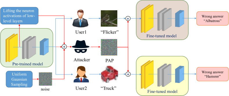
Figure 1: A demonstration of pre-trained adversarial perturbations (PAPs): An attacker first downloads pre-trained weights on the Internet and generates a PAP by lifting the neuron activations of low-level layers of the pre-trained models. We adopt a data augmentation technique called uniform Gaussian sampling to improve the transferability of PAP. When users fine-tune the pre-trained models to complete downstream tasks, the attacker can add the PAP to the input of the fine-tuned models to cheat them without knowing the specific downstream tasks.

In this paper, we introduce Pre-trained Adversarial Perturbations (PAPs), a new kind of universal adversarial perturbations designed for pre-trained models. Specifically, a PAP is generated for a pre-trained model to effectively fool any downstream model obtained by fine-tuning the pre-trained one, as illustrated in Fig. 1. It works under a quasi-black-box setting where the downstream task, dataset, and fine-tuned model parameters are all unavailable. This attack setting is more suitable for the pre-training to the fine-tuning procedure since many pre-trained models are publicly available, and the adversary may generate PAPs before the pre-trained model has been fine-tuned. Although there are many methods [11, 58] proposed for improving the transferability, they do not consider the specific characteristics of the pre-training to the fine-tuning procedure, limiting their cross-finetuning transferability in our setting.

To generate more effective PAPs, we propose a Low-Level Layer Lifting Attack (L4A) method, which aims to lift the feature activations of low-level layers. Motivated by the finding that the lower the level of the model’s layer is, the less its parameters change during fine-tuning, we generate PAPs to destroy the low-level feature representations of pre-trained models, making the attacking effects better reserved after fine-tuning. To further alleviate the overfitting of PAPs to the source domain, we improve L4A with a noise augmentation technique. We conduct extensive experiments on typical pre-trained vision models [4, 21] and ten downstream tasks. The evaluation results demonstrate that our method achieves a higher attack success rate on average compared with the alternative baselines.

2 Related work

Self-supervised learning. Self-supervised learning (SSL) enables learning from unlabeled data. To achieve this, early approaches utilize hand-crafted pretext tasks, including colorization [64], rotation prediction [14], position prediction [45], and Selfie [55]. Another approach for SSL is contrastive learning [32, 48, 4, 26], which aims to map the input image to the feature space and minimize the distance between similar ones while keeping dissimilar ones far away from each other. In particular, a similar sample is retrieved by applying appropriate data augmentation techniques to the original one, and the versions of different samples are viewed as dissimilar pairs.

Adversarial examples. With the knowledge of the structure and parameters of a model, many algorithms [31, 39, 37, 47] successfully fool the target model in a white-box manner. An intriguing property of adversarial examples is their good transferability [33, 40]. The universal adversarial perturbations [40] demonstrate good cross-data transferability by optimizing under a distribution of data samples. The cross-model transferability has also been extensively studied [11, 58, 12], enabling the attack on black-box models without any knowledge of their internal working mechanisms.

Robustness of the pre-training to fine-tuned procedure. Due to the popularity of pre-trained models, a lot of works [53, 60, 6] study the robustness of this setting. Among them, Dong et al. [10] propose a novel adversarial fine-tuning method in an information-theoretical way to retain robust features learned from the pre-trained model. Jiang et al. [24] integrate adversarial samples into the pre-training procedure to defend against attacks. Fan et at. [13] adopt Clusterfit [59] to generate pseudo-label data and later use them for training the model in a supervised way, which improves the robustness of the pre-trained model. The main difference between our work and theirs is that we consider the problem from an attacker’s perspective.

3 Methodology

In this section, we first introduce the notations and the problem formulation of the Pre-trained Adversarial Perturbations (PAPs). Then, we detail the Low-Level Layer Lifting Attack (L4A) method.

3.1 Notations and problem formulation

Let $f_{\boldsymbol{\mathbf{\theta}}}$ denote a pre-trained model for feature extraction with parameters $\boldsymbol{\mathbf{\theta}}$. It takes an image ${\boldsymbol{\mathbf{x}}}$ $\in$ $\mathcal{D}_{p}$ as input and outputs a feature vector ${\boldsymbol{\mathbf{v}}}$ $\in$ $\mathcal{X}$, where $\mathcal{D}_{p}$ and $\mathcal{X}$ refer to the pre-training dataset and feature space, respectively. We denote $f_{\boldsymbol{\mathbf{\theta}}}^{k}({\boldsymbol{\mathbf{x}}})$ as the $k$-th layer’s feature map of $f_{\boldsymbol{\mathbf{\theta}}}$ for an input image ${\boldsymbol{\mathbf{x}}}$. In the pre-training to fine-tuning paradigm, a user fine-tunes the pre-trained model $f_{\boldsymbol{\mathbf{\theta}}}$ using a new dataset $\mathcal{D}_{t}$ of the downstream task and finally gets a fine-tuned model $f_{\boldsymbol{\mathbf{\theta^{\prime}}}}$ with updated parameters ${\boldsymbol{\mathbf{\theta^{\prime}}}}$. Then, let $f_{\boldsymbol{\mathbf{\theta^{\prime}}}}({\boldsymbol{\mathbf{x}}})$ be the predicted probability distribution of an image $\boldsymbol{\mathbf{x}}$ over the classes of $\mathcal{D}_{t}$, and $F_{\boldsymbol{\mathbf{\theta^{\prime}}}}({\boldsymbol{\mathbf{x}}})=\operatorname*{arg\,max}f_{\boldsymbol{\mathbf{\theta^{\prime}}}}({\boldsymbol{\mathbf{x}}})$ be the final classification result.

In this paper, we introduce Pre-trained Adversarial Perturbations (PAPs), which are generated for the pre-trained model $f_{\boldsymbol{\mathbf{\theta}}}$, but can effectively fool fine-tuned models $f_{\boldsymbol{\mathbf{\theta^{\prime}}}}$ on downstream tasks. Formally, a PAP is a universal perturbation $\boldsymbol{\mathbf{\delta}}$ within a small budget $\epsilon$ crafted by $f_{\boldsymbol{\mathbf{\theta}}}$ and $\mathcal{D}_{p}$, such that $F_{\boldsymbol{\mathbf{\theta^{\prime}}}}({\boldsymbol{\mathbf{x}}}+\boldsymbol{\mathbf{\delta}})\neq F_{\boldsymbol{\mathbf{\theta^{\prime}}}}(\boldsymbol{\mathbf{x}})$ for most of the instances belonging to the fine-tuning dataset $\mathcal{D}_{t}$. This can be formulated as the following optimization problem:

$$\max_{\boldsymbol{\mathbf{\delta}}}\mathbb{E}_{{\boldsymbol{\mathbf{x}}}\sim\mathcal{D}_{t}}[F_{\boldsymbol{\mathbf{\theta^{\prime}}}}({\boldsymbol{\mathbf{x}}})\neq F_{\boldsymbol{\mathbf{\theta^{\prime}}}}({\boldsymbol{\mathbf{x}}}+\boldsymbol{\mathbf{\delta}})],\;\text{s.t.}\;\|\boldsymbol{\mathbf{\delta}}\|_{p}\leq\epsilon\;\text{and }{\boldsymbol{\mathbf{x}}}+\boldsymbol{\mathbf{\delta}}\in\left[0,1\right],$$ (1)

where $\|\cdot\|_{p}$ denotes the $\ell_{p}$ norm and we take the $\ell_{\infty}$ norm in this work. There exist some works related to the universal perturbations, such as the universal adversarial perturbation (UAP) [40] and the fast feature fool (FFF) [41], as detailed below.

UAP: Given a classifier $f$ and its dataset $\mathcal{D}$, the UAP tries to generate a perturbation $\boldsymbol{\mathbf{\delta}}$ that can fool the model on most of the instances from $\mathcal{D}$, which is usually solved by an iterative method. Every time sampling an image ${\boldsymbol{\mathbf{x}}}$ from the dataset $\mathcal{D}$, the attacker computes the minimal perturbation $\boldsymbol{\mathbf{\zeta}}$ that sends ${\boldsymbol{\mathbf{x}}}+\boldsymbol{\mathbf{\delta}}$ to the decision boundary by Eq. (2) and then adds it into $\boldsymbol{\mathbf{\delta}}$.

$$\boldsymbol{\mathbf{\zeta}}\leftarrow\arg\min_{\boldsymbol{\mathbf{r}}}\|\boldsymbol{\mathbf{r}}\|_{2},\;\text{s.t.}\;F(\boldsymbol{\mathbf{x}}+\boldsymbol{\mathbf{\delta}}+\boldsymbol{\mathbf{r}})\neq F(\boldsymbol{\mathbf{x}}).$$ (2)

FFF: It aims to produce maximal spurious activations at each layer. To achieve this, FFF starts with a random $\boldsymbol{\mathbf{\delta}}$ and solves the following problem:

$$\min_{\boldsymbol{\mathbf{\delta}}}-\log\left(\prod\limits_{i=0}^{K}\overline{l}_{i}(\boldsymbol{\mathbf{\delta}})\right),\;\text{s.t.}\;\|\boldsymbol{\mathbf{\delta}}\|_{p}\leq\epsilon.$$ (3)

where $\overline{l}_{i}(\boldsymbol{\mathbf{\delta}})$ is the mean of the output tensor at layer $i$.

3.2 Our design

However, these attacks show limited cross-finetuning transferability in our problem setting due to ignorance of the fine-tuning procedure. Two challenges are degenerating the performance.

• Fine-tuning Deviation. The parameters of the model could change a lot during fine-tuning. As a result, the generated adversarial samples may perform well in the feature space of the pre-trained model but fail in the fine-tuned ones.

• Datasets Deviation. The statistics (i.e., mean and standard deviation) of different datasets can vary a lot. Only using the pre-training dataset with the fixed statistics to generate adversarial samples may suffer a performance drop.

To alleviate the negative effect of the above issues, we propose a Low-Level Layer Lifting Attack (L4A) method equipped with a uniform Gaussian sampling strategy.

Low-Level Layer Lifting Attack (L4A). Our method is motivated by the findings in Fig. 2 that the higher the level of the layers, the more their parameters change during fine-tuning. This is also consistent with the knowledge that the low-level convolutional layer acts as an edge detector that extracts low-level features like edges and textures and has little high-level semantic information [46, 61]. Since images from different datasets share the same low-level features, the parameters of these layers can be preserved during fine-tuning. In contrast, the attack algorithms based on the high-level layers or the scores predicted by the model may not transfer well in such a cross-finetuning setting, as the feature spaces of high-level layers are easily distorted during fine-tuning. The basic method of L4A can be formulated as the following problem:

$$\min_{\boldsymbol{\mathbf{\delta}}}L_{base}(f_{\boldsymbol{\mathbf{\theta}}},\boldsymbol{\mathbf{x}},\boldsymbol{\mathbf{\delta}})=-\mathbb{E}_{\boldsymbol{\mathbf{x}}\sim D_{p}}\bigg{[}\|f_{\boldsymbol{\mathbf{\theta}}}^{k}(\boldsymbol{\mathbf{x}}+\boldsymbol{\mathbf{\delta}})\|_{F}^{2}\bigg{]},$$ (4)

where $\|\cdot\|_{F}$ denotes the Frobenius norm of the input tensor. In our experiments, we find the lower the layer, the better it performs, so we choose the first layer as default, such that $k=1$. As Eq. (4) is usually a sophisticated non-convex optimization problem, we solve it using stochastic gradient descent method.

We also find that fusing the adversarial loss of the consecutive low-level layers can boost the performance, which gives L4A_fuse method as solving:

$$\min_{\boldsymbol{\mathbf{\delta}}}L_{fuse}(f_{\boldsymbol{\mathbf{\theta}}},\boldsymbol{\mathbf{x}},\boldsymbol{\mathbf{\delta}})=-\mathbb{E}_{\boldsymbol{\mathbf{x}}\sim D_{p}}\bigg{[}\|f_{\boldsymbol{\mathbf{\theta}}}^{k_{1}}(\boldsymbol{\mathbf{x}}+\boldsymbol{\mathbf{\delta}})\|_{F}^{2}+\lambda\cdot\|f_{\boldsymbol{\mathbf{\theta}}}^{k_{2}}(\boldsymbol{\mathbf{x}}+\boldsymbol{\mathbf{\delta}})\|_{F}^{2}\bigg{]},$$ (5)

where $f_{\boldsymbol{\mathbf{\theta}}}^{k_{1}}(\boldsymbol{\mathbf{x}}+\boldsymbol{\mathbf{\delta}})$ and $f_{\boldsymbol{\mathbf{\theta}}}^{k_{2}}(\boldsymbol{\mathbf{x}}+\boldsymbol{\mathbf{\delta}})$ refers to the $k_{1}$-th and $k_{2}$-th layers’ feature maps of $f_{\boldsymbol{\mathbf{\theta}}}$ respectively, $\lambda$ is a balancing hyperparameter. We set $k_{1}=1$ and $k_{2}=2$ as default.

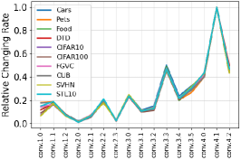
(a) Resnet50

(b) Resnet101

(c) ViT16

Figure 2: The ordinate represents the Frobenius norm of the difference between the parameters of the fine-tuned model and its corresponding pre-trained model, which is scaled into a range from 0 to 1 for easy comparison. The abscissa represents the level of the layer. Note that Resnet50 and Resnet101 [18] are pre-trained by SimCLRv2 [4], and ViT16 [56] is pre-trained by MAE [21].

Figure 3: Datasets’ statistics.

Uniform Gaussian Sampling. Nowadays, most state-of-the-art networks apply batch normalization [23] to input images for better performance. Thus, the datasets’ statistics become an essential factor for training. As shown in Fig. 3, the distribution of the downstream datasets can vary significantly compared to that of the pre-training dataset. However, traditional data augmentation techniques [62, 22] are limited to the pre-training domain and cannot alleviate the problem. Thus, we propose sampling Gaussian noises with various means and deviations to avoid overfitting. Combining the base loss using the pre-training dataset and the new loss using uniform Gaussian noises gives the L4A_ugs method as follows:

$$\min_{\boldsymbol{\mathbf{\delta}}}L_{ugs}(f_{\boldsymbol{\mathbf{\theta}}},\boldsymbol{\mathbf{x}},\boldsymbol{\mathbf{\delta}})=-\mathbb{E}_{\boldsymbol{\mathbf{\boldsymbol{\mathbf{\mu}}}},\boldsymbol{\mathbf{\sigma}},\boldsymbol{\mathbf{n}}_{0}\sim N\left(\boldsymbol{\mathbf{\mu}},\boldsymbol{\mathbf{\sigma}}\right)}\bigg{\{}\mathbb{E}_{\boldsymbol{\mathbf{x}}\sim\mathcal{D}_{p}}\bigg{[}{\|f_{\boldsymbol{\mathbf{\theta}}}^{k}(\boldsymbol{\mathbf{x}}+\boldsymbol{\mathbf{\delta}})\|_{F}^{2}}+\lambda\cdot{\|f_{\boldsymbol{\mathbf{\theta}}}^{k}(\boldsymbol{\mathbf{n}}_{0}+\boldsymbol{\mathbf{\delta}})\|_{F}^{2}}\bigg{]}\bigg{\}},$$ (6)

where $\boldsymbol{\mathbf{\boldsymbol{\mathbf{\mu}}}}$ and $\boldsymbol{\mathbf{\boldsymbol{\mathbf{\sigma}}}}$ are drawn from the uniform distribution $U\left(\boldsymbol{\mathbf{\mu}}_{l},\boldsymbol{\mathbf{\mu}}_{h}\right)$ and $U\left(\boldsymbol{\mathbf{\sigma}}_{l},\boldsymbol{\mathbf{\sigma}}_{h}\right)$, respectively, and $\boldsymbol{\mathbf{\mu}}_{l}$, $\boldsymbol{\mathbf{\mu}}_{h}$, $\boldsymbol{\mathbf{\sigma}}_{l}$, $\boldsymbol{\mathbf{\sigma}}_{r}$ are four hyperparameters.

4 Experiments

We provide some experimental results in this section. More results can be found in Appendix. Our code is publicly available at https://github.com/banyuanhao/PAP.

4.1 Settings

Pre-training methods. SimCLR [4, 5] uses the Resnet [18] backbone and pre-trains the model by contrastive learning. We download pre-trained parameters of Resnet50 and Resnet101 to evaluate the generalization ability of our algorithm on different architectures. We also adopt MOCO [19] with the backbone of Resnet50. Besides convolutional neural networks, transformers [56] attract much attention nowadays for their competitive performance. Based on transformers and masked image modeling, MAE [21] becomes a good alternative for pre-training. We adopt the pre-trained ViT-base-16 model. Moreover, vision-language pre-trained models are gaining popularity these days. Thus we also choose CLIP [51] for our study. We report the results of SimCLR and MAE in Section 4.2. More results on CLIP and MOCO can be found in Appendix A.1.

Table 1: The attack success rate (%) of various attack methods against Resnet101 pre-trained by SimCLRv2. Note that C10 stands for CIFAR10 and C100 stands for CIFAR100.

ASR	Cars	Pets	Food	DTD	FGVC	CUB	SVHN	C10	C100	STL10	AVG
FFFno	43.81	38.62	49.95	63.24	85.57	48.38	12.55	8.53	77.74	57.11	48.55
FFFFmean	33.93	31.37	41.77	52.66	78.94	45.00	14.85	14.42	72.59	56.66	44.22
FFFone	31.87	29.74	39.25	46.92	74.17	43.87	9.24	11.77	65.61	50.21	40.26
DR	36.28	35.54	47.43	47.45	75.00	44.15	12.05	21.35	65.39	41.65	42.63
SSP	32.89	30.50	43.12	45.85	82.57	45.55	8.69	11.66	65.80	40.91	40.75
ASV	60.75	19.84	36.33	56.22	84.16	55.82	7.11	7.29	58.10	80.89	46.64
UAP	48.70	36.55	60.80	63.40	76.06	52.64	8.46	8.53	52.35	31.15	43.86
UAPEPGD	94.12	66.66	61.30	72.55	70.34	82.72	13.88	61.65	20.04	50.13	59.34
L4Abase	94.07	61.57	71.23	69.20	96.28	81.07	11.70	12.68	80.57	90.49	66.89
L4Afuse	90.98	88.53	80.65	74.31	93.79	91.23	11.40	17.40	80.98	89.69	67.10
L4Augs	94.24	94.99	78.28	77.23	92.92	91.77	11.40	14.60	76.50	90.05	72.20

Datasets and Pre-processing. We adopt the ILSVRC 2012 dataset [52] to generate PAPs, which are also used to pre-train the models. We mainly evaluate PAPs on image classification tasks, which are the same as the settings of SimCLRv2. Ten fine-grained and coarse-grained datasets are used to test the cross-finetuning transferability of the generated PAPs. We load these datasets from torchvision (Details in Appendix D). Before feeding the images to the model, we resize them to $256\times 256$ and then center crop them into $224\times 224$.

Compared methods. We choose UAP [40] to test whether image-agnostic attacks also bear good cross-finetuning transferability. Since UAP needs final classification predictions of the inputs, we fit a linear head on the pre-trained feature extractor. Furthermore, by integrating the moment term into the iterative method, UAPEPGD [9] is believed to enhance cross-model transferability. Thus, we adopt UAPEPGD to study the connection between cross-model and cross-finetuning transferability. As our algorithm is based on the feature level, other feature attacks (including FFF [41], ASV [27], DR [35], SSP [43]) are chosen for comparison.

Default settings and Metric. Unless otherwise specified, we choose a batch size of $16$ and a step size of $0.0002$. All the perturbations should be within the bound of $0.05$ under the $\ell_{\infty}$ norm. We evaluate the perturbations at the iterations of $1,000$, $5,000$, $30,000$, and $60,000$, and report the best performance. We show the results in the measure of attack success rates (ASR), representing the classification error rate on the whole testing dataset after adding the perturbations to the legitimate images.

4.2 Main results

We craft pre-trained adversarial perturbations (PAPs) for three pre-trained models (i.e., Resnet50 by SimCLRv2, Resnet101 by SimCLRv2, ViT16 by MAE) and evaluate the attack success rates on ten downstream tasks. The results are shown in Table 1, Table 2, and Table 3, respectively. Note that the first seven datasets are fine-grained, while the last three are coarse-grained ones. We mark the best results for each dataset in bold, and the best baseline in blue. We highlight the results of L4A_ugs in red to emphasize that the L4A attack equipped with Uniform Gaussian Sampling shows great cross-finetuning transferability and performs best.

Table 2: The attack success rate (%) of various attack methods against Resnet50 pre-trained by SimCLRv2. Note that C10 stands for CIFAR10, and C100 stands for CIFAR100.

ASR	Cars	Pets	Food	DTD	FGVC	CUB	SVHN	C10	C100	STL10	AVG
FFFno	26.91	30.83	43.28	48.99	41.30	38.23	79.00	68.50	44.67	16.95	43.86
FFFmean	36.75	33.88	45.26	50.15	53.13	77.22	52.02	82.41	68.10	22.11	52.10
FFFone	37.88	35.30	52.79	59.52	59.62	57.04	80.33	75.40	53.58	18.31	52.98
DR	38.64	34.42	50.04	45.53	39.80	75.67	47.88	76.05	60.57	13.98	48.26
SSP	41.70	43.94	50.83	48.78	47.67	82.39	48.38	86.95	66.23	19.56	53.64
ASV	74.47	36.93	45.85	73.51	64.89	92.29	73.16	45.14	53.60	22.02	58.19
UAP	44.86	46.47	64.67	65.53	49.63	82.32	52.00	79.63	46.46	19.99	55.16
UAPEPGD	66.29	66.58	81.11	69.52	87.91	59.07	69.16	87.84	68.26	37.12	69.28
LLLLbase	94.86	56.30	61.31	75.37	67.61	94.87	81.45	68.25	77.04	34.56	66.89
L4Afuse	96.00	59.80	65.00	77.93	69.39	95.02	85.05	64.41	76.29	37.54	72.64
L4Augs	96.13	79.15	74.87	82.18	78.73	94.45	95.29	55.03	77.10	45.09	77.80

Table 3: The attack success rate (%) of various attack methods against ViT16 pre-trained by MAE. Note that C10 stands for CIFAR10 and C100 stands for CIFAR100.

ASR	Cars	Pets	Food	DTD	FGVC	CUB	SVHN	C10	C100	STL10	AVG
FFFno	64.31	88.21	95.04	88.18	81.91	92.94	76.10	49.48	79.83	60.91	77.69
FFFmean	40.39	67.54	54.10	61.38	71.47	73.39	92.96	86.88	94.55	67.90	71.06
FFFone	48.36	77.89	60.06	64.04	75.67	74.09	92.33	86.13	94.48	70.40	74.35
DR	37.02	23.84	59.54	44.73	28.01	10.41	14.30	16.66	14.12	21.54	27.02
SSP	44.15	73.31	85.42	72.82	52.57	63.10	52.45	27.94	25.32	36.90	53.40
ASV	38.46	10.17	37.49	48.31	29.14	4.97	8.41	17.04	11.34	21.14	22.64
UAP	62.71	58.90	89.90	74.92	44.69	39.56	47.65	47.77	33.80	51.70	55.16
UAPEPGD	63.67	73.09	96.22	76.69	57.78	73.37	79.84	45.89	47.21	55.79	66.95
L4Abase	87.66	89.98	98.96	99.10	99.33	84.06	86.99	98.62	97.08	98.25	94.00
L4Afuse	83.24	89.57	98.87	98.77	98.36	93.60	89.85	98.64	95.72	97.53	94.42
L4Augs	96.49	90.00	98.97	98.89	99.48	84.01	89.56	99.43	97.27	98.96	95.30

A quick glimpse shows that our proposed methods outperform all the baselines by a large margin. For example, as can be seen from Table 1, if the target model is Resnet101 pre-trained by SimCLRv2, the best competitor FFF_mean achieves an average attack success rate of 59.34%, while the villain L4A_base can lift it up to 66.89% and the UGS technique further boosts the performance up to 72.20%. Moreover, the STL10 dataset is the hardest for PAPs to transfer among these tasks. However, L4A_ugs can significantly improve the cross-finetuning transferability, achieving an attack success rate of 90.05% and 98.96% for Resnet101 and ViT16 in STL10, respectively. Another intriguing finding is that ViT16 with a transformer backbone shows severe vulnerabilities to PAPs. Although performing best on legitimate samples, they bear an attack success rate of 95.30% under the L4A_ugs attack, closing to random outputs. These results reveal the serious security problem of the pre-training to fine-tuning paradigm and demonstrate the effectiveness of our method in such a problem setting.

4.3 Ablation studies

4.3.1 Effect of the attacking layer

We analyze the influence of attacking different intermediate layers of the networks on the performance of our proposed L4A_base in the pre-training domain (ImageNet) and the fine-tuning domains (ten downstream tasks). To this end, we divide Resnet50, Resnet101, and ViT into five blocks (Details in Appendix F.1) and conduct our algorithm on them. Note that for the fine-tuning domains, the average attack success rates on the ten datasets are reported.

As shown in Fig. 4, the lower the level we choose to attack, the better our algorithm performs in the fine-tuning domains. Moreover, for the pre-training domain, attacking the middle layers of the networks results in a higher attack success rate compared to the top and bottom layers, which is also reported in existing works [36, 43, 63]. These results reveal the intrinsic property of the pre-training to fine-tuning paradigm. As the lower-level layers change less during the fine-tuning procedure, attacking the low-level layer becomes more effective when generating adversarial perturbations in the pre-training domain rather than the middle-level layers.

Figure 4: The attack success rates (%) of L4A_base when using different layers. We show the results on the pre-training domain (Left) and fine-tuning domains (Right).

4.3.2 Effect of uniform Gaussian sampling

We set $\boldsymbol{\mathbf{\mu}}_{l},\boldsymbol{\mathbf{\mu}}_{h},\boldsymbol{\mathbf{\sigma}}_{l},\boldsymbol{\mathbf{\sigma}}_{h}$ as 0.4, 0.6, 0.05, 0.1 for all the three models as they perform best. To discuss the effect of the hyperparameter $\lambda$ in Eq. (6) fusing the base loss and the UGS loss, we select the values with a grid of 8 logarithmically spaced learning rates between $10^{-2}$ and $10^{2}$. The results are shown in Fig. 5. As shown in Fig. 5(a), the best attack success rate is achieved when $\lambda=10^{-0.5}$ on Resnet101, boosting the performance by 1.52% compared to only using the Gaussian noises.

(a) Resnet101

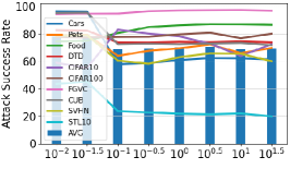
(b) Resnet50

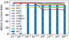
(c) ViT16

Figure 5: The attack success rate (%) of different hyperparameter $\lambda$ in L4A_ugs for different models.

Table 4: Fixed datasets’ statistics

Model	R101	R50	MAE
None	66.95	71.16	94.00
ImageNet	68.39	69.50	95.30
Uniform	72.20	77.80	95.30

Furthermore, we study whether adopting the fixed statistics of the pre-training dataset (i.e., the mean and standard deviation of ImageNet) can help. We report the attack success rates (%) in the Table 4, where None refers to using no data augmentation, ImageNet adopts the mean and standard deviation of ImageNet and Uniform samples a pair of mean and standard deviation from the uniform distribution. As can be seen from the table, Uniform outperforms None by 4.39% on average, while ImageNet does not help, which means that our proposed UGS helps to avoid overfitting the pre-training domain.

4.4 Visualization of feature maps

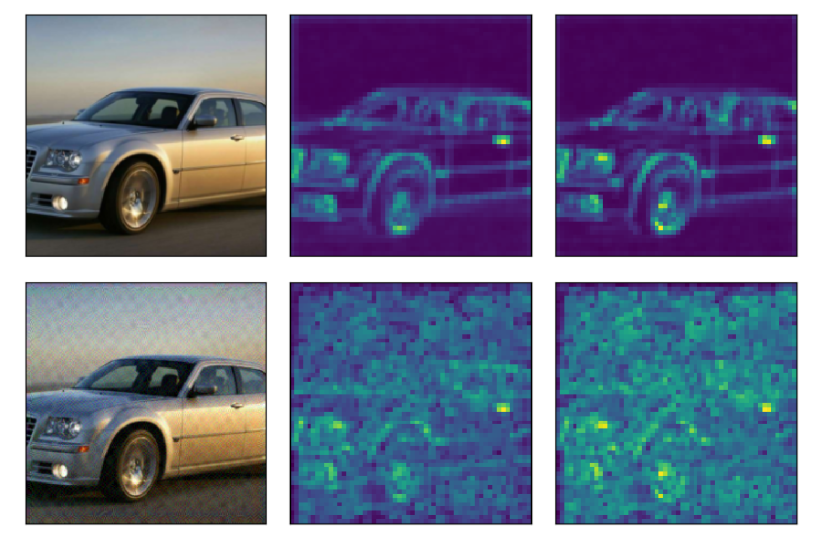
Figure 6: Visualization of feature maps.

We show the feature maps before and after L4A_fuse attack in Fig. 6. The Left column shows the inputs of the model, while the Middle and the Right show the feature map of the pre-trained model and the fine-tuned one, respectively. The Upper row represents the pipeline of a clean input in Cars, and the Lower shows that of adversarial ones. We can see from the upper row that fine-tuning the model can make it sensitive to the defining features related to the specific domain, such as tires and lamps. However, adding an adversarial perturbation to the image can significantly lift all the activations and finally mask the useful features. Moreover, the effect of our attack could be well preserved during fine-tuning and cheat the fine-tuned model into misclassification, stressing the safety problem of pre-trained models.

4.5 Trade-off between the clean accuracy and robustness

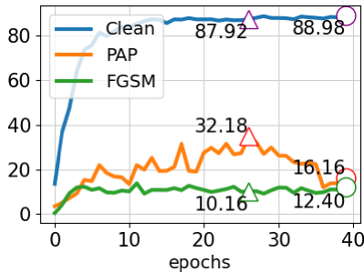
(a) Pets

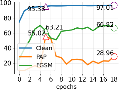
(b) STL10

Figure 7: Model accuracy (%) on the Pets and STL10 datasets under clean inputs, PAP, and FGSM attack.

We study the effect of fine-tuning epochs on the performance of our attack. To this end, we fine-tune the model until it reports the best result on the testing dataset, and then we plot the clean accuracy and the accuracy against FGSM and PAPs on Pets and STL10 in Fig. 7. The figure shows the clean accuracy and robustness of the fine-tuned model against PAPs are at odds. In Fig. 7(b), the model shows the best robustness at epoch 5 in STL10, achieving an accuracy rate of 95.38% and 55.02% on clean and adversarial samples, respectively. However, the model does not converge until epoch 19. Though the process boosts the clean accuracy by 1.63%, it suffers a significant drop in robustness, as the accuracy on adversarial samples is lowered to 28.96%. Such findings reveal the safety problem of the pre-training to fine-tuning paradigm.

5 Discussion

In this section, we first introduce the gradient alignment and then use it to explain the effectiveness of our method. In particular, we show why our algorithms fall behind UAPs in the pre-training domain but have better cross-finetuning transferability when evaluated on the downstream tasks.

5.1 Preliminaries

Gradient sequences. Given a network $f_{{\boldsymbol{\mathbf{\theta}}}_{0}}$ and a sample sequence $\{\boldsymbol{\mathbf{x}}_{1}\,\boldsymbol{\mathbf{x}}_{2},\boldsymbol{\mathbf{x}}_{3},...,\boldsymbol{\mathbf{x}}_{N}\}_{\mathcal{D}}$ drawn from the dataset $\mathcal{D}$, let $\Delta\boldsymbol{\mathbf{\delta}}_{\boldsymbol{\mathbf{\theta}}_{0},\mathcal{D}}=\{\Delta\boldsymbol{\mathbf{\delta}}_{\boldsymbol{\mathbf{\theta}}_{0},\boldsymbol{\mathbf{x}}_{1}},\Delta\boldsymbol{\mathbf{\delta}}_{\boldsymbol{\mathbf{\theta}}_{0},\boldsymbol{\mathbf{x}}_{2}},\Delta\boldsymbol{\mathbf{\delta}}_{\boldsymbol{\mathbf{\theta}}_{0},\boldsymbol{\mathbf{x}}_{3}},...,\Delta\boldsymbol{\mathbf{\delta}}_{\boldsymbol{\mathbf{\theta}}_{0},\boldsymbol{\mathbf{x}}_{N}}\}_{\mathcal{D}}$ be the sequence of gradients obtained when generating adversarial samples by the following equation:

$$\Delta\boldsymbol{\mathbf{\delta}}_{\boldsymbol{\mathbf{\theta}}_{0},{\boldsymbol{\mathbf{x}}}_{i}}=\nabla_{\boldsymbol{\mathbf{\delta}}}L(f_{\boldsymbol{\mathbf{\theta}}_{0}},{\boldsymbol{\mathbf{x}}}_{i},{\boldsymbol{\mathbf{\delta}}}_{i}),\;\text{with }{\boldsymbol{\mathbf{\delta}}}_{i}=P_{\infty,\boldsymbol{\mathbf{\epsilon}}}(\boldsymbol{\mathbf{\delta}}_{i-1}+\Delta\boldsymbol{\mathbf{\delta}}_{\boldsymbol{\mathbf{\theta}}_{0},{\boldsymbol{\mathbf{x}}}_{i-1}}),$$ (7)

where $L$ denotes the loss function of iterative attack methods like UAP, FFF, and L4A.

Definition 1 (Gradient alignment).

Given a dataset ${\mathcal{D}}$ and a model $f_{\boldsymbol{\mathbf{\theta}}_{0}}$, the gradient alignment ${\mathcal{GA}}$ of an attack algorithm is defined as the expectation over the cosine similarity of $\Delta\boldsymbol{\mathbf{\delta}}_{\boldsymbol{\mathbf{\theta}}_{0},\boldsymbol{\mathbf{x}}_{1}}$ and $\Delta\boldsymbol{\mathbf{\delta}}_{\boldsymbol{\mathbf{\theta}}_{0},\boldsymbol{\mathbf{x}}_{2}}$, which can be formulated as Eq. (8)

$$\mathcal{GA}=\mathbb{E}_{\boldsymbol{\mathbf{x}}_{1}\sim\mathcal{D},\boldsymbol{\mathbf{x}}_{2}\sim\mathcal{D}}\left[\frac{\Delta\boldsymbol{\mathbf{\delta}}_{\boldsymbol{\mathbf{\theta}}_{0},\boldsymbol{\mathbf{x}}_{1}}\cdot{\Delta\boldsymbol{\mathbf{\delta}}_{\boldsymbol{\mathbf{\theta}}_{0},\boldsymbol{\mathbf{x}}_{2}}}}{\|\Delta\boldsymbol{\mathbf{\delta}}_{\boldsymbol{\mathbf{\theta}}_{0},\boldsymbol{\mathbf{x}}_{1}}\|_{2}\cdot\|{\Delta\boldsymbol{\mathbf{\delta}}_{\boldsymbol{\mathbf{\theta}}_{0},\boldsymbol{\mathbf{x}}_{2}}}\|_{2}}\right],$$ (8)

where $\Delta\boldsymbol{\mathbf{\delta}}_{\boldsymbol{\mathbf{\theta}}_{0},\boldsymbol{\mathbf{x}}_{1}}$ and $\Delta\boldsymbol{\mathbf{\delta}}_{\boldsymbol{\mathbf{\theta}}_{0},\boldsymbol{\mathbf{x}}_{2}}$ are two consecutive elements obtained by Eq. (7).

Then the L4A algorithm bears a higher gradient alignment (A strict definition and proof in a weaker form can be found in Appendix B.1). In addition, we provide the results of a simulation experiment to justify it in Table 5.1. We can see a negative correlation between the gradient alignment and the attack success rate on ImageNet. In contrast, a positive correlation exists between the gradient alignment and attack success rate in the fine-tuning domain.

Effectiveness of the algorithm. Given a pre-trained model $f_{\boldsymbol{\mathbf{\theta}}}$ and the pre-training dataset $\mathcal{D}_{p}$, the generation of PAPs can be reformulated from Eq. (1) to the following equation:

$$\max_{\boldsymbol{\mathbf{\delta}}\in\;Span\{\Delta\boldsymbol{\mathbf{\delta}}_{\boldsymbol{\mathbf{\theta}},\mathcal{D}_{p}}\}}\mathbb{E}_{{\boldsymbol{\mathbf{x}}}\sim\mathcal{D}_{t}}[F_{\boldsymbol{\mathbf{\theta}}^{\prime}}({\boldsymbol{\mathbf{x}}})\neq F_{\boldsymbol{\mathbf{\theta}}^{\prime}}({\boldsymbol{\mathbf{x}}}+\boldsymbol{\mathbf{\delta}})],\;\text{s.t.}\;\|\boldsymbol{\mathbf{\delta}}\|_{p}\leq\epsilon\;\text{and }{\boldsymbol{\mathbf{x}}}+\boldsymbol{\mathbf{\delta}}\in\left[0,1\right],$$ (9)

where $Span\{\Delta\boldsymbol{\mathbf{\delta}}_{\boldsymbol{\mathbf{\theta}},\mathcal{D}_{p}}\}$ denotes the subspace spanned by the elements of $\Delta\boldsymbol{\mathbf{\delta}}_{\boldsymbol{\mathbf{\theta}},\mathcal{D}_{p}}$. The optimal value $\boldsymbol{\mathbf{\delta}}$ can be viewed as a linear combination of the elements in $\Delta\boldsymbol{\mathbf{\delta}}_{\boldsymbol{\mathbf{\theta}},\mathcal{D}_{p}}$, so it is the feasible region of the equation. In particular, the feasible region of Eq. (9) is smaller than that of Eq. (1), which reflects that the stochastic gradient descent methods may not converge to the global maximum when it is not included in $Span\{\Delta\boldsymbol{\mathbf{\delta}}_{\boldsymbol{\mathbf{\theta}},\mathcal{D}_{p}}\}$ and the local maximum of Eq. (9) in $Span\{\Delta\boldsymbol{\mathbf{\delta}}_{\boldsymbol{\mathbf{\theta}},\mathcal{D}_{p}}\}$ represents the effectiveness of the algorithm in the fine-tuning domain.

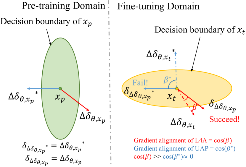
Figure 8: Illustration

Resnet101	${\mathcal{GA}}$	ImageNet	AVG
FFFno	0.1221	38.64%	48.55%
FFFmean	0.0194	48.37%	44.22%
FFFone	0.1222	34.15%	40.26%
DR	0.0165	41.06%	42.62%
UAP	0.0018	88.14%	43.86%
UAPEPGD	0.0008	94.62%	59.39%
SSP	0.0274	41.81%	40.75%
L4Abase	0.6125	37.44%	66.95%

Table 5: Left: Gradient alignments; Middle: Attack success rates on the pre-training dataset; Right: Average attack success rates on downstream tasks. See more details in Appendix B.2

5.2 Explanation

We aim to explain why the effectiveness of our algorithm is better in the fine-tuning domain and worse in the pre-training domain, as seen from Table 5.1. Let $\Delta\boldsymbol{\mathbf{\delta}}_{\boldsymbol{\mathbf{\theta}},\mathcal{D}_{p}}$ and $\Delta\boldsymbol{\mathbf{\delta}}_{\boldsymbol{\mathbf{\theta}},\mathcal{D}_{p}}^{*}$ be the feasible zones of L4A and UAP obtained by feeding instances from $D_{p}$ into the pre-trained model $f_{\boldsymbol{\mathbf{\theta}}}$, respectively. Similarly, we can define $\Delta\boldsymbol{\mathbf{\delta}}_{\boldsymbol{\mathbf{\theta}},\mathcal{D}_{t}}$ and $\Delta\boldsymbol{\mathbf{\delta}}_{\boldsymbol{\mathbf{\theta}},\mathcal{D}_{t}}^{*}$. Meanwhile, denote $\boldsymbol{\mathbf{\delta}}_{\Delta\boldsymbol{\mathbf{\delta}}_{\boldsymbol{\mathbf{\theta}},\mathcal{D}_{p}}}$ and $\boldsymbol{\mathbf{\delta}}_{\Delta\boldsymbol{\mathbf{\delta}}_{\boldsymbol{\mathbf{\theta}},\mathcal{D}_{p}}}^{*}$ as the maxima in the pre-training domain obtained by L4A and UAP respectively. An illustration is shown in Fig. 5.1, supposing there is only one step in the iterative method.

Pre-training domain: Because the gradients of UAP obtained by Eq. (2) represent the directions to the closest points on the decision boundary in the pre-training domain. Thus, limiting the feasible zone to $\Delta\boldsymbol{\mathbf{\delta}}_{\boldsymbol{\mathbf{\theta}},\mathcal{D}_{p}}^{*}$ does little harm to the performance when evaluated in the pre-training domain. Meanwhile, according to the optimal objective, L4A finds the next best directions which are worse than those of UAPs. Thus, $\boldsymbol{\mathbf{\delta}}_{\Delta\boldsymbol{\mathbf{\delta}}_{\boldsymbol{\mathbf{\theta}},\mathcal{D}_{p}}}^{*}$ performs better than $\boldsymbol{\mathbf{\delta}}_{\Delta\boldsymbol{\mathbf{\delta}}_{\boldsymbol{\mathbf{\theta}},\mathcal{D}_{p}}}$ in the pre-training domain.

Fine-tuning domain: According to the fact that UAP bears a low gradient alignment near to 0, the subspace spanned by the tensors in $\Delta\boldsymbol{\mathbf{\delta}}_{\boldsymbol{\mathbf{\Delta}}_{\boldsymbol{\mathbf{\theta}},\mathcal{D}_{p}}}^{*}$ is almost orthogonal to that spanned by the tensors in $\Delta\boldsymbol{\mathbf{\delta}}_{\boldsymbol{\mathbf{\Delta}}_{\boldsymbol{\mathbf{\theta}},\mathcal{D}_{t}}}^{*}$ which represent the best directions that send the sample to the decision boundary in the fine-tuning domain. Thus, limiting the feasible zone of Eq. (1) to $\Delta\boldsymbol{\mathbf{\delta}}_{\boldsymbol{\mathbf{\theta}},\mathcal{D}_{p}}^{*}$ suffers a great drop in ASR when evaluated on the downstream tasks in Eq. (9). However, as shown in Table 5.1, our algorithm can achieve a gradient alignment of up to 0.6125, which means that there is considerable overlap in the next best feasible region of $\mathcal{D}_{p}$ in the pre-training domain obtained by L4A and that of $\mathcal{D}_{f}$ in the fine-tuning domain. Thus the performance of the best solution in $\Delta\boldsymbol{\mathbf{\delta}}_{\boldsymbol{\mathbf{\theta}},\mathcal{D}_{p}}$ is close to that of $\Delta\boldsymbol{\mathbf{\delta}}_{\boldsymbol{\mathbf{\theta}},\mathcal{D}_{f}}$, which represents the next best solution in the fine-tuning domain. Finally we have $\boldsymbol{\mathbf{\delta}}_{\Delta\boldsymbol{\mathbf{\delta}}_{\boldsymbol{\mathbf{\theta}},\mathcal{D}_{p}}}$ performs better than $\boldsymbol{\mathbf{\delta}}_{\Delta\boldsymbol{\mathbf{\delta}}_{\boldsymbol{\mathbf{\theta}},\mathcal{D}_{p}}}^{*}$ in the fine-tuning domain.

In conclusion, the high gradient alignment guarantees high cross-finetuning transferability.

6 Societal impact

A potential negative societal impact of L4A is that malicious adversaries could use it to cause security/safety issues in real-world applications. As more people focus on the pre-trained models because of their excellent performance, fine-tuning pre-trained models provided by the cloud server becomes a panacea for deep learning practitioners. In such settings, PAPs become a significant security flaw–as one can easily access the prototype pre-trained models and perform attacking algorithms on them. Our work appeals to big companies to delve further into the safety problem related to the vulnerability of pre-trained models.

7 Conclusion

In this paper, we address the safety problem of pre-trained models. In particular, an attacker can use them to generate so-called pre-trained adversarial perturbations, achieving a high success rate on the fine-tuned models without knowing the victim model and the specific downstream tasks. Considering the inner qualities of the pre-training to fine-tuning paradigm, we propose a novel algorithm, L4A, which performs well in such problem settings. A limitation of L4A is that it performs worse than UAPs in the pre-training domain; we hope some upcoming work can fill the gap. Furthermore, L4A only utilizes the information in the pre-training domain. When the attacker obtains some information about the downstream tasks, like several unlabeled instances in the fine-tuning domain, he may be able to enhance PAPs using the knowledge and further exacerbate the situation, which we leave to future work. Thus, we hope our work can draw attention to the safety problem of pre-trained models to guarantee security.

Checklist

1. For all authors…

   1. Do the main claims made in the abstract and introduction accurately reflect the paper’s contributions and scope? [Yes]

   2. Did you describe the limitations of your work? [Yes] See Section 7.

   3. Did you discuss any potential negative societal impacts of your work? [Yes] See Section 7.

   4. Have you read the ethics review guidelines and ensured that your paper conforms to them? [Yes]

2. If you are including theoretical results…

   1. Did you state the full set of assumptions of all theoretical results? [N/A]

   2. Did you include complete proofs of all theoretical results? [N/A]

3. If you ran experiments…

   1. Did you include the code, data, and instructions needed to reproduce the main experimental results (either in the supplemental material or as a URL)? [Yes] See Appendix.

   2. Did you specify all the training details (e.g., data splits, hyperparameters, how they were chosen)? [Yes] See Section 4 and Appendix F.

   3. Did you report error bars (e.g., with respect to the random seed after running experiments multiple times)? [No] Since running L4A on all the ten dataset and the three models is time-consuming, we only ran one time.

   4. Did you include the total amount of compute and the type of resources used (e.g., type of GPUs, internal cluster, or cloud provider)? [Yes] See Appendix F.

4. If you are using existing assets (e.g., code, data, models) or curating/releasing new assets…

   1. If your work uses existing assets, did you cite the creators? [Yes]

   2. Did you mention the license of the assets? [Yes] See Appendix D.

   3. Did you include any new assets either in the supplemental material or as a URL? [Yes] See supplementary material.

   4. Did you discuss whether and how consent was obtained from people whose data you’re using/curating? [Yes] See Appendix D.

   5. Did you discuss whether the data you are using/curating contains personally identifiable information or offensive content? [Yes] See Appendix D.

5. If you used crowdsourcing or conducted research with human subjects…

   1. Did you include the full text of instructions given to participants and screenshots, if applicable? [N/A]

   2. Did you describe any potential participant risks, with links to Institutional Review Board (IRB) approvals, if applicable? [N/A]

   3. Did you include the estimated hourly wage paid to participants and the total amount spent on participant compensation? [N/A]

Appendix A Additional experiments

A.1 Additional experiments on other pre-trained models

In this section, we report the results on CLIP and MOCO in Table 6 and Table 7, respectively. Note that the first seven columns of validation datasets are fine-grained, while the next three are coarse-grained ones. We mark the best results for each dataset in bold, and the best baseline in blue. We highlight the results of L4A_ugs in red to emphasize that the Low-Lever Layer Lifting attack equipped with Uniform Gaussian Sampling shows great cross-finetuning transferability and performs best.
These tables show that our proposed methods outperform all the baselines by a large margin. For example, as can be seen from Table 6, if the target model is Resnet50 pre-trained by MOCO, the best competitor UAP achieves an average attack success rate of 54.34%, while the L4A_fuse can lift it up to 54.72% and the UGS technique further boosts the performance up to 59.72%.

Table 6: The attack success rate(%) of various methods we study against Resnet50 pretrained by MOCO. Note that C10 stands for CIFAR10, and C100 stands for CIFAR100.

ASR	Cars	Pets	Food	DTD	FGVC	CUB	SVHN	C10	C100	STL10	AVG
FFFno	30.72	25.59	60.03	48.51	84.97	62.82	4.92	17.22	55.37	12.84	40.30
FFFmean	39.04	32.49	68.94	52.93	85.57	68.93	8.02	22.23	67.53	14.26	45.99
FFFone	31.82	27.26	53.06	51.38	77.92	54.42	5.09	17.43	57.26	10.23	38.59
DR	44.30	39.63	51.11	53.51	81.43	55.85	5.01	30.24	74.25	13.91	44.92
SSP	33.75	36.44	75.32	60.00	80.32	68.73	5.90	25.42	69.27	29.03	48.42
ASV	40.01	32.27	60.63	47.50	82.87	62.77	41.71	11.15	50.30	9.05	43.83
UAP	61.00	52.44	77.00	60.75	83.79	68.54	5.75	28.02	68.22	37.94	54.34
UAPEPGD	45.55	38.05	70.12	54.79	69.04	57.25	3.82	10.47	48.38	21.44	41.89
L4Abase	44.10	51.86	77.44	62.61	81.49	61.30	5.65	45.70	81.88	27.33	53.94
L4Afuse	44.25	54.02	78.09	63.19	82.90	63.26	5.13	46.71	81.66	27.95	54.72
L4Augs	61.22	58.11	86.52	67.71	88.96	65.57	5.08	39.23	83.12	41.93	59.74

Table 7: The attack success rate(%) of various methods we study against Resnet50 pretrained by CLIP. Note that C10 stands for CIFAR10, and C100 stands for CIFAR100.

ASR	Cars	Pets	Food	DTD	FGVC	CUB	SVHN	C10	C100	STL10	AVG
FFFno	89.96	90.41	94.57	82.45	87.81	99.08	98.50	78.20	80.41	89.19	89.06
FFFmean	92.86	89.78	93.28	81.49	89.30	99.00	99.10	75.35	80.41	89.71	89.03
FFFone	89.21	86.73	93.47	80.32	85.63	99.03	98.38	71.78	80.41	84.89	86.98
DR	71.84	52.74	77.07	70.32	86.69	99.01	94.69	61.74	80.41	84.06	77.86
SSP	85.61	84.98	83.23	78.19	90.00	98.98	98.50	75.80	80.41	87.90	86.36
ASV	91.04	90.80	93.98	81.82	88.96	98.02	97.68	78.75	79.41	87.34	88.78
UAP	75.84	65.84	87.12	73.40	88.08	99.00	96.52	57.18	80.41	87.03	81.04
UAPEPGD	64.15	52.14	60.35	67.23	89.99	98.59	95.14	47.05	80.41	80.86	73.59
L4Abase	79.83	66.61	79.74	70.53	85.96	99.03	98.04	64.00	84.01	82.26	81.00
L4Afuse	96.57	96.27	98.39	86.01	88.11	99.00	98.41	80.41	80.95	90.01	91.41
L4Augs	97.12	97.19	98.67	91.12	91.56	99.02	99.10	96.55	80.41	85.36	93.61

A.2 PAPs against adversarial fine-tuned models

In our paper, we only conduct experiments on standard fine-tuning. We followed the training process introduced by [10], which adopts a distillation term to preserve high-quality features of the pretrained model to boost model performance from a view of information theory. We do some additional experiments on Resnet50 pretrained by SimCLRv2. And the results are as follows.

Table 8: The attack success rate(%) of different methods against adversarial fine-tuned models. Note that C10 stands for CIFAR10 and C100 stands for CIFAR100.

ASR	Cars	Pets	Food	DTD	FGVC	CUB	SVHN	C10	C100	STL10	AVG
FFFno	14.69	26.08	50.86	48.40	27.68	31.74	34.35	36.78	10.30	16.56	29.74
FFFmean	14.72	26.30	50.36	48.14	27.70	31.90	33.93	36.74	9.97	16.61	29.64
FFFone	14.65	26.53	53.08	48.52	27.06	31.49	34.02	37.35	10.99	16.73	30.04
DR	14.33	26.96	50.84	47.13	27.39	32.41	33.81	37.39	10.85	16.30	29.74
SSP	14.31	26.08	50.01	48.08	27.51	32.10	33.14	37.14	11.20	16.34	29.59
ASV	11.95	16.35	25.37	37.23	24.58	26.93	32.22	31.39	6.32	7.15	21.95
UAP	14.54	25.67	47.92	48.19	27.34	32.60	33.60	36.71	10.94	16.26	29.38
UAPEPGD	14.40	24.20	46.82	47.18	27.32	32.53	34.02	35.29	10.38	15.51	28.77
L4Abase	14.48	26.76	55.66	50.69	26.22	32.14	33.45	37.33	11.10	16.75	30.46
L4Afuse	14.64	28.07	55.59	50.74	26.96	32.49	33.57	37.66	11.31	16.94	30.80
L4Augs	14.35	25.84	53.79	50.16	26.80	32.02	33.54	36.52	10.81	16.56	30.04

As seen from the table, all the methods suffer degenerated performance against adversarial fine-tuning. However, L4A still performs best among these competitors. For example, considering the DTD dataset, the best baseline FFF_one achieves an attack success rate of 48.52%, while the ASR of the villain L4A_base is up to 50.69%, and the fusing loss further boosts the performance to 50.74%.

A.3 PAPs against adversarial pretrained models

To test PAPs against adversarial pretrained models, we follow the method proposed by [24], which uses adversarial views to boost robustness. We first train a robust Resnet50 using enhanced SimCLRv2. Then, we generate PAPs using that model and test them on both the adversarial fine-tuned and standard fine-tuned models on downstream tasks. In Table 9, we report the results on standard finetuned models.

Table 9: The attack success rate(%) of different methods against adversarial-pretrained-standard-finetuned models. Note that C10 stands for CIFAR10, and C100 stands for CIFAR100.

ASR	Cars	Pets	Food	DTD	FGVC	CUB	SVHN	C10	C100	STL10	AVG
FFFno	45.34	23.33	53.16	44.95	67.63	45.89	81.12	60.78	95.38	18.48	53.61
FFFmean	50.81	27.86	60.99	46.97	74.56	52.69	81.27	71.33	99.00	28.97	59.45
FFFone	44.37	25.21	47.12	46.65	68.35	43.89	81.50	63.36	97.78	15.10	53.33
DR	48.81	34.15	61.32	48.30	79.98	51.36	76.29	63.17	80.29	13.22	55.69
SSP	44.67	34.23	44.84	48.72	69.79	45.32	83.32	81.44	97.95	20.95	54.21
ASV	47.94	25.32	56.66	45.80	65.94	41.14	78.52	61.25	96.17	12.16	53.09
UAP	35.03	32.65	38.39	46.44	67.12	42.22	78.72	67.66	93.81	36.41	53.84
UAPEPGD	23.20	17.85	25.20	39.10	53.47	31.19	66.41	13.63	66.98	6.33	34.33
L4Abase	55.93	26.41	67.82	52.55	79.60	56.64	84.07	84.52	99.00	28.16	63.47
L4Afuse	67.08	25.94	67.95	54.04	82.20	61.41	84.05	83.09	99.00	33.71	65.85
L4Augs	82.46	25.91	74.37	51.65	88.93	72.14	84.08	78.66	98.98	31.97	68.91

The above table shows that adversarial-pretrained models show little robustness after standard fine-tuning, which is also reported in [3, 30]. In such settings, L4A still performs best among these competitors: the best baseline FFF_mean achieves an average attack success rate of 59.45%, while the ASR of the villain L4A_base is up to 63.47%, and the Uniform Gaussian sampling further boosts the performance to 68.91%. Another interesting finding is that low-level-based methods, such as FFF, DR, SSP and L4A, perform better than high-level-based ones like UAPEPGD, which uses classification scores. This further supports our findings in Fig 2 and our motivation to use low-level layers.

In Table 10, we report the results on adversarial-finetuned models. Note that we adopt the adversarial-finetuning method in [10].

Table 10: The attack success rate(%) of different methods against adversarial-pretrained-adversarial-fine-tuned models. Note that C10 stands for CIFAR10, and C100 stands for CIFAR100.

ASR	Cars	Pets	Food	DTD	FGVC	CUB	SVHN	C10	C100	STL10	AVG
FFFno	14.82	27.13	47.84	49.19	37.61	38.82	9.24	21.27	39.32	16.60	30.18
FFFmean	14.88	27.09	48.82	49.40	38.01	38.80	9.09	20.45	39.32	16.47	30.23
FFFone	14.95	27.25	47.08	49.40	37.80	39.01	9.02	21.09	39.31	16.31	30.12
DR	15.18	28.59	48.51	48.30	38.46	38.73	8.64	20.73	39.61	16.86	30.36
SSP	15.20	28.67	39.93	46.38	38.88	37.42	7.35	21.89	39.49	15.11	29.03
ASV	15.56	27.77	49.17	49.15	38.58	37.83	10.16	18.82	34.71	13.44	29.52
UAP	15.53	27.77	48.23	46.96	38.55	37.59	7.49	15.64	35.30	14.43	28.75
UAPEPGD	15.00	28.24	41.39	46.49	37.98	37.04	6.69	11.75	35.02	12.44	27.20
L4Abase	15.64	29.59	49.18	51.65	38.01	39.83	11.24	24.43	38.39	16.96	31.49
L4Afuse	15.90	30.88	49.83	49.89	38.01	40.05	10.69	24.25	37.20	17.10	31.38
L4Augs	15.69	30.25	49.59	52.02	37.68	39.87	11.25	24.52	38.06	17.11	31.60

From Table 10, we can see that adversarial-pretrained-adversarial-finetuned models show much robustness after fine-tuning, which is consistent with Appendix 8 and the finding in [3, 30] that adversarial fine-tuning contributes to the final robustness more than adversarial pre-training. Although all the methods degenerate a lot, L4A is still among the best ones.

A.4 PAPs in other vision tasks

We conduct experiments on semantic segmentation and object detection tasks in this subsection to evaluate our methods. For object detection, we adopt the off-the-shelf Resnet50 model provided by MMDetection repo, which is pre-trained by the method of MOCOv2 on ImageNet and then fine-tuned on the COCO object detection task. The results of different methods are in Table 11

Table 11: Objection detection finetuned on COCO. Evaluation is on COCO val2017, and results are reported in the metrics of mAP, mAP₅₀, and mAP₇₅. We mark the best ones for each metric in bold. Note that EPGD stands for the UAPEPGD method.

Methods	FFFno	FFFmean	FFFone	STD	SSP	ASV	UAP	EPGD	L4Abase	L4Afuse	L4Augs
mAP	30.7	30.0	30.8	31.6	31.0	29.8	30.2	34.2	29.8	29.3	26.5
mAP50	48.5	47.6	48.6	49.6	48.6	46.9	47.8	53.1	46.9	46.2	42.5
mAP75	32.9	32.1	33.0	34.2	33.4	31.9	32.5	37.4	32.0	31.6	28.2

The table shows that our proposed methods outperform all the baselines by a large margin. For example, the best competitor ASV achieves a mAP₅₀ of 46.9%, while the UGS technique can degenerate it to 42.5%, showing its effectiveness.

As for segmentation, we use the ViT-base model provided by MMSegmentatation, which is pre-trained by MAE on ImageNet and then finetuned on the ADE20k dataset. The results are as follows:

Table 12: Segmentation finetuned on ADE20k. Results are reported in the metric of mIoU. Note that EPGD stands for UAPEPGD method.

methods	FFFno	FFFmean	FFFone	STD	SSP	ASV	UAP	EPGD	L4Abase	L4Afuse	L4Augs
mIoU	40.63	40.79	40.86	42.67	41.99	41.84	41.89	41.07	39.38	39.59	39.44

From the table, we can see that our methods generalize well to the segmentation task. While FFF_no achieve a mIoU of 40.63%, that of L4A_no is 39.38%. All the experiments above show the great cross-task transfer-ability of our methods.

Appendix B Gradient alignment

B.1 Gradient alignment: Proof

In this section, we formulate the definition of the gradient alignment and give a brief proof.

B.1.1 Preliminaries

Given a convolutional layer $Conv$ with kernel size = $ks$, stride = 1, bias = 0, an input image $\boldsymbol{\mathbf{im}}\in\mathcal{R}^{in\times in}$, then the output $ReLu\big{[}Conv(\boldsymbol{\mathbf{im}},kernel)\big{]}\in\mathcal{R}^{(in-ks+1)\times(in-ks+1)}$. Note that $ks<<in$.

According to the methods for calculating convolution in computers, the input image $\boldsymbol{\mathbf{x}}$ will be flatten into a vector $\boldsymbol{\mathbf{x}}\in\mathcal{R}^{n}$, where $n=in\times in$ and the weights of the convolution layer can be reshaped into a matrix $\boldsymbol{\mathbf{W}}\in\mathcal{R}^{m\times n}$, where $m=(in-ks+1)\times(in-ks+1)$. Then we have the output $\boldsymbol{\mathbf{y}}=ReLu\big{[}\boldsymbol{\mathbf{W}}\boldsymbol{\mathbf{x}}\big{]}$.

Denote $\boldsymbol{\mathbf{w}}_{i}$ as the i-th row of the matrix $\boldsymbol{\mathbf{W}}$. Let the elements of the kernel and $\boldsymbol{\mathbf{x}}$ subject to the standard normal distribution independently.

Lemma 1.

$\mathbb{E}\big{[}\boldsymbol{\mathbf{w}}_{i}\boldsymbol{\mathbf{w}}_{j}^{T}\big{]}=ks^{2}\delta_{i,j}$.

Proof.

When $i=j$, we have $\boldsymbol{\mathbf{w}}_{i}\boldsymbol{\mathbf{w}}_{i}^{T}\sim\mathcal{X}^{2}(ks^{2})$. Thus $\mathbb{E}\big{[}\boldsymbol{\mathbf{w}}_{i}\boldsymbol{\mathbf{w}}_{i}^{T}\big{]}=ks^{2}$.
When $i\neq j$, due to the arrangement of the none-zero elements in the matrix $\mathcal{W}$, we have $\boldsymbol{\mathbf{w}}_{i}\boldsymbol{\mathbf{w}}_{j}^{T}=\sum\limits_{k=1}^{N}x_{k_{1}}x_{k_{2}}$, where $x_{k_{1}},x_{k_{2}}\sim N(0,1)$ independently and $0\leq N\leq ks^{2}$. Thus $\mathbb{E}\big{[}\boldsymbol{\mathbf{w}}_{i}\boldsymbol{\mathbf{w}}_{j}^{T}\big{]}=\sum\limits_{k=1}^{N}\mathbb{E}\big{[}x_{k_{1}}x_{k_{2}}\big{]}=\sum\limits_{k=1}^{N}\mathbb{E}\big{[}x_{k_{1}}\big{]}\mathbb{E}\big{[}x_{k_{2}}\big{]}=0$ ∎

Lemma 2.

$\mathcal{P}\big{(}\boldsymbol{\mathbf{w}}_{i}\boldsymbol{\mathbf{w}}_{j}^{T}=0\big{)}=\frac{\tbinom{n-ks^{2}}{ks^{2}}}{\tbinom{n}{ks^{2}}}$.

Proof.

There are only $ks^{2}$ non-zero elements in $\boldsymbol{\mathbf{w}}_{i}$. Then we have ${\tbinom{n-ks^{2}}{ks^{2}}}$ ways to choose $ks^{2}$ zero elements from $\boldsymbol{\mathbf{w}}_{j}$, making the sum of the product zero. Meanwhile, we have ${\tbinom{n}{ks^{2}}}$ ways to choose $ks^{2}$ elements from $\boldsymbol{\mathbf{w}}_{j}$. Finally the probability is the ratio of the two values. ∎

Assumption 1.

$\boldsymbol{\mathbf{w}}_{i}\boldsymbol{\mathbf{w}}_{j}^{T}=0$, for $i\neq j$.

According to Lemma 1, $\mathbb{E}\big{[}\boldsymbol{\mathbf{w}}_{i}\boldsymbol{\mathbf{w}}_{j}^{T}\big{]}=0$ for $i\neq j$. According to Lemma 2, $\lim\limits_{\frac{ks^{2}}{n}\to 0}\mathcal{P}\big{(}\boldsymbol{\mathbf{w}}_{i}\boldsymbol{\mathbf{w}}_{j}^{T}=0\big{)}=1$.

Assumption 2.

The elements of $\boldsymbol{\mathbf{x_{1}}}$, $\boldsymbol{\mathbf{x_{2}}}$ and the kernel subject to the standard normal distribution independently.

B.1.2 Proof

Let $\boldsymbol{\mathbf{x}}_{1}$ and $\boldsymbol{\mathbf{x}}_{2}\in\mathcal{R}^{n}$ be two flattened vectors and let $\boldsymbol{\mathbf{W}}$ be the weight matrix of the first convolution layer.

For the first iteration of the L4A algorithm, the output of the first convolution layer $\boldsymbol{\mathbf{y}}_{1}=ReLu\big{(}\boldsymbol{\mathbf{W}}\boldsymbol{\mathbf{x}}_{1}\big{)}$. Then the gradient of the loss function in the first step is:

$$\begin{split}\frac{\partial L}{\partial\boldsymbol{\mathbf{x}}_{1}}&=\frac{1}{m}\frac{\partial\boldsymbol{\mathbf{y}}_{1}^{T}\boldsymbol{\mathbf{y}}_{1}}{\partial\boldsymbol{\mathbf{x}}_{1}}=\frac{1}{m}\sum\limits_{i=1}^{m}\frac{\partial ReLu^{2}(\boldsymbol{\mathbf{w}}_{i}\boldsymbol{\mathbf{x}}_{1})}{\boldsymbol{\mathbf{x}}_{1}}\boldsymbol{\mathbf{w}}_{i}\\ &=\frac{2}{m}\sum\limits_{i=1}^{m}ReLu\big{(}\boldsymbol{\mathbf{w}}_{i}\boldsymbol{\mathbf{x}}_{1}\big{)}U\big{(}\boldsymbol{\mathbf{w}}_{i}\boldsymbol{\mathbf{x}}_{1}\big{)}\boldsymbol{\mathbf{w}}_{i}=\frac{2}{m}\sum\limits_{i=1}^{m}ReLu\big{(}\boldsymbol{\mathbf{w}}_{i}\boldsymbol{\mathbf{x}}_{1}\big{)}\boldsymbol{\mathbf{w}}_{i}\end{split}$$ (10)

where $U(\boldsymbol{\mathbf{\cdot}})$ denotes the step function.

Considering the update of $\boldsymbol{\mathbf{\delta}}$, we have the output in the second step $\boldsymbol{\mathbf{y}}_{2}=ReLu\big{[}\boldsymbol{\mathbf{W}}\big{(}\boldsymbol{\mathbf{x}}_{1}+\boldsymbol{\mathbf{\alpha}}\frac{\partial L}{\partial\boldsymbol{\mathbf{x}}_{1}}\big{)}\big{]}$ where $\boldsymbol{\mathbf{}}\alpha$ denotes the step size. Then the gradient of the loss function in the second step is:

$$\begin{split}\frac{\partial L}{\partial\boldsymbol{\mathbf{x}}_{2}}&=\frac{1}{m}\frac{\partial\boldsymbol{\mathbf{y}}_{2}^{T}\boldsymbol{\mathbf{y}}_{2}}{\partial\boldsymbol{\mathbf{x}}_{2}}=\frac{1}{m}\sum\limits_{i=1}^{m}\frac{\partial ReLu^{2}(\boldsymbol{\mathbf{w}}_{i}\boldsymbol{\mathbf{x}}_{2}+\boldsymbol{\mathbf{w}}_{i}\frac{2\alpha}{m}\sum\limits_{j=1}^{m}ReLu\big{(}\boldsymbol{\mathbf{w}}_{j}\boldsymbol{\mathbf{x}}_{1}\big{)}\boldsymbol{\mathbf{w}}_{j}^{T})}{\partial\boldsymbol{\mathbf{x}}_{2}}\\ &=\frac{1}{m}\sum\limits_{i=1}^{m}\frac{\partial ReLu^{2}(\boldsymbol{\mathbf{w}}_{i}\boldsymbol{\mathbf{x}}_{2}+\frac{2\alpha}{m}ReLu\big{(}\boldsymbol{\mathbf{w}}_{i}\boldsymbol{\mathbf{x}}\big{)}\boldsymbol{\mathbf{w}}_{i}\boldsymbol{\mathbf{w}}_{i}^{T})}{\partial\boldsymbol{\mathbf{x}}_{2}}\\ &=\frac{2}{m}\sum\limits_{i=1}^{m}ReLu\big{(}\boldsymbol{\mathbf{w}}_{i}\boldsymbol{\mathbf{x}}_{2}+\frac{2\alpha}{m}ReLu\big{(}\boldsymbol{\mathbf{w}}_{i}\boldsymbol{\mathbf{x}}\big{)}\boldsymbol{\mathbf{w}}_{i}\boldsymbol{\mathbf{w}}_{i}^{T}\big{)}\boldsymbol{\mathbf{w}}_{i}\end{split}$$ (11)

Ignoring the update of $\boldsymbol{\mathbf{\delta}}$, we have the output of the convolution layer in the second step $\boldsymbol{\mathbf{y}}_{2}^{*}=ReLu\big{(}\boldsymbol{\mathbf{W}}\boldsymbol{\mathbf{x}}_{2}\big{)}$

Then the gradient in the second step can be formulated as:

$$\begin{split}\frac{\partial L^{*}}{\partial\boldsymbol{\mathbf{x}}_{2}}&=\frac{1}{m}\frac{\partial{\boldsymbol{\mathbf{y}}_{2}^{*}}^{T}\boldsymbol{\mathbf{y}}_{2}^{*}}{\partial\boldsymbol{\mathbf{x}}_{2}}=\frac{1}{m}\sum\limits_{i=1}^{m}\frac{\partial ReLu^{2}(\boldsymbol{\mathbf{w}}_{i}\boldsymbol{\mathbf{x}}_{2})}{\boldsymbol{\mathbf{x}}_{2}}\boldsymbol{\mathbf{w}}_{i}\\ &=2\frac{1}{m}\sum\limits_{i=1}^{m}ReLu\big{(}\boldsymbol{\mathbf{w}}_{i}\boldsymbol{\mathbf{x}}_{2}\big{)}U\big{(}\boldsymbol{\mathbf{w}}_{i}\boldsymbol{\mathbf{x}}_{2}\big{)}\boldsymbol{\mathbf{w}}_{i}=2\frac{1}{m}\sum\limits_{i=1}^{m}ReLu\big{(}\boldsymbol{\mathbf{w}}_{i}\boldsymbol{\mathbf{x}}_{2}\big{)}\boldsymbol{\mathbf{w}}_{i}\end{split}$$ (12)

Definition 2 (Gradient alignment).

$\mathcal{GA}=\mathbb{E}_{\boldsymbol{\mathbf{x}}_{1},\boldsymbol{\mathbf{x}}_{2}}\big{[}\frac{\partial L}{\partial\boldsymbol{\mathbf{x}}_{2}}\frac{\partial L}{\partial\boldsymbol{\mathbf{x}}_{1}}^{T}\big{]}$

Here the gradient alignment measures the similarity between steps of different iterations.

Definition 3 (Pseudo-gradient alignment).

$\mathcal{PGA}=\mathbb{E}_{\boldsymbol{\mathbf{x}}_{1},\boldsymbol{\mathbf{x}}_{2}}\big{[}\frac{\partial L^{*}}{\partial\boldsymbol{\mathbf{x}}_{2}}\frac{\partial L}{\partial\boldsymbol{\mathbf{x}}_{1}}^{T}\big{]}$

Here the pseudo-gradient alignment shows the similarity when ignoring the update and provides the reference value for easy comparison.

Theorem 1.

The $\mathcal{GA}$ of L4A is never smaller than the $\mathcal{PGA}$.

Proof.

$$\begin{split}&\mathbb{E}\big{(}\frac{\partial L}{\partial\boldsymbol{\mathbf{x}}_{2}}\cdot\frac{\partial L}{\partial\boldsymbol{\mathbf{x}}_{1}}^{T}\big{)}-\mathbb{E}\big{(}\frac{\partial L^{*}}{\partial\boldsymbol{\mathbf{x}}_{2}}\cdot\frac{\partial L}{\partial\boldsymbol{\mathbf{x}}_{1}}^{T}\big{)}\\ &=\frac{4}{m^{2}}\mathbb{E}\bigg{[}\sum\limits_{i=1}^{m}ReLu\big{(}\boldsymbol{\mathbf{w}}_{i}\boldsymbol{\mathbf{x}}_{2}+\frac{2\alpha}{m}ReLu\big{(}\boldsymbol{\mathbf{w}}_{i}\boldsymbol{\mathbf{x}}_{1}\big{)}\boldsymbol{\mathbf{w}}_{i}\boldsymbol{\mathbf{w}}_{i}^{T}\big{)}\boldsymbol{\mathbf{w}}_{i}\sum\limits_{j=1}^{m}ReLu\big{(}\boldsymbol{\mathbf{w}}_{j}\boldsymbol{\mathbf{x}}_{1}\big{)}\boldsymbol{\mathbf{w}}_{j}^{T}\bigg{]}\\ &-\frac{4}{m^{2}}\mathbb{E}\bigg{[}\sum\limits_{i=1}^{m}ReLu\big{(}\boldsymbol{\mathbf{w}}_{i}\boldsymbol{\mathbf{x}}_{2}\big{)}\boldsymbol{\mathbf{w}}_{i}\sum\limits_{j=1}^{m}ReLu\big{(}\boldsymbol{\mathbf{w}}_{j}\boldsymbol{\mathbf{x}}_{1}\big{)}\boldsymbol{\mathbf{w}}_{j}^{T}\bigg{]}\\ &=\frac{4}{m^{2}}\mathbb{E}\bigg{[}\sum\limits_{i=1}^{m}ReLu\big{(}\boldsymbol{\mathbf{w}}_{i}\boldsymbol{\mathbf{x}}_{2}+\frac{2\alpha}{m}ReLu\big{(}\boldsymbol{\mathbf{w}}_{i}\boldsymbol{\mathbf{x}}_{1}\big{)}\boldsymbol{\mathbf{w}}_{i}\boldsymbol{\mathbf{w}}_{i}^{T}\big{)}\boldsymbol{\mathbf{w}}_{i}ReLu\big{(}\boldsymbol{\mathbf{w}}_{i}\boldsymbol{\mathbf{x}}_{1}\big{)}\boldsymbol{\mathbf{w}}_{i}^{T}\bigg{]}\\ &-\frac{4}{m^{2}}\mathbb{E}\bigg{[}\sum\limits_{i=1}^{m}ReLu\big{(}\boldsymbol{\mathbf{w}}_{i}\boldsymbol{\mathbf{x}}_{2}\big{)}\boldsymbol{\mathbf{w}}_{i}ReLu\big{(}\boldsymbol{\mathbf{w}}_{i}\boldsymbol{\mathbf{x}}_{1}\big{)}\boldsymbol{\mathbf{w}}_{i}^{T}\bigg{]}\\ &=\frac{4}{m^{2}}\sum\limits_{i=1}^{m}\mathbb{E}\bigg{[}\bigg{(}ReLu\big{(}\boldsymbol{\mathbf{w}}_{i}\boldsymbol{\mathbf{x}}_{2}+\frac{2\alpha}{m}ReLu\big{(}\boldsymbol{\mathbf{w}}_{i}\boldsymbol{\mathbf{x}}_{2}\big{)}\boldsymbol{\mathbf{w}}_{i}\boldsymbol{\mathbf{w}}_{i}^{T}\big{)}-ReLu\big{(}\boldsymbol{\mathbf{w}}_{i}\boldsymbol{\mathbf{x}}_{2}\big{)}\bigg{)}ReLu\big{(}\boldsymbol{\mathbf{w}}_{i}\boldsymbol{\mathbf{x}}_{1}\big{)}\boldsymbol{\mathbf{w}}_{i}\boldsymbol{\mathbf{w}}_{i}^{T}\bigg{]}\geq 0\end{split}$$

Note that $ReLu\big{(}\boldsymbol{\mathbf{w}}_{i}\boldsymbol{\mathbf{x}}_{2}\big{)}\boldsymbol{\mathbf{w}}_{i}\boldsymbol{\mathbf{w}}_{i}^{T}\geq 0$, thus $ReLu\big{(}\boldsymbol{\mathbf{w}}_{i}\boldsymbol{\mathbf{x}}_{2}+\frac{2\alpha}{m}ReLu\big{(}\boldsymbol{\mathbf{w}}_{i}\boldsymbol{\mathbf{x}}_{2}\big{)}\boldsymbol{\mathbf{w}}_{i}\boldsymbol{\mathbf{w}}_{i}^{T}\big{)}-ReLu\big{(}\boldsymbol{\mathbf{w}}_{i}\boldsymbol{\mathbf{x}}_{2}\big{)}\geq 0$ ∎

B.2 Gradient alignment: Simulation

In this subsection, we provide details about the simulation evaluating the gradient alignment of different algorithms. First, we run the targeted algorithm 256 times and record the gradients obtained in the algorithm. Then we compute the cosine similarity matrix of the 256 gradients and exclude diagonal elements. Finally, we refer to the average over the similarity matrix as the gradient alignment of the method. Here we provide additional simulation results on Resnet50 and ViT16 in Table B.2 and Table B.2 respectively. Note that we report the attack success rates (%).

Resnet50	${\mathcal{GA}}$	ImageNet	AVG
FFFmean	0.0158	45.98	52.10
DR	0.0449	45.46	48.26
UAP	0.0020	95.34	55.16
UAPEPGD	0.0010	93.67	69.28
SSP	0.0449	44.28	53.64
L4Abase	0.5489	45.54	71.16

Table 13: Gradient alignment on Resnet50

ViT16	GA	ImageNet	AVG
FFFmean	0.1005	99.88	71.06
DR	0.0861	56.06	27.02
UAP	0.0504	98.46	55.16
UAPEPGD	0.0049	97.66	66.95
SSP	0.1279	80.63	53.40
L4Abase	0.1386	94.15	94.00

Table 14: Gradient alignment on ViT16

Appendix C Ablation studies

C.1 Effect of fusing the knowledge of different layers

Here we discuss the effect of the scale factor $\boldsymbol{\mathbf{\lambda}}$ to fuse the knowledge from different layers, and the results are shown in Fig 9. For Resnet50, in Fig. (b), setting $\boldsymbol{\mathbf{\lambda}}$ as $10^{0.5}$ can boost the performance by 1.5%.

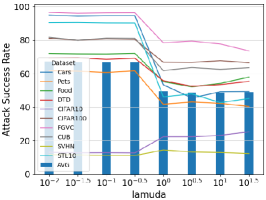
(a) Resnet101

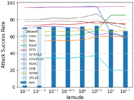
(b) Resnet50

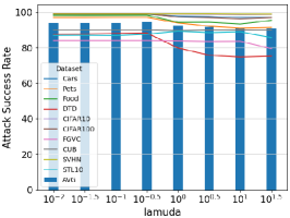
(c) ViT

Figure 9: The effect of the scale factor in L4A_fuse

C.2 Effect of using high-level loss

To study the effect of utilizing the high-level features, we choose Resnet50 pre-trained by SimCLRv2 as the target. In previous experiments, we found that the $L4A_{\text{fuse}}$ method performs best with $\lambda=1$. Thus, we fix it and add a new loss term summing over the lifting loss of the third, fourth and fifth layers, which is balanced by a hyperparameter $\mu$ (Note that we divided the Resnet50 into five blocks, meaning that it has five layers in total in our settings. Please refer to Appendix F.1 for more details about the model architecture). Finally the training loss of the experiments testing high-level layers can be formulated as follows:

$$\min_{\delta}L(f_{\theta},x,\delta)=-\mathbb{E}_{x\sim D_{p}}\bigg{[}\sum_{i=1}^{2}||f_{\theta}^{i}(x+\delta)||_{F}^{2}+\mu\sum_{j=3}^{5}||f_{\theta}^{j}(x+\delta)||_{F}^{2}\bigg{]},$$ (13)

We report the attack success rate (%) of using different $\mu$ against Resnet50 pre-trained by SimCLRv2. Note that C10 stands for CIFAR10, and C100 stands for CIFAR100. Results are shown in the Table 15.

Table 15: The attack success rate(%) of different $\mu$ against Resnet50 pretrained by SimCLRv2. Note that C10 stands for CIFAR10 and C100 stands for CIFAR100.

$\boldsymbol{\mathbf{\mu}}$	Cars	Pets	Food	DTD	FGVC	CUB	SVHN	C10	C100	STL10	AVG
0	96.00	59.80	65.00	77.93	95.02	85.05	69.39	64.41	76.29	37.54	72.64
0.01	95.32	56.99	63.60	76.06	94.93	83.31	69.65	67.30	77.55	37.76	72.25
0.1	95.00	56.06	62.02	75.00	95.32	82.21	66.76	70.36	77.86	35.28	71.59
1	95.16	56.55	62.11	74.95	95.20	82.27	67.15	69.20	78.47	35.75	71.68
10	96.17	55.16	62.08	77.82	95.26	83.52	66.48	67.37	77.56	33.39	71.48
100	61.78	42.71	59.86	70.05	86.68	66.26	63.43	86.99	64.92	21.78	62.44

As seen from the last column, the larger the weight of the loss of the high-level layers, the worse it performs. Moreover, when the loss of high-level layers overwhelms the low-level ones, the method suffers a significant performance drop (over 10%) in attack success rates. These results show that adding the high-level loss to the training loss bears negative effects.

C.3 Hyperparameters in the Uniform Gaussian Sampling.

We chose these hyperparameters as $\mu_{l}=0.4$, $\mu_{h}=0.6$, $\sigma_{l}=0.05$, $\sigma_{h}=0.1$ in the experiments. The reasons are as follows. For $\mu_{l}$ and $\mu_{h}$, we aim to make the mean $\mu$ drawn from $U(\mu_{l},\mu_{h})$ distributed around 0.5, since the input images are normalized to $[0,1]$. Thus we tried several configurations of $(\mu_{l},\mu_{h})$, such as (0.4, 0.6) and (0.45, 0.55), and found that (0.4, 0.6) performs best. For $\sigma_{l}$ and $\sigma_{h}$, we hope that most of the samples $n_{0}\sim N(\mu,\sigma)$ lie in $[0,1]$. Thus $\sigma\sim U(\sigma_{l},\sigma_{h})$ cannot be too large. We also tried some configurations of ($\sigma_{l}$, $\sigma_{h}$) and found that (0.05, 0.1) performs best.

Interestingly, the set (0.4, 0.6, 0.05, 0.10) generalizes well across the three models. Thus we did not tune these hyperparameters for each model but adopted a single configuration in Table 1, Table 2, and Table 3.

C.4 Pixel-level perturbations

To test the pixel-level perturbations, we add $\epsilon=0.05$ to the input images and then evaluate the performance on the three pre-trained models studied in the paper. Then we report the average attack success rate(%) on the ten datasets in Table 16, and detailed performance in Table 17. Note that SimR101, SimR101 and MAEViT stand for Resnet101 pretrained by SimCLRv2, Resnet50 pretrained by SimCLRv2 and ViT-base-16 pretrained by MAE, respectively.

Table 16: The average attack success of different methods against the three models. Note that C10 stands for CIFAR10 and C100 stands for CIFAR100.

methods	FFFno	FFFmean	FFFone	STD	SSP	ASV	UAP	EPGD	L4Abase	L4Afuse	L4Augs	Pixel
SimR101	48.55	44.22	40.26	42.63	40.75	46.65	43.86	59.34	66.89	71.90	72.20	12.97
SimR50	43.86	52.10	52.98	48.26	53.64	58.19	55.16	69.28	71.16	72.64	77.80	13.76
MAEViT	77.69	71.06	74.35	27.02	53.40	22.64	55.16	66.95	94.00	94.42	95.30	12.52

Table 17: The attack success rate(%) of the pixel-level attack on ten datasets. Note that C10 stands for CIFAR10 and C100 stands for CIFAR100.

ASR	Cars	Pets	Food	DTD	FGVC	CUB	SVHN	C10	C100	STL10	AVG
SimR101	10.42	9.70	12.15	29.36	23.79	21.25	2.61	2.21	15.46	2.75	12.97
SimR50	10.73	11.61	12.15	29.57	26.67	22.47	2.68	2.53	16.14	3.09	13.76
MAEViT	9.92	6.90	10.53	26.28	33.75	17.96	2.64	2.50	11.99	2.76	12.52

As we can see from the tables, the pixel-level perturbations have little effect on the predictions.

Appendix D Datasets

We evaluate the performance of pre-trained adversarial perturbations on the CIFAR100 and CIFAR10 [29], STL10 [8], Cars [28], Pets [49], Food [1], DTD [7], FGVC [38], CUB [57], SVHN [44]. We report the calibration (fine-grained or coarse-grained) and the accuracy on clean samples in Table 18.

Table 18: Calibration and ACC (%)

Dataset	Cars	Pets	Food	DTD	FGVC	CUB	SVHN	CIFAR10	CIFAR100	STL10
Calibration	fine	fine	fine	fine	fine	fine	fine	coarse	coarse	coarse
Resnet101 ACC	89.80	90.60	87.90	71.01	77.04	78.78	97.40	97.85	84.81	97.33
Resnet50 ACC	89.35	88.20	87.84	70.60	74.01	78.13	97.40	97.51	84.03	97.00
ViT ACC	90.03	93.48	89.60	73.60	67.16	82.32	97.38	98.10	88.03	97.20

Our datasets do not involve these issues.

Appendix E Visualisation of Perturbations

Figure 10: Visualization of pre-trained adversarial perturbations

Appendix F Implementations

F.1 Model architecture

To evaluate the effect of attacking different layers, we divide Resnet50, Resnet101 and ViT16 into 5 parts. Here we provide the mapping relationship from the original name to the five layers, respectively.

Table 19: Model architecture

Layers	layer1	layer2	layer3	layer4	layer5
Resnet50	net[0]	net[1]	net[2]	net[3]	net[4]
Resnet101	net[0]	net[1]	net[2]	net[3]	net[4]
ViT16	blocks[0]	blocks[1,2,3]	blocks[4,5,6]	blocks[7,8,9]	blocks[10,11]

F.2 Resources

We use one Nvidia GeForce RTX 2080 Ti for generating and evaluating PAPs.

References

- Bossard et al. [2014] Lukas Bossard, Matthieu Guillaumin, and Luc Van Gool. Food-101–mining discriminative components with random forests. In European Conference on Computer Vision (ECCV), pages 446–461, 2014.
- Brown et al. [2020] Tom Brown, Benjamin Mann, Nick Ryder, Melanie Subbiah, Jared D Kaplan, Prafulla Dhariwal, Arvind Neelakantan, Pranav Shyam, Girish Sastry, Amanda Askell, et al. Language models are few-shot learners. In Advances in Neural Information Processing Systems (NeurIPS), pages 1877–1901, 2020.
- Chen et al. [2020a] Tianlong Chen, Sijia Liu, Shiyu Chang, Yu Cheng, Lisa Amini, and Zhangyang Wang. Adversarial robustness: From self-supervised pre-training to fine-tuning. In Proceedings of the IEEE/CVF Conference on Computer Vision and Pattern Recognition (CVPR), pages 699–708, 2020a.
- Chen et al. [2020b] Ting Chen, Simon Kornblith, Mohammad Norouzi, and Geoffrey Hinton. A simple framework for contrastive learning of visual representations. In International Conference on Machine Learning (ICML), pages 1597–1607, 2020b.
- Chen et al. [2020c] Ting Chen, Simon Kornblith, Kevin Swersky, Mohammad Norouzi, and Geoffrey E Hinton. Big self-supervised models are strong semi-supervised learners. In Advances in Neural Information Processing Systems (NeurIPS), pages 22243–22255, 2020c.
- Chen and Ma [2021] Tong Chen and Zhan Ma. Towards robust neural image compression: Adversarial attack and model finetuning. arXiv preprint arXiv:2112.08691, 2021.
- Cimpoi et al. [2014] Mircea Cimpoi, Subhransu Maji, Iasonas Kokkinos, Sammy Mohamed, and Andrea Vedaldi. Describing textures in the wild. In Proceedings of the IEEE Conference on Computer Vision and Pattern Recognition (CVPR), pages 3606–3613, 2014.
- Coates et al. [2011] Adam Coates, Andrew Ng, and Honglak Lee. An analysis of single-layer networks in unsupervised feature learning. In Proceedings of the Fourteenth International Conference on Artificial Intelligence and Statistics (AISTATS), pages 215–223, 2011.
- Deng and Karam [2020] Yingpeng Deng and Lina J Karam. Universal adversarial attack via enhanced projected gradient descent. In IEEE International Conference on Image Processing (ICIP), pages 1241–1245, 2020.
- Dong et al. [2021] Xinshuai Dong, Anh Tuan Luu, Min Lin, Shuicheng Yan, and Hanwang Zhang. How should pre-trained language models be fine-tuned towards adversarial robustness? In Advances in Neural Information Processing Systems (NeurIPS), pages 4356–4369, 2021.
- Dong et al. [2018] Yinpeng Dong, Fangzhou Liao, Tianyu Pang, Hang Su, Jun Zhu, Xiaolin Hu, and Jianguo Li. Boosting adversarial attacks with momentum. In Proceedings of the IEEE Conference on Computer Vision and Pattern Recognition (CVPR), pages 9185–9193, 2018.
- Dong et al. [2019] Yinpeng Dong, Tianyu Pang, Hang Su, and Jun Zhu. Evading defenses to transferable adversarial examples by translation-invariant attacks. In Proceedings of the IEEE/CVF Conference on Computer Vision and Pattern Recognition (CVPR), pages 4312–4321, 2019.
- Fan et al. [2021] Lijie Fan, Sijia Liu, Pin-Yu Chen, Gaoyuan Zhang, and Chuang Gan. When does contrastive learning preserve adversarial robustness from pretraining to finetuning? In Advances in Neural Information Processing Systems (NeurIPS), pages 21480–21492, 2021.
- Gidaris et al. [2018] Spyros Gidaris, Praveer Singh, and Nikos Komodakis. Unsupervised representation learning by predicting image rotations. In International Conference on Learning Representations (ICLR), 2018.
- Goodfellow et al. [2015] Ian J Goodfellow, Jonathon Shlens, and Christian Szegedy. Explaining and harnessing adversarial examples. In International Conference on Learning Representations (ICLR), 2015.
- Guo et al. [2019] Yunhui Guo, Honghui Shi, Abhishek Kumar, Kristen Grauman, Tajana Rosing, and Rogerio Feris. Spottune: transfer learning through adaptive fine-tuning. In Proceedings of the IEEE/CVF Conference on Computer Vision and Pattern Recognition (CVPR), pages 4805–4814, 2019.
- Han et al. [2021] Xu Han, Zhengyan Zhang, Ning Ding, Yuxian Gu, Xiao Liu, Yuqi Huo, Jiezhong Qiu, Yuan Yao, Ao Zhang, Liang Zhang, et al. Pre-trained models: Past, present and future. AI Open, pages 225–250, 2021.
- He et al. [2016] Kaiming He, Xiangyu Zhang, Shaoqing Ren, and Jian Sun. Deep residual learning for image recognition. In Proceedings of the IEEE Conference on Computer Vision and Pattern Recognition (CVPR), pages 770–778, 2016.
- He et al. [2020a] Kaiming He, Haoqi Fan, Yuxin Wu, Saining Xie, and Ross Girshick. Momentum contrast for unsupervised visual representation learning. In Proceedings of the IEEE/CVF Conference on Computer Vision and Pattern Recognition (CVPR), pages 9729–9738, 2020a.
- He et al. [2020b] Kaiming He, Haoqi Fan, Yuxin Wu, Saining Xie, and Ross Girshick. Momentum contrast for unsupervised visual representation learning. In Proceedings of the IEEE/CVF Conference on Computer Vision and Pattern Recognition (CVPR), pages 9729–9738, 2020b.
- He et al. [2022] Kaiming He, Xinlei Chen, Saining Xie, Yanghao Li, Piotr Dollár, and Ross Girshick. Masked autoencoders are scalable vision learners. In Proceedings of the IEEE/CVF Conference on Computer Vision and Pattern Recognition (CVPR), pages 16000–16009, 2022.
- Inoue [2018] Hiroshi Inoue. Data augmentation by pairing samples for images classification. arXiv preprint arXiv:1801.02929, 2018.
- Ioffe and Szegedy [2015] Sergey Ioffe and Christian Szegedy. Batch normalization: Accelerating deep network training by reducing internal covariate shift. In International Conference on Machine Learning (ICML), pages 448–456, 2015.
- Jiang et al. [2020] Ziyu Jiang, Tianlong Chen, Ting Chen, and Zhangyang Wang. Robust pre-training by adversarial contrastive learning. In Advances in Neural Information Processing Systems (NeurIPS), pages 16199–16210, 2020.
- Kenton and Toutanova [2019] Jacob Devlin Ming-Wei Chang Kenton and Lee Kristina Toutanova. Bert: Pre-training of deep bidirectional transformers for language understanding. In Annual Conference of the North American Chapter of the Association for Computational Linguistics (NAACL), pages 4171–4186, 2019.
- Khosla et al. [2020] Prannay Khosla, Piotr Teterwak, Chen Wang, Aaron Sarna, Yonglong Tian, Phillip Isola, Aaron Maschinot, Ce Liu, and Dilip Krishnan. Supervised contrastive learning. In Advances in Neural Information Processing Systems (NeurIPS), pages 18661–18673, 2020.
- Khrulkov and Oseledets [2018] Valentin Khrulkov and Ivan Oseledets. Art of singular vectors and universal adversarial perturbations. In Proceedings of the IEEE Conference on Computer Vision and Pattern Recognition (CVPR), pages 8562–8570, 2018.
- Krause et al. [2013] Jonathan Krause, Jia Deng, Michael Stark, and Li Fei-Fei. Collecting a large-scale dataset of fine-grained cars. 2013.
- Krizhevsky et al. [2009] Alex Krizhevsky, Geoffrey Hinton, et al. Learning multiple layers of features from tiny images. 2009.
- Kumar et al. [2022] Ananya Kumar, Aditi Raghunathan, Robbie Jones, Tengyu Ma, and Percy Liang. Fine-tuning can distort pretrained features and underperform out-of-distribution. The International Conference on Learning Representations (ICLR), 2022.
- Kurakin et al. [2018] Alexey Kurakin, Ian J Goodfellow, and Samy Bengio. Adversarial examples in the physical world. In Artificial Intelligence Safety and Security, pages 99–112. 2018.
- Le-Khac et al. [2020] Phuc H Le-Khac, Graham Healy, and Alan F Smeaton. Contrastive representation learning: A framework and review. IEEE Access, pages 193907–193934, 2020.
- Liu et al. [2017] Yanpei Liu, Xinyun Chen, Chang Liu, and Dawn Song. Delving into transferable adversarial examples and black-box attacks. In International Conference on Learning Representations (ICLR), 2017.
- Liu et al. [2019] Yinhan Liu, Myle Ott, Naman Goyal, Jingfei Du, Mandar Joshi, Danqi Chen, Omer Levy, Mike Lewis, Luke Zettlemoyer, and Veselin Stoyanov. Roberta: A robustly optimized bert pretraining approach. arXiv preprint arXiv:1907.11692, 2019.
- Lu et al. [2020a] Yantao Lu, Yunhan Jia, Jianyu Wang, Bai Li, Weiheng Chai, Lawrence Carin, and Senem Velipasalar. Enhancing cross-task black-box transferability of adversarial examples with dispersion reduction. In Proceedings of the IEEE/CVF Conference on Computer Vision and Pattern Recognition (CVPR), pages 940–949, 2020a.
- Lu et al. [2020b] Yantao Lu, Yunhan Jia, Jianyu Wang, Bai Li, Weiheng Chai, Lawrence Carin, and Senem Velipasalar. Enhancing cross-task black-box transferability of adversarial examples with dispersion reduction. In Proceedings of the IEEE/CVF Conference on Computer Vision and Pattern Recognition (CVPR), pages 940–949, 2020b.
- Madry et al. [2018] Aleksander Madry, Aleksandar Makelov, Ludwig Schmidt, Dimitris Tsipras, and Adrian Vladu. Towards deep learning models resistant to adversarial attacks. In International Conference on Learning Representations (ICLR), 2018.
- Maji et al. [2013] Subhransu Maji, Esa Rahtu, Juho Kannala, Matthew Blaschko, and Andrea Vedaldi. Fine-grained visual classification of aircraft. arXiv preprint arXiv:1306.5151, 2013.
- Moosavi-Dezfooli et al. [2016] Seyed-Mohsen Moosavi-Dezfooli, Alhussein Fawzi, and Pascal Frossard. Deepfool: a simple and accurate method to fool deep neural networks. In Proceedings of the IEEE conference on computer vision and pattern recognition (CVPR), pages 2574–2582, 2016.
- Moosavi-Dezfooli et al. [2017] Seyed-Mohsen Moosavi-Dezfooli, Alhussein Fawzi, Omar Fawzi, and Pascal Frossard. Universal adversarial perturbations. In Proceedings of the IEEE Conference on Computer Vision and Pattern Recognition (CVPR), pages 1765–1773, 2017.
- Mopuri et al. [2017] Konda Reddy Mopuri, Utsav Garg, and R Venkatesh Babu. Fast feature fool: A data independent approach to universal adversarial perturbations. In British Machine Vision Conference (BMVC), 2017.
- Naseer et al. [2019] Muhammad Muzammal Naseer, Salman H Khan, Muhammad Haris Khan, Fahad Shahbaz Khan, and Fatih Porikli. Cross-domain transferability of adversarial perturbations. In Advances in Neural Information Processing Systems (NeurIPS), pages 12905–12915, 2019.
- Naseer et al. [2020] Muzammal Naseer, Salman Khan, Munawar Hayat, Fahad Shahbaz Khan, and Fatih Porikli. A self-supervised approach for adversarial robustness. In Proceedings of the IEEE/CVF Conference on Computer Vision and Pattern Recognition (CVPR), pages 262–271, 2020.
- Netzer et al. [2011] Yuval Netzer, Tao Wang, Adam Coates, Alessandro Bissacco, Bo Wu, and Andrew Y Ng. Reading digits in natural images with unsupervised feature learning. 2011.
- Noroozi and Favaro [2016] Mehdi Noroozi and Paolo Favaro. Unsupervised learning of visual representations by solving jigsaw puzzles. In European Conference on Computer Vision (ECCV), pages 69–84, 2016.
- Oquab et al. [2014] Maxime Oquab, Leon Bottou, Ivan Laptev, and Josef Sivic. Learning and transferring mid-level image representations using convolutional neural networks. In Proceedings of the IEEE Conference on Computer Vision and Pattern Recognition (CVPR), pages 1717–1724, 2014.
- Papernot et al. [2016] Nicolas Papernot, Patrick McDaniel, Somesh Jha, Matt Fredrikson, Z Berkay Celik, and Ananthram Swami. The limitations of deep learning in adversarial settings. In 2016 IEEE European Symposium on Security and Privacy (EuroS&P), pages 372–387, 2016.
- Park et al. [2020] Taesung Park, Alexei A Efros, Richard Zhang, and Jun-Yan Zhu. Contrastive learning for unpaired image-to-image translation. In European Conference on Computer Vision (ECCV), pages 319–345, 2020.
- Parkhi et al. [2012] Omkar M Parkhi, Andrea Vedaldi, Andrew Zisserman, and CV Jawahar. Cats and dogs. In Proceedings of the IEEE Conference on Computer Vision and Pattern Recognition (CVPR), pages 3498–3505, 2012.
- Qiu et al. [2020] Xipeng Qiu, Tianxiang Sun, Yige Xu, Yunfan Shao, Ning Dai, and Xuanjing Huang. Pre-trained models for natural language processing: A survey. Science China Technological Sciences, pages 1872–1897, 2020.
- Radford et al. [2021] Alec Radford, Jong Wook Kim, Chris Hallacy, Aditya Ramesh, Gabriel Goh, Sandhini Agarwal, Girish Sastry, Amanda Askell, Pamela Mishkin, Jack Clark, et al. Learning transferable visual models from natural language supervision. In International Conference on Machine Learning (ICML), pages 8748–8763, 2021.
- Russakovsky et al. [2015] Olga Russakovsky, Jia Deng, Hao Su, Jonathan Krause, Sanjeev Satheesh, Sean Ma, Zhiheng Huang, Andrej Karpathy, Aditya Khosla, Michael Bernstein, et al. Imagenet large scale visual recognition challenge. International journal of computer vision (IJCV), pages 211–252, 2015.
- Sai et al. [2020] Ananya B Sai, Akash Kumar Mohankumar, Siddhartha Arora, and Mitesh M Khapra. Improving dialog evaluation with a multi-reference adversarial dataset and large scale pretraining. Transactions of the Association for Computational Linguistics (TACL), pages 810–827, 2020.
- Szegedy et al. [2014] Christian Szegedy, Wojciech Zaremba, Ilya Sutskever, Joan Bruna, Dumitru Erhan, Ian Goodfellow, and Rob Fergus. Intriguing properties of neural networks. In International Conference on Learning Representations (ICLR), 2014.
- Trinh et al. [2019] Trieu H Trinh, Minh-Thang Luong, and Quoc V Le. Selfie: Self-supervised pretraining for image embedding. arXiv preprint arXiv:1906.02940, 2019.
- Vaswani et al. [2017] Ashish Vaswani, Noam Shazeer, Niki Parmar, Jakob Uszkoreit, Llion Jones, Aidan N Gomez, Łukasz Kaiser, and Illia Polosukhin. Attention is all you need. In Advances in neural information processing systems (NeurIPS), pages 6000–6010, 2017.
- Wah et al. [2011] Catherine Wah, Steve Branson, Peter Welinder, Pietro Perona, and Serge Belongie. The caltech-ucsd birds-200-2011 dataset. 2011.
- Xie et al. [2019] Cihang Xie, Zhishuai Zhang, Yuyin Zhou, Song Bai, Jianyu Wang, Zhou Ren, and Alan L Yuille. Improving transferability of adversarial examples with input diversity. In Proceedings of the IEEE/CVF Conference on Computer Vision and Pattern Recognition (CVPR), pages 2730–2739, 2019.
- Yan et al. [2020] Xueting Yan, Ishan Misra, Abhinav Gupta, Deepti Ghadiyaram, and Dhruv Mahajan. Clusterfit: Improving generalization of visual representations. In Proceedings of the IEEE/CVF Conference on Computer Vision and Pattern Recognition (CVPR), pages 6509–6518, 2020.
- Yang and Liu [2022] Zonghan Yang and Yang Liu. On robust prefix-tuning for text classification. In International Conference on Learning Representations (ICLR), 2022.
- Yosinski et al. [2014] Jason Yosinski, Jeff Clune, Yoshua Bengio, and Hod Lipson. How transferable are features in deep neural networks? In Advances in Neural Information Processing Systems (NeurIPS), pages 3320–3328, 2014.
- Yun et al. [2019] Sangdoo Yun, Dongyoon Han, Seong Joon Oh, Sanghyuk Chun, Junsuk Choe, and Youngjoon Yoo. Cutmix: Regularization strategy to train strong classifiers with localizable features. In Proceedings of the IEEE/CVF International Conference on Computer Vision (ICCV), pages 6023–6032, 2019.
- Zhang et al. [2021] Qilong Zhang, Xiaodan Li, Yuefeng Chen, Jingkuan Song, Lianli Gao, Yuan He, and Hui Xue. Beyond imagenet attack: Towards crafting adversarial examples for black-box domains. In International Conference on Learning Representations (ICLR), 2021.
- Zhang et al. [2016] Richard Zhang, Phillip Isola, and Alexei A Efros. Colorful image colorization. In European Conference on Computer Vision (ECCV), pages 649–666, 2016.