Queue replacement principle for corridor problems
with heterogeneous commuters

Abstract

This study investigates the theoretical properties of a departure time choice problem considering commuters’ heterogeneity with respect to the value of schedule delay in corridor networks. Specifically, we develop an analytical method to solve the dynamic system optimal (DSO) and dynamic user equilibrium (DUE) problems. To derive the DSO solution, we first demonstrate the bottleneck-based decomposition property, i.e., the DSO problem can be decomposed into multiple single bottleneck problems. Subsequently, we obtain the analytical solution by applying the theory of optimal transport to each decomposed problem and derive optimal congestion prices to achieve the DSO state. To derive the DUE solution, we prove the queue replacement principle (QRP) that the time-varying optimal congestion prices are equal to the queueing delay in the DUE state at every bottleneck. This principle enables us to derive a closed-form DUE solution based on the DSO solution. Moreover, as an application of the QRP, we prove that the equilibrium solution under various policies (e.g., on-ramp metering, on-ramp pricing, and its partial implementation) can be obtained analytically. Finally, we compare these equilibria with the DSO state.

1 Introduction

1.1 Background

The departure time choice problem proposed by Vickrey (1969) describes time-dependent traffic congestion as the dynamic user equilibrium (DUE) of commuters’ departure time choices. Many studies have analyzed the departure time choice problem in the classical framework with a single bottleneck and homogeneous commuters, and they have clarified theoretical properties, such as existence, uniqueness and the closed-form analytical solution (Vickrey, 1969; Hendrickson and Kocur, 1981; Smith, 1984; Daganzo, 1985; Newell, 1987; Arnott et al., 1993; Lindsey, 2004). These results provide important insights for designing traffic management policies, such as dynamic pricing and on-ramp metering (see Li et al. (2020) for a recent comprehensive review).

An important property of the single bottleneck model, assuming homogeneous commuters, is that when time-varying congestion prices mimicking the DUE queueing delay pattern are implemented, bottleneck congestion is eliminated without changing the arrival time at the destination of each commuter (Vickrey, 1969; Arnott, 1998). Such a dynamic pricing pattern leads the traffic state to a dynamic system optimal (DSO) state in which the total system cost is minimized (Hendrickson and Kocur, 1981; Arnott et al., 1993, 1994; Laih, 1994; Akamatsu et al., 2021). Therefore, the optimal pricing pattern can be obtained by observing the queueing delay pattern in the DUE state. Conversely, the queuing delay pattern in the DUE state can be obtained from the optimal pricing pattern in the DSO state (Iryo and Yoshii, 2007; Akamatsu et al., 2021). This means that the DUE flow pattern can be derived using the optimal pricing pattern in the DSO state.

Figure 1 illustrates this fact by comparing the DSO and DUE states. The horizontal axes in Figure 1(a)-(d) represent the arrival time $t\in\mathcal{T}$ at the destination of commuters, where $\mathcal{T}$ is the morning rush-hour. Figure 1(a) represents the cumulative arrival curve $A^{\mathrm{SO}}(\cdot)$ and cumulative departure curve $D^{\mathrm{SO}}(\cdot)$ for the DSO state. Because a queue is eliminated in the DSO state, if the free-flow travel time is ignored, the arrival curve $A^{\mathrm{SO}}(\cdot)$ is the same as the departure curve $D^{\mathrm{SO}}(\cdot)$. Figure 1(b) shows the optimal pricing pattern $p^{\mathrm{SO}}(t)$, which can be obtained as the optimal Lagrangian multiplier of a linear programming (LP) representing the DSO problem. Figure 1(d) shows that this optimal pricing pattern equals the queueing delay pattern $w^{\mathrm{UE}}(t)$ in the DUE state. In addtion, Figure 1(c) shows that the departure curve in the DUE state $D^{\mathrm{UE}}(\cdot)$ is the same as that in the DSO state. Based on $D^{\mathrm{UE}}(\cdot)$ and $w^{\mathrm{UE}}(t)$, the arrival curve in the DUE state $A^{\mathrm{UE}}(\cdot)$ can finally be obtained as shown in Figure 1(c).

We refer to this remarkable replaceability between the queueing delay and optimal pricing as the queue replacement principle (QRP).

Definition 1.1.

When the dynamic pricing pattern $\{p^{\mathrm{SO}}(t)\}_{t\in\mathcal{T}}$ in the DSO state is equal to the queueing delay pattern $\{w^{\mathrm{UE}}(t)\}_{t\in\mathcal{T}}$ in the DUE state, the QRP holds.

The QRP does not only contribute to obtaining the analytical solution, but it also clarifies the efficiency and equity of an optimal pricing scheme from the perspective of welfare analysis. In particula, the QRP shows that the travel costs of all commuters do not change with/without implementing optimal dynamic pricing. This means that the QRP is useful for designing an efficient and equitable traffic management scheme.

Considering these contributions of the QRP, it plays a pivotal role in analyzing the theoretical properties in more general settings, such as multiple-bottleneck networks and heterogeneous commuters. For this problem, Fu et al. (2022) investigated whether QRP holds for the departure time choice problem in corridor networks with multiple bottlenecks, and they demonstrated that QRP holds under certain assumptions. However, little is known about whether the QRP holds in the presence of heterogeneous commuters.

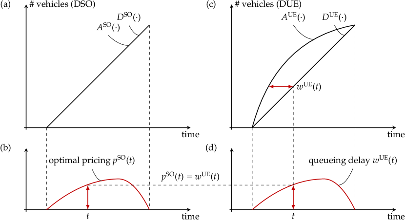
Figure 1: Queue replacement principle in a single bottleneck.

1.2 Purpose

This study proves that the QRP holds for corridor problems with heterogeneous commuters who have different values of schedule delay. We prove this QRP condition using the following two-step approach: we derive the analytical (I) DSO and (II) DUE solutions. In part (I), we first formulate the DSO problem as an LP. We demonstrate that the DSO solution is established according to the bottleneck-based decomposition property. This property enables us to decompose the DSO problem with multiple bottlenecks into independent single bottleneck problems, which are analytically solvable with the theory of optimal transport  (Rachev and Rüschendorf, 1998). From this analytical solution, we can derive the optimal congestion pricing pattern that achieves the DSO state.

In part (II), we investigate whether the queueing delay pattern is equivalent to the optimal pricing pattern. First, we formulate the DUE problem as a linear complementarity problem (LCP). Subsequently, we verify that the queueing delay pattern satisfies the physical requirements of a queue and that the associated DUE flow pattern can be constructed using this queuing delay pattern under a certain assumption which is related to the schedule delay cost function and nonnegative flow condition. From this approach, we find that there exists a DUE solution whose queueing delay pattern equals the optimal pricing pattern, i.e., we complete the proof of the QRP under the assumption.

This QRP implies a replaceability between commuters’ pricing and queueing costs at all bottlenecks. We clarify that this replaceability can independently hold at each bottleneck. Specifically, we focus on the case in which congestion pricing is only introduced for some bottlenecks. We demonstrate that the associated equilibrium can be derived by suitably replacing the queueing and pricing costs at each bottleneck. Furthermore, as an application of the obtained results, we show that such replaceability of commuters’ cost holds when on-ramp-based policies are implemented. Specifically, we consider equilibriums under on-ramp metering and pricing. We reveal that, at each on-ramp, the optimal pricing pattern equals the queueing pattern created by metering in equilibrium, just like the QRP. Finally, we investigate efficient policies by comparing equilibrium under the bottleneck-based and on-ramp-based policies.

1.3 Literature review

For multiple-bottleneck problems,  Kuwahara (1990) first analyzed the DUE problem in a two-tandem bottleneck network. Kuwahara (1990) showed a spatio-temporal sorting property of commuters’ arrival times. In Y-shaped networks with tandem bottlenecks,  Arnott et al. (1993) theoretically demonstrated a capacity-increasing paradox, and  Daniel et al. (2009) demonstrated a similar paradox in a laboratory setting.  Lago and Daganzo (2007) studied a similar problem with spillover and merging effects. However, applying their approach to analyze cases where an arbitrary number of bottlenecks exist is challenging because they employed the proof-by-cases method, as reported by Arnott and DePalma (2011). To overcome this limitation, Akamatsu et al. (2015) proposed a transparent formulation of the DUE problem in corridor networks with multiple bottlenecks. They introduced arrival-time-based variables (i.e., Lagrangian coordinate approach) that facilitate the analysis in corridor networks. Using the Lagrangian coordinate approach, Osawa et al. (2018) derived the solution to the DSO problem as part of the long-term location choice problem.  Fu et al. (2022) successfully derived the analytical solution to DUE problems in corridor networks with homogenous commuters.

For commuters’ heterogeneity, many studies focused on the single bottleneck problem. These studies are classified into two categories, depending on how heterogeneity is considered. One considered the heterogeneity of the preferred arrival time at the destination as analyzed in Hendrickson and Kocur (1981); Smith (1984); and Daganzo (1985). They proved the existence and uniqueness of the DUE solution and showed a regularity of the flow pattern, which is called the first-in-first-work principle. The other category considered the heterogeneity of the value of time; this includes Arnott et al. (1988, 1992, 1994); van den Berg and Verhoef (2011); Liu et al. (2015); and Takayama and Kuwahara (2017). They presented welfare analysis and showed that optimal policies can cause inequity in some cases.

In contrast to these studies, our study investigates the departure time choice problems in the corridor networks with commuters’ heterogeneity concerning the value of schedule delay. Our contributions are summarized as follows:

(1) Derivation of the analytical DSO solution:

This study constructs a systematic approach to solving the DSO problem. Specifically, by combining the bottleneck-based decomposition property and the theory of optimal transport, we show that the DSO problem can be solved by sequentially solving single bottleneck problems.

(2) Proof of the QRP:

This study investigates the DSO and DUE problems in corridor networks considering commuters’ heterogeneity in terms of the value of schedule delay. We successfully prove that the QRP holds under certain conditions.

(3) Derivation of the analytical DUE solution:

We derive the analytical DUE solution based on the DSO solution and QRP. Moreover, this contribution implies that the solution to an LCP (DUE problem), which is significantly difficult to solve analytically (Arnott and DePalma, 2011; Akamatsu et al., 2015), can be obtained from the solution to the LP (DSO problem). This is a theoretically/mathematically remarkable finding, representing a substantial advancement in the theory of dynamic traffic assignment problems.

(4) Derivation of the equilibria under various policies using the QRP:

As an application of Contributions (1)-(3), we show that the equilibria under on-ramp metering and on-ramp pricing can be derived using the QRP. This fact clarifies the theoretical relationships between bottleneck-based pricing and on-ramp-based policies. Moreover, we focus on cases in which policies are implemented at certain parts of the network and derive the associated equilibrium solution using the QRP. This means that the QRP enables us to analyze and characterize such an equilibrium state that is neither the pure DUE nor the DSO state.

1.4 Structure of this paper

The remainder of this paper is organized as follows: Section 2 introduces the network structure and the heterogeneity of commuters. Section 3 presents the formulation of the DSO problem and constructs the systematic approach for deriving its analytical solution. In Section 4, through the proof of the QRP, we derive the analytical solution to the DUE problem using the analytical DSO solution. Finally, Section 5 presents the application of the QRP. Section 6 concludes this paper. In this paper, all proofs of propositions are given in the appendix.

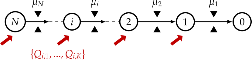
(a) Corridor network with $N$ origins and the single destination $0$.

(b) Schedule delay cost functions.

Figure 2: Network and schedule delay cost functions.

2 Model settings

2.1 Networks and commuters

We consider a freeway corridor network consisting of $N$ on-ramps (origin nodes) and a single off-ramp (destination node). These nodes are numbered sequentially from the destination node, denoted “$0$”, to the most distant origin node $N$ (Figure 2). The set of origin nodes is denoted by $\mathcal{N}\equiv\{1,2,\ldots,N\}$. The link connecting node $i$ to node $(i-1)$ is referred to as link $i$. Each link consists of a single bottleneck segment and free-flow segment. We refer to the bottleneck on link $i$ as bottleneck $i$.

Let $\mu_{i}$ be the capacity of bottleneck $i$. We also define $\overline{\mu}_{i}\equiv\mu_{i}-\mu_{(i+1)}$, where $\mu_{(N+1)}\equiv 0$. A queue is formed at each bottleneck when the inflow rate exceeds the bottleneck capacity. The queue dynamics are modeled by the standard point queue model along with the first-in-first-out (FIFO) principle. The free-flow travel time from origin (and bottleneck) $i\in\mathcal{N}$ to the destination is denoted by $d_{i}$.

From each origin $i$, $Q_{i}$ commuters enter the network and reach their destination during the morning rush-hour $\mathcal{T}$. Commuters are treated as a continuum, and the total mass $Q_{i}$ at each origin $i$ is a given constant. The commuters are also classified into a finite number $K$ of homogeneous groups with respect to the value of schedule delay. The index set of groups is $\mathcal{K}=\{1,2,\ldots,K\}$. The mass of commuters in group $k$ departing from origin $i$ is denoted by $Q_{i,k}$; therefore, $\sum_{k\in\mathcal{K}}Q_{i,k}=Q_{i}$. Commuters in group $k$ departing from origin $i$ are referred to as $(i,k)$-commuters.

The trip cost for each commuter is assumed to be additively separable into free-flow travel, queueing delay, and schedule delay costs. The schedule delay cost is defined as the difference between the actual and preferred arrival times at the destination. We assume that all commuters have the same preferred arrival time $t^{\mathrm{p}}=0$. The schedule delay cost for group $k$ commuters who arrive at the destination at time $t$ is represented by $c^{k}(t)$. We assume that $c^{k}(t)$ is represented by $\beta^{k}c(t)$, where $c(t)$ is a base schedule delay cost function with $c(t^{\mathrm{p}})=0$, which is assumed to be strictly quasi-convex and piecewise differentiable $\forall t\in\mathcal{T}$, as shown in Figure 2. In addtion, we assume $\mathrm{d}c(t)/\mathrm{d}t>-1$, $\forall t\in\mathcal{T}$ as in Daganzo (1985); Lindsey (2004). $\beta^{k}\in(0,1]$ is a parameter representing the heterogeneity of commuters with $\beta^{K}<...<\beta^{1}=1$. We also let $\overline{\beta}^{k}\equiv\beta^{k}-\beta^{(k+1)}$, where $\beta^{(K+1)}\equiv 0$.

Because $c(t)$ is strictly convex, for a given time length $T$, we can define $t^{-}(T)$ as the unique solution to the equation $c(t)=c(t+T)$. We define $t^{+}(T)$ as $t^{+}(T)=t^{-}(T)+T$. The base schedule delay cost at $t^{-}(T)$ (and $t^{+}(T)$) is denoted by $\overline{c}(T)$ (i.e., $\overline{c}(T)=c(t^{-}(T))=c(t^{+}(T))$). We also define time set $\Gamma(T)$ as

$$\Gamma(T)\equiv[t^{-}(T),t^{+}(T)],$$ (1)

where $\Gamma(T)$ is uniquely determined for $T$ (see Figure 3).

Figure 3: $T$ and $\Gamma(T)$, in relation to $c(t)$.

2.2 Formulation in a Lagrangian-like coordinate system

We primarily describe traffic variables in a Lagrangian-like coordinate system (Kuwahara and Akamatsu, 1993; Akamatsu et al., 2015, 2021). In this system, variables are expressed in association with the arrival time at the destination, and not at the origin or bottleneck. Such an expression is suitable for considering the ex-post travel time of each commuter during their trip. Therefore, we can easily trace the time-space paths of commuters.

Several variables are introduced for the expression of within-day dynamic traffic flow in this system. We define $\tau_{i}(t)$ and $\sigma_{i}(t)$ as the arrival and departure times at bottleneck $i\in\mathcal{N}$, respectively, for commuters whose destination arrival time is $t$. The queuing delay at bottleneck $i$ for the commuters arriving at time $t$ at the destination is denoted by $w_{i}(t)$. These variables satisfy the following relationships:

$$\tau_{i}(t)=t-\sum_{j;j\leq i}w_{j}(t)-d_{i} \forall i\in\mathcal{N},\quad\forall t\in\mathcal{T},$$ (2)

$$\sigma_{i}(t)=t-\sum_{j;j<i}w_{j}(t)-d_{(i-1)} \forall i\in\mathcal{N},\quad\forall t\in\mathcal{T}.$$ (3)

Note that $\tau_{i}(t)$ must satisfy the following relationship:

$$\cfrac{\mathrm{d}\tau_{i}(t)}{\mathrm{d}t}\equiv\dot{\tau}_{i}(t)>0, \forall i\in\mathcal{N},\quad\forall t\in\mathcal{T},$$ (4)

where an overdot denotes the derivative of the variable with respect to the destination arrival time $t$. This condition guarantees the Lipschitz continuity of cumulative arrival flows, which means that the traffic flow is physically consistent (Akamatsu et al., 2015; Fu et al., 2022; Sakai et al., 2022). Hereafter, we refer to Condition (4) as the consistency condition.

2.3 Physical conditions for a dynamic traffic flow

We formulate physical conditions for dynamic traffic flow. First, the inflow from each origin must satisfy the following demand conservation condition:

$$\int_{\mathcal{T}}q_{i,k}(t)\mathrm{d}t=Q_{i,k} \forall k\in\mathcal{K},\quad\forall i\in\mathcal{N},$$ (5)

where $q_{i,k}(t)\geq 0$ is the inflow rate to the network of $(i,k)$-commuters whose destination arrival time is $t$.

Subsequently, we describe the queueing congestion at each bottleneck. Let $x_{i}(t)$ be the departure flow rate at link $i\in\mathcal{N}$. Then, the queueing condition is described as the following complementarity condition:

$$\begin{dcases}x_{i}(\sigma_{i}(t))=\mu_{i}\quad&\mathrm{if}\quad w_{i}(t)>0\\ x_{i}(\sigma_{i}(t))\leq\mu_{i}\quad&\mathrm{if}\quad w_{i}(t)=0\end{dcases} \quad\forall k\in\mathcal{K},\quad\forall i\in\mathcal{N},\quad\forall t\in\mathcal{T}.$$ (6)

Thirdly, we formulate the flow conservation condition at each node. This condition requires that for each time, the inflow rate to a node should equal the outflow rate from the node. Mathematically, this is described as

$$\cfrac{\mathrm{d}D_{(i+1)}(\sigma_{(i+1)}(t))}{\mathrm{d}t}+\sum_{k\in\mathcal{K}}q_{i,k}(t)=\cfrac{\mathrm{d}A_{i}(\tau_{i}(t))}{\mathrm{d}t} \quad\forall i\in\mathcal{N},\quad\forall t\in\mathcal{T}.$$ (7)

Here, the FIFO principle is expressed as

$$A_{i}(\tau_{i}(t))=D_{i}(\sigma_{i}(t)) \quad\forall i\in\mathcal{N},\quad\forall t\in\mathcal{T}.$$ (8)

Substituting this into the flow conservation condition, we obtain

$$x_{(i+1)}(\sigma_{(i+1)}(t))\dot{\sigma}_{(i+1)}(t)+\sum_{k\in\mathcal{K}}q_{i,k}(t)=x_{i}(\sigma_{i}(t))\dot{\sigma}_{i}(t) \quad\forall i\in\mathcal{N},\quad\forall t\in\mathcal{T}.$$ (9)

We have the following equation by recursively applying this toward descendants of each node $i$:

$$\sum_{j;j\geq i}\sum_{k\in\mathcal{K}}q_{i,k}(t)=x_{i}(\sigma_{i}(t))\dot{\sigma}_{i}(t) \quad\forall i\in\mathcal{N},\quad\forall t\in\mathcal{T}.$$ (10)

Substituting the flow conservation condition (10) into (6), we can describe the queueing condition by using the variable $q_{i,k}(t)$, as follows:

$$\begin{dcases}\sum_{j;j\geq i}\sum_{k\in\mathcal{K}}q_{j,k}(t)=\mu_{i}\dot{\sigma}_{i}(t)\quad&\mathrm{if}\quad w_{i}(t)>0\\ \sum_{j;j\geq i}\sum_{k\in\mathcal{K}}q_{j,k}(t)\leq\mu_{i}\dot{\sigma}_{i}(t)\quad&\mathrm{if}\quad w_{i}(t)=0\end{dcases} \forall i\in\mathcal{N},\quad\forall t\in\mathcal{T}.$$ (11)

3 Dynamic system optimal problem

In this section, an analytical solution to the DSO problem is derived. Section 3.1 formulates the DSO problem as an LP. Section 3.2 derives the aggregated DSO flow by decomposing the problem into sub-problems with respect to bottlenecks under a certain assumption. Section 3.3 presents the approach for deriving the disaggregated DSO flow from the aggregate arrival DSO flow by applying the theory of optimal transport (Rachev and Rüschendorf, 1998).

3.1 Formulation of the DSO problem

We define a DSO state as a state in which the total transport cost is minimized without queues, i.e., congestion externalities are completely eliminated. Mathematically, the DSO problem is formulated as the following LP (Osawa et al., 2018; Fu et al., 2022):

[DSO]

$$\min_{q_{i,k}(t)\geq\bm{0}}.\quad \sum_{i\in\mathcal{N}}\sum_{k\in\mathcal{K}}\int_{\mathcal{T}}\left(\beta^{k}c(t)+d_{i}\right)q_{i,k}(t)\mathrm{d}t$$ (12)

s.t. $$\int_{\mathcal{T}}q_{i,k}(t)\mathrm{d}t=Q_{i,k} \forall k\in\mathcal{K},\quad\forall i\in\mathcal{N},$$ (13)

$$\sum_{j;j\geq i}q_{j}(t)\leq\mu_{i} \forall i\in\mathcal{N},\quad\forall t\in\mathcal{T},$$ (14)

where $q_{i}(t)$ is the aggregated destination arrival flow at $t$ of commuters departing from origin $i$: $q_{i}(t)\equiv\sum_{k\in\mathcal{K}}q_{i,k}(t)$. The objective function is the total schedule delay costs of all commuters. The first constraint is the flow conservation condition equivalent to (5). The second constraint is the queueing condition equivalent to (11) when there are no queues.

The optimality conditions of [DSO] are given as follows (Luenberger, 1997; Akamatsu et al., 2021):

$$0\leq q^{\mathrm{SO}}_{i,k}(t)\perp\left\{\beta^{k}c(t)+\sum_{j;j\leq i}p^{\mathrm{SO}}_{j}(t)+d_{i}-\rho^{\mathrm{SO}}_{i,k}\right\}\geq 0 \forall k\in\mathcal{K},\quad\forall i\in\mathcal{N},\quad\forall t\in\mathcal{T},$$ (15)

$$0\leq p^{\mathrm{SO}}_{i}(t)\perp\left\{\mu_{i}-\sum_{j;j\geq i}q^{\mathrm{SO}}_{j}(t)\right\}\geq 0 \forall i\in\mathcal{N},\quad\forall t\in\mathcal{T},$$ (16)

$$0\leq\rho^{\mathrm{SO}}_{i,k}\perp\left\{\int_{\mathcal{T}}q^{\mathrm{SO}}_{i,k}(t)\mathrm{d}t-Q_{i,k}\right\}\geq 0 \forall k\in\mathcal{K},\quad\forall i\in\mathcal{N},$$ (17)

where $\rho_{i,k}$ and $p_{i}(t)$ are the Lagrange multipliers for Constraints (13) and (14), respectively. The superscript SO indicates that the variables are the optimal solution to [DSO].

It is worth noting that we can interpret these optimality conditions as equilibrium conditions under an optimal dynamic congestion pricing scheme (Arnott et al., 1990; Laih, 1994; Lindsey et al., 2012; Chen et al., 2015). This indicates that $\{p^{\mathrm{SO}}_{i}(t)\}_{i\in\mathcal{N}}$ can be regarded as an optimal pricing pattern, and $\rho^{\mathrm{SO}}_{i,k}=\tilde{\rho}^{\mathrm{SO}}_{i,k}-d_{i}$ can be regarded as the equilibrium commuting cost of $(i,k)$-commuters. Eq. 15 can then be interpreted as the equilibrium condition for commuters’ departure time choice condition under the pricing scheme. This interpretation from the perspective of equilibrium conditions helps us obtain the analytical solution to [DSO].

3.2 Aggregated DSO flow pattern

In the following sections, we present a systematic approach to obtain an analytical solution to the DSO problem. This section obtains the aggregated DSO flow pattern and shows the decomposition property of [DSO] as a first step of this approach.

As Fu et al. (2022) noted, the DSO flow pattern in the corridor problem may have arbitrariness. To exclude these cases and clarify the analysis approach, we introduce the following assumptions regarding flow and pricing patterns in the DSO state.

Assumption 3.1.

For all bottleneck $i\in\mathcal{N}$, the following relationship is satisfied:

$$p^{\mathrm{SO}}_{i}(t)>0\quad\Leftrightarrow\quad q^{\mathrm{SO}}_{i}(t)>0 \forall i\in\mathcal{N},\quad\forall t\in\mathcal{T}.$$ (18)

The time window $\mathcal{T}^{\mathrm{SO}}_{i}\equiv\mathrm{supp}\left(p^{\mathrm{SO}}_{i}(t)\right)=\mathrm{supp}\left(q^{\mathrm{SO}}_{i}(t)\right)$ is convex for all $i\in\mathcal{N}$.

This assumption implies that all commuters experience optimal congestion prices, which are non-zero, at all their passing bottlenecks. This assumption also implies that the network has no false bottlenecks, whose optimal prices are always zero. In the corridor network with false bottlenecks, the DSO flow pattern has arbitrariness (Fu et al., 2022). Using this assumption, we can exclude the case where the optimal flow patterns of the closed-form solution have arbitrariness, which causes unnecessary complications for the analysis.

Assumption 3.1 may seem restrictive, but it does not limit the situations that can be analyzed. A network that satisfies Assumption 3.1 can be constructed from any corridor network with arbitrary capacity patterns by applying the algorithm proposed by Fu et al. (2022). The algorithm detects false bottlenecks, whose optimal prices are always zero, and reduces the false bottlenecks and corresponding origins by aggregating travel demands from the upstream and downstream origins of each false bottleneck (see Fu et al. 2022, Appendix B). Note that, in this reduced network, $\mu_{i}-\mu_{(i+1)}>0$, $\forall i\in\mathcal{N}\setminus\{N\}$ is the necessary condition of Assumption 3.1. If $\mu_{i}-\mu_{(i+1)}\leq 0$, the bottleneck capacity constraint condition (14) and the non-false bottleneck condition cannot be achieved simultaneously.

Under this assumption, we have the following lemma:

Lemma 3.1.

Suppose that Assumption 3.1 holds. The arrival time window of $i$-commuters, who depart from origin $i\in\mathcal{N}\setminus\{N\}$, is included in that of $(i+1)$-commuters in the DSO state:

$$\mathcal{T}^{\mathrm{SO}}_{i}\subset\mathcal{T}^{\mathrm{SO}}_{(i+1)} \forall i\in\mathcal{N}\setminus\{N\}.$$ (19)

This lemma shows the spatial sorting property of the DSO flow pattern (Fu et al., 2022). Specifically, the first commuters to depart from origin $i$ arrive at the destination later than the first commuters to depart from the immediate upstream origin $i+1$; the last commuters to depart from origin $i$ arrive earlier than the last commuters to depart from origin $i+1$; and the arrival time windows have nested structures.

Using this property, we obtain the aggregated DSO flow pattern $\{q^{\mathrm{SO}}_{i}(t)\}$, as follows:

Lemma 3.2.

Suppose that Assumption 3.1 holds, the aggregated DSO flow is given as:

$$q^{\mathrm{SO}}_{i}(t) =\begin{dcases}\overline{\mu}_{i}\quad&\mathrm{if}\quad t\in\mathcal{T}^{\mathrm{SO}}_{i}\\ 0\quad&\mathrm{otherwise}\end{dcases} \forall i\in\mathcal{N},$$ (20)

where $\overline{\mu}_{i}=\mu_{i}-\mu_{(i+1)}$ and $\mu_{(N+1)}=0$. The length of the arrival time window $T^{\mathrm{SO}}_{i}\equiv|\mathcal{T}^{\mathrm{SO}}_{i}|$ is determined as $T^{\mathrm{SO}}_{i}=\sum_{k\in\mathcal{K}}Q_{i,k}/\overline{\mu}_{i}$.

This lemma shows that the aggregated DSO flow pattern becomes an all-or-nothing pattern. The aggregated inflow rate $q^{\mathrm{SO}}_{i}(t)$ equals the difference in the capacities between the immediate downstream and upstream bottlenecks during $\mathcal{T}^{\mathrm{SO}}_{i}$; otherwise, the inflow rate becomes zero. Figure 4 (a) shows the aggregated DSO flow pattern with $N=3$. We find that the spatial sorting property makes the aggregated DSO flow pattern as a staircase. Figure 4 also illustrates that the time window $\mathcal{T}^{\mathrm{SO}}_{i}$ is determined by $\Gamma(T^{\mathrm{SO}}_{i})$, where $\Gamma(\cdot)$ is defined by Eq. 1. This fact is derived from Lemma 3.6, which will be discussed later. From Lemma 3.6, the first and last commuters from origin $i$ to arrive at the destination are both in group $K$. Based on the optimality condition (15) and Assumption 3.1, we find $\beta^{K}c(\min.\{\mathcal{T}^{\mathrm{SO}}_{i}\})=\beta^{K}c(\max.\{\mathcal{T}^{\mathrm{SO}}_{i}\})$ for all $i\in\mathcal{N}$. Hence, the time window $\mathcal{T}^{\mathrm{SO}}_{i}$ is determined by $\Gamma(T^{\mathrm{SO}}_{i})$ as shown in Figure 4(a) and (b).

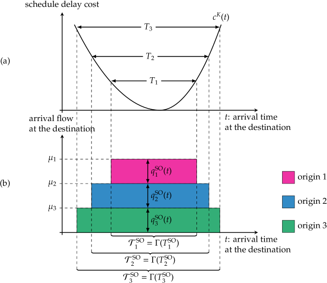
Figure 4: Aggregated DSO arrival flow pattern at the destination with the spatial-sorting property.

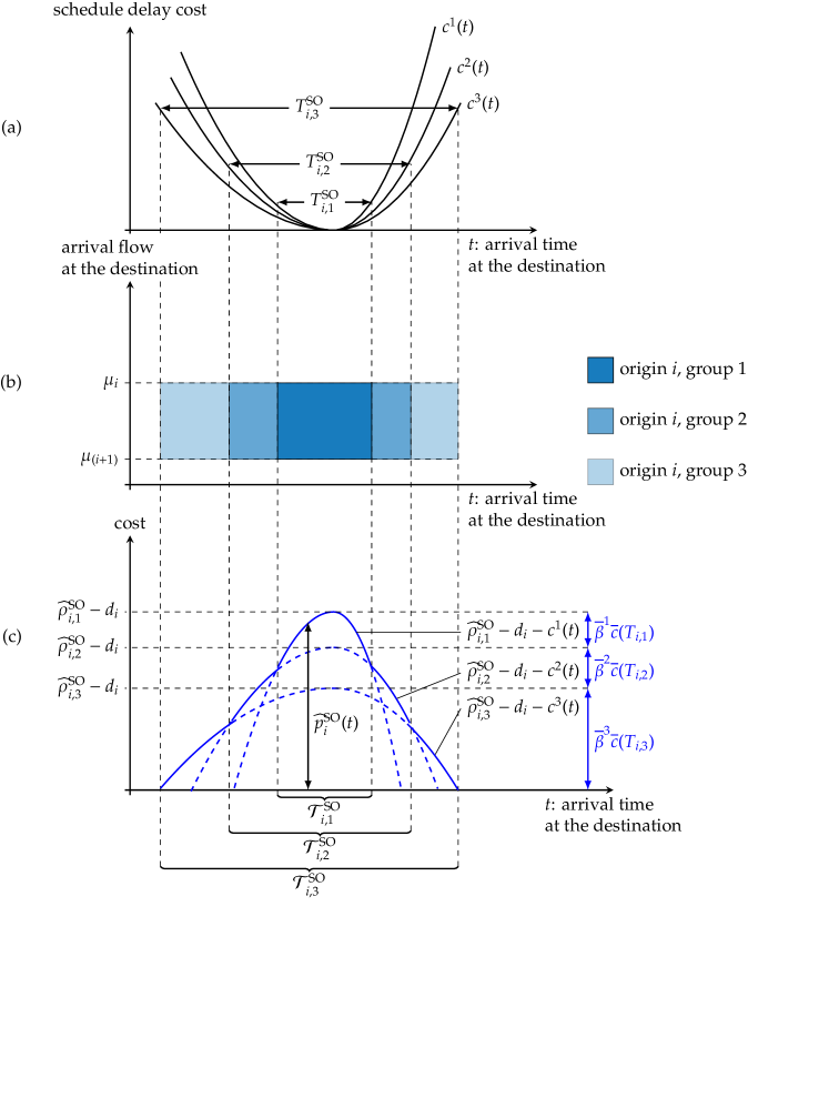
Figure 5: Disaggregated DSO arrival flow pattern at the destination with the temporal-sorting property.

Interestingly, Lemma 3.2 is more than a simple contribution toward clarifying the aggregated DSO flow pattern. This enables us to decompose the DSO problem in a corridor network into bottleneck-based sub-problems, which are useful for obtaining the disaggregated DSO flow pattern, i.e., inflow rate of commuters in each group. The lemma eliminates the interaction of bottlenecks in Constraint (14), and Constraint (14) can be independently rewritten as follows:

$$\sum_{k\in\mathcal{K}}q_{i,k}(t)=\overline{\mu}_{i} \forall i\in\mathcal{N},\quad\forall t\in\mathcal{T}^{\mathrm{SO}}_{i}.$$ (21)

Because the RHS of Eq. 21 is constant, this form implies the separation of Eq. 14 by each bottleneck $i$. Additionally, the objective function of [DSO] can also be separated by each origin (bottleneck) $i$, and the demand conservation constraint (13) is already independent at each origin $i$. Consequently, we find that the objective function and all constraints of [DSO] can be separated by each origin (bottleneck) $i$. This means we can independently consider each bottleneck-based sub-problem without considering the other sub-problems. Hence, for obtaining the disaggregated DSO flow pattern, we do not have to deal with complex spatial interactions between multiple bottlenecks; we solve the sub-problem, which has the same mathematical structure as a single bottleneck problem. This is summarized in the following lemma:

Lemma 3.3 (Decomposition Property).

Suppose that Assumption 3.1 holds. Then, the solution to [DSO] can be obtained by solving the following sub-problems [DSO-Sub$(i)$] for every bottleneck $i\in\mathcal{N}$:

[DSO-Sub$$(i)$$]

$$\min_{\{q_{i,k}(t)\}_{k\in\mathcal{K},t\in\mathcal{T}}\geq\bm{0}}.\quad \sum_{k\in\mathcal{K}}\int_{\mathcal{T}^{\mathrm{SO}}_{i}}\left(\beta^{k}c(t)+d_{i}\right)q_{i,k}(t)\mathrm{d}t$$ (22)

s.t. $$\int_{\mathcal{T}^{\mathrm{SO}}_{i}}q_{i,k}(t)\mathrm{d}t=Q_{i,k} \forall k\in\mathcal{K},$$ (23)

$$\sum_{k\in\mathcal{K}}q_{i,k}(t)=\overline{\mu}_{i} \forall t\in\mathcal{T}^{\mathrm{SO}}_{i}.$$ (24)

The optimality conditions of [DSO-Sub$(i)$] are given as follows:

$$0\leq q^{\mathrm{SO}}_{i,k}(t)\perp\left\{\beta^{k}c(t)+\widehat{p}^{\mathrm{SO}}_{i}(t)+d_{i}-\widehat{\rho}^{\mathrm{SO}}_{i,k}\right\}\geq 0 \forall k\in\mathcal{K},\quad\forall t\in\mathcal{T},$$ (25)

$$\overline{\mu}_{i}-\sum_{k\in\mathcal{K}}q^{\mathrm{SO}}_{i,k}(t)=0 \forall t\in\mathcal{T},$$ (26)

$$\int_{\mathcal{T}}q^{\mathrm{SO}}_{i,k}(t)\mathrm{d}t-Q_{i,k}=0 \forall k\in\mathcal{K},$$ (27)

where $\widehat{\rho}_{i,k}$ and $\widehat{p}_{i}(t)$ are the Lagrange multipliers for constraints (23) and (24), respectively.

3.3 Disaggregated DSO flow pattern

The remainder of our approach is to obtain the disaggregated DSO flow pattern by analytically solving the sub-problems. We remember that this sub-problem [DSO-Sub(i)] has the same structure as the single bottleneck problem. Note that total free-flow travel cost is constant and does not affect the optimal flow pattern. As discussed in Akamatsu et al. (2021), the mathematical structure of the single bottleneck problem is the same as that of the optimal transport problem (Rachev and Rüschendorf, 1998), which is well known as Hitchcock’s transportation problem in operations research and transportation fields. Moreover, Akamatsu et al. (2021) demonstrated that the analytical solution to the single bottleneck problem could be derived using the theory of optimal transport when the transport cost function, $c^{k}(t)$ in Eq. (22), satisfies the submodularity property. Therefore, it is sufficient to confirm that the schedule delay cost function satisfies that property.

We first introduce the definition of the submodularity property:

Definition 3.1.

Function $c:\mathbb{R}^{2}\rightarrow\mathbb{R}$ is submodular if, and only if,

$$c(x,y)+c(x^{\prime},y^{\prime})\leq c(x,y^{\prime})+c(x^{\prime},y)\quad\forall x\leq x^{\prime},y\leq y^{\prime}.$$ (28)

If the inequality in Eq. 28 strictly holds for $x^{\prime}<x$, and $y<y^{\prime}$, $c$ is called a strict submodular function. In addition, if the inequality Eq. 28 holds in the opposite direction, then function $c$ is supermodular.

In our sub-problem [DSO-Sub$(i)$], the schedule delay cost function $\beta^{k}c(t)$ is submodular and supermodular in $t\geq 0$ and $t<0$, respectively:

Lemma 3.4.

The schedule delay cost function $\beta^{k}c(t)$ is the submodular function for all $t\geq 0$:

$$\beta^{k}c(t)+\beta^{k+1}c(t^{\prime})<\beta^{k+1}c(t)+\beta^{k}c(t^{\prime}) \forall k\in\mathcal{K},\quad\forall t^{\prime}>t.$$ (29)

Lemma 3.5.

The schedule delay cost function $\beta^{k}c(t)$ is the supermodular function for all $t<0$:

$$\beta^{k}c(t)+\beta^{k+1}c(t^{\prime})>\beta^{k+1}c(t)+\beta^{k}c(t^{\prime}) \forall k\in\mathcal{K},\quad\forall t^{\prime}>t.$$ (30)

A detailed discussion was given by Akamatsu et al. (2021), but here we remark that the submodularity (supermodularity) of $c^{k}(t)$ prioritizes all groups. Specifically, in the optimal solution, all $(i,k)$-commuters arrive at the destination closer to the preferred arrival time than the $(i,k+1)$-commuters. In other words, for all origins $i\in\mathcal{N}$, the arrival time window of the $(i,k+1)$-commuters includes that of the $(i,k)$-commuters. Based on this temporal sorting property and the optimality condition of [DSO-Sub$(i)$], we obtain the analytical solution to [DSO-Sub$(i)$] as follows:

Lemma 3.6 ( Akamatsu et al. (2021)).

The following $\{\bm{q}^{\mathrm{SO}}(t)\}_{t\in\mathcal{T}}$, $\widehat{\bm{\rho}}^{\mathrm{SO}}$, and $\{\widehat{\bm{p}}^{\mathrm{SO}}(t)\}_{t\in\mathcal{T}}$ are solutions to [DSO-Sub$(i)$]:

$$q^{\mathrm{SO}}_{i,k}(t)=\begin{dcases}\overline{\mu}_{i}&\mathrm{if}\quad\forall t\in\mathcal{T}^{\mathrm{SO}}_{i,k}\setminus\mathcal{T}^{\mathrm{SO}}_{i,(k-1)}\\ 0&\mathrm{otherwise}\end{dcases} \forall k\in\mathcal{K},$$ (31)

$$\widehat{\rho}^{\mathrm{SO}}_{i,k}=\sum_{l;l\geq k}\overline{\beta}^{l}\overline{c}(T^{\mathrm{SO}}_{i,k})+d_{i} \forall k\in\mathcal{K},$$ (32)

$$\widehat{p}^{\mathrm{SO}}_{i}(t)=\widehat{\rho}^{\mathrm{SO}}_{i,k}-\beta^{k}c(t) \forall t\in\mathcal{T}^{\mathrm{SO}}_{i,k}\setminus\mathcal{T}^{\mathrm{SO}}_{i,(k-1)},$$ (33)

where $\mathcal{T}^{\mathrm{SO}}_{i,k}=\Gamma(T^{\mathrm{SO}}_{i,k})$ and $T^{\mathrm{SO}}_{i,k}=\sum_{l;l\leq k}Q_{i,l}/\overline{\mu}_{i}$. Note that $\overline{\beta}^{k}=\beta^{k}-\beta^{(k+1)}$ and $\beta^{(K+1)}=0$.

Figure 5 illustrates the solution to the sub-problem [DSO-Sub$(i)$] with $K=3$. Figure 5 (b) represents the disaggregated DSO flow pattern $\{\bm{q}^{\mathrm{SO}}(t)\}_{t\in\mathcal{T}}$ with the temporal sorting property that the arrival time window of the $(i,k+1)$-commuters includes that of the $(i,k)$-commuters. The arrival time windows are determined by the schedule delay cost functions as shown in Figure 5 (a) and (b). Moreover, Figure 5 (c) illustrates the optimal Lagrangian multipliers.

Combining these analytical solutions to the sub-problems, we immediately construct the complete DSO flow pattern. Moreover, the analytical solutions to the sub-problems enable us to derive the optimal Lagrangian multipliers of [DSO-LP], which represent the congestion price and equilibrium commuting cost. Specifically, based on the optimality condition of [DSO-LP], we find that $\rho^{\mathrm{SO}}_{i,k}=\widehat{\rho}^{\mathrm{SO}}_{i,k}$ and $p^{\mathrm{SO}}_{i}(t)=\min.\{0,\ \widehat{p}^{\mathrm{SO}}_{i}(t)-\widehat{p}^{\mathrm{SO}}_{(i-1)}(t)\}$. This is summarized as follows:

Proposition 3.1 (Solution to the DSO Problem).

If Assumption 3.1 holds, then, the following $\{\bm{q}^{\mathrm{SO}}(t)\}_{t\in\mathcal{T}}$ is a solution to [DSO], and the following $\bm{\rho}^{\mathrm{SO}}$ and $\{\bm{p}^{\mathrm{SO}}(t)\}_{t\in\mathcal{T}}$ are optimal Lagrangian multipliers of [DSO]:

$$q^{\mathrm{SO}}_{i,k}(t) =\begin{dcases}\overline{\mu}_{i}&\mathrm{if}\ t\in\mathcal{T}^{\mathrm{SO}}_{i,k}\setminus\mathcal{T}^{\mathrm{SO}}_{i,(k-1)}\\ 0&\mathrm{otherwise}\end{dcases} \forall k\in\mathcal{K},\quad\forall i\in\mathcal{N},$$ (34)

$$\rho^{\mathrm{SO}}_{i,k} =\sum_{l;l\geq k}\overline{\beta}^{l}\overline{c}(T^{\mathrm{SO}}_{i,k})+d_{i} \forall k\in\mathcal{K},\quad\forall i\in\mathcal{N},$$ (35)

$$p^{\mathrm{SO}}_{i}(t) =\begin{dcases}\rho^{\mathrm{SO}}_{i,k}-\beta^{k}c(t)-\sum_{j;j<i}p^{\mathrm{SO}}_{j}(t)&\mathrm{if}\ t\in\mathcal{T}^{\mathrm{SO}}_{i,k}\setminus\mathcal{T}^{\mathrm{SO}}_{i,(k-1)}\\ 0&\mathrm{otherwise}\end{dcases} \forall i\in\mathcal{N}.$$ (36)

Figure 6 illustrates the solution to the DSO problem for the case of $(N,K)=(2,2)$. Figure 6 (a) depicts the relationship between the schedule delay cost function and the arrival time window of the commuters. Figure 6 (b) and (c) illustrates the DSO arrival flow pattern $\{\bm{q}^{\mathrm{SO}}\}_{t\in\mathcal{T}}$ and the optimal Lagrangian multipliers $\{\bm{p}^{\mathrm{SO}}(t)\}_{t\in\mathcal{T}}$, $\bm{\rho}^{\mathrm{SO}}$, respectively. We find that $\{\bm{q}^{\mathrm{SO}}\}_{t\in\mathcal{T}}$, $\{\bm{p}^{\mathrm{SO}}(t)\}_{t\in\mathcal{T}}$, and $\bm{\rho}^{\mathrm{SO}}$ can be constructed by combining the solutions to the sub-problems.

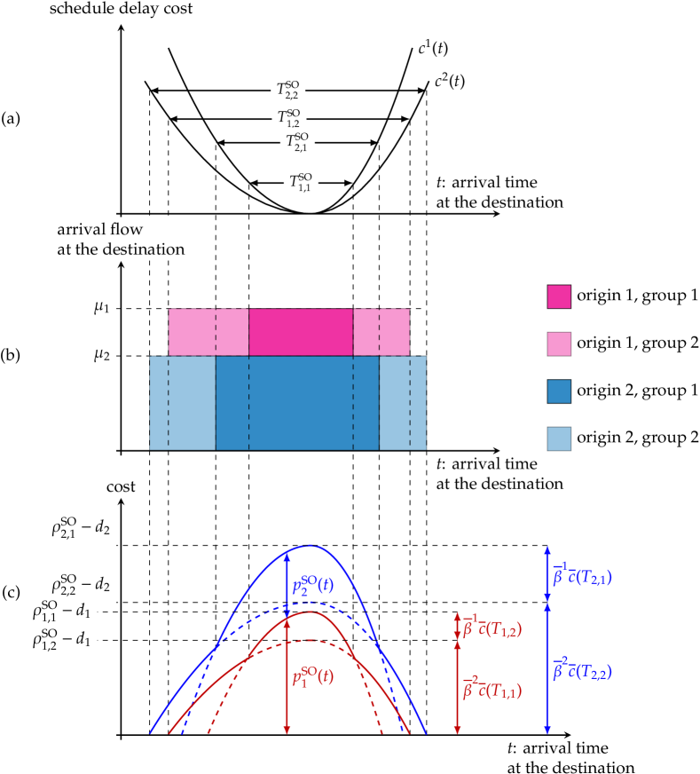
Figure 6: DSO solution.

4 Queue replacement principle and the dynamic user equilibrium problem

In this section, we prove the QRP and present an approach to construct a DUE solution using the DSO solution obtained in Section 3. Section 4.1 formulates the DUE problem according to Akamatsu et al. (2015). In Section 4.2, we prove the QRP and derive the analytical DUE solution. Finally, Section 4.3 compares the solutions and demonstrates the essential similarities and differences between the DSO and DUE states.

4.1 Formulation of the DUE problem

To formulate the DUE problem, we first introduce the commuter’s trip cost. As mentioned above, the commuter’s trip cost is measured based on the arrival time at the destination. It is assumed to be additively separable into schedule delay costs, queuing delay costs, and free-flow travel times. The trip cost of $(i,k)$-commuters arriving at time $t$ at the destination is defined as follows:

$$C_{i,k}(t)=\beta^{k}c(t)+\alpha\left(\sum_{j;j\leq i}w_{j}(t)+d_{i}\right) \forall i\in\mathcal{N},\quad\forall k\in\mathcal{K},\quad\forall t\in\mathcal{T},$$ (37)

where $\alpha$ is a parameter representing the value of time. This study assumes $\alpha=1$ regardless of the commuter’s group. In the DUE state, all commuters can not reduce their commuting costs by unilaterally changing their arrival time. This is expressed as the following linear complementarity condition:

$$\begin{dcases}\sum_{j;j\leq i}w^{\mathrm{UE}}_{j}(t)+\beta^{k}c(t)+d_{i}=\rho^{\mathrm{UE}}_{i,k}\quad&\mathrm{if}\quad q^{\mathrm{UE}}_{i,k}(t)>0\\ \sum_{j;j\leq i}w^{\mathrm{UE}}_{j}(t)+\beta^{k}c(t)+d_{i}\geq\rho^{\mathrm{UE}}_{i,k}\quad&\mathrm{if}\quad q^{\mathrm{UE}}_{i,k}(t)=0\end{dcases} \forall k\in\mathcal{K},\quad\forall i\in\mathcal{N},\quad\forall t\in\mathcal{T},$$ (38)

where $w^{\mathrm{UE}}_{i}(t)$ is a queueing delay cost for commuters arriving at time $t$ at the destination, and $\rho^{\mathrm{UE}}_{i,k}$ is an equilibrium commuting cost of the $(i,k)$-commuters. The superscript $\mathrm{UE}$ indicates that the variables are defined in the DUE problem.

In addition to the departure time choice condition (38), the queueing condition (11), demand conservation condition (5), and consistency condition (4) in Section 2 must be satisfied. Thus, the DUE problem is formulated as the following LCP:

[DUE-LCP]

Find $$\{\bm{q}^{\mathrm{UE}}(t)\}_{t\in\mathcal{T}},\{\bm{w}^{\mathrm{UE}}(t)\}_{t\in\mathcal{T}},\bm{\rho}^{\mathrm{UE}}$$

such that $$0\leq q^{\mathrm{UE}}_{i,k}(t)\perp\left\{\sum_{j;j\leq i}w^{\mathrm{UE}}_{j}(t)+\beta^{k}c(t)+d_{i}-\rho^{\mathrm{UE}}_{i,k}\right\}\geq 0 \forall k\in\mathcal{K},\quad\forall i\in\mathcal{N},\quad\forall t\in\mathcal{T},$$ (39)

$$0\leq w^{\mathrm{UE}}_{i}(t)\perp\left\{\mu_{i}\dot{\sigma}^{\mathrm{UE}}_{i}(t)-\sum_{j;j\geq i}q^{\mathrm{UE}}_{j}(t)\right\}\geq 0 \forall i\in\mathcal{N},\quad\forall t\in\mathcal{T},$$ (40)

$$0\leq\rho^{\mathrm{UE}}_{i,k}\perp\left\{\int_{\mathcal{T}}q^{\mathrm{UE}}_{i,k}(t)\mathrm{d}t-Q_{i,k}\right\}\geq 0 \forall k\in\mathcal{K},\quad\forall i\in\mathcal{N},$$ (41)

$$1-\sum_{j;j\leq i}\dot{w}^{\mathrm{UE}}_{j}(t)>0 \forall i\in\mathcal{N},\quad\forall t\in\mathcal{T}.$$ (42)

4.2 Queue replacement principle and the DUE solution

We first formally introduce the QRP concept in the multiple-bottleneck networks:

Definition 4.1 (QRP).

If there exists a DUE state such that the queueing delay pattern coincides with the optimal pricing pattern:

$$w^{\mathrm{UE}}_{i}(t)=p^{\mathrm{SO}}_{i}(t) \forall i\in\mathcal{N},\quad\forall t\in\mathcal{T},$$ (43)

then, the QRP holds.

We explore whether the QRP holds by deriving the equilibrium commuting cost and flow pattern that satisfy the DUE condition when $\{\bm{p}^{\mathrm{SO}}(t)\}_{t\in\mathcal{T}}$ is substituted for $\{\bm{w}^{\mathrm{UE}}(t)\}_{t\in\mathcal{T}}$. Consequently, we found that such an equilibrium cost and flow pattern exist if the schedule delay cost function satisfies certain conditions. We derive this conclusion from the following approach: First, by comparing the DSO problem’s optimality condition (15) and the DUE problem’s departure time choice condition (39), we observe that $\rho^{\mathrm{UE}}_{i,k}=\rho^{\mathrm{SO}}_{i,k}$ for all $(i,k)$-commuters. Second, based on this, we conjecture that arrival time window $\mathcal{T}^{\mathrm{UE}}_{i,k}\equiv\{t\in\mathcal{T}\mid q^{\mathrm{UE}}_{i,k}(t)>0\}$ is the same as the arrival time window in the DSO state $\mathcal{T}^{\mathrm{SO}}_{i,k}$ for all $(i,k)$-commuters. From this conjecture and the queueing delay condition (40), we can derive the flow pattern $\{\bm{q}(t)\}_{t\in\mathcal{T}}$ as follows:

$$q_{i,k}(t) =\begin{dcases}\mu_{i}\dot{\sigma}^{\mathrm{UE}}_{i}(t)-\mu_{(i+1)}\dot{\sigma}^{\mathrm{UE}}_{(i+1)}(t)&\mathrm{if}\quad t\in\mathcal{T}^{\mathrm{UE}}_{i,k}\setminus\mathcal{T}^{\mathrm{UE}}_{i,(k-1)}\\ 0&\mathrm{otherwise}\end{dcases} \forall k\in\mathcal{K},\quad\forall i\in\mathcal{N}.$$ (44)

However, this flow pattern can be negative, i.e., inconsistent with the departure time choice condition (39) of the DUE condition. Therefore, to prevent the negative flow, we introduce a condition of the schedule delay cost function described below. Finally, under this condition, we prove the conjecture by confirming that this flow pattern satisfies the demand conservation conditions.

Because this approach implies that there exist an equilibrium commuting cost and flow pattern that satisfy the DUE condition when $\{\bm{w}^{\mathrm{UE}}(t)\}_{t\in\mathcal{T}}=\{\bm{p}^{\mathrm{SO}}(t)\}_{t\in\mathcal{T}}$, we conclude that the QRP holds under the condition of the schedule delay cost function. This is summarized in the following theorem and proposition:

Theorem 4.1 (Sufficient condition for the QRP).

Suppose that the schedule delay cost function satisfies the following conditions:

$$\max\left\{-1,\quad-\dfrac{\mu_{i}-\mu_{(i+1)}}{\mu_{i}\beta^{\max}-\mu_{(i+1)}\beta^{\min}}\right\}<\dot{c}(t)<\dfrac{\mu_{i}-\mu_{(i+1)}}{\beta^{\max}\mu_{(i+1)}} \forall i\in\mathcal{N}\setminus\{N\},\quad\forall t\in\mathcal{T},$$ (45)

$$\text{where}\quad\beta^{\min}\equiv\min_{k\in\mathcal{K}}\left\{\beta^{k}\right\},\quad\beta^{\max}\equiv\max_{k\in\mathcal{K}}\left\{\beta^{k}\right\}.$$

Then, the QRP holds. We refer to the condition (45) as the QRP condition.

Proposition 4.1 (Solution to the DUE Problem).

Suppose that the QRP condition (45) holds. Then, the following $\{\bm{q}^{\mathrm{UE}}(t)\}_{t\in\mathcal{T}}$, $\{\bm{w}^{\mathrm{UE}}(t)\}_{t\in\mathcal{T}}$ and $\bm{\rho}^{\mathrm{UE}}$ are the solutions to [DUE-LCP]:

$$\mathcal{T}^{\mathrm{UE}}_{i,k} =\mathcal{T}^{\mathrm{SO}}_{i,k} \forall k\in\mathcal{K},\quad\forall i\in\mathcal{N}.$$ (46)

$$q^{\mathrm{UE}}_{i,k}(t) =\begin{dcases}\mu_{i}\dot{\sigma}^{\mathrm{UE}}_{i}(t)-\mu_{(i+1)}\dot{\sigma}^{\mathrm{UE}}_{(i+1)}(t)&\mathrm{if}\quad t\in\mathcal{T}^{\mathrm{UE}}_{i,k}\setminus\mathcal{T}^{\mathrm{UE}}_{i,(k-1)}\\ 0&\mathrm{otherwise}\end{dcases} \forall k\in\mathcal{K},\quad\forall i\in\mathcal{N},$$ (47)

$$w^{\mathrm{UE}}_{i}(t) =p^{\mathrm{SO}}_{i}(t) \forall i\in\mathcal{N},\quad\forall t\in\mathcal{T},$$ (48)

$$\rho^{\mathrm{UE}}_{i,k} =\rho^{\mathrm{SO}}_{i,k} \forall k\in\mathcal{K},\quad\forall i\in\mathcal{N},$$ (49)

where $$\quad\sigma^{\mathrm{UE}}_{i}(t)=t-\sum_{j;j\leq i}w^{\mathrm{UE}}_{j}(t) \forall i\in\mathcal{N},\quad\forall t\in\mathcal{T}.$$ (50)

Considering $\beta^{k}\in(0,1]$ for all $k\in\mathcal{K}$, we can simplify the QRP condition (45) to make it independent of $\{\beta^{k}\}$ as follows:

$$\dfrac{\mu_{(i+1)}}{\mu_{i}}-1<\dot{c}(t)<\dfrac{\mu_{i}}{\mu_{(i+1)}}-1 \forall i\in\mathcal{N}\setminus\{N\},\quad\forall t\in\mathcal{T}.$$ (51)

This condition (51) is a sufficient condition for the condition (45). Note that the condition (51) always holds $\dot{c}(t)>-1$ because $\mu_{i+1}/\mu_{i}>0$.

4.3 Comparison between the DUE and DSO solutions

We now compare the flow patterns of the DSO and DUE states, and discuss their relationships. Figure 7 illustrates the arrival flow pattern at the destination in the DSO state (upper figure) and DUE state (lower figure). Both arrival flow patterns are similar in terms of arrival time windows of commuters and the only difference is the destination arrival flow rates at every moment. Specifically, the arrival time windows of $(i,k)$-commuters in the DSO and DUE states are equal. Therefore, the sorting properties hold for both the DSO and DUE states. However, the destination arrival flow rates of the DUE state differ from those of the DSO state because of the congestion effect of $\dot{\sigma}^{\mathrm{UE}}_{i}(t)$. According to the definition of $\sigma_{i}(t)$, the congestion effect $\dot{\sigma}^{\mathrm{UE}}_{i}(t)$ is determined by the queueing delay pattern, and we find that the queueing delay pattern depends on the schedule delay cost function according to Eqs. 34 and 47.

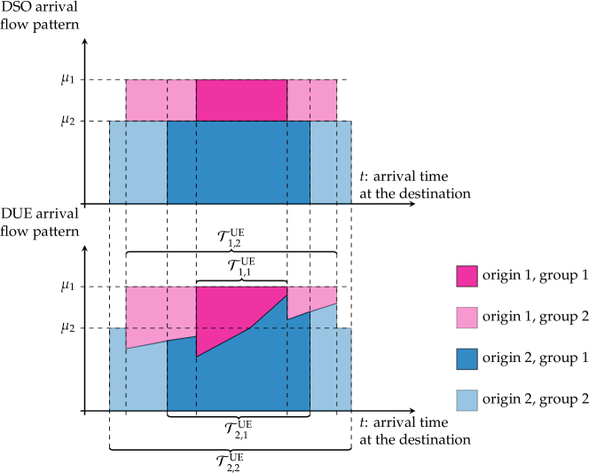
Figure 7: DSO and DUE arrival flow pattern at the destination.

We discuss the pricing patterns in the DSO state and queueing patterns in the DUE state. We find that Pareto improvement can be achieved if the road manager imposes dynamic pricing that mimics the queueing delay pattern in the DUE state. Two significant properties of Proposition 4.1 confirm this fact: 1) the DSO pricing patterns are the same as the DUE queuing delay patterns at each bottleneck; and 2) the DSO trip cost of each commuter (schedule delay costs + congestion prices) is equal to the DUE trip cost (schedule delay costs + queuing delay costs).

Based on these properties, we find that the road manager’s cost can be decreased by imposing the pricing equal to the queuing delay because the road manager gains revenue equal to the total queuing delay cost. In other words, the road manager’s benefit improves without increasing anyone’s equilibrium commuting cost, thereby achieving the Pareto improvement. This is summarized in the following theorem.

Theorem 4.2 (Pareto improvement).

Suppose that the QRP condition (45) holds. If the road manager imposes the dynamic pricing equal to the queuing delay $\{w^{\mathrm{UE}}_{i}(t)\}_{t\in\mathcal{T}}$ at all bottlenecks $i\in\mathcal{N}$, the road manager’s benefit improves without increasing anyone’s equilibrium commuting cost

These results do not contradict those of previous studies that proposed that the optimal pricing does not achieve Pareto improvement when heterogeneous commuters exist (e.g., Arnott et al. (1988, 1994); van den Berg and Verhoef (2010, 2011); Hall (2021)). This is because these studies assume commuters’ heterogeneity in terms of the value of time (i.e., parameter $\alpha$ in Eq. 37 differs for each group, unlike the model of this study. Theorem 4.2 proposes that such inequity does not occur when the commuters’ heterogeneity is considered in terms of the value of schedule delay.

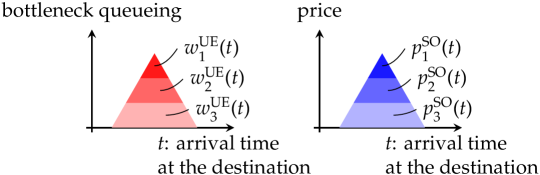
Figure 8: Simplified graphical images of bottleneck queueing and pricing patterns in a three-link network.

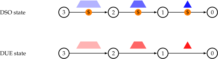
Figure 9: Example of the QRP in a three-link network.

4.4 Application of the QRP to the partial bottleneck pricing

Thus far, we have discussed that the QRP enables us to derive the DUE state by replacing the optimal pricing pattern with a bottleneck queueing delay pattern. In this section, we focus on the case when pricing is introduced only for some bottlenecks and consider the equilibrium under the partial bottleneck pricing.

We consider the case in which the optimal pricing is introduced to some bottlenecks $\mathcal{N}^{\mathrm{P}}\subseteq\mathcal{N}$ (hereafter referred to as partial bottleneck pricing: PBP). In this case, the trip cost of $(i,k)$-commuters arriving at the destination at time $t$ is calculated as follows:

$$C^{\mathrm{PBP}}_{i,k}(t)=\sum_{j;j\leq i}w^{\mathrm{PBP}}_{j}(t)+\left(\beta^{k}c(t)+\sum_{j;j\in\mathcal{N}^{\mathrm{P}},j\leq i}p^{\mathrm{SO}}_{j}(t)\right)+d_{i} \forall k\in\mathcal{K},\quad\forall i\in\mathcal{N},\quad\forall t\in\mathcal{T},$$ (52)

where $w^{\mathrm{PBP}}_{i}(t)$ represents the queueing delay at bottleneck $i$ for the commuters arriving at time $t$ at the destination. The equilibrium state under the PBP can be obtained as the solution to the following LCP:

[DUE-PBP]

Find $$\{\bm{q}^{\mathrm{PBP}}(t)\}_{t\in\mathcal{T}},\{\bm{w}^{\mathrm{PBP}}(t)\}_{t\in\mathcal{T}},\bm{\rho}^{\mathrm{PBP}},$$

such that $$0\leq q^{\mathrm{PBP}}_{i,k}(t)\perp\left\{C^{\mathrm{PBP}}_{i,k}(t)-\rho^{\mathrm{PBP}}_{i,k}\right\}\geq 0 \forall k\in\mathcal{K},\quad\forall i\in\mathcal{N},\quad\forall t\in\mathcal{T},$$ (53)

$$0\leq w^{\mathrm{PBP}}_{i}(t)\perp\left\{\mu_{i}\dot{\sigma}^{\mathrm{PBP}}_{i}(t)-\sum_{j;j\geq i}q^{\mathrm{PBP}}_{j}(t)\right\}\geq 0 \forall i\in\mathcal{N}\setminus\mathcal{N}^{\mathrm{P}},\quad\forall t\in\mathcal{T},$$ (54)

$$0\leq\rho^{\mathrm{PBP}}_{i,k}\perp\left\{\int_{\mathcal{T}}q^{\mathrm{PBP}}_{i,k}(t)\mathrm{d}t-Q_{i,k}\right\}\geq 0 \forall k\in\mathcal{K},\quad\forall i\in\mathcal{N},$$ (55)

$$\dot{\tau}^{\mathrm{PBP}}_{i}(t)>0 \forall i\in\mathcal{N},\quad\forall t\in\mathcal{T}.$$ (56)

The first condition (53) represents the departure time choice condition. The second condition (54) represents the dynamics of the queueing at bottleneck $i\in\mathcal{N}\setminus\mathcal{N}^{\mathrm{P}}$. The third condition (55) represents the demand conservation condition. The final condition (56) represents the consistency condition.

Interestingly, if the pricing bottleneck set $\mathcal{N}^{\mathrm{P}}$ satisfies a certain condition, the queueing delay pattern at no-pricing bottleneck under the PBP equals that in the DUE state, i.e., $w^{\mathrm{PBP}}_{i}(t)=w^{\mathrm{UE}}_{i}(t)$, $\forall i\in\mathcal{N}\setminus\mathcal{N}^{\mathrm{P}}$. Moreover, using this queueing delay pattern, we can construct the equilibrium flow pattern under the PBP, just like deriving the DUE solution. To derive the solution in this way, we introduce the following assumption:

Assumption 4.1.

The pricing bottlenecks are located contiguously from the most upstream bottleneck $N$. That is, the pricing bottleneck set $\mathcal{N}^{\mathrm{P}}\subseteq\mathcal{N}$ can always be written as follows:

$$\mathcal{N}^{\mathrm{P}}=\left\{i^{\mathrm{PBP}},i^{\mathrm{PBP}}+1,...,N\right\},$$ (57)

where $i^{\mathrm{PBP}}\in\mathcal{N}$ is the most downstream pricing bottleneck.

In situations where this assumption holds, the queueing pattern under the PBP satisfies the consistency condition (56), which is the condition to guarantee a physically feasible flow in the Lagrangian coordinate approach as mentioned in Section 2. Indeed, $\dot{\tau}^{\mathrm{PBP}}_{i}(t)$ is calculated as follows:

$$\dot{\tau}^{\mathrm{PBP}}_{i}(t) =1-\sum_{j;j\leq i}\dot{w}^{\mathrm{PBP}}_{j}=\begin{dcases}\dot{\tau}^{\mathrm{UE}}_{i}(t)\quad&\mathrm{if}\quad i\in\mathcal{N}\setminus\mathcal{N}^{\mathrm{P}}\\ \dot{\tau}^{\mathrm{UE}}_{(i^{\mathrm{PBP}}-1)}(t)\quad&\mathrm{if}\quad i\in\mathcal{N}^{\mathrm{P}}\end{dcases} \forall i\in\mathcal{N}\setminus\{1\},\quad\forall t\in\mathcal{T},$$ (58)

because the PBP eliminates the queue at the pricing bottleneck $i\in\mathcal{N}^{\mathrm{P}}$ and maintains the queue at the unpriced bottleneck $i\in\mathcal{N}\setminus\mathcal{N}^{\mathrm{P}}$. Because $\dot{\tau}^{\mathrm{UE}}_{i}(t)>0$, $\forall i\in\mathcal{N}$, $\forall t\in\mathcal{T}$, we can confirm that the consistency condition (56) holds under Assumption 4.1. Thus, this assumption is the sufficient condition for the queueing delay pattern $w^{\mathrm{UE}}_{i}(t)$, $\forall i\in\mathcal{N}\setminus\mathcal{N}^{\mathrm{P}}$ not to contradict the equilibrium condition under the PBP.

If we accept Assumption 4.1, we obtain the solutions to [DUE-PBP] using the QRP:

Lemma 4.1.

Suppose that the QRP condition (45) and Assumption 4.1 hold. Then, the following $\{\bm{q}^{\mathrm{PBP}}(t)\}_{t\in\mathcal{T}}$, $\{\bm{w}^{\mathrm{PBP}}(t)\}_{t\in\mathcal{T}}$ and $\bm{\rho}^{\mathrm{PBP}}$ are the solutions to [DUE-PBP]:

$$q^{\mathrm{PBP}}_{i,k}(t)=\begin{dcases}\mu_{i}\dot{\sigma}^{\mathrm{PBP}}_{i}(t)-\mu_{(i+1)}\dot{\sigma}^{\mathrm{PBP}}_{(i+1)}(t)\quad&\mathrm{if}\quad t\in\mathcal{T}^{\mathrm{UE}}_{i,k}\setminus\mathcal{T}^{\mathrm{UE}}_{i,(k-1)}\\ 0&\mathrm{otherwise}\end{dcases} \forall i\in\mathcal{N},$$ (59)

$$\rho^{\mathrm{PBP}}_{i,k}=\rho^{\mathrm{UE}}_{i,k} \forall i\in\mathcal{N},$$ (60)

$$w^{\mathrm{PBP}}_{i}(t)=\begin{dcases}w^{\mathrm{UE}}_{i}(t)\quad&\mathrm{if}\quad i\in\mathcal{N}\setminus\mathcal{N}^{\mathrm{P}}\\ 0\quad&\mathrm{if}\quad i\in\mathcal{N}^{\mathrm{P}}\end{dcases} \forall t\in\mathcal{T}.$$ (61)

Lemma 4.1 can be proven using a similar approach to the proof of footnote 6. Specifically, when queues at the bottleneck with pricing are replaced by zero, and the queues at the bottleneck without pricing are replaced by $p$, we show that these queueing delay patterns satisfy the DUE condition under the PBP.

Let us consider the queueing delay patterns that occur under the PBP. For convenience, we introduce Figures 8 and 9, which illustrate a simple example of the QRP in a three-link network. Figure 8 depicts the pricing and queueing patterns in a three-link network. The approximate shapes of both patterns are represented by triangles and trapezoids. Using these graphic representations, Figure 9 shows the QRP in which the DSO pricing patterns are the same as the DUE queuing delay patterns at each bottleneck. Figure 10 depicts an equilibrium state under the pricing at Bottleneck $3$, i.e., $\mathcal{N}^{\mathrm{P}}=\{3\}$. Because the road manager imposes tolling $p^{\mathrm{SO}}_{3}(t)$ at Bottleneck $3$, the queueing at Bottleneck $3$ is completely eliminated. Conversely, the bottleneck queueing is formed at Bottlenecks $1$ and $2$, thus, maintaining the same equilibrium commuting cost. Consequently, the bottleneck queueing at Bottlenecks $1$ and $2$ is shown in Figure 10. As shown in Lemma 4.1, this equilibrium state has two essential features: (i) the queueing delay pattern at bottleneck $i\in\mathcal{N}\setminus\mathcal{N}^{\mathrm{P}}$ is equal to that in the DUE state, and (ii) the equilibrium commuting cost of each commuter is equal to that in the DUE (DSO) state.

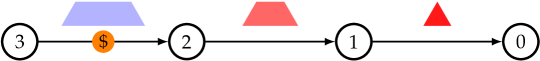
Figure 10: Equilibrium under the partial bottleneck pricing (PBP).

By comparing the solutions to the [DSO], [DUE], and [DUE-PBP], we obtain the following theorem:

Theorem 4.3.

Suppose that the QRP condition (45) and Assumption 4.1 hold.

(a) The equilibrium commuting cost of $(i,k)$-commuters under the PBP is equal to that in the DSO and DUE states:

$$\rho^{\mathrm{PBP}}_{i,k}=\rho^{\mathrm{SO}}_{i,k}=\rho^{\mathrm{UE}}_{i,k} \forall k\in\mathcal{K},\quad\forall i\in\mathcal{N}.$$ (62)

(b) The total system costs satisfy the following inequality:

$$Z^{\mathrm{SO}}\leq Z^{\mathrm{PBP}}(\mathcal{N}^{\mathrm{P}})\leq Z^{\mathrm{UE}},$$ (63)

where $Z^{\mathrm{SO}}$ and $Z^{\mathrm{UE}}$ are the total system costs of the DSO and DUE states, respectively. The equality in the LHS of Eq. 63 holds if and only if $\mathcal{N}^{\mathrm{P}}=\mathcal{N}$ and the equality in the RHS of Eq. 63 holds if and only if $\mathcal{N}^{\mathrm{P}}=\emptyset$.

Theorem 4.3 implies that we can improve the system cost by partially implementing dynamic pricing on bottlenecks without considering the influence of such an implementation on the other bottlenecks. In addition, the road manager gains revenue equal to the sum of queuing delay costs at the bottlenecks with pricing. In other words, the partial bottleneck pricing can achieve the Pareto improvement under Assumption 4.1 and the QRP condition. Therefore, because of Theorems 4.2 and 4.3, we can interpret the QRP condition as a sufficient condition for a Pareto improvement by full/partial optimal pricing. A similar result was shown by Fu et al. (2022), assuming homogeneous commuters; however, the remarkable difference is that the pricing bottleneck set condition (Assumption 4.1) is required.

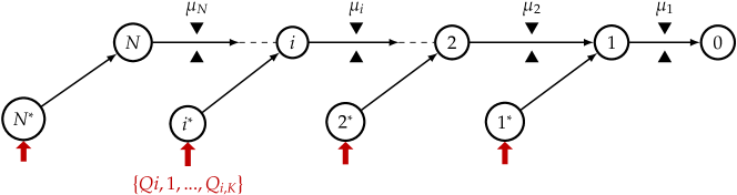
Figure 11: Corridor network with on-ramp links.

5 Applications of the QRP to on-ramp-based policies

The QRP and PBP analyses results represent a replaceability of commuters’ costs in the departure time choice problem under several conditions. This replaceability means that as long as each commuter’s commuting cost is equal to those in the DUE and DSO states, a feasible flow pattern exists regardless of whether the costs experienced at the links are queuing or price costs. Such link cost replaceability leads us to expect the same kind of replaceability for the node-based (on-ramp-based) cost. For example, the queueing at the on-ramp under the on-ramp metering may coincide with the pricing pattern under the on-ramp pricing. If such replaceability (equivalence) also holds, we can construct a systematic approach for analyzing the on-ramp-based and bottleneck-based policies based on the QRP.

This section considers the two on-ramp-based policies: on-ramp metering and on-ramp pricing to gain an insight into the theoretical relationship between the on-ramp-based and bottleneck-based policies. We demonstrate that the QRP enables us to obtain equilibrium solutions under the on-ramp-based policies. Section 5.1 analyzes the case in which metering/pricing is implemented at all on-ramps (hereafter referred to as full implementation) and derives the equilibrium solution using the QRP. Section 5.2 analyzes the case when metering/pricing is only implemented at partial on-ramps (hereafter referred to as partial implementation) and derives the equilibrium solution to this case. Section 5.3 discusses the theoretical properties of these policies by comparing these equilibrium solutions in the DSO and DUE solutions. In the remainder of this section, we assume that the QRP schedule delay cost function satisfies Eq. 45.

We consider the extended network with on-ramp links and nodes. As shown in Figure 11, we add on-ramp link $i^{\ast}$ representing the access link that connects nodes $i$ and $i^{\ast}$. Free-flow travel times of on-ramp links are assumed to be zero, and the set of on-ramp links is defined by $\mathcal{N}^{\ast}$. The arrival flow variables are defined by $q_{i^{\ast}}(t)$ using $i^{\ast}$ instead of $q_{i}(t)$. We define $w_{i^{\ast}}(t)$ as the queueing delay at on-ramp $i^{\ast}$ created by the on-ramp metering for the commuters whose destination arrival time is $t$.

5.1 Full implementation policies

5.1.1 Full on-ramp metering

On-ramp metering (RM) is one of the most common methods used for managing freeway traffic. The primary strategy of ramp metering is to maintain the freeway traffic by adjusting the inflow rate from the on-ramp. This study considers ramp metering, which aims to eliminate queues on the freeway. For all on-ramps $i^{\ast}\in\mathcal{N}^{\ast}$, we set the metering rate to $\mu_{i^{\ast}}=\overline{\mu}_{i}$ because $\overline{\mu}_{i}$ is the maximum value without creating a queue at the downstream bottleneck $i$ on the freeway.

We consider the equilibrium under the on-ramp metering for all ramps (full on-ramp metering). The associated equilibrium problem is the following LCP:

[DUE-RM]

Find $$\{\bm{q}(t)\}_{t\in\mathcal{T}},\{\bm{w}(t)\}_{t\in\mathcal{T}},\bm{\rho}$$

such that $$0\leq q_{i^{\ast},k}(t)\perp\left\{w_{i^{\ast}}(t)+\beta^{k}c(t)+d_{i}-\rho_{i^{\ast},k}\right\}\geq 0 \forall k\in\mathcal{K},\quad\forall i\in\mathcal{N},\quad\forall t\in\mathcal{T},$$ (64)

$$0\leq w_{i^{\ast}}(t)\perp\left\{\overline{\mu}_{i}-q_{i^{\ast}}(t)\right\}\geq 0 \forall i^{\ast}\in\mathcal{N}^{\ast},\quad\forall t\in\mathcal{T},$$ (65)

$$0\leq\rho_{i^{\ast},k}\perp\left\{\int_{\mathcal{T}}q_{i^{\ast},k}(t)\mathrm{d}t-Q_{i,k}\right\}\geq 0 \forall k\in\mathcal{K},\quad\forall i^{\ast}\in\mathcal{N}^{\ast},$$ (66)

$$\dot{\tau}_{i^{\ast}}(t)>1 \forall i^{\ast}\in\mathcal{N}^{\ast}.$$ (67)

Condition (65) represents the queueing dynamics at each on-ramp $i^{\ast}\in\mathcal{N}^{\ast}$.

The problem [DUE-RM] has a similar mathematical structure to the problem [DUE], particularly, for the departure time choice condition of [DUE-RM] and [DUE] (Eqs. 64 and 39), if $w_{i^{\ast}}(t)$ is regarded as $\sum_{j;j\leq i}w^{\mathrm{UE}}_{j}(t)$, then the form is exactly the same. This fact leads us to expect each commuter’s commuting costs of [DUE-RM] to be equal to those of [DUE]. This expectation is actually true. We confirm this by constructing the solution to [DUE-RM] using the equilibrium condition of [DUE-RM] and the solution to [DUE]. The solution to [DUE-RM] is shown as follows:

Lemma 5.1.

The following $\{\bm{q}^{\mathrm{RM}}(t)\}_{t\in\mathcal{T}}$, $\{\bm{w}^{\mathrm{RM}}(t)\}_{t\in\mathcal{T}}$, and $\bm{\rho}^{\mathrm{RM}}$ are equilibrium solutions to [DUE-RM]:

$$q^{\mathrm{RM}}_{i^{\ast},k}(t)=\begin{dcases}\overline{\mu}_{i}&\mathrm{if}\quad t\in\mathcal{T}^{\mathrm{UE}}_{i,k}\setminus\mathcal{T}^{\mathrm{UE}}_{i,(k-1)}\\ 0&\mathrm{otherwise}\end{dcases} \forall k\in\mathcal{K},\quad\forall i\in\mathcal{N},\quad\forall t\in\mathcal{T}.$$ (68)

$$w^{\mathrm{RM}}_{i^{\ast}}(t)=\sum_{j;j\leq i}w^{\mathrm{UE}}_{j}(t) \forall i^{\ast}\in\mathcal{N}^{\ast},\quad\forall t\in\mathcal{T},$$ (69)

$$\rho^{\mathrm{RM}}_{i,k}=\rho^{\mathrm{UE}}_{i,k} \forall k\in\mathcal{K},\quad\forall i\in\mathcal{N}.$$ (70)

Figure 12 depicts the solution to [DUE-RM] in the case of a three-link network. We find that the queueing delay at each on-ramp $w^{\mathrm{RM}}_{i^{\ast}}(t)$ is equal to the sum of queueing delays at its downstream bottlenecks in the DUE state $\sum_{j;j\leq i}w^{\mathrm{UE}}_{j}(t)$.

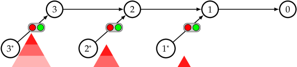
Figure 12: Equilibrium under the on-ramp metering (RM).

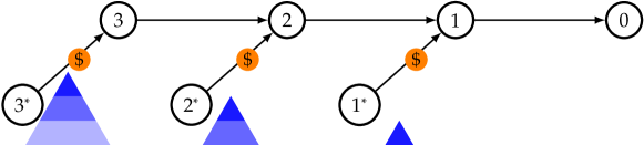
Figure 13: Equilibrium under the on-ramp pricing (RP).

5.1.2 Full on-ramp pricing

We consider the equilibrium under the on-ramp pricing. In this case, the road manager imposes the toll at all on-ramps. We assume that the road manager tolled $p^{\mathrm{RP}}_{i^{\ast}}(t)=\sum_{j;j\leq i}p^{\mathrm{SO}}_{j}(t)$ at on-ramp $i^{\ast}$. The associated equilibrium problem is the following LCP:

[DUE-RP]

Find $$\{\bm{q}(t)\}_{t\in\mathcal{T}},\{\bm{w}(t)\}_{t\in\mathcal{T}},\bm{\rho}$$

such that $$0\leq q_{i^{\ast},k}(t)\perp\left\{p^{\mathrm{RP}}_{i^{\ast}}(t)+w_{i^{\ast}}(t)+\beta^{k}c(t)+d_{i}-\rho_{i^{\ast},k}\right\}\geq 0 \forall k\in\mathcal{K},\quad\forall i\in\mathcal{N},\quad\forall t\in\mathcal{T},$$ (71)

$$0\leq w_{i^{\ast}}(t)\perp\left\{\overline{\mu}_{i}-q^{\mathrm{RP}}_{i^{\ast}}(t)\right\}\geq 0 \forall i^{\ast}\in\mathcal{N}^{\ast},\quad\forall t\in\mathcal{T},$$ (72)

$$0\leq\rho_{i^{\ast},k}\perp\left\{\int_{\mathcal{T}}q_{i^{\ast},k}(t)\mathrm{d}t-Q_{i,k}\right\}\geq 0 \forall k\in\mathcal{K},\quad\forall i^{\ast}\in\mathcal{N}^{\ast},$$ (73)

$$\dot{\tau}_{i^{\ast}}(t)>1 \forall i^{\ast}\in\mathcal{N}^{\ast}.$$ (74)

Condition (72) represents the queueing dynamics at each bottleneck $i\in\mathcal{N}$. The queues at all ramps are completely eliminated by the on-ramp pricing ($w^{\mathrm{RP}}_{i^{\ast}}(t)=0$, $\forall i^{\ast}\in\mathcal{N}^{\ast}$, $\forall t\in\mathcal{T}$).

Using an approach similar to that of [DUE-RM], we obtain the solution to [DUE-RP] as follows:

Lemma 5.2.

The following $\{\bm{q}^{\mathrm{RP}}(t)\}_{t\in\mathcal{T}}$, $\{\bm{w}^{\mathrm{RP}}(t)\}_{t\in\mathcal{T}}$, and $\bm{\rho}^{\mathrm{RP}}$ are equilibrium solutions to [DUE-RP]:

$$q^{\mathrm{RP}}_{i^{\ast},k}(t)=\begin{dcases}\overline{\mu}_{i}&\mathrm{if}\quad t\in\mathcal{T}^{\mathrm{UE}}_{i,k}\setminus\mathcal{T}^{\mathrm{UE}}_{i,(k-1)}\\ 0&\mathrm{otherwise}\end{dcases} \forall k\in\mathcal{K},\quad\forall i\in\mathcal{N},\quad\forall t\in\mathcal{T}.$$ (75)

$$w^{\mathrm{RP}}_{i^{\ast}}(t)=0 \forall i^{\ast}\in\mathcal{N}^{\ast},\quad\forall t\in\mathcal{T},$$ (76)

$$\rho^{\mathrm{RP}}_{i,k}=\rho^{\mathrm{UE}}_{i,k} \forall k\in\mathcal{K},\quad\forall i\in\mathcal{N},$$ (77)

Figure 13 depicts the equilibrium state under the on-ramp pricing. We see that the queueing is equal to the on-ramp pricing at each on-ramp.

5.2 Partial implementation policies

5.2.1 Partial on-ramp metering

We consider the partial on-ramp metering and define the set of links with the on-ramp meter as $\mathcal{N}^{\ast\mathrm{P}}\subseteq\mathcal{N}^{\ast}$. The associated equilibrium problem is the following LCP:

[DUE-PRM]

Find $$\{\bm{q}(t)\}_{t\in\mathcal{T}}\{w_{i}(t)\}_{i\in\mathcal{N},t\in\mathcal{T}},\{w_{i^{\ast}}(t)\}_{i^{\ast}\in\mathcal{N}^{\ast},t\in\mathcal{T}},\bm{\rho},$$

such that $$0\leq q_{i^{\ast},k}(t)\perp\left\{w_{i^{\ast}}(t)+\sum_{j;j<i}w_{j}(t)+\beta^{k}c(t)+d_{i}-\rho_{i^{\ast},k}\right\}\geq 0 \forall i^{\ast}\in\mathcal{N}^{\ast},\forall k\in\mathcal{K},\quad\forall t\in\mathcal{T},$$ (78)

$$0\leq w_{i}(t)\perp\left\{\mu_{i}\dot{\sigma}_{i}(t)-\sum_{j^{\ast};j^{\ast}\geq i^{\ast}}q_{j^{\ast}}(t)\right\}\geq 0 \forall i\in\mathcal{N}\setminus\mathcal{N}^{\ast\mathrm{P}},\quad\forall t\in\mathcal{T},$$ (79)

$$0\leq w_{i^{\ast}}(t)\perp\left\{\overline{\mu}_{i}\dot{\sigma}_{i^{\ast}}(t)-q_{i^{\ast}}(t)\right\}\geq 0 \forall i^{\ast}\in\mathcal{N}^{\ast\mathrm{P}},\quad\forall t\in\mathcal{T},$$ (80)

$$0\leq\rho_{i,k}\perp\left\{\int_{\mathcal{T}}q_{i^{\ast},k}(t)\mathrm{d}t-Q_{i,k}\right\}\geq 0 \forall k\in\mathcal{K},\quad\forall i\in\mathcal{N},$$ (81)

$$\dot{\tau}_{j}(t)>0 \forall j\in\mathcal{N}\cup\mathcal{N}^{\ast},\quad\forall t\in\mathcal{T}.$$ (82)

The first condition (78) represents the departure time choice condition of each $(i^{\ast},k)$-commuters. Commuters who depart from origin $i^{\ast}\in\mathcal{N}^{\ast\mathrm{P}}$ are constrained by the on-ramp metering. Conditions (79) and (80) represent the queueing dynamics at each bottleneck $i\in\mathcal{N}\setminus\mathcal{N}^{\ast\mathrm{P}}$ and each on-ramp $i\in\mathcal{N}^{\ast\mathrm{P}}$, respectively.

Although the [DUE-PRM] appears to be a complex equilibrium problem at first glance, we obtain the solution by applying the methods discussed previously. The basic approach for obtaining the solution is the same as in the case of partial bottleneck pricing. Specifically, the approach is based on the conjecture that the equilibrium commuting cost of each commuter is equal to that in the DUE (DSO) state. Based on this conjecture, we derive the solution to [DUE-PRM] using the equilibrium condition of [DUE-PRM] and the DUE solution. We subsequently confirm that the conjecture is true. Consequently, we analytically obtain the solutions to [DUE-PRM]:

Lemma 5.3.

The following $\{\bm{q}^{\mathrm{PRM}}(t)\}_{t\in\mathcal{T}}$ $\{w^{\mathrm{PRM}}_{i}(t)\}_{i\in\mathcal{N},t\in\mathcal{T}}$, $\{w^{\mathrm{PRM}}_{i^{\ast}}(t)\}_{i^{\ast}\in\mathcal{N}^{\ast},t\in\mathcal{T}}$, and $\bm{\rho}^{\mathrm{PRM}}$ are the equilibrium solution to [DUE-PRM]:

$$\rho^{\mathrm{PRM}}_{i,k}=\rho^{\mathrm{UE}}_{i,k} \forall i\in\mathcal{N},$$ (83)

$$w^{\mathrm{PRM}}_{i}(t)=\begin{dcases}0\quad&\mathrm{if}\quad i\in\mathcal{N}^{\ast\mathrm{P}}\\ \sum_{j\in\mathcal{N}^{\ast\mathrm{P}};j\leq i}w^{\mathrm{UE}}_{j}(t)\quad&\mathrm{if}\quad i\in\mathcal{N}\setminus\mathcal{N}^{\ast\mathrm{P}}\end{dcases} \forall t\in\mathcal{T},$$ (84)

$$w^{\mathrm{PRM}}_{i\ast}(t)=\begin{dcases}\sum_{j\in\mathcal{N}^{\ast}\setminus\mathcal{N}^{\ast\mathrm{P}};j\leq i}w^{\mathrm{UE}}_{j}(t)\quad&\mathrm{if}\quad i\in\mathcal{N}^{\ast\mathrm{P}}\\ 0\quad&\mathrm{if}\quad i\in\mathcal{N}^{\ast}\setminus\mathcal{N}^{\ast\mathrm{P}}\end{dcases} \forall t\in\mathcal{T},$$ (85)

$$q^{\mathrm{PRM}}_{i^{\ast},k}(t)=\begin{dcases}\mu_{i}\dot{\sigma}^{\mathrm{PRM}}_{i}(t)-\mu_{(i+1)}\dot{\sigma}^{\mathrm{PRM}}_{(i+1)}(t)\quad&\mathrm{if}\quad t\in\mathcal{T}^{\mathrm{UE}}_{i,k}\\ 0\quad&\mathrm{if}\quad t\notin\mathcal{T}^{\mathrm{UE}}_{i,k}\end{dcases} \forall i\in\mathcal{N}.$$ (86)

Figure 14 depicts the equilibrium state under the on-ramp metering at Link $3$, i.e., $\mathcal{N}^{\ast\mathrm{P}}=\{3\}$. The on-ramp queueing delay pattern at Link $3$ is equal to the pattern under all on-ramp metering cases, and there is no queueing at Bottleneck $3$. Moreover, the bottleneck queues are formed at Bottlenecks $1$ and $2$, maintaining the same equilibrium commuting cost. The bottleneck queues at Bottlenecks $1$ and $2$ are shown in Figure 14. Any combination of ramps with metering is acceptable. For example, Figure 14 depicts the equilibrium state under the on-ramp metering at Link $2$, i.e., $\mathcal{N}^{\ast\mathrm{P}}=\{2\}$.

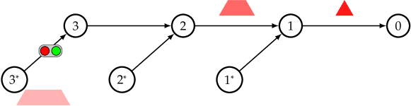
(a) Case of $\mathcal{N}^{\ast\mathrm{P}}=\{3\}$

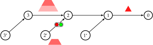
(b) Case of $\mathcal{N}^{\ast\mathrm{P}}=\{2\}$

Figure 14: Equilibrium under the partial on-ramp metering (PRM).

5.2.2 Partial on-ramp pricing

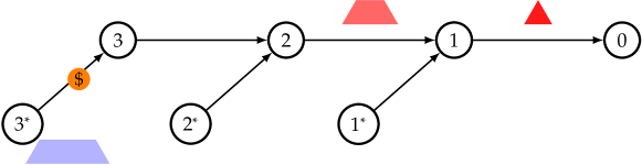
(a) Case of $\mathcal{N}^{\ast\mathrm{P}}=\{3\}$

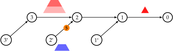
(b) Case of $\mathcal{N}^{\ast\mathrm{P}}=\{2\}$

Figure 15: Equilibrium under the partial on-ramp pricing (PRP).

We now consider the partial on-ramp pricing. Let $\mathcal{N}^{\ast\mathrm{P}}$ be a set of links with pricing. Assuming that the road manager tolled $p^{\mathrm{RP}}_{i^{\ast}}(t)$ at on-ramp $i^{\ast}\in\mathcal{N}^{\ast\mathrm{P}}$, the associated equilibrium problem is the following LCP:

[DUE-PRP]

Find $$\{\bm{q}(t)\}_{t\in\mathcal{T}}\{\bm{w}(t)\}_{t\in\mathcal{T}},\bm{\rho},$$

such that $$0\leq q_{i^{\ast},k}(t)\perp\left\{\sum_{j;j\leq i}w_{j}(t)+\beta^{k}c(t)+p^{\mathrm{RP}}_{i^{\ast}}(t)+d_{i}-\rho_{i,k}\right\}\geq 0 \forall k\in\mathcal{K},\quad\forall i^{\ast}\in\mathcal{N}^{\ast\mathrm{P}},\quad\forall t\in\mathcal{T},$$ (87)

$$0\leq w_{i}(t)\perp\left\{\mu_{i}\dot{\sigma}_{i}(t)-\sum_{j;j\geq i}q_{j}(t)\right\}\geq 0 \forall i\in\mathcal{N},\quad\forall t\in\mathcal{T},$$ (88)

$$0\leq\rho_{i,k}\perp\left\{\int_{\mathcal{T}}q_{i,k}(t)\mathrm{d}t-Q_{i,k}\right\}\geq 0 \forall k\in\mathcal{K},\quad\forall i\in\mathcal{N},$$ (89)

$$\dot{\tau}_{j}(t)>0 \forall j\in\mathcal{N}\cup\mathcal{N}^{\ast},\quad\forall t\in\mathcal{T}.$$ (90)

Condition (87) represents the departure time choice condition of each commuter.

We also obtain the equilibrium solution to [DUE-PRP] using an approach similar to that used in the case of [DUE-PRM]. Consequently, we obtain the following equilibrium solution:

Lemma 5.4.

The following $\{\bm{q}^{\mathrm{PRP}}(t)\}_{t\in\mathcal{T}}$ $\{\bm{w}^{\mathrm{PRP}}(t)\}_{t\in\mathcal{T}}$, and $\bm{\rho}^{\mathrm{PRP}}$ are the equilibrium solutions to [DUE-PRP]:

$$q^{\mathrm{PRP}}_{i^{\ast},k}(t)=\begin{dcases}\mu_{i}\dot{\sigma}^{\mathrm{PBP}}_{i}(t)-\mu_{(i+1)}\dot{\sigma}^{\mathrm{PBP}}_{(i+1)}(t)\quad&\mathrm{if}\quad t\in\mathcal{T}^{\mathrm{UE}}_{i,k}\setminus\mathcal{T}^{\mathrm{UE}}_{i,(k-1)}\\ 0\quad&\mathrm{otherwise}\end{dcases} \forall i\in\mathcal{N},$$ (91)

$$w^{\mathrm{PRP}}_{i}(t)=\begin{dcases}0\quad&\mathrm{if}\quad i\in\mathcal{N}^{\ast\mathrm{P}}\\ \sum_{j\in\mathcal{N}^{\ast\mathrm{P}};j\leq i}w^{\mathrm{UE}}_{j}(t)\quad&\mathrm{if}\quad i\in\mathcal{N}\setminus\mathcal{N}^{\ast\mathrm{P}}\end{dcases} \forall t\in\mathcal{T},$$ (92)

$$\rho^{\mathrm{PRP}}_{i,k}=\rho^{\mathrm{UE}}_{i,k} \forall i\in\mathcal{N}.$$ (93)

Figure 15 and Figure 15 depict the solution to [DUE-PRP] in the case of $\mathcal{N}^{\ast\mathrm{P}}=\{3\}$ and $\mathcal{N}^{\ast\mathrm{P}}=\{2\}$, respectively.

5.3 Comparison of policies

We find several insights into welfare analysis by comparing the equilibrium solutions under various policies that have been analytically derived thus far. First, the equilibrium commuting cost of $(i,k)$-commuters under the full implementation policies is equal to that of the DUE and DSO states. Based on this fact, the total cost under full implementation policies can be calculated. Therefore, we obtain the following theorem:

Theorem 5.4.

Suppose that the QRP condition (45) holds.

(a) The equilibrium commuting cost of $(i,k)$-commuters under the RP and RM are equal to that of the DUE and DSO states:

$$\rho^{\mathrm{SO}}_{i,k}=\rho^{\mathrm{UE}}_{i,k}=\rho^{\mathrm{RP}}_{i,k}=\rho^{\mathrm{RM}}_{i,k}.$$ (94)

(b) The total system cost under the full implementation policies satisfies the following inequalities:

$$Z^{\mathrm{SO}}=Z^{\mathrm{RP}}<Z^{\mathrm{RM}}=Z^{\mathrm{UE}},$$ (95)

where $Z^{\mathrm{RM}}$ and $Z^{\mathrm{RP}}$ are total system costs in equilibrium under the on-ramp metering and on-ramp pricing, respectively.

Eq. 94 shows that the full implementation policies do not change each commuter’s equilibrium commuting cost, like the bottleneck-based pricing. Because this is true for all commuters, regardless of the origin or group, we see that introducing the full implementation policies neither creates those who lose nor gain. This may improve the social acceptability of introducing these policies.

Theorem 5.4 shows that if the QRP condition (45) holds, the bottleneck pricing at all bottlenecks simultaneously achieves the first best and Pareto improvement. Conversely, on-ramp metering eliminates congestion on the freeway but creates queues on the on-ramp, resulting in total costs equal to those in the pure DUE state.

We then focus on the partial implementation policies. By comparing the equilibrium solutions under the partial implementation policies with the DUE and DSO states, we obtain the following theorem:

Theorem 5.5.

Suppose that the QRP condition (45) holds.

(a) The equilibrium commuting cost of $(i,k)$-commuters under the PRM and PRP is equal to that of DUE and DSO states:

$$\rho^{\mathrm{SO}}_{i,k}=\rho^{\mathrm{UE}}_{i,k}=\rho^{\mathrm{PRM}}_{i,k}=\rho^{\mathrm{PRP}}_{i,k}.$$ (96)

Regardless of where the policy is implemented ($\mathcal{N}^{\mathrm{P}}$, $\mathcal{N}^{\ast\mathrm{P}}$), Eq. 96 holds.

(b) The total system costs satisfy the following inequality:

$$Z^{\mathrm{SO}}\leq Z^{\mathrm{PRP}}(\mathcal{N}^{\ast\mathrm{P}})\leq Z^{\mathrm{UE}},$$ (97)

$$Z^{\mathrm{SO}}<Z^{\mathrm{PRM}}(\mathcal{N}^{\ast\mathrm{P}})=Z^{\mathrm{UE}},$$ (98)

where $Z^{\mathrm{PRM}}(\mathcal{N}^{\ast\mathrm{P}})$ and $Z^{\mathrm{PRP}}(\mathcal{N}^{\ast\mathrm{P}})$ are the total system costs at equilibrium when on-ramp metering and pricing are implemented on parts of on-ramps $\mathcal{N}^{\ast\mathrm{P}}$, respectively.

Table 1: Comparison of the policies.

			Total System Cost	Pareto improvement
Bottleneck-based	Pricing	Full	$=$ DSO ($<$DUE)	$\checkmark$
		Partial	$\geq$ DSO ($<$DUE)	$\checkmark$
On-ramp-based	Metering	Full	$=$ DUE
		Partial	$=$ DUE
	Pricing	Full	$=$ DSO ($<$DUE)	$\checkmark$
		Partial (*)	$\geq$ DSO ($<$DUE)	$\checkmark$

(*) under Assumption 4.1

Theorem 5.5 provides significant insights. First, the partial on-ramp pricing achieves the Pareto improvement because the total system cost decreases (i.e., the road manager’s benefits increase) without increasing anyone’s equilibrium commuting costs (Theorem 5.5). This implies that partial pricing of on-ramps should be implemented whenever possible, even when only parts of a network can be priced, or pricing is constrained in other ways. Second, we confirm that the partial on-ramp metering, similar to the full implementation case, causes a queue on the ramp while eliminating the queue at the direct downstream link on the freeway. Consequently, the total system cost is equal to that of the DUE states.

Results from this section are summarized in Table 1. Comparing these results, we conclude that the on-ramp metering has no significant benefit. The full pricing policies, whether bottleneck-based or on-ramp-based, can simultaneously achieve the system optimum and Pareto improvement. The on-ramp-based pricing may be more practical than the bottleneck-based pricing because it does not require any conditions for partial implementation.

6 Conclusion

This study investigated the DSO and DUE problems in a corridor network with multiple bottlenecks, considering the commuter heterogeneity with respect to schedule delay. Consequently, an analytical solution to the DSO and DUE problems was derived successfully using a systematic approach. We first formulated the DSO problem as an LP. Subsequently, we derived the analytical solution to the DSO problem by applying the theory of optimal transport. Then, we demonstrated the QRP, that is, the DSO state without queues can be achieved by imposing a congestion price equal to the queuing delay in the DUE state at each bottleneck and at every moment under certain conditions of a schedule delay cost function. Finally, based on the DSO solution and QRP, we derived an analytical solution to the DUE problem, which was formulated as an LCP. Moreover, as an application of the QRP and analytical solutions, we demonstrated that the equilibrium state under the on-ramp based policies could be derived.

The analysis of this study was a generalization of Fu et al. (2022) in terms of considering the heterogeneity of the value of the schedule delay. We proved that the QRP holds under the condition of the schedule delay cost function, even if commuters have heterogeneity, and showed the applications of the QRP to welfare analysis. These facts indicate that the QRP is a powerful tool for analyzing/characterizing the departure time choice problem in corridor networks, with or without commuters’ heterogeneity. This presentation of the robustness of the analysis methodology using the QRP is one of the contributions of this study.

One of the most important issues to address in future studies is to analyze whether the QRP holds, considering more general heterogeneity of commuters, for example, the values of time and preferred arrival time. Particularly when the heterogeneity of values of time is considered; this may lead to different results regarding Pareto improvement. Moreover, it is important to generalize the network structures. For the generalization of network structures, it is considered adequate to start with analyzing one-to-many corridor networks (i.e., evening commute problem) and tree networks without the route choice, which simple applications of this study can analyze. In fact, considering homogenous commuters, Fu et al. (2022) showed that the QRP also holds in evening commute problems under a slightly different assumption of the schedule delay cost function to morning commute problems. Given this, it is natural to conjecture that positive results can be derived from heterogeneous commuters’ cases.

Future work should also examine the relationship between the DUE and DSO states when the QRP does not hold. The numerical experiments in Fu et al. (2022), assuming homogeneous commuters, showed that a DUE state exists even when the QRP does not hold. Similarly, a DUE state may exist in cases of heterogeneous commuters. However, when the QRP does not hold, this study’s approach can not derive the DUE state. Therefore, developing analytical methods for such situations is a significant future work.

CRediT authorship contribution statement

Takara Sakai: Methodology, Formal analysis, Writing-original draft, and Funding acquisition. Takashi Akamatsu: Conceptualization, Methodology, Writing-review and editing, Supervision, Project administration, and Funding acquisition. Koki Satsukawa: Methodology, Formal analysis, Writing-original draft, Writing-review and editing, Project administration, Supervision, and Funding acquisition.

Appendix A List of notations

Parameters
$N$	Number of origin nodes/bottlenecks in the corridor network
$\mathcal{N}=\{i\mid i=1,2,...,N\}$	Set of origin nodes/bottlenecks
$d_{i}$	Free flow travel time from origin $i$ to the destination
$\mu_{i}$	Capacity of bottleneck $i$
$\overline{\mu}_{i}=\mu_{i}-\mu_{(i+1)}$	Difference between the capacities of bottleneck i and the upstream bottleneck $i+1$, where $\mu_{(N+1)}=0$
$K$	Number of commuter groups with different value of schedule delay
$\mathcal{K}=\{k\mid k=1,2,...,K\}$	Set of commuter groups
$Q_{i,k}$	Total mass of $(i,k)$-commuters
$\mathcal{T}$	Set of arrival times
$t^{\mathrm{P}}=0$	Preferred arrival time of all commuters
$c(t)$	Base schedule delay cost function
$\beta^{k}\in(0,1]$	Parameter representing the heterogeneity of commuters with $\beta^{K}<...<\beta^{1}=1$
$\beta^{k}c(t)$	Schedule delay cost function of the group $k$ commuters as shown in Figure 2(b)
$\overline{\beta}^{k}=\beta^{k}-\beta^{(k+1)}$	Difference between the parameters representing the heterogeneity of commuters, where $\overline{\beta}^{(K+1)}=\beta^{K}$
$\overline{c}(T)$	Schedule delay cost as a function of the arrival time window $T$ (Figure 3)
$\Gamma(T)$	Set of arrival times related to $\overline{c}(T)$ defined by (1) (Figure 3)
Variables
$A_{i}(t)$	Cumulative arrival flows for bottleneck $i$ by time $t$
$D_{i}(t)$	Cumulative departure flows for bottleneck $i$ by time $t$
$\tau_{i}(t)$	Arrival time at bottleneck $i$ for commuters whose destination arrival time is $t$
$\sigma_{i}(t)$	Departure time at bottleneck $i$ for commuters whose destination arrival time is $t$
$w_{i}(t)$	Queuing delay at bottleneck $i$ for the commuters whose destination arrival time is $t$
$\rho_{i,k}$	Equilibrium commuting cost of $(i,k)$-commuters
$p_{i}(t)$	Optimal price pattern at bottleneck $i$
$x(\sigma_{i}(t))$	Departure flow rate at link $i$ for commuters whose destination arrival time is $t$
$q_{i,k}(t)$	Inflow rate to the network of $(i,k)$-commuters whose destination arrival time is $t$
Superscripts meaning of variable $X$
$X^{\mathrm{SO}}$	$X$ in the dynamic system optimal state (DSO)
$X^{\mathrm{UE}}$	$X$ in the dynamic user equilibrium state (DUE)
$X^{\mathrm{PBP}}$	$X$ in the equilibrium under the partial bottleneck pricing (PBP)
$X^{\mathrm{RM}}$	$X$ in the equilibrium under the on-ramp metering (RM)
$X^{\mathrm{RP}}$	$X$ in the equilibrium under the on-ramp pricing (RP)
$X^{\mathrm{PRM}}$	$X$ in the equilibrium under the partial on-ramp metering (PRM)
$X^{\mathrm{PRP}}$	$X$ in the equilibrium under the partial on-ramp pricing (PRP)

Appendix B Proofs of propositions

B.1 Proof of Lemma 3.1

We first prove the following two lemmas:

Lemma B.1.

Suppose that Assumption 3.1 holds, there exists time $t\in\mathcal{T}$ when the following condition holds for all $k\in\mathcal{K}$ and for all $i\in\mathcal{N}\setminus\{N\}$

$$q^{\mathrm{SO}}_{i,k}(t)>0\quad\mbox{and}\quad q^{\mathrm{SO}}_{(i+1),k}(t)>0.$$ (99)

Proof (Lemma B.1).

Proof by contradiction. Consider arbitrary $i\in\mathcal{N}\setminus\{N\}$ and $k\in\mathcal{K}$. Suppose that the following relationships hold:

$$q^{\mathrm{SO}}_{i,k}(t)>0\quad\Rightarrow\quad q^{\mathrm{SO}}_{(i+1),k}(t)=0 \forall t\in\mathcal{T},$$ (100)

$$q^{\mathrm{SO}}_{(i+1),k}(t)>0\quad\Rightarrow\quad q^{\mathrm{SO}}_{i,k}(t)=0 \forall t\in\mathcal{T}.$$ (101)

Let $t^{\prime}\in\mathcal{T}$ be the time such that $q^{\mathrm{SO}}_{i,k}(t^{\prime})>0$. At time $t^{\prime}$, the following conditions hold by Eq. 100 and the optimality condition (15):

$$\rho^{\mathrm{SO}}_{i,k}=\beta^{k}c(t^{\prime})+\sum_{j;j\leq i}p^{\mathrm{SO}}_{j}(t^{\prime})+d_{i},$$ (102)

$$\rho^{\mathrm{SO}}_{(i+1),k}\leq\beta^{k}c(t^{\prime})+\sum_{j;j\leq(i+1)}p^{\mathrm{SO}}_{j}(t^{\prime})+d_{(i+1)} \because\mbox{condition \eqref{eq:Lem_DSO_q>0q>0_1}}.$$ (103)

By combining the two conditions, we obtain

$$\rho^{\mathrm{SO}}_{(i+1),k}\leq\rho^{\mathrm{SO}}_{i,k}+p^{\mathrm{SO}}_{(i+1)}(t^{\prime})+d_{(i+1)}-d_{i}\quad\Rightarrow\quad\rho^{\mathrm{SO}}_{(i+1),k}\leq\rho^{\mathrm{SO}}_{i,k} \because p^{\mathrm{SO}}_{(i+1)}(t^{\prime})\geq 0,\quad d_{(i+1)}-d_{i}>0.$$ (104)

In the same way, for arbitrary $i\in\mathcal{N}\setminus\{N\}$ and $k\in\mathcal{K}$, let $t^{\prime\prime}\in\mathcal{T}$ be the time such that $q^{\mathrm{SO}}_{(i+1),k}(t^{\prime\prime})>0$. At time $t^{\prime\prime}$, the following conditions hold by Eq. 101 and the optimality condition (15):

$$\rho^{\mathrm{SO}}_{(i+1),k}=\beta^{k}c(t^{\prime\prime})+\sum_{j;j\leq(i+1)}p^{\mathrm{SO}}_{j}(t^{\prime\prime})+d_{(i+1)},$$ (105)

$$\rho^{\mathrm{SO}}_{i,k}\leq\beta^{k}c(t^{\prime\prime})+\sum_{j;j\leq i}p^{\mathrm{SO}}_{j}(t^{\prime\prime})+d_{i} \because\mbox{condition \eqref{eq:Lem_DSO_q>0q>0_2}}.$$ (106)

Therefore, we have

$$\rho^{\mathrm{SO}}_{i,k}\leq\rho^{\mathrm{SO}}_{(i+1),k}-p^{\mathrm{SO}}_{(i+1)}(t^{\prime\prime})+d_{i}-d_{(i+1)}\quad\Rightarrow\quad\rho^{\mathrm{SO}}_{i,k}<\rho^{\mathrm{SO}}_{(i+1),k}$$

$$\hskip 184.9429pt\because p^{\mathrm{SO}}_{(i+1)}(t^{\prime\prime})>0\mbox{ (\lx@cref{creftype~refnum}{asm:p>0q>0})},\quad d_{(i+1)}-d_{i}>0.$$ (107)

Eqs. 104 and 107 contradict each other. This completes the proof of Lemma B.1.∎

Lemma B.2.

If Assumption 3.1 holds, then the equilibrium commuting cost satisfies the following inequality:

$$\rho^{\mathrm{SO}}_{i,k^{\prime}}-d_{i}<\rho^{\mathrm{SO}}_{(i+1),k^{\prime}}-d_{(i+1)}.$$ (108)

Proof (Lemma B.2).

Consider time $t^{\prime}$ such that $q^{\mathrm{SO}}_{i,k^{\prime}}(t^{\prime})>0$ and $q^{\mathrm{SO}}_{(i+1),k^{\prime}}(t)>0$, which always exists by Lemma B.1. The equilibrium commuting costs of $(i,k^{\prime})$-commuters and $(i+1,k^{\prime})$-commuters are represented as

$$\rho^{\mathrm{SO}}_{i,k^{\prime}}=\beta^{k^{\prime}}c(t^{\prime})+\sum_{j;j\leq i}p^{\mathrm{SO}}_{j}(t^{\prime})+d_{i},$$ (109)

$$\rho^{\mathrm{SO}}_{(i+1),k^{\prime}}=\beta^{k^{\prime}}c(t^{\prime})+\sum_{j;j\leq(i+1)}p^{\mathrm{SO}}_{j}(t^{\prime})+d_{(i+1)}.$$ (110)

Then,

$$\rho^{\mathrm{SO}}_{(i+1),k^{\prime}}-\rho^{\mathrm{SO}}_{i,k^{\prime}}-d_{(i+1)}+d_{i}=p^{\mathrm{SO}}_{(i+1)}(t^{\prime})>0 \because\mbox{\lx@cref{creftype~refnum}{asm:p>0q>0} and optimality conditions of [DSO]}.$$ (111)

This completes the proof. ∎

We can now prove Lemma 3.1. Condition (19) is equivalent to the following condition:

$$q^{\mathrm{SO}}_{i}(t)>0\quad\Rightarrow\quad q^{\mathrm{SO}}_{(i+1)}(t)>0 \forall i\in\mathcal{N}\setminus\{N\}.$$ (112)

Considering origin $i\in\mathcal{N}\setminus\{N\}$, suppose that there exists time $t^{\prime}$ when the following condition holds:

$$\exists t^{\prime}\in\mathcal{T}_{i}\quad q^{\mathrm{SO}}_{i}(t^{\prime})>0\quad\mbox{and}\quad q^{\mathrm{SO}}_{(i+1)}(t^{\prime})=0.$$ (113)

From the optimality condition, the following formula holds:

$$\exists k^{\prime}\in\mathcal{K}\quad\rho^{\mathrm{SO}}_{i,k^{\prime}}(t^{\prime})=c^{k^{\prime}}(t^{\prime})+\sum_{j;j\leq i}p^{\mathrm{SO}}_{j}(t^{\prime})+d_{i}.$$ (114)

Consider $(i+1,k^{\prime})$-commuters. Because $q^{\mathrm{SO}}_{(i+1)}(t^{\prime})=0$, we find $q^{\mathrm{SO}}_{(i+1),k^{\prime}}(t^{\prime})=0$. Thus, we have

$$c^{k^{\prime}}(t^{\prime})+\sum_{j;j\leq(i+1)}p^{\mathrm{SO}}_{j}(t^{\prime})+d_{(i+1)}\geq\rho^{\mathrm{SO}}_{(i+1),k^{\prime}} \because\mbox{optimality condition}$$ (115)

$$\Leftrightarrow\quad c^{k^{\prime}}(t^{\prime})+\sum_{j;j\leq i}p^{\mathrm{SO}}_{j}(t^{\prime})+d_{(i+1)}\geq\rho^{\mathrm{SO}}_{(i+1),k^{\prime}} \because\mbox{\lx@cref{creftype~refnum}{asm:p>0q>0}}$$ (116)

$$\Leftrightarrow\quad \rho^{\mathrm{SO}}_{i,k^{\prime}}-d_{i}\geq\rho^{\mathrm{SO}}_{i+1,k^{\prime}}-d_{(i+1)}.$$ (117)

This contradicts $\rho^{\mathrm{SO}}_{i,k^{\prime}}-d_{i}<\rho^{\mathrm{SO}}_{(i+1),k^{\prime}}-d_{(i+1)}$ (Lemma B.2). Then, Lemma 3.1 is proved. ∎

B.2 Proof of Lemma 3.2

We prove Eq. 20 by induction. It follows from Assumption 3.1 and the optimality conditions that

$$q^{\mathrm{SO}}_{N}(t)>0\quad\Leftrightarrow\quad p^{\mathrm{SO}}_{N}(t)>0\quad\Rightarrow\quad q^{\mathrm{SO}}_{N}(t)=\mu_{N}(=\overline{\mu}_{N}).$$ (118)

Thus, Eq. 20 holds for $i=N$.

Subsequently, we assume that Eq. 20 holds for $i=i^{\prime}$:

$$q^{\mathrm{SO}}_{i^{\prime}}(t) =\begin{dcases}\overline{\mu}_{i^{\prime}}\quad&\mathrm{if}\quad t\in\mathcal{T}_{i^{\prime}}\\ 0\quad&\mathrm{other}\end{dcases}$$ (119)

Considering $i=i^{\prime}-1$, it follows from Assumption 3.1 and the optimality conditions that

$$q^{\mathrm{SO}}_{(i^{\prime}-1)}(t)>0\quad\Leftrightarrow\quad p^{\mathrm{SO}}_{(i^{\prime}-1)}(t)>0 \because\mbox{\lx@cref{creftype~refnum}{asm:p>0q>0}}$$ (120)

$$\quad\Rightarrow\quad q^{\mathrm{SO}}_{(i^{\prime}-1)}(t)=\mu_{(i^{\prime}-1)}-\sum_{j;j>(i^{\prime}-1)}q^{\mathrm{SO}}_{j}(t) \because\mbox{optimality conditions of [DSO]}$$ (121)

$$\quad\Rightarrow\quad q^{\mathrm{SO}}_{(i^{\prime}-1)}(t)=\mu_{(i^{\prime}-1)}-\mu_{i^{\prime}}(=\overline{\mu}_{i^{\prime}}) \because\mbox{\lx@cref{creftype~refnum}{lem:S_i_subset_S_i+1}}$$ (122)

Thus, Eq. 20 holds for $i=i^{\prime}-1$.

Using the demand conservation condition (13), we obtain the following time window length $T^{\mathrm{SO}}_{i}=|\mathcal{T}^{\mathrm{SO}}_{i}|$:

$$T^{\mathrm{SO}}_{i}=\dfrac{\sum_{k\in\mathcal{K}}Q_{i,k}}{\mu_{(i+1)}-\mu_{i}} \forall i\in\mathcal{N}.$$ (123)

This completes the proof. ∎

B.3 Proof of Lemma 3.4

Condition (29) can be rewritten as

$$\left(\beta^{k}-\beta^{(k+1)}\right)\left(c(t)-c(t^{\prime})\right)<0.$$ (124)

This holds because $\beta^{k}-\beta^{(k+1)}>0$, and $c(\cdot)$ is an increasing function of $t\geq 0$. This completes the proof of Lemma 3.4. ∎

B.4 Proof of Lemma 3.5

Condition (30) can be rewritten as

$$\left(\beta^{k}-\beta^{(k+1)}\right)\left(c(t)-c(t^{\prime})\right)>0.$$ (125)

This holds because $\beta^{k}-\beta^{(k+1)}<0$ and $c(\cdot)$ is a decreasing function of $t<0$. This completes the proof of Lemma 3.5. ∎

B.5 Proofs of footnote 6 and Proposition 4.1

We simultaneously prove footnote 6 and Proposition 4.1 by deriving the analytical solution to the DUE problem under Eq. 45. Specifically, assuming Eq. 45, we derive the equilibrium commuting cost $\rho^{\mathrm{UE}}_{i,k}$ and arrival rate $q^{\mathrm{UE}}_{i,k}(t)$ as we guarantee no contradictions with DUE conditions.

First, we prove the following lemmas, which are useful for proving footnote 6 and Proposition 4.1.

Lemma B.3.

Consider $i\in\mathcal{N}$ and $t^{-},t^{+}\in\mathcal{T}^{\mathrm{SO}}_{i}$, $t^{-}\neq t^{+}$. If $c(t^{-})=c(t^{+})$, then, there exists $k\in\mathcal{K}$ such that $t^{-},t^{+}\in\mathcal{T}^{\mathrm{SO}}_{i,k}$.

Proof (Lemma B.3).

Because $t^{-}[t^{+}]\in\mathcal{T}^{\mathrm{SO}}_{i}$, there exists $k^{-}[k^{+}]\in\mathcal{K}$ such that $t^{-}\in\mathcal{T}_{i,k^{-}}[t^{+}\in\mathcal{T}_{i,k^{+}}]$. Then, considering the DSO solution and the optimality condition (15) of the DSO problem, we have

$$k^{-}=\operatorname*{arg\,min}_{k\in\mathcal{K}}.\left\{\beta^{k}c(t^{-})+\sum_{j;j\leq i}p^{\mathrm{SO}}_{i}(t^{-})+d_{i}\right\}\quad\mbox{and}\quad k^{+}=\operatorname*{arg\,min}_{k\in\mathcal{K}}.\left\{\beta^{k}c(t^{+})+\sum_{j;j\leq i}p^{\mathrm{SO}}_{i}(t^{+})+d_{i}\right\}.$$ (126)

Hence, if $c(t^{-})=c(t^{+})$, it must be $k^{-}=k^{+}$. This completes the proof. ∎

Lemma B.4.

Consider $i\in\mathcal{N}$ and $t^{-},t^{+}\in\mathcal{T}^{\mathrm{SO}}_{i}$, $t^{-}\neq t^{+}$.The base schedule delay cost function and optimal pricing pattern in the DSO state satisfy the following relationship:

$$c(t^{-})=c(t^{+})\quad\Rightarrow\quad p^{\mathrm{SO}}_{i}(t^{-})=p^{\mathrm{SO}}_{i}(t^{+}) \forall i\in\mathcal{N},\quad\forall t^{-},t^{+}\in\mathcal{T},\quad t^{-}\neq t^{+}.$$ (127)

Proof (Lemma B.4).

According to Lemma B.3, there exists $k\in\mathcal{K}$ such that $t^{-},t^{+}\in\mathcal{T}^{\mathrm{SO}}_{i,k}$. Then, considering the optimality condition (15) of the DSO problem, we obtain

$$\beta^{k}c(t^{-})+\sum_{j;j\leq i}p^{\mathrm{SO}}_{i}(t^{-})+d_{i}=\rho^{\mathrm{SO}}_{i,k}\quad\mbox{and}\quad\beta^{k}c(t^{+})+\sum_{j;j\leq i}p^{\mathrm{SO}}_{i}(t^{+})+d_{i}=\rho^{\mathrm{SO}}_{i,k}.$$ (128)

Hence,

$$c(t^{-})=c(t^{+})\quad\Rightarrow\quad\sum_{j;j\leq i}p^{\mathrm{SO}}_{i}(t^{-})=\sum_{j;j\leq i}p^{\mathrm{SO}}_{i}(t^{+}) \forall t\in\mathcal{T}_{i}.$$ (129)

Because Eq. 129 holds for all $i\in\mathcal{N}$, we can derive the relationship (127) by induction. This completes the proof. ∎

Now, footnote 6 and Proposition 4.1 can be proved. We first show that $w^{\mathrm{UE}}_{i}(t)(=p^{\mathrm{SO}}_{i}(t))$ satisfies the consistency condition Eq. 42.

$$\sum_{j;j\leq i}\dot{w}^{\mathrm{UE}}(t)=\sum_{j;j\leq i}\dot{p}^{\mathrm{UE}}(t)=\begin{dcases}-\beta^{k}\dot{c}(t)<1\quad&\mathrm{if}\quad t\in\mathcal{T}^{\mathrm{SO}}_{i}\\ 0\quad&\mathrm{if}\quad t\notin\mathcal{T}^{\mathrm{SO}}_{i}\end{dcases} \forall i\in\mathcal{N}.$$ (130)

Thus, the consistency condition holds because of Eq. 45.

Second, we show that $w^{\mathrm{UE}}_{i}(t)(=p^{\mathrm{SO}}_{i}(t))$ can satisfy the departure time condition Eq. 39, compared with the optimality condition Eq. 15:

$$\begin{dcases}\sum_{j;j\leq i}w^{\mathrm{UE}}_{j}(t)+\beta^{k}c(t)+d_{i}=\rho^{\mathrm{UE}}_{i,k}\quad&\mathrm{if}\quad q^{\mathrm{UE}}_{i,k}(t)>0\\ \sum_{j;j\leq i}w^{\mathrm{UE}}_{j}(t)+\beta^{k}c(t)+d_{i}\geq\rho^{\mathrm{UE}}_{i,k}\quad&\mathrm{if}\quad q^{\mathrm{UE}}_{i,k}(t)=0\end{dcases} \forall k\in\mathcal{K},\quad\forall i\in\mathcal{N},\quad\forall t\in\mathcal{T},$$ (131)

$$\Leftrightarrow\quad \begin{dcases}\sum_{j;j\leq i}p^{\mathrm{SO}}_{j}(t)+\beta^{k}c(t)+d_{i}=\rho^{\mathrm{UE}}_{i,k}\quad&\mathrm{if}\quad q^{\mathrm{UE}}_{i,k}(t)>0\\ \sum_{j;j\leq i}p^{\mathrm{SO}}_{j}(t)+\beta^{k}c(t)+d_{i}\geq\rho^{\mathrm{UE}}_{i,k}\quad&\mathrm{if}\quad q^{\mathrm{UE}}_{i,k}(t)=0\end{dcases} \forall k\in\mathcal{K},\quad\forall i\in\mathcal{N},\quad\forall t\in\mathcal{T}.$$ (132)

Therefore

$$\rho^{\mathrm{UE}}_{i,k}=\rho^{\mathrm{SO}}_{i,k} \forall k\in\mathcal{K},\quad\forall i\in\mathcal{N}.$$ (133)

Third, we show that the arrival rate $q^{\mathrm{UE}}_{i,k}(t)$ satisfies the non-negativity condition. The flow pattern in the DUE state $q^{\mathrm{UE}}_{i}(t)$ can be represented in the following form:

$$q^{\mathrm{UE}}_{i}(t)=\sum_{j;j\geq i}q^{\mathrm{UE}}_{j}(t)-\sum_{j;j>i}q^{\mathrm{UE}}_{j}(t) =\mu_{i}\dot{\sigma}^{\mathrm{UE}}_{i}(t)-\mu_{(i+1)}\dot{\sigma}^{\mathrm{UE}}_{(i+1)}(t)$$ (134)

$$=\begin{dcases}\mu_{i}-\mu_{(i+1)}\dot{\sigma}^{\mathrm{UE}}_{(i+1)}(t)\quad&\mathrm{if}\quad t\notin\mathcal{T}^{\mathrm{UE}}_{(i-1)}\quad\mbox{[Case-1]}\\ \mu_{i}\dot{\sigma}^{\mathrm{UE}}_{i}(t)-\mu_{(i+1)}\dot{\sigma}^{\mathrm{UE}}_{(i+1)}(t)\quad&\mathrm{if}\quad t\in\mathcal{T}^{\mathrm{UE}}_{(i-1)}\quad\mbox{[Case-2]}\end{dcases}$$ (135)

Considering [Case-1], the nonnegative flow condition holds:

$$\mu_{i}-\mu_{(i+1)}\dot{\sigma}_{(i+1)}^{\mathrm{UE}} \geq\mu_{i}-\mu_{(i+1)}-\mu_{(i+1)}\beta^{\max}\dot{c}(t)$$

$$>\mu_{i}-\mu_{(i+1)}-\mu_{(i+1)}\beta^{\max}\dfrac{\mu_{i}-\mu_{(i+1)}}{\beta^{\max}\mu_{(i+1)}}=0 \because\mbox{\lx@cref{creftype~refnum}{eq:QRP_Corridor}}.$$ (136)

Considering [Case-2], we define the function $f(\beta^{k^{\prime}},\beta^{k^{\prime\prime}},t)$ as follows:

$$f(\beta^{k^{\prime}},\beta^{k^{\prime\prime}},t) \equiv\mu_{i}\dot{\sigma}^{\mathrm{UE}}_{i}(t)-\mu_{(i+1)}\dot{\sigma}^{\mathrm{UE}}_{(i+1)}(t)=\mu_{i}\left(1+\beta^{k^{\prime}}\dot{c}(t)\right)-\mu_{(i+1)}\left(1+\beta^{k^{\prime\prime}}\dot{c}(t)\right).$$ (137)

Considering $t<0\Rightarrow\dot{c}(t)<0$ and $t\geq 0\Rightarrow\dot{c}(t)\geq 0$, the minimum value of the function $f(\beta^{k^{\prime}},\beta^{k^{\prime\prime}},t)$ is calculated as follows:

$$\min_{\beta^{k^{\prime}},\beta^{k^{\prime\prime}},t}.f(\beta^{k^{\prime}},\beta^{k^{\prime\prime}},t)=\min.\left\{\min_{t;t<0}.f(\beta^{\max},\beta^{\min},t),\quad\min_{t;t\geq 0}.f(\beta^{\min},\beta^{\max},t)\right\}.$$ (138)

Based on the above, we find that the minimum value of the function $f(\beta^{k^{\prime}},\beta^{k^{\prime\prime}},t)$ is nonnegative as follows:

$$f(\beta^{\max},\beta^{\min},t) =\mu_{i}\left(1+\beta^{\max}\dot{c}(t)\right)-\mu_{(i+1)}\left(1+\beta^{\min}\dot{c}(t)\right)$$

$$=\mu_{i}-\mu_{(i+1)}+\dot{c}(t)\left(\mu_{i}\beta^{\max}-\mu_{(i+1)}\beta^{\min}\right)$$

$$>\mu_{i}-\mu_{(i+1)}+\max\left\{-1,\quad-\dfrac{\mu_{i}-\mu_{(i+1)}}{\mu_{i}\beta^{\max}-\mu_{(i+1)}\beta^{\min}}\right\}\left(\mu_{i}\beta^{\max}-\mu_{(i+1)}\beta^{\min}\right) \because\mbox{\lx@cref{creftype~refnum}{eq:QRP_Corridor}}$$

$$\geq 0 \forall t<0.$$ (139)

$$f(\beta^{\min},\beta^{\max},t) =\mu_{i}\left(1+\beta^{\min}\dot{c}(t)\right)-\mu_{(i+1)}\left(1+\beta^{\max}\dot{c}(t)\right)$$

$$=\mu_{i}-\mu_{(i+1)}+\dot{c}(t)\left(\mu_{i}\beta^{\min}-\mu_{(i+1)}\beta^{\max}\right)$$

$$>\mu_{i}-\mu_{(i+1)}+\dfrac{\mu_{i}-\mu_{(i+1)}}{\beta^{\max}\mu_{(i+1)}}\left(\mu_{i}\beta^{\min}-\mu_{(i+1)}\beta^{\max}\right) \because\mbox{\lx@cref{creftype~refnum}{eq:QRP_Corridor}}$$

$$=\mu_{i}-\mu_{(i+1)}+\left(\mu_{i}-\mu_{(i+1)}\right)\dfrac{\mu_{i}\beta^{\min}}{\mu_{(i+1)}\beta^{\max}}-\left(\mu_{i}-\mu_{(i+1)}\right)$$

$$=\left(\mu_{i}-\mu_{(i+1)}\right)\dfrac{\mu_{i}\beta^{\min}}{\mu_{(i+1)}\beta^{\max}}>0 \forall t\geq 0.$$ (140)

Thus, the nonnegative flow condition holds.

Finally, we confirm that the demand conservation condition holds by Lemma B.4:

$$\int_{\mathcal{T}_{i,k}}q^{\mathrm{UE}}_{i,k}(t)\mathrm{d}t =\int_{\mathcal{T}_{i,k}}\left(\mu_{i}\dot{\sigma}^{\mathrm{UE}}_{i}(t)-\mu_{(i+1)}\dot{\sigma}^{\mathrm{UE}}_{(i+1)}(t)\right)\mathrm{d}t$$

$$=\int_{\mathcal{T}_{i,k}}\left(\mu_{i}\left(1-\sum_{j;j<i}\dot{w^{\mathrm{UE}}}_{j}(t)\right)-\mu_{(i+1)}\left(1-\sum_{j;j<(i+1)}\dot{w^{\mathrm{UE}}}_{j}(t)\right)\right)\mathrm{d}t$$

$$=\int_{\mathcal{T}_{i,k}}\left(\mu_{i}-\mu_{(i+1)}\right)\mathrm{d}t-\mu_{i}\int_{\mathcal{T}_{i,k}}\sum_{j;j<i}\dot{w}^{\mathrm{UE}}_{j}(t)\mathrm{d}t+\mu_{(i+1)}\int_{\mathcal{T}_{i,k}}\sum_{j;j<(i+1)}\dot{w}^{\mathrm{UE}}_{j}(t)\mathrm{d}t$$

$$=\sum_{l;l\leq k}Q_{i,l}-\mu_{i}\int_{\mathcal{T}_{i,k}}\sum_{j;j<i}\dot{p}^{\mathrm{SO}}_{j}(t)\mathrm{d}t+\mu_{(i+1)}\int_{\mathcal{T}_{i,k}}\sum_{j;j<(i+1)}\dot{p}^{\mathrm{SO}}_{j}(t)\mathrm{d}t$$

$$=\sum_{l;l\leq k}Q_{i,l}\qquad\qquad\qquad\forall k\in\mathcal{K},\quad\forall i\in\mathcal{N},\quad\because\mbox{\lx@cref{creftype~refnum}{lem:c=c_p=p}}.$$ (141)

This completes the proof. ∎

B.6 Proof of Lemma 4.1

We show that the variable set in Eqs. 59, 60 and 61 satisfies the equilibrium condition of [DUE-PBP]. First, we show that $\{\bm{w}^{\mathrm{PBP}}(t)\}_{t\in\mathcal{T}}$ in Eq. 61 satisfies the consistency condition (56):

$$1-\sum_{j;j\in\overline{\mathcal{N}}^{\mathrm{P}},j\leq i}\dot{w}^{\mathrm{PBP}}_{j}(t) =\begin{dcases}1-\sum_{j;j\leq i}\dot{w}^{\mathrm{UE}}_{j}(t)>0\quad&\mathrm{if}\quad i\in\overline{\mathcal{N}}^{\mathrm{P}}\\ 1-\sum_{j;j<i^{\mathrm{PBP}}}\dot{w}^{\mathrm{UE}}_{j}(t)>0\quad&\mathrm{if}\quad i\in\mathcal{N}^{\mathrm{P}}\end{dcases}$$ (142)

where $i^{\mathrm{PBP}}=\operatorname*{arg\,min}.\mathcal{N}^{\mathrm{P}}$

Subsequently, we show that $\{\bm{q}^{\mathrm{PBP}}(t)\}_{t\in\mathcal{T}}$ in Eq. 59 guarantees the nonnegative flow condition as follows:

$$q^{\mathrm{PBP}}_{i}(t) =\mu_{i}\dot{\sigma}^{\mathrm{PBP}}_{i}(t)-\mu_{(i+1)}\dot{\sigma}^{\mathrm{PBP}}_{(i+1)}(t)$$ (143)

$$=\mu_{i}\left(1-\sum_{j;j<\min.\{i,i^{\mathrm{PBP}}\}}\dot{w}^{\mathrm{UE}}_{j}(t)\right)-\mu_{(i+1)}\left(1-\sum_{j;j\leq\min.\{i,i^{\mathrm{PBP}}\}}\dot{w}^{\mathrm{UE}}_{j}(t)\right)$$ (144)

$$=\begin{dcases}\left(\mu_{i}-\mu_{(i+1)}\right)\left(1-\sum_{j;j\leq i^{\mathrm{PBP}}}\dot{w}^{\mathrm{UE}}_{j}(t)\right)>0\quad&\mathrm{if}\quad i>i^{\mathrm{PBP}}\\ q^{\mathrm{UE}}_{i}(t)>0\quad&\mathrm{if}\quad i\leq i^{\mathrm{PBP}}\end{dcases}$$ (145)

Because the commuting cost of each commuter equals that in the DSO and DUE states, we confirm that $\{\bm{q}^{\mathrm{PBP}}(t)\}_{t\in\mathcal{T}}$, $\{\bm{w}^{\mathrm{PBP}}(t)\}_{t\in\mathcal{T}}$, and $\{\bm{\rho}^{\mathrm{PBP}}\}$ satisfy the departure time condition (53). Moreover, the queueing condition (54) holds because the queuing delay pattern at the no-pricing bottleneck $i\in\mathcal{N}\setminus\mathcal{N}^{\mathrm{P}}$ equals that in the DUE state.

Finally, the demand conservation condition holds as follows:

$$\int_{\mathcal{T}_{i,k}}q^{\mathrm{PBP}}_{i}(t)\mathrm{d}t =\int_{\mathcal{T}_{i,k}}\left(\mu_{i}\dot{\sigma}^{\mathrm{PBP}}_{i}(t)-\mu_{(i+1)}\dot{\sigma}^{\mathrm{PBP}}_{(i+1)}(t)\right)\mathrm{d}t$$ (146)

$$=\int_{\mathcal{T}_{i,k}}\left(\mu_{i}\left(1-\sum_{j;j<\min.\{i,i^{\mathrm{PBP}}\}}\dot{w}^{\mathrm{UE}}_{j}(t)\right)-\mu_{(i+1)}\left(1-\sum_{j;j\leq\min.\{i,i^{\mathrm{PBP}}\}}\dot{w}^{\mathrm{UE}}_{j}(t)\right)\right)\mathrm{d}t$$ (147)

$$=\begin{dcases}\int_{\mathcal{T}_{i,k}}\left(\mu_{i}-\mu_{(i+1)}\right)\left(1-\sum_{j;j\leq i^{\mathrm{PBP}}}\dot{w}^{\mathrm{UE}}_{j}(t)\right)\mathrm{d}t\quad&\mathrm{if}\quad i>i^{\mathrm{PBP}}\\ \int_{\mathcal{T}_{i,k}}q^{\mathrm{UE}}_{i}(t)\mathrm{d}t\quad&\mathrm{if}\quad i\leq i^{\mathrm{PBP}}\end{dcases}$$ (148)

$$=\sum_{l;l\leq k}Q_{i,l}\qquad\qquad\qquad\qquad\qquad\qquad\forall k\in\mathcal{K},\quad\forall i\in\mathcal{N}.$$ (149)

This completes the proof. ∎

B.7 Proof of Theorem 4.3

Comparing the analytical solutions (DSO: Proposition 3.1, DUE: Proposition 4.1, and PBP: Lemma 4.1), we obtain Eq. 62.

According to Lemma 4.1, we have

$$Z^{\mathrm{PBP}}(\mathcal{N}^{\mathrm{P}}) =\sum_{i\in\mathcal{N}}\sum_{k\in\mathcal{K}}Q_{i,k}\rho^{\mathrm{UE}}_{i,k}-\sum_{i\in\mathcal{N}^{\mathrm{P}}}\int_{\mathcal{T}}\mu_{i}p^{\mathrm{SO}}_{i}(t)\mathrm{d}t$$ (150)

$$=\sum_{i\in\mathcal{N}}\sum_{k\in\mathcal{K}}Q_{i,k}\rho^{\mathrm{UE}}_{i,k}-\sum_{i\in\mathcal{N}}\int_{\mathcal{T}}\mu_{i}p^{\mathrm{SO}}_{i}(t)\mathrm{d}t+\sum_{i\in\overline{\mathcal{N}}^{\mathrm{P}}}\int_{\mathcal{T}}\mu_{i}p^{\mathrm{SO}}_{i}(t)\mathrm{d}t.$$ (151)

Therefore, inequality (63) holds, and the equality in Eq. 63 holds if and only if $\mathcal{N}^{\mathrm{P}}=\mathcal{N}$.s ∎

B.8 Proof of Lemma 5.1

We show that $\{q^{\mathrm{RM}}_{i^{\ast},k}(t)\}$, $\{\rho^{\mathrm{RM}}_{i^{\ast},k}\}$ and $\{w^{\mathrm{RM}}_{i^{\ast}}(t)\}$ in Lemma 5.1 satisfy the equilibrium condition of [DUE-RM]. First, the demand conservation condition holds as follows:

$$\int_{\mathcal{T}}q^{\mathrm{RM}}_{i^{\ast},k}(t)\mathrm{d}t =\int_{\mathcal{T}^{\mathrm{UE}}_{i,k}\setminus\mathcal{T}^{\mathrm{UE}}_{i,(k-1)}}\overline{\mu}_{i}\mathrm{d}t=Q_{i,k} \forall k\in\mathcal{K},\quad\forall i^{\ast}\in\mathcal{N}^{\ast}.$$ (152)

The nonnegative condition of flows also holds. Because $w^{\mathrm{RM}}_{i^{\ast}}(t)=\sum_{j;j\leq i}w^{\mathrm{UE}}_{j}(t)$, the nonnegative condition of queues and the consistency condition hold. Moreover, the departure time choice condition also holds because the queueing cost of $(i,k)$-commuters arriving at time $t$ at the destination equals that in the DUE state. Finally, the queueing condition holds as follows:

$$w^{\mathrm{RM}}_{i^{\ast}}(t)>0\quad\Rightarrow\quad t\in\mathcal{T}^{\mathrm{UE}}_{i}\quad\Rightarrow\quad\sum_{k\in\mathcal{K}}q^{\mathrm{RM}}_{i^{\ast},k}(t)=\overline{\mu}_{i},$$ (153)

$$w^{\mathrm{RM}}_{i^{\ast}}(t)=0\quad\Rightarrow\quad t\notin\mathcal{T}^{\mathrm{UE}}_{i}\quad\Rightarrow\quad\sum_{k\in\mathcal{K}}q^{\mathrm{RM}}_{i^{\ast},k}(t)=0<\overline{\mu}_{i}.$$ (154)

Thus $\{q^{\mathrm{RM}}_{i^{\ast},k}(t)\}$, $\{\rho^{\mathrm{RM}}_{i^{\ast},k}\}$, $\{w^{\mathrm{RM}}_{i}(t)\}$, $\{w^{\mathrm{RM}}_{i^{\ast}}(t)\}$ are solutions to [DUE-RM]. This completes the proof. ∎

B.9 Proof of Lemma 5.2

We show that $\{q^{\mathrm{RP}}_{i^{\ast},k}(t)\}$, $\{\rho^{\mathrm{RP}}_{i^{\ast},k}\}$, and $\{w^{\mathrm{RP}}_{i^{\ast}}(t)\}$ in Lemma 5.2 satisfy the equilibrium conditions of [DUE-RP]. First, the demand conservation condition holds as follows:

$$\int_{\mathcal{T}}q^{\mathrm{RP}}_{i^{\ast},k}(t)\mathrm{d}t =\int_{\mathcal{T}^{\mathrm{UE}}_{i,k}\setminus\mathcal{T}^{\mathrm{UE}}_{i,(k-1)}}\overline{\mu}_{i}\mathrm{d}t=Q_{i,k} \forall k\in\mathcal{K},\quad\forall i^{\ast}\in\mathcal{N}^{\ast}.$$ (155)

The nonnegative condition of flows also holds. Because $w^{\mathrm{RP}}_{i^{\ast}}(t)=0$, the nonnegative condition of queues and consistency condition hold. Moreover, the departure time choice condition also holds because the queueing cost of $(i,k)$-commuters arriving at time $t$ at the destination equals that in the DUE state. Finally, the queueing condition holds as follows:

$$w^{\mathrm{RP}}_{i}(t)=0\quad\Rightarrow\quad t\notin\mathcal{T}^{\mathrm{UE}}_{i}\quad\Rightarrow\quad\sum_{k\in\mathcal{K}}q^{\mathrm{RP}}_{i^{\ast},k}(t)\leq\overline{\mu}_{i}.$$ (156)

Thus $\{q^{\mathrm{RP}}_{i^{\ast},k}(t)\}$, $\{\rho^{\mathrm{RP}}_{i^{\ast},k}\}$, $\{w^{\mathrm{RP}}_{i^{\ast}}(t)\}$ are solutions to [DUE-RM]. This completes the proof. ∎

B.10 Proofs of Lemma 5.3 and Lemma 5.4

We can prove Lemmas 5.3 and 5.4 by an approach similar to that of the proof of Lemma 4.1. Specifically, by substituting the variables shown in each lemma into each equilibrium conditions, we can confirm that the variables are solutions to [DUE-PRM] and [DUE-PRP], respectively. ∎

B.11 Proof of Theorem 5.4

Comparing the analytical solutions (DSO: Proposition 3.1, DUE: Proposition 4.1, RM: Lemma 5.1, and RP: Lemma 5.2), we obtain Eq. 94.

Using Proposition 3.1, Proposition 4.1, Lemma 5.1, and Lemma 5.2, $Z^{\mathrm{SO}}$, $Z^{\mathrm{UE}}$, $Z^{\mathrm{RM}}$, and $Z^{\mathrm{RP}}$ are calculated as follows:

$$Z^{\mathrm{SO}}=\sum_{i\in\mathcal{N}}\sum_{k\in\mathcal{K}}Q_{i,k}\rho^{\mathrm{SO}}_{i,k}-\sum_{i\in\mathcal{N}}\int_{\mathcal{T}}\mu_{i}p^{\mathrm{SO}}_{i}(t)\mathrm{d}t=\sum_{i\in\mathcal{N}}\sum_{k\in\mathcal{K}}Q_{i,k}\rho^{\mathrm{UE}}_{i,k}-\sum_{i\in\mathcal{N}}\int_{\mathcal{T}}\mu_{i}p^{\mathrm{SO}}_{i}(t)\mathrm{d}t,$$ (157)

$$Z^{\mathrm{UE}}=\sum_{i\in\mathcal{N}}\sum_{k\in\mathcal{K}}Q_{i,k}\rho^{\mathrm{UE}}_{i,k},$$ (158)

$$Z^{\mathrm{RM}}=\sum_{i\in\mathcal{N}}\sum_{k\in\mathcal{K}}Q_{i,k}\rho^{\mathrm{RM}}_{i,k}=\sum_{i\in\mathcal{N}}\sum_{k\in\mathcal{K}}Q_{i,k}\rho^{\mathrm{UE}}_{i,k},$$ (159)

$$Z^{\mathrm{RP}}=\sum_{i\in\mathcal{N}}\sum_{k\in\mathcal{K}}Q_{i,k}\rho^{\mathrm{RP}}_{i,k}-\sum_{i\in\mathcal{N}}\int_{\mathcal{T}}\overline{\mu}_{i}P^{\mathrm{SO}}_{i}(t)\mathrm{d}t=\sum_{i\in\mathcal{N}}Q_{i}\rho^{\mathrm{SO}}_{i}-\sum_{i\in\mathcal{N}}\int_{\mathcal{T}}\mu_{i}p^{\mathrm{SO}}_{i}(t)\mathrm{d}t.$$ (160)

Thus, we have inequality (95).∎

B.12 Proof of Theorem 5.5

Comparing the analytical solutions (DSO: Proposition 3.1, DUE: Proposition 4.1, PRM: Lemma 5.3, and PRP: Lemma 5.4), we obtain Eq. 96.

From Lemmas 5.3 and 5.4, we obtain

$$Z^{\mathrm{PRM}}(\mathcal{N}^{\ast\mathrm{P}})=\sum_{i\in\mathcal{N}}\sum_{k\in\mathcal{K}}\rho^{\mathrm{PRM}}_{i,k}Q_{i,k}=Z^{\mathrm{UE}},$$ (161)

$$Z^{\mathrm{PRP}}(\mathcal{N}^{\ast\mathrm{P}})=\sum_{i\in\mathcal{N}}\sum_{k\in\mathcal{K}}\rho^{\mathrm{PRP}}_{i,k}Q_{i,k}=Z^{\mathrm{SO}}+\sum_{i\in\mathcal{N}\setminus\mathcal{N}^{\ast\mathrm{P}}}\int_{\mathcal{T}}w_{i}(t)\mu_{i}\mathrm{d}t.$$ (162)

Thus, inequalities (97) and (98) hold. Note that $Z^{\mathrm{SO}}=Z^{\mathrm{PRP}}(\mathcal{N}^{\ast\mathrm{P}})$ holds if and only if $\mathcal{N}^{\mathrm{P}}=\mathcal{N}$, and $Z^{\mathrm{PRP}}(\mathcal{N}^{\ast\mathrm{P}})=Z^{\mathrm{UE}}$ holds if and only if $\mathcal{N}^{\mathrm{P}}=\emptyset$. ∎

References

- Akamatsu and Wada (2017) Akamatsu, T., Wada, K., 2017. Tradable network permits: A new scheme for the most efficient use of network capacity. Transportation Research Part C: Emerging Technologies 79, 178–195.
- Akamatsu et al. (2015) Akamatsu, T., Wada, K., Hayashi, S., 2015. The corridor problem with discrete multiple bottlenecks. Transportation Research Part B: Methodological 81, 808–829.
- Akamatsu et al. (2021) Akamatsu, T., Wada, K., Iryo, T., Hayashi, S., 2021. A new look at departure time choice equilibrium models with heterogeneous users. Transportation Research Part B: Methodological 148, 152–182.
- Arnott (1998) Arnott, R., 1998. Congestion tolling and urban spatial structure. Journal of regional science 38, 495–504.
- Arnott and DePalma (2011) Arnott, R., DePalma, E., 2011. The corridor problem: Preliminary results on the no-toll equilibrium. Transportation Research Part B: Methodological 45, 743–768.
- Arnott et al. (1988) Arnott, R., de Palma, A., Lindsey, R., 1988. Schedule delay and departure time decisions with heterogeneous commuters. Transportation research record 476, 56–57.
- Arnott et al. (1990) Arnott, R., de Palma, A., Lindsey, R., 1990. Departure time and route choice for the morning commute. Transportation Research Part B: Methodological 24, 209–228.
- Arnott et al. (1992) Arnott, R., de Palma, A., Lindsey, R., 1992. Route choice with heterogeneous drivers and group-specific congestion costs. Regional Science and Urban Economics 22, 71–102.
- Arnott et al. (1993) Arnott, R., de Palma, A., Lindsey, R., 1993. Properties of dynamic traffic equilibrium involving bottlenecks, including a paradox and metering. Transportation Science 27, 148–160.
- Arnott et al. (1994) Arnott, R., de Palma, A., Lindsey, R., 1994. The welfare effects of congestion tolls with heterogeneous commuters. Journal of Transport Economics and Policy 28, 139–161.
- van den Berg and Verhoef (2011) van den Berg, V., Verhoef, E.T., 2011. Congestion tolling in the bottleneck model with heterogeneous values of time. Transportation Research Part B: Methodological 45, 60–78.
- van den Berg and Verhoef (2010) van den Berg, V.A.C., Verhoef, E.T., 2010. Why congestion tolling could be good for the consumer: The effects of heterogeneity in the values of schedule delay and time on the effects of tolling. Tinbergen Institute Discussion Paper 2010-016/3 .
- Chen et al. (2015) Chen, H., Nie, Y.m., Yin, Y., 2015. Optimal Multi-Step toll design under general user heterogeneity. Transportation Research Procedia 7, 341–361.
- Daganzo (1985) Daganzo, C.F., 1985. The uniqueness of a time-dependent equilibrium distribution of arrivals at a single bottleneck. Transportation Science 19, 29–37.
- Daniel et al. (2009) Daniel, T.E., Gisches, E.J., Rapoport, A., 2009. Departure times in Y-Shaped traffic networks with multiple bottlenecks. American Economic Review 99, 2149–2176.
- DePalma and Arnott (2012) DePalma, E., Arnott, R., 2012. Morning commute in a single-entry traffic corridor with no late arrivals. Transportation Research Part B: Methodological 46, 1–29.
- Fu et al. (2022) Fu, H., Akamatsu, T., Satsukawa, K., Wada, K., 2022. Dynamic traffic assignment in a corridor network: Optimum versus equilibrium. Transportation Research Part B: Methodological 161, 218–246.
- Hall (2018) Hall, J.D., 2018. Pareto improvements from lexus lanes: The effects of pricing a portion of the lanes on congested highways. Journal of Public Economics .
- Hall (2021) Hall, J.D., 2021. Can tolling help everyone? estimating the aggregate and distributional consequences of congestion pricing. Journal of the European Economic Association 19, 441–474.
- Hendrickson and Kocur (1981) Hendrickson, C., Kocur, G., 1981. Schedule delay and departure time decisions in a deterministic model. Transportation Science 15, 62–77.
- Iryo and Yoshii (2007) Iryo, T., Yoshii, T., 2007. Equivalent optimization problem for finding equilibrium in the bottleneck model with departure time choices, in: 4th IMA International Conference on Mathematics in TransportInstitute of Mathematics and its Applications, trid.trb.org.
- Kuwahara (1990) Kuwahara, M., 1990. Equilibrium queueing patterns at a Two-Tandem bottleneck during the morning peak. Transportation Science 24, 217–229.
- Kuwahara and Akamatsu (1993) Kuwahara, M., Akamatsu, T., 1993. Dynamic equilibrium assignment with queues for a one-to-many OD pattern, In: Daganzo, C.F. (Ed.), Proceedings of the 12th International Symposium on Transportation and Traffic Theory. Elsevior, Berkeley. pp. 185–204.
- Lago and Daganzo (2007) Lago, A., Daganzo, C.F., 2007. Spillovers, merging traffic and the morning commute. Transportation Research Part B: Methodological 41, 670–683.
- Laih (1994) Laih, C.H., 1994. Queueing at a bottleneck with single- and multi-step tolls. Transportation Research Part A: Policy and Practice 28, 197–208.
- Li and Huang (2017) Li, C.Y., Huang, H.J., 2017. Morning commute in a single-entry traffic corridor with early and late arrivals. Transportation Research Part B: Methodological 97, 23–49.
- Li et al. (2020) Li, Z.C., Huang, H.J., Yang, H., 2020. Fifty years of the bottleneck model: A bibliometric review and future research directions. Transportation Research Part B: Methodological 139, 311–342.
- Lindsey (2004) Lindsey, R., 2004. Existence, uniqueness, and trip cost function properties of user equilibrium in the bottleneck model with multiple user classes. Transportation Science 38, 293–314.
- Lindsey et al. (2012) Lindsey, R., van den Berg, V.A.C., Verhoef, E.T., 2012. Step tolling with bottleneck queuing congestion. Journal of Urban Economics 72, 46–59.
- Liu et al. (2015) Liu, Y., Nie, Y.m., Hall, J., 2015. A semi-analytical approach for solving the bottleneck model with general user heterogeneity. Transportation Research Part B: Methodological 71, 56–70.
- Luenberger (1997) Luenberger, D.G., 1997. Optimization by Vector Space Methods. John Wiley & Sons.
- Newell (1987) Newell, G.F., 1987. The morning commute for nonidentical travelers. Transportation Science 21, 74–88.
- Osawa et al. (2018) Osawa, M., Fu, H., Akamatsu, T., 2018. First-best dynamic assignment of commuters with endogenous heterogeneities in a corridor network. Transportation Research Part B: Methodological 117, 811–831.
- Papageorgiou and Kotsialos (2002) Papageorgiou, M., Kotsialos, A., 2002. Freeway ramp metering: an overview. IEEE Transactions on Intelligent Transportation Systems 3, 271–281.
- Rachev and Rüschendorf (1998) Rachev, S.T., Rüschendorf, L., 1998. Mass Transportation Problems: Volume I: Theory. Springer Science & Business Media.
- Sakai et al. (2022) Sakai, T., Satsukawa, K., Akamatsu, T., 2022. Non-existence of queues for system optimal departure patterns in tree networks. arXiv preprint arXiv:2205.06015.
- Smith (1984) Smith, M.J., 1984. The existence of a Time-Dependent equilibrium distribution of arrivals at a single bottleneck. Transportation Science 18, 385--394.
- Takayama and Kuwahara (2017) Takayama, Y., Kuwahara, M., 2017. Bottleneck congestion and residential location of heterogeneous commuters. Journal of Urban Economics 100, 65--79.
- Vickrey (1969) Vickrey, W.S., 1969. Congestion theory and transport investment. American Economic Review 59, 251--260.
- Wada and Akamatsu (2013) Wada, K., Akamatsu, T., 2013. A hybrid implementation mechanism of tradable network permits system which obviates path enumeration: An auction mechanism with day-to-day capacity control. Transportation Research Part E: Logistics and Transportation Review 60, 94--112.