Adversarial network training using higher-order moments in a modified Wasserstein distance

Abstract

Generative-adversarial networks (GANs) have been used to produce data closely resembling example data in a compressed, latent space that is close to sufficient for reconstruction in the original vector space. The Wasserstein metric has been used as an alternative to binary cross-entropy, producing more numerically stable GANs with greater mode covering behavior. Here, a generalization of the Wasserstein distance, using higher-order moments than the mean, is derived. Training a GAN with this higher-order Wasserstein metric is demonstrated to exhibit superior performance, even when adjusted for slightly higher computational cost. This is illustrated generating synthetic antibody sequences.

1 Introduction

1.1 Generative-adversarial network

The generative-adversarial network (GAN) is a game-theoretic technique for generating values according to a latent distribution estimated on $n$ example data $x\in\mathbb{R}^{n\times\ell\times u}$.[1] GANs employ a generator, $g:\mathbb{R}^{y}\rightarrow\mathbb{R}^{\ell\times u}$, which maps high-entropy inputs to an immitation datum; these high-entropy inputs $\in\mathbb{R}^{y}$ effectively determine a location in the latent space and are decoded to produces an immitation datum. GANs also employ a discriminator, $d:\mathbb{R}^{\ell\times u}\rightarrow[0,1]$, which is used to evaluate the plausibility that a datum is genuine. Generator and discriminator are trained in an adversarial manner, with the goal of reaching an equilibrium where both implicitly encode the distribution of real data in the latent space. If training is successful, $\hat{X}=g\left(Z\right)$ (where $Z\sim\mathcal{N}(0,1)^{y}$) will produce data resembling a row of $x$; $d\left(\mathbb{R}^{k}\right)$ will correspond to the cumulative density in a unimodal latent space where the latent space density projects the empirical distribution of $x_{i}$.

1.2 Cross-entropy loss

GANs are typically trained using a cross-entropy loss to optimize the parameters of both $g$ and $d$, which measures the expected bits of surprise that samples from a foreground distribution would produce if they had been drawn from a background distribution. The parameters $\theta_{g}$ are optimized to minimize the surprise of the Bernoulli distribution $1-\Sigma,d(g(Z))$ given the background distribution $0,1$ (i.e., minimizing the surprise from a background that scores $d(\hat{X})=1$). The parameters $\theta_{d}$ are optimized to minimize the surprise of the Bernoulli distribution $1-\Sigma,d(x)$ given the background distribution with $d(x_{i})=1$ and $d\left(\hat{X}\right)=0$.

1.3 Wasserstein metric loss

When two distributions are highly dissimilar from one another, their support may be distinct such that cross-entropy becomes numerically unstable. This causes uninformative loss metrics: two distributions with non-overlapping support are quantified identically to two distributions whose supports are non-overlapping and very far from one another. These factors lead to poor training, particularly given that $g$ will initially produce noise, which will quite likely have poor overlap with real data in the latent space.

For this reason, Wasserstein distance was proposed to replace cross-entropy.[2] Wasserstein distance is the continuous version of the discrete earth-mover distance, which solves an optimal transport problem measuring the minimal movements in Euclidean distance that could be used to transform one probability density to another. Earth-mover distance is well defined, even when the two distributions have disjoint support. This avoids modal collapse while training.

If earth-mover distance is used to measure the distance between distributions $p_{A}$ and $p_{B}$, then the set of candidate solutions $\gamma$ will be functions with domain $\operatorname*{supp}(p_{A})\times\operatorname*{supp}(p_{B})$ and where the marginals equal $p_{A}$ and $p_{B}$. Thus, $\Delta_{EM}(p_{A},p_{B})=\inf_{\gamma\in\Pi(p_{A},p_{B})}\mathbb{E}_{a,b\sim\gamma}\|a-b\|$, where $\Pi(p_{A},p_{B})$ is the set of distributions with marginals $p_{A},p_{B}$.

The discrete formulation can be solved combinatorically via LP; however, the continuous formulation, Wasserstein distance, is computed via the Kantorovich-Rubinstein dual[3], which we show below.

$$\Delta_{W}(p_{A},p_{B}) = \inf_{\gamma\in\Pi(p_{A},p_{B})}\mathbb{E}_{a,b\sim\gamma}\|a-b\|$$

$$= \inf_{\gamma}\mathbb{E}_{a,b\sim\gamma}\|a-b\|+\begin{cases}0,&\gamma\in\Pi(p_{A},p_{B})\\ \infty,&\text{else}.\end{cases}$$

The penalty term, here named $\lambda(p_{A},p_{B},\gamma)$, can be recreated using an adversarial critic function, $f$, which has a unitless codomain:

$$\lambda(p_{A},p_{B},\gamma)=\\ \sup_{f}\mathbb{E}_{a^{\prime}\sim p_{A}}\left[f(a^{\prime})\right]-\mathbb{E}_{b^{\prime}\sim p_{B}}\left[f(b^{\prime})\right]-\mathbb{E}_{a,b\sim\gamma}\left[f(a)-f(b)\right]=\\ \begin{cases}0,&\gamma\in\Pi(p_{A},p_{B})\\ \infty,&\text{else.}\end{cases}$$

$\lambda(p_{A},p_{B},\gamma)=\infty$ is achieved when $\gamma\not\in\Pi(p_{A},p_{B})$ because $f$ can be made s.t., w.l.o.g., $|f(a)|\gg 1$ at the value $a$ where $p_{A}(a)\neq\int_{\infty}^{\infty}\gamma(a,b)\partial b$.

Thus,

$$\Delta_{W}(p_{A},p_{B})=\\ \inf_{\gamma}\sup_{f}\mathbb{E}_{a,b\sim\gamma}\left[\|a-b\|+f(b)-f(a)\right]+\mathbb{E}_{a^{\prime}\sim p_{A}}\left[f(a^{\prime})\right]-\mathbb{E}_{b^{\prime}\sim p_{B}}\left[f(b^{\prime})\right].$$

We can further reorder $\inf_{\gamma}\sup_{f}$ to $\sup_{f}\inf_{\gamma}$: For any function $t$, $h(\beta)=\inf_{a}t(\alpha,\beta)$, and $\delta=\inf_{\alpha}\sup_{\beta}t(\alpha,\beta)=\inf_{\alpha}h(\beta)$, and so $\forall\alpha,h(\beta)\leq t(\alpha,\beta)$. Thus $\inf_{\alpha}\sup_{\beta}t(\alpha,\beta)\geq\inf_{\alpha}\sup_{\beta}h(\alpha)=\inf_{\alpha}\delta=\delta$ (i.e., weak duality). Furthermore, if $t$ is convex in $\alpha$ and concave in $\beta$, then the minimax principle yields $\inf_{\alpha}\sup_{\beta}t(\alpha,\beta)=\sup_{\beta}\inf_{\alpha}t(\alpha,\beta)$ (i.e., strong duality). Because $\Delta_{W}$ is convex in $\gamma$ (here manifest via convexity in $a,b$) and concave in $f$ (manifest via concave uses of $f$ rather then concavity of $f$ itself), we have

$$\Delta_{W}(p_{A},p_{B})=\\ \sup_{f}\inf_{\gamma}\mathbb{E}_{a,b\sim\gamma}\left[\|a-b\|+f(b)-f(a)\right]+\mathbb{E}_{a^{\prime}\sim p_{A}}\left[f(a^{\prime})\right]-\mathbb{E}_{b^{\prime}\sim p_{B}}\left[f(b^{\prime})\right].\\ =\sup_{f}\mathbb{E}_{a^{\prime}\sim p_{A}}\left[f(a^{\prime})\right]-\mathbb{E}_{b^{\prime}\sim p_{B}}\left[f(b^{\prime})\right]+\inf_{\gamma}\mathbb{E}_{a,b\sim\gamma}\left[\|a-b\|+f(b)-f(a)\right].$$

$\inf_{\gamma}$ is achieved by concentrating the mass of $\gamma$ where $\|a-b\|+f(b)-f(a)<0$ and setting $\gamma=0$ wherever $\|a-b\|+f(b)-f(a)\geq 0$. Thus $\inf_{\gamma}\mathbb{E}_{a,b\sim\gamma}\left[\|a-b\|+f(b)-f(a)\right]\leq 0$. This constrains that where $\frac{f(a)-f(b)}{\|a-b\|}>1$, the dual penalty term will become $-\infty$, and so we need only consider $f$ s.t. $\frac{f(a)-f(b)}{\|a-b\|}\leq 1$. This is equivalent to constraining $f$ s.t. all secants having a maximum slope $\leq 1$ (i.e., Lipschitz $\|f\|_{L}\leq 1$) yields the weakest penalty, 0:

$$\Delta_{W}(p_{A},p_{B})=\sup_{f:\|f\|_{L}\leq 1}\mathbb{E}_{a^{\prime}\sim p_{A}}\left[f(a^{\prime})\right]-\mathbb{E}_{b^{\prime}\sim p_{B}}\left[f(b^{\prime})\right].$$

In WGAN training, our critic functions as $f$, exploiting differences between real and generated sequences. The critic loss function is simply the difference between mean critic values of generated sequences minus mean critic values of real sequences; minimizing this loss will maximize discrimination, with real sequences awarded higher critic scores. With the goal of attaining Lipschitz continuity on $f$, we constrain its parameters $\theta_{f}$, clipping them to small values $\in[-\tau,\tau]$ at the end of each batch step. A small enough $\tau$ will ensure Lipschitz continuity for any finite network. Furthermore, $\|f\|_{L}\leq 1\leftrightarrow\frac{1}{\zeta}\|f\|_{L}\leq\zeta$; therefore, $\tau$ can be chosen rather arbitrarily as long as $\tau\ll 1$, because the cone of functional solutions $\{f:\|f\|_{L}\leq\zeta\leq 1\}$ includes all nonnegative scales of functions for which $\|f\|_{L}\leq 1$. Choice of $\tau$ will influence the optimal choice of learning rate.

When training $g$, the WGAN attempts to fool the critic and thus maximize the loss used by the critic $f$. Thus, $g$’s loss is the negative of $f$’s loss. In practice, $\theta_{g}$ does not influence critic values of real data $f(x_{i})$, and so $g$’s loss needs only be $-\mathbb{E}\left[f(\hat{X})\right]$ to maximize critic scores of generated sequences.

All expectations are taken via Monte Carlo (i.e., by taking the mean of $f$ scores over each batch).

2 Methods

2.1 A WGAN using Wasserstein distance with higher moments

In this manuscript, we propose a modified WGAN, in which we consider other $\lambda^{\prime}$ satisfying

$$\lambda^{\prime}(p_{A},p_{B},\gamma)=\begin{cases}0,&\gamma\in\Pi(p_{A},p_{B})\\ \infty,&\text{else.}\end{cases}$$

Wasserstein distance employs duality via an adversarial $f$ that concentrates where (w.l.o.g.) $p_{A}(a)\neq\int_{\infty}^{\infty}\gamma(a,b)\partial b$:

$$\lambda(p_{A},p_{B},\gamma)=\sup_{f}\mathbb{E}_{a^{\prime}\sim p_{A}}\left[f(a^{\prime})\right]-\mathbb{E}_{b^{\prime}\sim p_{B}}\left[f(b^{\prime})\right]-\mathbb{E}_{a,b\sim\gamma}\left[f(a)-f(b)\right].$$

This correspond to $f$ exploiting deviations in the first moment of $f$ under distribution $p_{A}$ (w.l.o.g.).

Motivated by the method of moments, we consider the first $m$ moments, $\mu_{1},\mu_{2},\ldots\mu_{m}$. At WGAN convergence, deviations between $p_{A},p_{B}$ and marginals of $\gamma$ should not be exploitable at any $q$ moment:

$$\lambda^{\prime}_{q}(p_{A},p_{B},\gamma)=\sup_{f}\mathbb{E}_{a^{\prime}\sim p_{A}}\left[{f(a^{\prime})}^{q}\right]-\mathbb{E}_{b^{\prime}\sim p_{B}}\left[{f(b^{\prime})}^{q}\right]-\mathbb{E}_{a,b\sim\gamma}\left[{f(a)}^{q}-{f(b)}^{q}\right]=0.$$

We continue using a signed deviation for the first moment (i.e., $f(\hat{X})\leq f(x_{i})$), but unsigned deviations for the remaining moments:

$$\lambda^{\prime}(p_{A},p_{B},\gamma)=\lambda^{\prime}_{1}(p_{A},p_{B},\gamma)+\sum_{j=2}^{m}|\lambda^{\prime}_{j}(p_{A},p_{B},\gamma)|.$$

Note that $f$ is still used in a convex manner, as its outputs are either unconstrained (in $\lambda_{1}$) or within a bounded polytope $\lambda^{\prime}_{j>1}$; strong duality holds.

The same derivation holds under central moments, which are used in these experiments.

Lipschitz continuity under higher moments of $f$ is achieved by decreasing $\tau$ s.t. $|f|\leq\epsilon\ll\frac{1}{2}$. In this case, both $\mu_{1}$ and the all central moments can be bounded: $\forall j>1,|f^{j}-\mu_{j}|\leq 2\epsilon\ll 1$, and thus $\forall j>1,\frac{{f(a)}^{j}-{f(b)}^{j}}{\|a-b\|}<\frac{f(a)-f(b)}{\|a-b\|}<1$. Thus Lipschitz continuity is ensured by the standard Wasserstein derivation.

Since $f$ concentrates at deviations between distributions, it should approach a Dirac delta before convergence if $g$’s training lags the training of $f$; thus, here we have not investigated using the higher moments informing $\lambda^{\prime}$ when training $f$; $f$ is trained using the same Wasserstein loss using $\lambda$. $\lambda^{\prime}$ is used to train $g$, which corresponds to replacing standard code

⬇

preds_neg = critic(ins_neg)

mean_neg = torch.mean(preds_neg)

loss_gen = -mean_neg

with new code

⬇

preds_neg = critic(ins_neg)

preds_pos = critic(ins_pos)

mean_pos = torch.mean(preds_pos)

mean_neg = torch.mean(preds_neg)

# signed difference between mu_1 values:

lambda_gen = mean_pos - mean_neg

for j in range(2, n_moments+1):

loss_gen += torch.abs(

# absolute difference between mu_j values:

torch.mean( (preds_neg-mean_neg)**j ) -

torch.mean( (preds_pos-mean_pos)**j )

)

This formulation allows learning from batches in gestalt. When the number of computed moments $m$ equals the batch size $b$, there is sufficient information to recover the entire distribution; furthermore, even relatively few moments can accurately summarize the distribution in practice in a manner reminiscent of the fast multipole method[4, 5].

2.2 Impact on runtime

Considering higher moments at batch size $b$ results in a per-batch runtime $\in\Omega(b^{2})$ or $\in\Omega(m\cdot b)$ if the layer of moments is used to separate the data from critic output. Also, the modified WGAN needs to compute critic scores $f(x_{i})$ when training the generator. This increases computation cost.

Fractional moments can be informative and numerically stable; however, in the general case, they require arithmetic on complex numbers and may negatively influence performance.

3 Results

To benchmark WGAN training methodology, we train WGANs to output heavy chain antibody sequences. The overall scheme for this WGAN is heavily inspired by the seminal neural network-based antibody sequence design work of Tileli et al.[6]; furthermore, our model architecture is inspired by the multi-layer convolutional network from that work.

3.1 Experimental setup

3.1.1 Sequence data

Heavy chain sequence examples from from Observed Antibody Space[7, 8] are filtered for outliers based on sequence length and sampled to $2.5\times 10^{5}$ sequences. Note that sequences are not embedded using a multiple sequence alignment; instead, every sequence is appended with starting and ending characters ^ and $ and then padded with $ so that all sequences have the same length. Sequences are embedded via one-hot embedding.

3.1.2 Critic and generator model architectures

Critic: The critic is constructed of two 2D convolutional layers. For simplicity, 2D convolution is performed with padding such that there is no movement of the kernel over the axis labeling amino acids in the one-hot embedding and the input padded sequence length $\ell$ equals the length of the convolved vector. In this manner, each of the $c$ channels of the first 2D convolution essentially passes a PSSM with $u$ embedding characters over the sequence. These $c$ channels are transposed to view them as a single matrix of one channel with an alternate embedding with $c$ characters. This is again nonlinearized with leaky ReLU, and 2D convolved again to produce a single channel output. This is now akin to using a PSSM on $k$-mer motifs (using an alphabet of $c$ possible motifs) rather than on amino acids, which is in turn equivalent to inferring an order-$k-1$ Markov model. Padding is performed in the same manner as in the first 2D convolution; the output is a vector of the same length as the original amino acid sequence. This vector is condensed to a single value via feedforward layers: each collection has linear layers that halve the number of nodes followed by leaky ReLU transfer function to allow nonlinearity. Note that 2D convolution here is equivalent to several channels of 1D convolution and can be implemented as such.

Generator: The generator is nearly identical to the critic in reverse. Thinking of the critic and generator as two halves of an autoencoder, inverting the critic’s compression to lower-dimensional latent space, deconvolution would be desired; however, deconvolution is a form of convolution (but with a kernel whose values have been multaplicatively inverted in the frequency domain) as shown by the convolution theorem.[9]

A standard normal noise vector $Z$ inflates to a vector with length $\ell\cdot u$ where $u$ is the size of the alphabet used for one-hot embedding. A leaky ReLU is used to permit nonlinearity. The vector is then viewed as a matrix $\in\mathbb{R}^{\ell\times c}$ matrix and is convolved in 2D to produce $c$ channels of output (padding in the 2D convolution matches the approach used in the critic). This output is transposed to be viewed as a single matrix of one channel with an alternate embedding in $c$ new characters. Nonlinearity is again induced with leaky ReLU. The matrix is then convolved 2D again with the same padding strategy and $u$ channels out and transposed to form a matrix of one channel and $u$ characters embedded. This is nonlinearized with leaky ReLU. Note that this matrix is of the same shape as used by the sequence embedding. Softmax is then applied to the character embedding axis, forcing it into an embedding that resembles a one-hot.

All leaky ReLUs have negative slope 0.2. Layers are delimited with dropout 0.1 during training, but not during evaluation.

3.1.3 Evaluation

After each epoch, quality of $\hat{x}$ are evaluated using KL divergence of the categorical distributions of 6-mer sequences given the 6-mer sequence distribution from the $2.5\times 10^{5}$ heavy chain antibody sequences and $2\times 10^{4}$ sequences sampled from $g$. For numeric stability, KL divergence is computed using a pseudocount of $10^{-10}$ added to values not in the background distribution’s support.

3.1.4 Hyperparameters

Learning rate and batch size are chosen by training a standard WGAN network is trained for several replicates with various learning rates $\in\{0.1,0.01,0.001,0.0001\}$ and batch sizes $b\in\{64,128,256,512\}$. The learning rate that produced the best 6-mer KL divergence is 0.001. $b=128$ yielded the best 6-mer KL divergence while still maintaining $>75\%$ GPU usage with nvidia-smi. These hyperparameters are used for training the WGANs using higher-order moments.

3.1.5 Reproducibility

The random seeds $0,1,\ldots 4$ are used for replicate experiments. This includes seeding random, numpy.random, torch, and torch.utils.data.DataLoader. torch.use_deterministic_algorithms(True) is used, along with the accompanying recommended environment variable set by export CUBLAS_WORKSPACE_CONFIG=:4096:8.

3.1.6 Training details

Models are instantiated and trained with pytorch 1.10. A shuffled DataLoader with 8 worker threads and pinned memory is used in training. In each epoch, $d$ is trained on each batch and $g$ is trained on $\frac{1}{5}$ of batches to avoid adjusting $g_{\theta}$ with improper guidance from an uninformed critic.

Adaptive moment estimation (Adam) is used for gradient descent.[10]

Benchmarks are performed on AWS g4dn.8xlarge instance using a single Nvidia T4. Storage IOPS and throughput are maximized.

3.2 Influence of higher moments on WGAN performance

Data are produced using 5 replicate trials of 200 epochs. For fairness, each loss function investigated used every random seed $\in 0,1,\ldots 4$.

Figure 1 illustrates the relationship between sequence quality produced by $g$ at each epoch and the loss function used.

Figure 2 illustrates the relationship between sequence quality produced by $g$ and the loss function value for each loss function used. Note that for any $m>1$, generator loss uses penalty term $\lambda^{\prime}\geq\lambda$, and so a small $m>1$ loss function necessarily implies a small loss function using a standard WGAN.

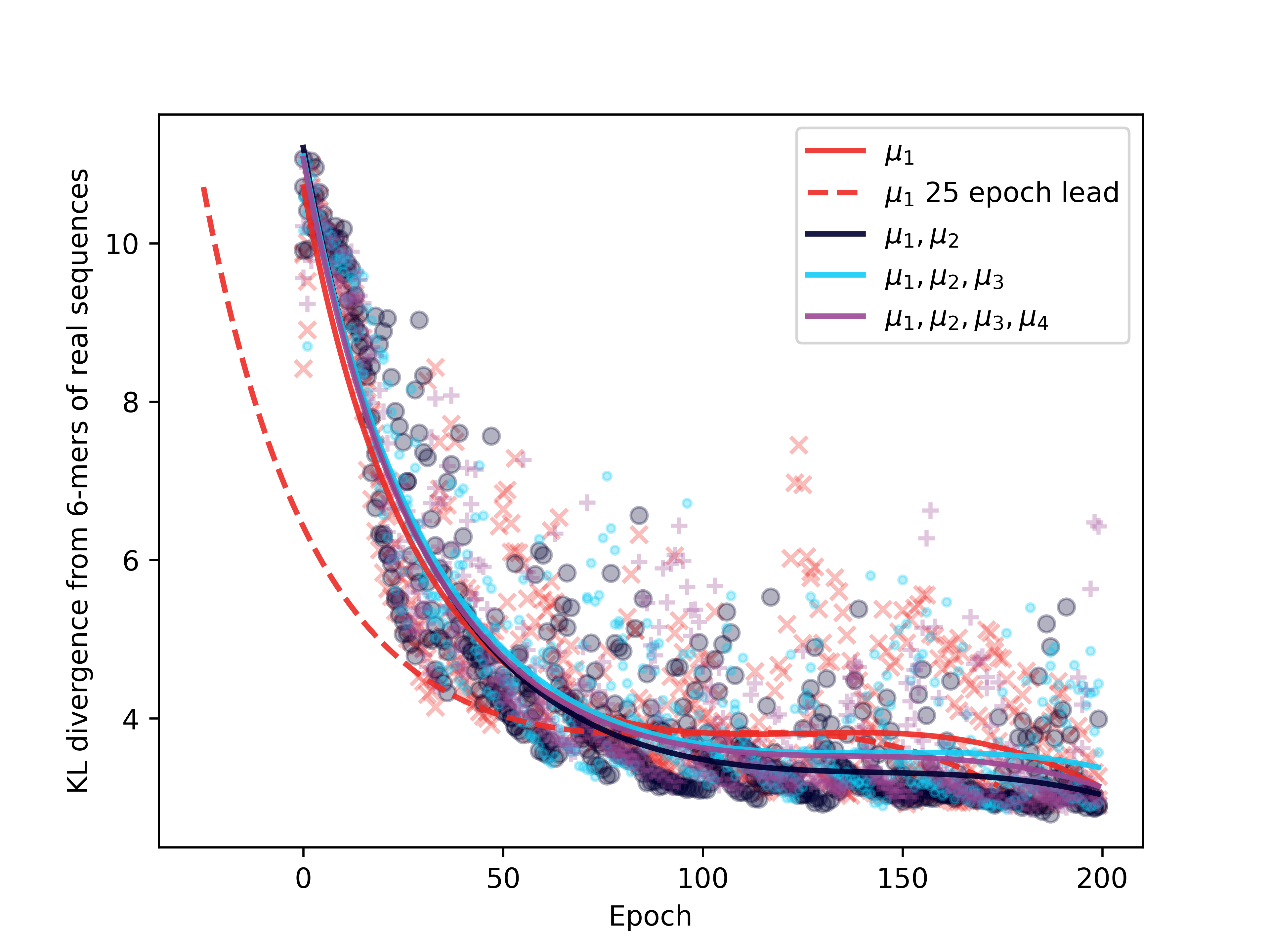
Figure 1: Sequence quality during training. A standard WGAN (with loss using only the first moment $\mu_{1}$) is compared to WGANs using further central moments $m\leq 4$. Each scatter data point represents an estimate of the post-epoch 6-mer KL divergence on $2\times 10^{4}$ sequences generated by $g$. Five replicate experiments are performed for each model, each is fit with a curve, and the aggregate of all curves is plotted. For reference, the dashed line plots the standard WGAN shifted 25 epochs early.

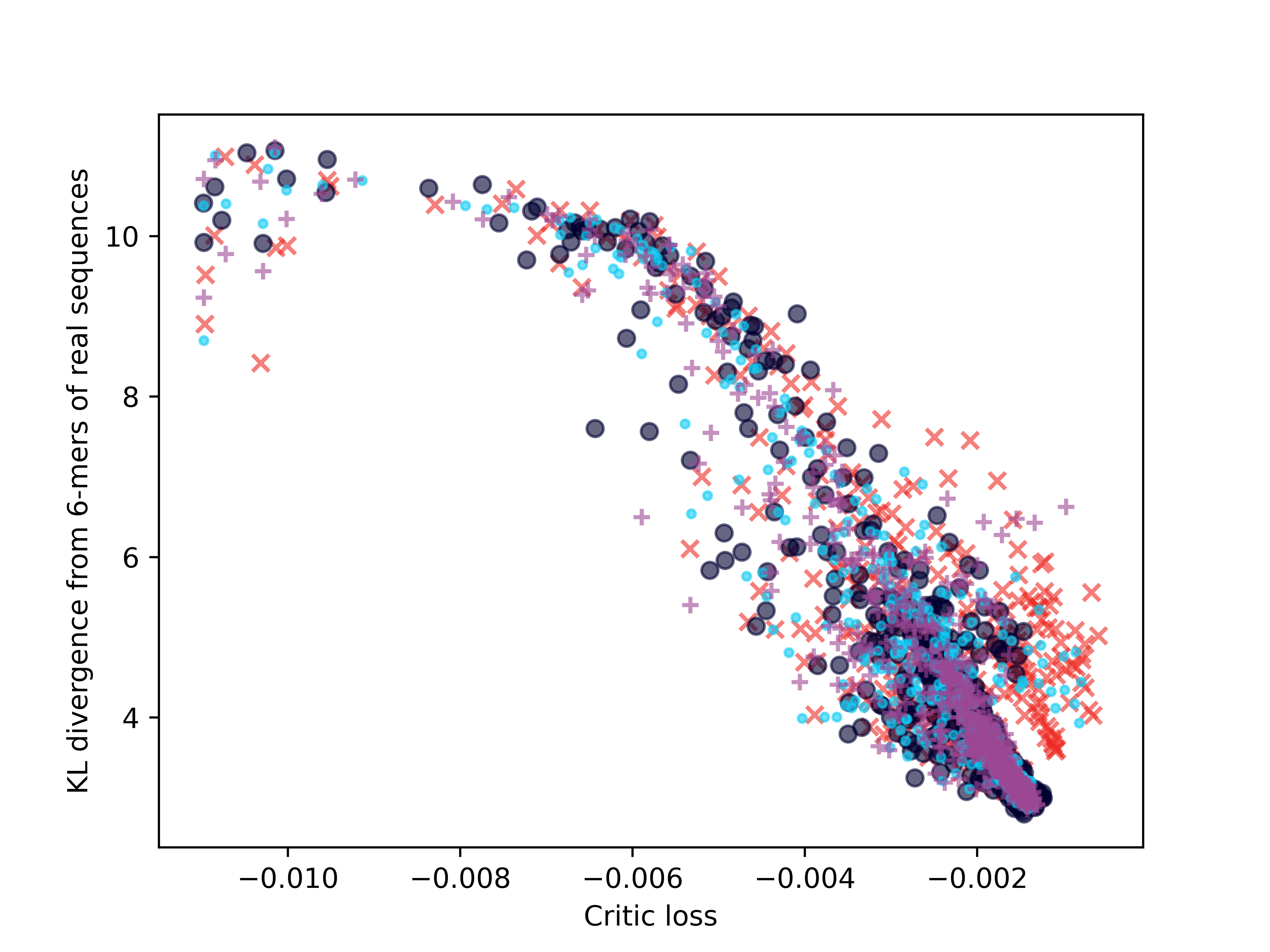
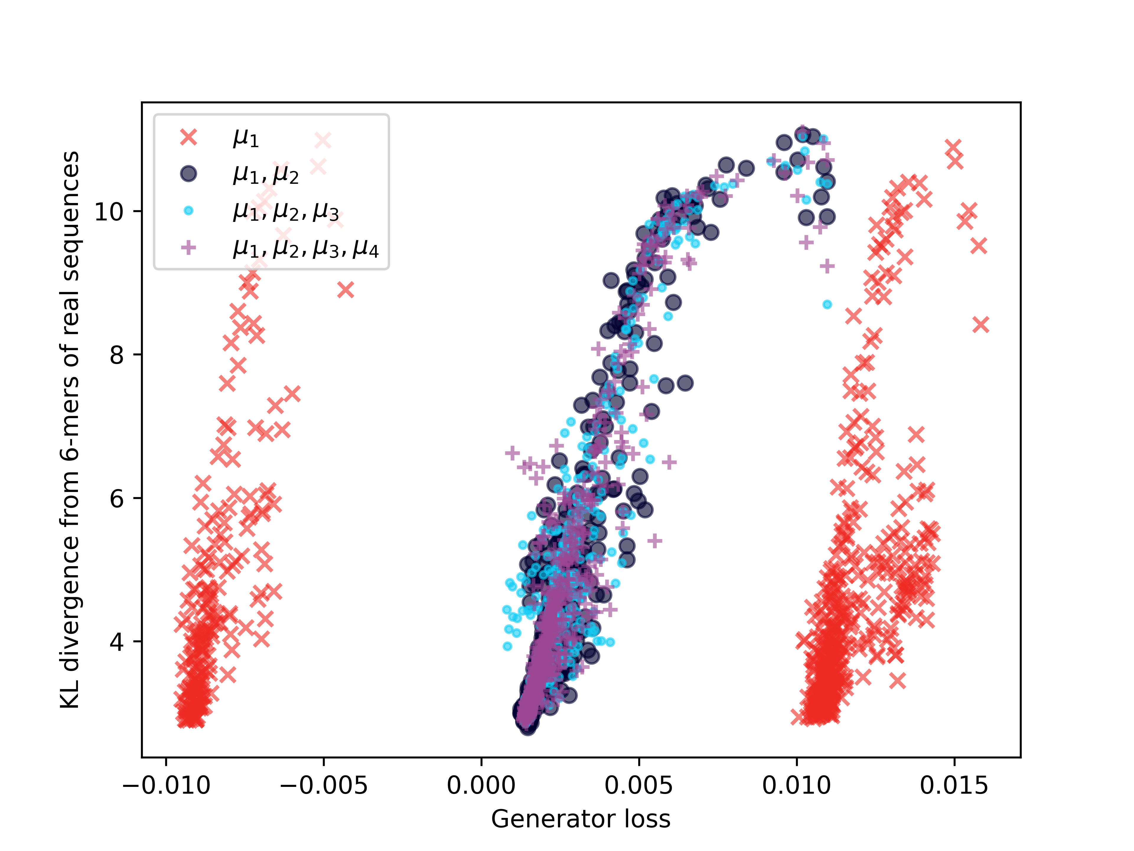
(a)	(b)

Figure 2: Quality of generator loss function throughout training. A standard WGAN (with loss using only the first moment $\mu_{1}$) is compared to WGANs using further central moments $m\in\{1,2,3,4\}$ using data obtained from Figure 1. The correspondence between the loss functions and the 6-mer KL divergence quantify the quality of the loss function as a surrogate for optimizing sequence quality. Critic loss is standard throughout, but is affected by generator training; generator loss varies with $m$. Loss functions are computed during training, and so include dropout and other stochastic effects.

$m$	Mean runtime (s)	KL & crit. loss $\rho$	KL & gen. loss $\rho$
1	2917.66	0.7059	0.4169
2	3079.00	0.8961	0.9257
3	3097.12	0.8388	0.8722
4	3110.64	0.8921	0.9205

Table 1: Runtime and quality of various generator loss functions. Standard WGAN loss with $m=1$ is compared to losses with higher moments $m>1$. Total 200 epoch runtime is averaged over five replicates. The Spearman rank correlation coefficient $\rho$ between each loss function and the 6-mer KL divergence is also displayed. Critic loss is standard throughout, but is affected by generator training. Generator loss varies $m\in\{1,2,3,4\}$. Loss functions are computed during training, and so include dropout and other stochastic effects.

4 Discussion

Figure 1 demonstrates that early in training, the standard WGAN exhibits superior performance; however, later on, using higher moments results in benefit to sequence quality, specifically for the $m=2$ and $m=4$ loss functions. This is shown to be rougly equivalent to gaining a 25 epoch advantage.

Figure 2 and Table 1 demonstrate a greater correspondence between sequence quality and loss functions with higher moments.

Qualitatively, using higher moments incentivizes optimizing batches as a whole. One way that this may manifest is by improving batch diversity of $\hat{x}$ to better match that of $x$, thereby reducing modal collapse. For early epochs, this could explain the slightly poorer performance, as these $m>1$ loss functions will initially be less seeking of a dominant nearby mode.

Interestingly, $m=3$ did not perform as well as $m=2$ and $m=4$. This could be because training the critic inherently drives $f$ toward a high-concentration similar to a Dirac delta. While the first moment $\mu_{1}$ is informative and even moments describe spread (variance $\mu_{2}$ quantifies spread, excess kurtosis $\mu_{4}$ quantifies modality near $\mu_{1}$), the skew, $\mu_{3}$, informs of direction but in a way that may here be less useful or numerically stable than simply using $\mu_{1}$.

Using higher moments increased runtimes, but not substantially. Training modified WGAN with $m=2$ moments in $g$’s loss required $<5.6\%$ more runtime than the standard WGAN. At a cost of $2.176 per hour[11], this corresponds to a cost of $1.76 per replicate of the standard WGAN, and less than $0.10 more expensive to train the $m=2$ variant; however, the $m=2$ variant reaches comparable convergence in 75% of the training, and thus would cost roughly $1.63 per replicate. For larger data and more stringent convergence criteria, the exponentially decaying gain in sequence quality by training for further epochs suggests that this 25 epoch advantage demonstrated by the $m>1$ variants would produce benefits far more dramatic. Furthermore, it is likely the benefits illustrated here would be stronger with more replicate experiments.

It is possible that deviations for different moments should receive their own weighting in computing the loss function. In this manner, it may be desirable to perform batch-based discrimination, where each batch is reduced to its constituent moments, and then a critic $f^{\prime}(\mu_{1},\mu_{2},\ldots\mu_{m})$ is computed on the moments $\mu_{1},\mu_{2},\ldots\mu_{m}$ of critic values $f$ for the batch. Parameters $\theta_{f^{\prime}}$ could be learned and clamped during training to ensure $\|f^{\prime}\|_{L}\leq 1$.

5 Conclusion

Here we have shown that viewing distributions with several moments rather than only using the first moment, $\mathbb{E}[f]$, improves WGAN training. We could also easily train the critic $f$ using this strategy.

6 Acknowledgements

Thank you to Ryan Emerson and Randolph Lopez for the scientific discussion, James Harrang for the helpful comments, and to the entire A-Alpha Bio team.

7 Declarations

7.1 Conflicts of interest

O.S. is an employee of A-Alpha Bio and owns stock options in the company.

References

- [1] Ian Goodfellow, Jean Pouget-Abadie, Mehdi Mirza, Bing Xu, David Warde-Farley, Sherjil Ozair, Aaron Courville, and Yoshua Bengio. Generative adversarial nets. Advances in neural information processing systems, 27, 2014.
- [2] Martin Arjovsky, Soumith Chintala, and Léon Bottou. Wasserstein generative adversarial networks. In International conference on machine learning, pages 214–223. PMLR, 2017.
- [3] John Thickstun. Kantorovich-Rubinstein Duality, 2019.
- [4] Leslie Greengard and Vladimir Rokhlin. A fast algorithm for particle simulations. Journal of computational physics, 73(2):325–348, 1987.
- [5] Julianus Pfeuffer and Oliver Serang. A bounded p-norm approximation of max-convolution for sub-quadratic bayesian inference on additive factors. The Journal of Machine Learning Research, 17(1):1247–1285, 2016.
- [6] Tileli Amimeur, Jeremy M Shaver, Randal R Ketchem, J Alex Taylor, Rutilio H Clark, Josh Smith, Danielle Van Citters, Christine C Siska, Pauline Smidt, Megan Sprague, et al. Designing feature-controlled humanoid antibody discovery libraries using generative adversarial networks. BioRxiv, 2020.
- [7] Aleksandr Kovaltsuk, Jinwoo Leem, Sebastian Kelm, James Snowden, Charlotte M Deane, and Konrad Krawczyk. Observed antibody space: a resource for data mining next-generation sequencing of antibody repertoires. The Journal of Immunology, 201(8):2502–2509, 2018.
- [8] Tobias H Olsen, Fergus Boyles, and Charlotte M Deane. Observed antibody space: A diverse database of cleaned, annotated, and translated unpaired and paired antibody sequences. Protein Science, 31(1):141–146, 2022.
- [9] John G Proakis. Digital signal processing: principles algorithms and applications. Pearson Education, 2001.
- [10] Diederik P Kingma and Jimmy Ba. Adam: A method for stochastic optimization. arXiv preprint arXiv:1412.6980, 2014.
- [11] Amazon EC2 G4 Instances, 8 2022. Archived at https://web.archive.org/web/20220809081441/https://aws.amazon.com/ec2/instance-types/g4/.