Vortex gap solitons in spin-orbit-coupled Bose-Einstein condensates with competing nonlinearities

Abstract

The formation and dynamics of full vortex gap solitons (FVGSs) is investigated in two-component Bose-Einstein condensates with spin-orbit coupling (SOC), Zeeman splitting (ZS), and competing cubic and quintic nonlinear terms, while the usual kinetic energy is neglected, assuming that it is much smaller than the SOC and ZS terms. Unlike previous SOC system with the cubic-only attractive nonlinearity, in which solely semi-vortices may be stable, with the vorticity carried by a single component, the present system supports stable FVGS states, with the vorticity present in both components (such states are called here “full vortex solitons”, to stress the difference from the half-vortices). They populate the bandgap in the system’s linear spectrum. In the case of the cubic self-attraction and quintic repulsion, stable FVGSs with a positive effective mass exist near the top of the bandgap. On the contrary, the system with cubic self-repulsion and quintic attraction produces stable FVGSs with a negative mass near the bottom of the bandgap. Mobility and collisions of FVGSs with different topological charges are investigated too.
Key words: Full vortex gap solitons, cubic-quintic nonlinearity, soliton dynamics

I Introduction

Since the Bose-Einstein condensates (BECs) have been created in ultracold gases of alkali metals Anderson1995 ; Bradley1995 ; Davis1995 , they have become a universal platform to study many phenomena in superfluids, such as vortices Williams1999 ; Kasamatsu2003 , solitons Burger1999 ; Anderson2001 and many other dynamical effects Heinzen2000 ; Morsch2006 ; Eckardt2009 . In their straightforward form, one-dimensional (1D) solitons stably exist in BECs without external traps, while two- and three-dimensional (2D and 3D) solitons are made unstable by the presence of the collapse, driven by the cubic self-attraction Berg1998 ; Sulem1999 ; Fibich2015 ; Malomed2005 ; Malomed2016 .

A significant direction in the work with atomic BEC is their use for emulation of various phenomena which are known in a much more complex form in condensed-matter physics emulator ; Ahufinger . In particular, synthetic spin-orbit coupling (SOC), which simulates this fundamental effect well known in physics of semiconductors Dresselhaus ; Bychkov , has been realized in two-component BEC by using counterpropagating Raman laser beams to engineer the necessary coupling between the two atomic states in the binary condensate Lin2011 ; Liu2014 ; Wu2016 . SOC is a source of many remarkable findings in BECs, including various extended patterns, vortices, and solitons Wang2010 ; Kawakami2011 ; Kawakami2012 ; Conduit2012 ; Liu2012 ; Zhou2013 ; Zezyulin2013 ; Sakaguchi2013 ; Xu2013 ; Kartashov2013 ; Kartashov2017 . A noteworthy fact is that SOC affects ground-state properties and enhances stability of the system, suppressing the critical collapse in the two-dimensional BEC with the self- and cross-attractive cubic nonlinearity, thus making it possible to predict absolutely stable 2D solitons Sakaguchi2014 ; Sakaguchi2016 . In 3D, full suppression of the respective supercritical collapse is not possible, but SOC was predicted to maintain metastable 3D solitons Zhang2015 . The 2D and 3D solitons created by SOC may be semi-vortices (SVs), built of zero-vorticity and vortical components, or mixed modes (MMs), which combine zero-vorticity and vortex terms in both components Sakaguchi2014 ; Zhang2015 ; Sakaguchi2016 ; Malomed2018 . In the context of binary dipolar BECs, SOC may support stable anisotropic 2D composite solitons Li2017 .

Under the action of strong Zeeman splitting (ZS) added to the SOC system, the MM states are transformed into stable SV gap solitons Sakaguchi2018 . The same effect stabilizes 2D solitons, supported by long-range dipole-dipole interactions between atoms carrying permanent magnetic moments, close to the edge of the ZS-induced bandgap Liao2017 . However, the dominant component of the 2D composite gap solitons, reported in Refs. Liao2017 and Sakaguchi2018 , is a fundamental mode without any phase structure. The creation of stable full-vortex gap solitons (FVGSs) in the SOC-affected BEC system, which, unlike the SVs, would carry vorticity in both components, remains a challenging problem. In fact, such solitons were considered, in the form of “excited states” of SVs and MMs, in the system which did not include the ZS terms Sakaguchi2014 . However, they all were found to be completely unstable states.

To construct stable FVGSs in this work, we use competing cubic and quintic nonlinearities. This approach is suggested by the prediction of robust 2D Li2018 ; Zhang2019 ; Lin2021 ; Zheng2021 and 3D Taruell vortex states in quantum droplets, which are stabilized by the Lee-Huang-Yang effect, i.e., additional quartic self-repulsive nonlinearity, induced by quantum fluctuations around mean-field states. The stability is provided by the competition of the quartic self-repulsion with the cubic mean-field attraction between components in the binary BEC Petrov2015 ; Petrov2016 ; Schmitt2016 ; Cabrera2018 . A similar possibility is to consider higher-order nonlinearities of the mean-field origin in BEC Yamaguchi1979 . In that connection, it is relevant to mention that, in addition to the common two-body (cubic) interaction, the three-body (quintic) term can be adjusted by means of the Feshbach resonance Marcelli1999 ; Smith2014 ; Adhikari2017 . In previous studies, it was demonstrated that competing cubic self-attraction and quintic repulsion could provide the stability of vortex solitons in BECs (in the absence of SOC) Mithun2013 ; Abdullaev2001 ; Gao2018 ; PhysicaD ; Xu2021 .

In this work, we consider a possibility to use the interplay of the competing nonlinearities, SOC, and ZS to support stable FVGSs in the two-component BEC system. We produce the density distribution and phase structure for families of stationary vortex solitons with different topological charges, and identify their stability. Their mobility and collisions are addressed too.

The paper is organized as follows. In Section 2, we introduce the model and FVGS states in it. In Section 3, we study the dynamics, mobility and collisions of the FVGSs by means of systematic simulations. The paper is concluded by Section 4.

II The model and stationary solutions

II.1 The coupled Gross-Pitaevskii equations

We consider the binary BEC which, in the mean-field approximation, is modelled by the system of 2D Gross-Pitaevskii equations (GPEs) for wave functions $\tilde{\psi}_{\pm}(\tilde{x},\tilde{y})$ of two components of the condensate. The equations include the Rashba-type SOC Rashba ; Sakaguchi2016 with strength $\lambda$, ZS with chemical-potential difference $2\tilde{\Omega}$ (both $\lambda$ and $\tilde{\Omega}$ are defined to be positive), and a combination of cubic and quintic terms, which represents two-body and three-body interactions, respectively Abdullaev2001 ; Braaten2002 ; Bulgac2002 ; Michinel1 ; Salerno ; Kofane :

$$i\hbar{\frac{\partial}{\partial\tilde{t}}}\tilde{\psi}_{\pm}=-{\frac{\hbar^{2}}{2m}}\nabla_{\pm}^{2}\tilde{\psi}\pm\lambda\left({\frac{\partial}{\partial\tilde{x}}}\mp i{\frac{\partial}{\partial\tilde{y}}}\right)\tilde{\psi}_{\mp}\mp\tilde{\Omega}\tilde{\psi}_{\pm}+g_{1}(|\tilde{\psi}_{\pm}|^{2}+|\tilde{\psi}_{\mp}|^{2})\tilde{\psi}_{\pm}+g_{2}(|\tilde{\psi}_{\pm}|^{2}+|\tilde{\psi}_{\mp}|^{2})_{\pm}^{2}\tilde{\psi}$$ (1)

(the tilde designates variables and coefficients which are replaced below by their scaled counterparts). The strength of the two-body interaction,

$$g_{1}=2\sqrt{2\pi}\hbar^{2}a/\left(a_{\perp}m\right),$$ (2)

is proportional to the s-wave scattering length $a$ ($a>0$ and $a<0$ represent the repulsive and attractive interactions, respectively), and inversely proportional to size $a_{\perp}$ of the confinement in the transverse direction Dalfovo1999 . The ZS effect can be induced by an artificial magnetic field in BECs, which breaks the symmetry between the two components of the binary wave function and produces a bandgap in the energy spectrum of the system Lin2011 ; Quay2010 ; Goldman2014 .

The nonlinearity in Eq. (1) is written in the Manakov’s form Manakov , i.e., with equal coefficients of the self- and cross-interactions, which is a relevant approximation for mixtures of two different atomic states Manakov-BEC ; Manakov-BEC2 . The magnitude and sign of $a$ can be adjusted to necessary values in Eq. (2) by means of the Feshbach resonance Feshbach . Further, the strength of the quintic nonlinearity is

$$g_{2}=\frac{4\sqrt{3}\hbar^{2}a^{4}}{ma_{\perp}^{2}}\left[d_{1}+d_{2}\tan\left(s_{0}\ln\frac{|a|}{|a_{0}|}+\frac{1}{2}\right)\right],$$ (3)

where $a_{0}$ is the value of $a$ at which a three-body bound state appears, $d_{1,2}$ and $s_{0}$ being coefficients given in Refs. Bulgac2002 ; Braaten2002 . It is known that $g_{2}$ can be tuned to arbitrary positive or negative value. In this work, we focus on the competition between the cubic and quintic nonlinearities with opposite signs, which implies $g_{1}g_{2}<0$. As mentioned above, the s-wave scattering length $a$ in Eq. (2) can be tuned to a desired value by means of the Feshbach-resonance technique, therefore the value of $g_{1}$ is also adjustable.

Following Refs. Li2017 and Sakaguchi2018 , we focus on the situation when the SOC energy is much larger than the kinetic energy, which implies the consideration of configurations with sufficiently large characteristic length scales, $l\gg\hbar^{2}/\left(m\lambda\right)$. In this case, terms $\sim\nabla^{2}\psi_{\pm}$ in Eq. (1) may be neglected. By means of scaling,

$$\tilde{\psi}_{\pm}=\sqrt{\left|g_{1}/g_{2}\right|}\psi_{\pm},\left(\tilde{x},\tilde{y}\right)=\left(\lambda\left|g_{2}\right|/g_{1}^{2}\right)\left(x,y\right),\tilde{t}=\left(\hbar\left|g_{2}\right|/g_{1}^{2}\right)t,\tilde{\Omega}=\left(g_{1}^{2}/\left|g_{2}\right|\right)\Omega,$$ (4)

the so simplified GPE system is cast in the following form, in which the nonlinearity and SOC coefficients are set to be $1$:

$$i{\frac{\partial}{\partial t}}\psi_{+}=\left({\frac{\partial}{\partial x}}-i{\frac{\partial}{\partial y}}\right)\psi_{-}-\Omega\psi_{+}-(|\psi_{+}|^{2}+|\psi_{-}|^{2})\psi_{+}+\left(|\psi_{+}|^{2}+|\psi_{-}|^{2}\right)^{2}\psi_{+},$$

$$i{\frac{\partial}{\partial t}}\psi_{-}=-\left({\frac{\partial}{\partial x}}+i{\frac{\partial}{\partial y}}\right)\psi_{+}+\Omega\psi_{-}-(|\psi_{-}|^{2}+|\psi_{+}|^{2})\psi_{-}+\left(|\psi_{-}|^{2}+|\psi_{+}|^{2}\right)^{2}\psi_{-},$$ (5)

in the case of the competition between cubic attraction and quintic repulsion, or

$$i{\frac{\partial}{\partial t}}\psi_{+}=\left({\frac{\partial}{\partial x}}-i{\frac{\partial}{\partial y}}\right)\psi_{-}-\Omega\psi_{+}+(|\psi_{+}|^{2}+|\psi_{-}|^{2})\psi_{+}-(|\psi_{+}|^{2}+|\psi_{-}|^{2})^{2}\psi_{+},$$

$$i{\frac{\partial}{\partial t}}\psi_{-}=-\left({\frac{\partial}{\partial x}}+i{\frac{\partial}{\partial y}}\right)\psi_{+}+\Omega\psi_{-}+(|\psi_{-}|^{2}+|\psi_{+}|^{2})\psi_{-}-(|\psi_{+}|^{2}+|\psi_{-}|^{2})^{2}\psi_{-},$$ (6)

in the opposite case of the cubic repulsion and quintic attraction. The remaining ZS parameter $\Omega$ may be also fixed by rescaling, but we keep it in the equations, as it is relevant to display some results for a fixed norm of the solution, while varying $\Omega$.

Actually, Eqs. (5) and (6) can be transformed into each other by simple substitution

$$\psi_{\pm}\rightarrow\psi_{\mp}^{\ast},$$ (7)

where $\ast$ stands for the complex conjugate; however, this transformation does not apply to the full system of Eqs. (1).

The linearization of Eqs. (5) and (6) is carried out by substituting

$$\psi_{\pm}=\varphi_{\pm}\exp\left(-i\omega t+ipx+iqy\right)$$ (8)

with constant amplitudes $\varphi_{\pm}$, which leads to the dispersion relation between the frequency $\omega$ and wave numbers $p$ and $q$ Li2017

$$\omega^{2}=\Omega^{2}+(p^{2}+q^{2}),$$ (9)

which is plotted in Fig. 1. Obviously, Eq. (9) with $\Omega\neq 0$ gives rise to the bandgap of width $2\Omega$, which may be populated by gap solitons.

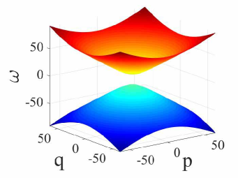
Figure 1: (Color online) Dispersion relation given by Eq. (9) with $\Omega=10$.

II.2 Stationary gap solitons existing at bottom and top edges of the bandgap.

Soliton solutions of Eqs. (5) and (6) with chemical potential $\mu$ are looked for as

$$\psi_{\pm}=e^{-i\mu t}\phi_{\pm}(x,y),$$ (10)

where $\phi_{\pm}$ are stationary wave functions. At the bottom and top edges of the bandgap, the chemical potential of the soliton is defined as

$$\mu=\begin{cases}\Omega-\Delta\mu,\quad&\mathrm{top}\text{ }\mathrm{of}\text{ }\mathrm{the}\text{ }\mathrm{bandgap,}\\ -\Omega+\Delta\mu,\quad&\mathrm{bottom}\text{ }\mathrm{of}\text{ }\mathrm{the}\text{ }\mathrm{bandgap,}\end{cases}$$ (11)

with

$$0<\Delta\mu<<\Omega.$$ (12)

The total norm of the two-component wave function, defined by

$$N=N_{+}+N_{-}\equiv\int\int\left[|\psi_{+}(x,y)|^{2}+|\psi_{-}(x,y)|^{2}\right]dxdy,$$ (13)

is a dynamical invariant of the system. The value of the norm is a natural characteristic of the solitons.

Below, we analyze the existence of the gap solitons in the edge regions which are defined as per Eq. (11). The analysis is presented here for Eq. (6), as, near the bottom and top edges of the bandgap Eq. (11), the transformation provided by Eq. (7) automatically produces solutions for the stationary wave functions $\phi_{\pm}$, defined as per Eq. (10) and Eq. (5):

$$\phi_{\mp}^{\mathrm{(top(stable);bottom(unstable))}}\left\{\mathrm{Eq.~{}}\text{(\ref{1})}\right\}=\left[\phi_{\pm}^{\mathrm{(bottom(stable);top(unstable))}}\left\{\mathrm{Eq.~{}}\text{(\ref{2})}\right\}\right]^{\ast}.$$ (14)

The Lagrangian of Eq. (6) is

$$\mathcal{L}=\int\int\left(\frac{i}{2}\sum_{+,-}\psi_{\pm}^{\ast}\frac{\partial\psi_{\pm}}{\partial t}+\mathrm{c.c.}\right)dxdy-H,$$ (15)

where $\mathrm{c.c.}$ stands for the complex-conjugate expression, and the Hamiltonian (another dynamical invariant of the system) is

$$H = \int\int\left\{\left[\frac{1}{2}\left(\psi_{+}^{\ast}\frac{\partial\psi_{-}}{\partial x}-i\psi_{+}^{\ast}\frac{\partial\psi_{-}}{\partial y}\right)+\mathrm{c.c.}\right]+\Omega\left(\left|\psi_{-}\right|^{2}-\left|\psi_{+}\right|^{2}\right)\right.$$ (16)

$$\left.+\frac{1}{2}\left(\left|\psi_{+}\right|^{2}+\left|\psi_{-}\right|^{2}\right)^{2}-\frac{1}{3}\left(\left|\psi_{+}\right|^{2}+\left|\psi_{-}\right|^{2}\right)^{3}\right\}dxdy.$$

The application of the Noether’s theorem Noether to Eq. (15) produces the conserved momentum in the same form as in Schrödinger equations, namely,

$$\mathbf{P}=i\int\int[\nabla(\psi_{+}^{\ast})\psi_{+}+\nabla(\psi_{-}^{\ast})\psi_{-}]dxdy.$$ (17)

On the other hand, the angular momentum, which may be conveniently written in terms of polar coordinates $\left(r,\theta\right)$ as

$$\Lambda=i\int_{0}^{\infty}rdr\int_{0}^{2\pi}d\theta\sum_{+,-}\frac{\partial\psi_{\pm}^{\ast}}{\partial\theta}\psi_{\pm},$$ (18)

is not conserved in the framework of the SOC system. Indeed, rewriting Eq. (6) in terms of $\left(r,\theta\right)$,

$$i{\frac{\partial}{\partial t}}\psi_{+}=e^{-i\theta}\left({\frac{\partial}{\partial r}}-\frac{i}{r}{\frac{\partial}{\partial\theta}}\right)\psi_{-}-\Omega\psi_{+}+(|\psi_{+}|^{2}+|\psi_{-}|^{2})\psi_{+}-(|\psi_{+}|^{2}+|\psi_{-}|^{2})^{2}\psi_{+},$$

$$i{\frac{\partial}{\partial t}}\psi_{-}=-e^{i\theta}\left({\frac{\partial}{\partial r}}+\frac{i}{r}{\frac{\partial}{\partial\theta}}\right)\psi_{+}+\Omega\psi_{-}+(|\psi_{-}|^{2}+|\psi_{+}|^{2})\psi_{-}-(|\psi_{+}|^{2}+|\psi_{-}|^{2})^{2}\psi_{-},$$ (19)

one obtains

$$\frac{d\Lambda}{dt}=2\int_{0}^{\infty}rdr\int_{0}^{2\pi}d\theta~{}\mathrm{Im}\left(e^{i\theta}\psi_{+}\frac{\partial\psi_{-}^{\ast}}{\partial r}\right).$$ (20)

Substituting Eq. (10) into Eq. (6) yields the following equations:

$$\mu\phi_{+}=\left({\frac{\partial}{\partial x}}-i{\frac{\partial}{\partial y}}\right)\phi_{-}-\Omega\phi_{+}+(|\phi_{+}|^{2}+|\phi_{-}|^{2})\phi_{+}-\left(|\phi_{+}|^{2}+|\phi_{-}|^{2}\right)^{2}\phi_{+},$$

$$\mu\phi_{-}=-\left({\frac{\partial}{\partial x}}+i{\frac{\partial}{\partial y}}\right)\phi_{+}+\Omega\phi_{-}+(|\phi_{-}|^{2}+|\phi_{+}|^{2})\phi_{-}-\left(|\phi_{-}|^{2}+|\phi_{+}|^{2}\right)^{2}\phi_{-}.$$ (21)

In particular, near the bottom edge of the bandgap, which is defined as per the bottom line of Eq. (11), the first equation of Eq. (21) amounts, in the lowest approximation, to a linear relation (cf. Ref. Sakaguchi2016 ),

$$\phi_{-}\approx\left(2\Omega\right)^{-1}\left({\frac{\partial}{\partial x}}+i{\frac{\partial}{\partial y}}\right)\phi_{+}.$$ (22)

Substituting this in the first equation of Eq. (21), one obtains

$$-\Delta\mu\cdot\phi_{+}=-\left(2\Omega\right)^{-1}\left({\frac{\partial^{2}}{\partial x^{2}}}+{\frac{\partial^{2}}{\partial y^{2}}}\right)\phi_{+}-|\phi_{+}|^{2}\phi_{+}+|\phi_{+}|^{4}\phi_{+}.$$ (23)

This equation, which combines the effective cubic self-attraction and quintic repulsion, has a chance to produce stable 2D solitons Michinel2 ; Berntson . It is well known that such solitons, with all values of the embedded vorticity (winding number), exist in interval Bulgaria ; Canada ; Berntson

$$0<\Delta\mu<3/16,$$ (24)

with the respective values of the norm

$$N(\Delta\mu\rightarrow 0)\rightarrow 0,N\left(\Delta\mu\rightarrow 3/16\right)\rightarrow\infty.$$ (25)

Near the top edge of the bandgap, defined as per the top line of Eq. (11), approximate relation (22) is replaced by one following from the second equation of Eq. (21):

$$\phi_{+}\approx{\frac{1}{2\Omega}}\left({\frac{\partial}{\partial x}}-i{\frac{\partial}{\partial y}}\right)\phi_{-}.$$ (26)

Substituting it into the second equation of Eq. (21), one obtains

$$-\Delta\mu\cdot\phi_{-}=-{\frac{1}{2\Omega}}\left({\frac{\partial^{2}}{\partial x^{2}}}+{\frac{\partial^{2}}{\partial y^{2}}}\right)\phi_{-}+|\phi_{-}|^{2}\phi_{-}-|\phi_{-}|^{4}\phi_{-},$$ (27)

cf. Eq. (23). It is obvious that this equation, which combines the nonlinear terms with the signs opposite to those in Eq. (23), i.e., cubic self-repulsion and quintic attraction, may produce only unstable 2D solitons, which are subject to the destructive effect of the supercritical collapse.

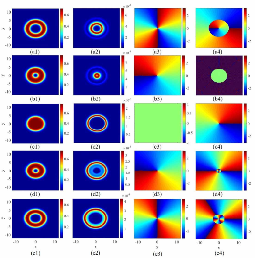
Figure 2: (Color online) Density patterns, $|\phi_{+}\left(x,y)\right)|^{2}$ and $|\phi_{-}\left(x,y\right)|^{2}$ (the first and second columns, respectively), and phase distributions in $\phi_{+}\left(x,y\right)$ and $\phi_{-}\left(x,y\right)$ (the third and fourth columns, respectively) for the two components of stable solitons located near the bottom edge of the bandgap, see Eq. (11), as produced by the numerical solution of Eq. (21). Values of the winding numbers of the components, from top to bottom, are: $(S_{+},S_{-})=(-2,-1)$, $(-1,0)$, $(0,1)$, $(1,2)$, and $(2,3)$. In all the panels, we fix the total norm as $N=50$ (see Eq. (13), and the ZS strength is $\Omega=5$.

III Numerical results

III.1 Stationary solutions for the vortex gap solitons

The analysis presented in the previous section indicates that stable stationary solutions for gap solitons may exist near the bottom edge of the bandgap produced by Eq. (6) or, according to Eqs. (7) and (14), near the top edge in the case of Eq. (5). The initial guess for solutions of stationary Eq. (21) was obtained by means of the imaginary-time method, applied to the time-dependent version of Eq. (23). Then, iterating the initial solution in the framework of the power-conserved squared-operator method Yang , stationary solutions were produced in the numerically accurate form. Lastly, stability of the soliton solutions was tested by real-time simulations of Eq. (6), running from $t=0$ to $1000$. Actually, this is a very long time, which corresponds, roughly, to $\sim 1000$ solitons’ relaxation time, thus making conclusions about the stability of the stationary states fully reliable.

Note that the topological charges (winding numbers) of two components of the stationary solitons are subject to a simple relation Sakaguchi2014 [the same relation follows from Eq. (26)],

$$S_{+}=S_{-}-1.$$ (28)

Typical examples of the numerically constructed stable stationary solution for the solitons, located close to the bottom edge of the bandgap, with $(S_{+},S_{-})=(-2,-1),(-1,0),(0,1),(1,2)$ and $(2,3)$, are displayed in Fig. 2. In particular, all the two-component modes in which both $S_{\pm}$ are different from zero represent FVGSs. Thus, these composite modes may indeed be stable, unlike their completely unstable counterparts in the form of “excited states”, in the usual SOC system with the cubic self-attraction Sakaguchi2014 . Further, Fig. 2 shows that component $\phi_{+}$ gives a dominant contribution to norm Eq.(13), while $\phi_{-}$ plays a subordinate role (i.e., $N_{-}\ll N_{+}$, ), being mainly distributed along the inner rim of $\phi_{+}$ in the case of $|S_{+}|>|S_{-}|$, or along the outer rim in the opposite case, $|S_{+}|<|S_{-}|$. For the FVGS modes located near the top edge of the bandgap, Eq. (26) indicates that $\phi_{-}$ plays a dominant role, while $\phi_{+}$ is a subordinate component $N_{-}\gg N_{+}$, which is mainly distributed along the inner or outer rim of $\phi_{-}$ for $|S_{+}|<|S_{-}|$ or $|S_{+}|>|S_{-}|$, respectively.

Characteristics of these soliton families are summarized in Fig. 3, in which we plot the shift of the chemical potential, $\Delta\mu$, defined as per the bottom line of Eq. (11), and the effective area of the soliton’s dominant component ($\phi_{\mathrm{d}}$),

$$A\equiv\frac{\left(\int\int|\phi_{\mathrm{d}}\left(x,y\right)|^{2}dxdy\right)^{2}}{\int\int|\phi_{\mathrm{d}}\left(x,y\right)|^{4}dxdy},$$ (29)

versus the total norm $N$ and ZS strength $\Omega$. Note that $\Delta\mu$ in panels (a) and (c) of the figure varies precisely in interval Eq. (24), in agreement with limit relations (25). The figure shows that there are two threshold values for $N$ and $\Omega$, namely, $N^{\mathrm{c1,c2}}$ and $\Omega^{\mathrm{c1,c2}}$, with $N^{\mathrm{c1}}<N^{\mathrm{c2}}$ and $\Omega^{\mathrm{c1}}<\Omega^{\mathrm{c2}}$. When $N<N^{\mathrm{c1}}$ or $\Omega<\Omega^{\mathrm{c1}}$, no soliton solutions are found, only spatially uniform states being possible; note that $N^{\mathrm{c1}}=\Omega^{\mathrm{c1}}=0$ for $S_{+}=0$ [these findings agree with the known fact that 2D vortex-soliton solutions of Eq. (23) exist if their norm exceeds a certain threshold value, while there is no existence threshold for zero-vorticity solutions Michinel2 . In intervals $N^{\mathrm{c1}}<N<N^{\mathrm{c2}}$ and $\Omega^{\mathrm{c1}}<\Omega<\Omega^{\mathrm{c2}}$, soliton solutions can be found, but they are unstable (as shown by dashed and dotted curves in Fig. 3). Finally, stable solutions exist at $N>N^{\mathrm{c2}}$ and $\Omega>\Omega^{\mathrm{c2}}$. These conclusions for the 2D cubic-quintic system are different from the case of its counterpart with the cubic-only nonlinearity, where the SV solutions with $S_{+}=0$, $S_{-}=1$ [see Eq. (28)] are stable in the entire bandgap Sakaguchi2016 .

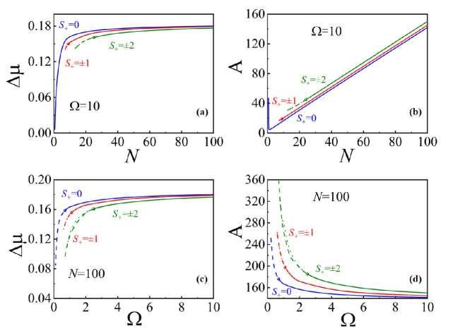
Figure 3: (Color online) The chemical-potential shift, defined as per Eq. (11), and the effective area of the dominant component, defined as per Eq. (29), versus the total norm $N$, at a fixed value of the ZS strength $\Omega$ (a,b), and versus $\Omega$ at a fixed value of $N$ (c,d). The results are produced by the numerical solution of Eq. (21). Blue, red and green curves represent the dependences for the soliton families with the vorticity in the dominant component $S_{+}=0$, $\pm 1$ and $\pm 2$, respectively, while the vorticity in the other component is given by Eq. (28). Solid curves represent stable branches, which correspond to $N>N^{\mathrm{c2}}$ and $\Omega>\Omega^{\mathrm{c2}}$ (see the text). These stability boundaries are designated by color balls on the curves. Dashed and dotted curves represent unstable branches, at $N<N^{\mathrm{c2}}$ and $\Omega<\Omega^{\mathrm{c2}}$ (the dashed curves pertain to $S_{+}=0$, $-1$ and $-2$, and the dotted ones correspond to $S_{+}=+1$ and $+2$. The stability of identified by means of systematic simulations of Eq. (6).

III.2 Mobility of the gap solitons initiated by kicking

Construction of moving solitons in the framework of Eqs. (5) and (6) is a nontrivial problem, as they are not Galilean invariant equations. We have studied the mobility in direct simulations via Eqs. (5) and (6), respectively, by applying kick $\eta$ to the stationary solution in the $x$ or $y$ direction. According to the relationship in Eq. (14), the corresponding inputs are defined as

$$\psi_{\pm}(x,y,t=0)=\begin{cases}\phi_{\mp}^{\ast}(x,y)\{e^{i\eta x},e^{i\eta y}\}&\mathrm{for\quad Eq.(\ref{1}),}\\ \phi_{\pm}(x,y)\{e^{i\eta x},e^{i\eta y}\}&\mathrm{for\quad Eq.(\ref{2}).}\end{cases}$$ (30)

The substitution of these expressions in Eq. (17) yields the respective values of the momentum produced by the kick,

$$P_{x,y}=N\eta.$$ (31)

For convenience, we name stable solutions of Eq. (5), which are located near the top edge of the bandgap, as “top-type solitons”, while the stable solutions of Eq. (6), which are located near the bottom edge of the bandgap, are named as “bottom-type solitons”.

Figure 4: (Color online) Motion of the soliton at the bottom (a1,a2) and top (b1,b2) of the bandgap initiated by kick $\eta=0.1$ in the positive $y$ direction, see Eq. (30). The first row is the motion of the soliton located near the bottom of the bandgap, with parameters $(N_{+},S_{+},\Omega)=(50,1,10)$. The second row is the same for the soliton located close to the top of the bandgap, with $(N_{-},S_{-},\Omega)=(50,1,10)$.

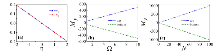
Figure 5: (Color online) (a) The velocity of the gap soliton, which is kicked along the positive $x$ (red) or $y$ (blue) direction, according to Eq. (30), versus $\eta$. The velocity is found numerically as per Eqs. (32) and (33) The soliton is taken near the bottom of the bandgap, with $(N_{+},S_{+},\Omega)=(50,0,10)$. (b) The effective mass of the solitons located near the top and bottom of the bandgap (short-dashed and dashed lines, respectively) versus the ZS strength, $\Omega$. Parameters of the solitons located near the bottom and top edges of the bandgap types are selected as $(N_{\pm},S_{\pm},\eta)=(50,0,0.1)$. (c) The effective mass of the solitons located near the top and bottom of the bandgap (short-dashed and dashed lines, with $(\Omega,S_{\pm},\eta)=(10,0,0.1)$, respectively) versus the total norm $N$. The masses are found as per Eq. (34).

Figure 4 displays cross-sections of the two components of the moving solitons located close to the bottom (a1,a2) and top (b1,b2) of the bandgap, applying $\eta=0.1$ in the positive $y$ direction, as per Eq. (30). The figure shows that the solitons in these two cases (for the solitons close to the bottom and top of bandgap) move steadily along the $y$ directions, which indicates that they have a negative and positive effective mass, respectively. The signs of the effective mass at the two edges of the bandgap are consistent with previous results Li2017 .

To accurately identify the effective mass of the solitons from the numerical data, as the ratio of momenta given by Eq. (31) [see Eq. (17)] to the corresponding velocities $V_{x,y}$, the center-of-mass (COM) coordinate of the soliton’s dominant component is calculated as

$$\{X_{\mathrm{COM}}(t),Y_{\mathrm{COM}}(t)\}=\frac{\int\int\{x,y\}|\psi_{\mathrm{d}}(x,y,t)|^{2}dxdy}{\int\int|\psi_{\mathrm{d}}(x,y,t)|^{2}dxdy}.$$ (32)

Then, the velocity is found as

$$V_{x}=[X_{\mathrm{COM}}(t)-X_{\mathrm{COM}}(0)]/t,\quad V_{y}=[Y_{\mathrm{COM}}(t)-Y_{\mathrm{COM}}(0)]/t.$$ (33)

Eventually, effective masses are obtained from here as

$$M_{x,y}=\frac{P_{x,y}}{V_{x,y}}\equiv\frac{N\eta}{V_{x,y}}.$$ (34)

The result, $V_{x}=V_{y}$, as displayed in Fig. 5(a), implies that, naturally, the effective mass is isotropic in the present system, i.e., $M_{x}=M_{y}$. Figs. 5(b,c) show that, as mentioned above, the solitons located near the bottom and top edges of the bandgap have negative and positive effective masses, respectively. Moreover, the numerical results, displayed in these figures, demonstrate that the effective masses linearly depend on $\Omega$ and $N$, and do not depend on winding numbers $S_{\pm}$. The increase of the masses with the increase of the ZS strength, $\Omega$, is explained by the fact that gap solitons do not exist at $\Omega=0$. The linear dependence of the masses on $N$ is a common property of solitons in models of the GPE type.

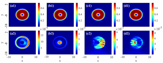
Figure 6: (Color online) The density distribution in the moving solitons kicked in the positive $y$ direction with different values of $\eta$ as per Eq. (30). The first and second rows display the dominant and subordinate components, respectively. Parameters of the soliton in panels (a1,a2,c1,c2) are $(N_{+},S_{+},\Omega)=(50,1,10)$, while for the soliton in panels (b1,b2,d1,d2) they are $(N_{+},S_{+},\Omega)=(50,-1,10)$. The first and second columns display the solitons kicked with $\eta=0.1$ and measured at $t=800$, while the third and fourth columns pertain to the solitons kicked with a kick which is ten times as large, therefore the data are taken at time which is ten times smaller, $t=80$.

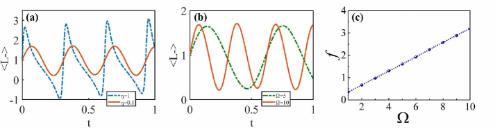
Figure 7: (Color online) (a) NOAM of the subordinate component of the soliton of the bottom-edge type versus $t$ for different values of the kick, i.e., $\eta=0.1$ and $1$ (the red solid and blue dashed curves, respectively). Parameters of the soliton are $(N_{+},S_{-},\Omega)=(50,1,10)$. (b) NOAM of a moving soliton with $(N_{+},S_{-},\eta)=(50,1,0.1)$ and different values of the ZS strength, i.e., $\Omega=5$ and $10$ (the green dashed and red solid curves, respectively). (c) The oscillation frequency of the NOAM of the subordinate component versus $\Omega$. Here, we also select the bottom-edge type of the soliton, with parameters $(N_{+},S_{+},\eta)=(50,0,0.1)$.

Typical examples of the density distribution in the solitons set in motion by the kick with different values of $\eta$ are shown, for the solitons taken near the bottom edge of the bandgap, in Fig. 6. The snapshots are taken at the moment of time when the COM of the soliton kicked in the $y$ direction is located at $y\approx 8$. It is observed that the dominant component of the moving solution ($\phi_{+}$, in the present case) maintains its shape, while the subordinate component, $\phi_{-},$ exhibits a deformation, as a consequence of the absence of the Galilean invariance in the system. Accordingly, in the case of a small kick $\eta$, the density distribution of the subordinate component is still confined within the main body of the moving soliton, see Figs. 6(a2,b2). In contrast, at large $\eta$, the subordinate components is lagging behind the main body of the soliton, which gives rise to its gradual delocalization, see Figs. 6(c2,d2).

In the case of small $\eta$, the subordinate component shows an asymmetric density distribution and rotates around the COM in the course of the direct simulations of the motion. This fact explains density oscillations in the cross-section diagram in Figs. 4(a2,b1). To characterize the motion of the soliton, we define the normalized orbital angular momentum (NOAM) of the two components as

$$\ \left\langle L_{\pm}\right\rangle=\frac{\int\psi_{\pm}^{\ast}\hat{L}\psi_{\pm}d\mathbf{r}}{N_{\pm}},$$ (35)

where $\hat{L}=-i(x\partial_{y}-y\partial_{x})$ is the angular-momentum operator. The direct simulations show that the NOAM of the dominant component stays nearly constant in the course of the motion, while the NOAM of the subordinate one oscillates as a function of $t$. For small $\eta$, the variation of $\left\langle L_{-}(t)\right\rangle$ manifests itself as harmonic oscillations [see the red curve in Fig. 7(a)], while for large $\eta$, the oscillations of $\left\langle L_{-}(t)\right\rangle$ are anharmonic due to the above-mentioned trend to delocalization of the density distribution, see the blue dashed curve in Fig. 7(a). Figure 7(b) displays the harmonic oscillations of $\left\langle L_{-}(t)\right\rangle$ for different values of $\Omega$. Further, the numerical results show that the frequency of the harmonic oscillations linearly depends on the ZS strength $\Omega$ for a fixed value of the norm of the subordinate component, see Fig. 7(c). On the other hand, the oscillation frequency does not depend on the winding number. Because the frequency of the harmonic oscillation is determined by the oscillator’s mass, the conclusion is the same as produced above on the basis of different numerical data in Fig. 5(b): the effective mass of the soliton linearly grows with $\Omega$, but it does not depend on the topological charge of the soliton.

III.3 Collisions between moving gap solitons

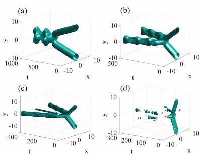
Figure 8: (Color online) Collisions of fundamental solitons (ones with $S_{+}=0$). Panels feature the collisions between the solitons set in motion as per Eq. (37) with (a) $\eta=0.1$, (b) $\eta=0.5$, (c) $\eta=0.9$, and (d) $\eta=3$. Here, parameters of the gap solitons are selected as $(N_{+},\Omega)=(10,10)$.

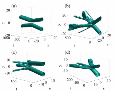
Figure 9: (Color online) Parameters of the colliding FVGSs in this figure are selected as $(N_{+},\Omega)=(20,10)$. (a,b) The colliding gap solitons have the same topological charge, with $S_{+}=1$. (a) An elastic collision between two gap solitons with $\eta=0.1$. (b) An inelastic collision with $\eta=0.7$. (c,d) Collisions of the solitons with opposite topological charges, $S_{+}=\pm 1$. The kick corresponding to Eq. (37) is $\eta=0.1$ in (c), and $\eta=0.7$ in (d).

A straightforward possibility is to simulate collisions between solitons which are set in motion by opposite kicks $\pm\eta$. For the solitons located near the bottom and top edges of the bandgap, we define the respective initial wave functions as

$$\psi_{\pm}(x,y,t=0)=\phi_{\pm}(x,y+y_{0})e^{-i\eta y}+\phi_{\pm}(x,y-y_{0})e^{i\eta y},$$ (36)

and

$$\psi_{\pm}(x,y,t=0)=\phi_{\pm}(x,y+y_{0})e^{i\eta y}+\phi_{\pm}(x,y-y_{0})e^{-i\eta y},$$ (37)

where $2y_{0}$ is the initial separation between the solitons. Due to the symmetry provided by Eq. (14), we here consider only the collision between the solitons of the bottom-edge type.

Figures 8 and 9 display several typical examples of collisions between the fundamental solitons and FVGSs, with different values of $\eta$, which are displayed by the contour surface of the density of the dominant component. In Fig. 8(a), a completely inelastic collision is observed for a small value of $\eta$, with the colliding fundamental solitons merging into a breather. On the contrary, in Fig. 8(b) a “twisted” quasi-elastic collision is observed for a moderate value of $\eta$: the colliding fundamental solitons first merge and then separate into ones moving perpendicular to the initial direction. It is further shown in Fig. 8(c) that three fragments appear after the collision when $\eta$ is large, a new fragment being a small-amplitude breather. Finally, it is shown in Fig. 8(d) that the solitons are completely destroyed by the collision if $\eta$ is sufficiently large.

The collision between two vortex solitons (FVGSs) shows different dynamics. In Figs. 9(a,b), the colliding solitons have identical topological charges, $S_{+}=1$. When $\eta$ is small, the solitons repel each other and maintain their shapes after the rebound, i.e., they collide elastically. In contrast, in the case of opposite topological charges, the colliding solitons also repel each other, but the outcome is different: they split into four fragments, as shown in Fig. 9(c).

When $\eta$ is large, the collisions of the vortex solitons are always inelastic. In the case of identical topological charges, collision-generated fragments are hurled in all directions, see Fig. 9(b). In the case of opposite topological charges, three fragments are generated by the collision, see Fig. 9(d). If $\eta$ is sufficiently large, the colliding FVGSs are completely destroyed by the collision. The latter case is not shown here.

Thus, the present system, based on Eq. (6), which is dominated by the SOC energy demonstrates the behavior completely different from what is common for usual models with the domination of the kinetic energy: collisions with large values of velocities tend to be destructive, rather than quasi-elastic.

IV Conclusions

In this work, we have investigated the formation of stable FVGSs (full-vortex gap solitons) and their dynamics in the two-component BEC with SOC (spin-orbit coupling) and competing cubic and quintic interactions. The difference from the previously studied 2D solitons in the SOC system with the cubic attractive interactions is that they might be stable solely in the SV (semi-vortex) form, with the vorticity carried by a single component. When the SOC and ZS (Zeeman-splitting) terms are sufficiently strong, the kinetic-energy ones may be neglected in the system of coupled GPEs (Gross-Pitaevskii equations). The so simplified system maintains a bandgap in its linear spectrum, populated by FVGSs. They may be stable near edges of the bandgap. If the absolute values of the topological charge of the dominant component is larger than that of the secondary one, the density distribution of the secondary component is surrounded by that of the dominant component. Otherwise, the dominant component is surrounded by the secondary one. We represent FVGS families by displaying dependences of the chemical potential and solitons’ effective area on the norm and ZS strength. The results reveal stability boundaries for the families. The mobility of the FVGSs is explored by kicking the stationary solitons. It is thus found that the FVGSs formed near the top and bottom edges feature, respectively, positive and negative dynamical masses. For a small kick, the minor component of solitons oscillates with the frequency proportional to the ZS strength. In contrast, under the action of a larger kick the minor suffers strong deformation, eventually leading to delocalization of the kicked soliton. Collisions between FVGSs with identical and opposite topological charges were considered too, featuring both elastic and inelastic outcomes.

A natural direction to extend the present work is to investigate self-trapped modes of the FVGSs type in a system with long-range dipole-dipole interactions, as well as in three-dimensional systems.

- (1) Anderson MH, Ensher JR, Matthews MR, Wieman CE, Cornell EA. Observation of Bose-Einstein condensation in a dilute atomic vapor. Science 1995;269:198.
- (2) Bradley CC, Sackett CA, Tollett JJ, Hulet RG. Evidence of Bose-Einstein condensation in an atomic gas with attractive interactions, Phys Rev Lett 1995;75:1687; Erratum: Phys Rev Lett 1997;79:1170.
- (3) Davis KB, Mewes MO, Andrews MR, van Druten NJ, Durfee DS, Kurn DM, Ketterle W. Bose-Einstein condensation in a gas of sodium atoms. Phys Rev Lett 1995;75:3969.
- (4) Williams JE, Holland MJ. Preparing topological states of a Bose-Einstein condensate. Nature 1999;401:568.
- (5) Kasamatsu K, Tsubota M, Ueda M. Vortex phase diagram in rotating two-component Bose-Einstein condensates. Phys Rev Lett 2003;91:150406.
- (6) Burger S, Bongs S, Dettmer S, ErtmerW, Sengstock K. Dark solitons in Bose-Einstein condensates. Phys Rev Lett 1999;83:5198.
- (7) Anderson BP, Haljan PC, Regal CA, Feder DL, Collins LA, Clark CW, Cornell EA. Watching dark solitons decay into vortex rings in a Bose-Einstein condensate. Phys Rev Lett 2001;86:2926.
- (8) Heinzen DJ, Wynar R, Drummond PD, Kheruntsyan KV. Superchemistry: Dynamics of coupled atomic and molecular Bose-Einstein condensates. Phys Rev Lett 2000;84:5029.
- (9) Morsch O, Oberthaler M. Dynamics of Bose-Einstein condensates in optical lattices. Rev Mod Phys 2006;78:179.
- (10) Eckardt A, Holthaus M, Lignier H, Zenesini A, Ciampini O, Morsch O, Arimondo E. Exploring dynamic localization with a Bose-Einstein condensate. Phys Rev A 2009;79:013611.
- (11) Bergé L. Wave collapse in physics: Principles and applications to light and plasma waves. Phys Rep 1998;303:259-370.
- (12) Sulem C, Sulem PL. Nonlinear Schrödinger Equations: Self-focusing Instability and Wave Collapse. New York: Science & Business Media; 2007.
- (13) Fibich G. The Nonlinear Schrödinger Equation: Singular Solutions and Optical Collapse. Berlin: Heidelberg; 2015.
- (14) Malomed BA, Mihalache D, Wise F and Torner L. Spatiotemporal optical solitons. J Opt B: Quantum Semiclass Opt 2005;7:R53-R72.
- (15) Malomed BA. Multidimensional solitons: Well-established results and novel findings. Eur Phys J Special Topics 2016;225:2507.
- (16) Hauke P, Cucchietti F M, Tagliacozzo L, Deutsch I, Lewenstein M. Can one trust quantum simulators? Rep Prog Phys 2012;75:082401.
- (17) Lewenstein M, Sanpera A, Ahufinger V. Ultracold Atoms in Optical Lattices: Simulating Quantum Many-Body Systems. Oxford: Oxford University Press;2012.
- (18) Dresselhaus G. Spin-orbit coupling effects in zinc blende structures. Phys Rev 1955;100:580-586.
- (19) Bychkov YuA, Rashba EI. Oscillatory effects, the magnetic susceptibility of carriers in inversion layers. J Phys C: Solid State Phys 1984;17:6039-6045.
- (20) Lin YJ, Jiménez-García K, Spielman IB. Spin-orbit-coupled Bose-Einstein condensate. Nature 2011;471:83.
- (21) Liu XJ, Law KT, Ng T K. Realization of 2D spin-orbit interaction and exotic topological orders in cold atoms. Phys Rev Lett 2014;112:086401.
- (22) Wu Z, Zhang L, Sun W, Xu XT, Wang BZ, Ji SC, Deng YJ, Liu XJ, Pan JW. Realization of two-dimensional spin-orbit coupling for Bose-Einstein condensates. Science 2016;354:83-88.
- (23) Kawakami T, Mizushima T, Nitta M, Machida K. Stable skyrmions in SU(2) gauged Bose-Einstein condensates. Phys Rev Lett 2012;109:015301.
- (24) Liu CF, Liu WM. Spin-orbit-coupling-induced half-skyrmion excitations in rotating and rapidly quenched spin-1 Bose-Einstein condensates. Phys Rev A 2012;86:033602.
- (25) Zhou X, Li Y, Cai Z, Wu C. Unconventional states of bosons with the synthetic spin-orbit coupling. J Phys B: At Mol Opt Phys Molecular and Optical Physics 2013;46:134001.
- (26) Wang C, Gao C, Jian C M, Zhai H. Spin-orbit coupled spinor Bose-Einstein condensates. Phys Rev Lett 2010;105:160403.
- (27) Kawakami T, Mizushima T, Machida K. Textures of F=2 spinor Bose-Einstein condensates with spin-orbit coupling. Phys Rev A 2011;84:011607.
- (28) Conduit GJ. Line of Dirac monopoles embedded in a Bose-Einstein condensate. Phys Rev A 2012;86:021605.
- (29) Zezyulin DA, Driben R, Konotop VV, Malomed BA. Nonlinear modes in binary bosonic condensates with pseudo-spin-orbital coupling. Phys Rev A 2013;88:013607.
- (30) Sakaguchi H, Li B. Vortex lattice solutions to the Gross-Pitaevskii equation with spin-orbit coupling in optical lattices. Phys Rev A 2013;87:015602.
- (31) Xu Y, Zhang Y, Wu B. Bright solitons in spin-orbit-coupled Bose-Einstein condensates. Phys Rev A 2013;87:013614.
- (32) Kartashov YV, Konotop VV, Abdullaev F. Gap solitons in a spin-orbit-coupled Bose-Einstein condensate. Phys Rev Lett 2013;111:060402.
- (33) Kartashov YV, Konotop VV. Solitons in Bose-Einstein condensates with helicoidal spin-orbit coupling. Phys Rev Lett 2017;118:190401.
- (34) Sakaguchi H, Li B, Malomed BA. Creation of two-dimensional composite solitons in spin-orbit-coupled self-attractive Bose-Einstein condensates in free space. Phys Rev E 2014;89:032920.
- (35) Sakaguchi H, Li B, Malomed BA, Vortex solitons in two-dimensional spin-orbit coupled Bose-Einstein condensates: Effects of the Rashba-Dresselhaus coupling and Zeeman splitting. Phys Rev E 2016;94:032202.
- (36) Zhang YC, Zhou ZW, Malomed BA, Pu H. Stable solitons in three dimensional free space without the ground state: Self-trapped Bose-Einstein condensates with spin-orbit coupling. Phys Rev Lett 2015;115:253902.
- (37) Malomed BA. Creating solitons by means of spin-orbit coupling. EPL 2018;122:36001.
- (38) Li Y, Liu Y, Fan Z, Pang W, Fu S, Malomed BA. Two-dimensional dipolar gap solitons in free space with spin-orbit coupling. Phys Rev A 2017;95:063613.
- (39) Sakaguchi H, Malomed BA. One- and two-dimensional gap solitons in spin-orbit-coupled systems with Zeeman splitting. Phys Rev A 2018;97:013607.
- (40) Liao B, Li S, Huang C, Luo Z, Pang W, Tan H, Malomed BA, Li Y. Anisotropic semivortices in dipolar spinor condensates controlled by Zeeman splitting. Phys Rev A 2017;96:043613.
- (41) Li Y, Chen Z, Luo Z, Huang C, Tan H, Pang W, Malomed BA. Two-dimensional vortex quantum droplets. Phys Rev A 2018;98:063602.
- (42) Zhang X, Xu X, Zheng Y, Chen Z, Liu B, Huang C, Malomed BA, Li Y. Semidiscrete quantum droplets and vortices. Phys Rev Lett 2019;123:2019.
- (43) Lin Z, Xu X, Chen Z, Yan Z, Mai Z, Liu B. Two-dimensional vortex quantum droplets get thick. Commun Nonlinear Sci Numer Simul. 2021;93:105536.
- (44) Zheng Y, Chen S, Huang Z, Dai S, Liu B, Li Y, Wang S. Quantum droplets in two-dimensional optical lattices. Front Phys 2021;16:22501.
- (45) Kartashov YV, Malomed BA, Tarruell L, Torner L. Three-dimensional droplets of swirling superfluids. Phys Rev A 2018;98:013612.
- (46) Petrov DS. Quantum mechanical stabilization of a collapsing Bose-Bose mixture. Phys Rev Lett 2015;115:155302.
- (47) Petrov DS, Astrakharchik GE. Ultradilute low-dimensional liquids. Phys Rev Lett 2016;117:100401.
- (48) Schmitt M, Wenzel M, Böttcher F, Ferrier-Barbut I, Pfau T. Self-bound droplets of a dilute magnetic quantum liquid. Nature 2016;539:259.
- (49) Cabrera CR, Tanzi L, Sanz J, Naylor B, Thomas P, Cheiney P, Tarruell L. Quantum liquid droplets in a mixture of Bose-Einstein condensates. Science 2018;359:301.
- (50) Yamaguchi N, Kasahara T, Nagata S, Akaishi Y. Effective interaction with three-body effects. Prog Theor Phys 1979;62:1018-1034.
- (51) Marcelli G, Sadus RJ. Molecular simulation of the phase behavior of noble gases using accurate two-body and three-body intermolecular potentials. J Chem Phys 1999;111:1533.
- (52) Smith DH, Braaten E, Kang D, Platter L. Two-body and three-body contacts for identical bosons near unitarity. Phys Rev Lett 2014;112:110402.
- (53) Adhikari SK. Statics and dynamics of a self-bound matter-wave quantum ball. Phys Rev A 2017;95:023606.
- (54) Mithun T, Porsezian K, Dey B. Vortex dynamics in cubic-quintic Bose-Einstein condensates. Phys Rev E 2013;88:012904.
- (55) Gao X, Zeng J. Two-dimensional matter-wave solitons and vortices in competing cubic-quintic nonlinear lattices. Front Phys 2018;13:1.
- (56) Xu X, Ou G, Chen Z, Liu B, Chen W, Malomed BA, Li Y. Semidiscrete vortex solitons. Adv Photonics Res 2021;2:2000082.
- (57) Malomed BA. Vortex solitons: Old results and new perspectives. Phys D 2019;399:108.
- (58) Abdullaev FK, Gammal A, Tomio L, Frederico T. Stability of trapped Bose-Einstein condensates. Phys Rev A 2001;63:043604.
- (59) Rashba EI, Sherman EY. Spin orbital band splitting in symmetric quantum wells. Phys Lett A 1988;129:175.
- (60) Braaten E, Hammer HW, Mehen T. Dilute Bose-Einstein condensate with large scattering length. Phys Rev Lett 2002;88:040401.
- (61) Paz-Alonso MJ, Michinel H. Superfluidlike motion of vortices in light condensates. Phys Rev Lett 2005;94:093901.
- (62) Abdullaev FK, Salerno M. Gap-Townes solitons and localized excitations in low-dimensional Bose-Einstein condensates in optical lattices. Phys Rev A 2005;72:033617.
- (63) Wamba E, Mohamadou A, Kofane TC. Modulational instability of a trapped Bose-Einstein condensate with two- and three-body interactions. Phys Rev E 2008;77:046216.
- (64) Bulgac A. Dilute quantum droplets. Phys Rev Lett 2002;89:050402.
- (65) Pitaevskii LP, Stringari S. Bose-Einstein Condensation. Oxford University Press:Oxford;2003.
- (66) Quay CHL, Hughes TL, Sulpizio JA, Pfeiffer LN, Baldwin KW, West KW, Goldhaber-Gordon D, de Picciotto R. Observation of a one-dimensional spin-orbit gap in a quantum wire. Nature Phys 2010;6:336.
- (67) Goldman N, Juzeliunas G, Öhberg P, Spielman IB. Light-induced gauge fields for ultracold atoms. Rep Prog Phys 2014;77:126401.
- (68) Manakov SV. On the theory of two-dimensional stationary self-focusing of electromagnetic waves. Zh Eksp Teor Fiz.1973;65:505-516 [Sov Phys JETP 1974;38:248-253].
- (69) Montesinos GD, Pérez-García VM, Michinel H. Stabilized two-dimensional vector solitons. Phys Rev Lett 2004;92:133901.
- (70) Rajendran S, Lakshmanan M, Muruganandam P. Matter wave switching in Bose-Einstein condensates via intensity redistribution soliton interactions. J Math Phys 2011;52:023515.
- (71) Chin C, Grimm R, Julienne P, Tiesinga E. Feshbach resonances in ultracold gases. Rev Mod Phys 2010;82:1225-1286.
- (72) Sardanashvili G. Noether’s Theorems: Applications in Mechanics and Field Theory. Atlantis Press: Paris;2016.
- (73) Quiroga-Teixeiro ML, Michinel H. Stable azimuthal stationary state in quintic nonlinear optical media. J Opt Soc Am B 1997;14:2004-2009.
- (74) Quiroga-Teixeiro ML, Berntson A, Michinel H. Internal dynamics of nonlinear beams in their ground states: short- and long-lived excitation. J Opt Soc Am B 1999;16:1697-1703.
- (75) Pushkarov KhI, Pushkarov DI, Tomov IV. Self-action of light beams in nonlinear media: Soliton solutions. Opt Quantum Electron 1979;11:471-478.
- (76) Cowan S, Enns RH, Rangnekar SS, Sanghera SS. Quasi-soliton and other behavior of the nonlinear cubic-quintic Schrödinger equation. Can J Phys 1986;64:311-315.
- (77) Yang J, Lakoba TI. Universally-convergent squared-operator iteration methods for solitary waves in general nonlinear wave equations. Studies in Applied Mathematics, 2007;118:153-197.