Weak Proxies are Sufficient and Preferable for Fairness
with Missing Sensitive Attributes

Abstract

Evaluating fairness can be challenging in practice because the sensitive attributes of data are often inaccessible due to privacy constraints. The go-to approach that the industry frequently adopts is using off-the-shelf proxy models to predict the missing sensitive attributes, e.g. Meta (Alao et al., 2021) and Twitter (Belli et al., 2022). Despite its popularity, there are three important questions unanswered: (1) Is directly using proxies efficacious in measuring fairness? (2) If not, is it possible to accurately evaluate fairness using proxies only? (3) Given the ethical controversy over inferring user private information, is it possible to only use weak (i.e. inaccurate) proxies in order to protect privacy? Our theoretical analyses show that directly using proxy models can give a false sense of (un)fairness. Second, we develop an algorithm that is able to measure fairness (provably) accurately with only three properly identified proxies. Third, we show that our algorithm allows the use of only weak proxies (e.g. with only $68.85\%$ accuracy on COMPAS), adding an extra layer of protection on user privacy. Experiments validate our theoretical analyses and show our algorithm can effectively measure and mitigate bias. Our results imply a set of practical guidelines for practitioners on how to use proxies properly. Code is available at github.com/UCSC-REAL/fair-eval.

1 Introduction

The ability to correctly measure a model’s fairness is crucial to studying and improving it (Corbett-Davies and Goel, 2018; Madaio et al., 2022; Barocas et al., 2021). However in practice it can be challenging since measuring group fairness requires access to the sensitive attributes of the samples, which are often unavailable due to privacy regulations (Andrus et al., 2021; Holstein et al., 2019; Veale and Binns, 2017). For instance, the most popular type of sensitive information is demographic information. In many cases, it is unknown and illegal to collect or solicit. The ongoing trend of privacy regulations will further worsen the challenge.

One straightforward solution is to use off-the-shelf proxy or proxy models to predict the missing sensitive attributes. For example, Meta (Alao et al., 2021) measures racial fairness by building proxy models to predict race from zip code based on US census data. Twitter employs a similar approach (Belli et al., 2022). This solution has a long tradition in other areas, e.g. health (Elliott et al., 2009), finance (Baines and Courchane, 2014), and politics (Imai and Khanna, 2016). It has become a standard practice and widely adopted in the industry due to its simplicity.

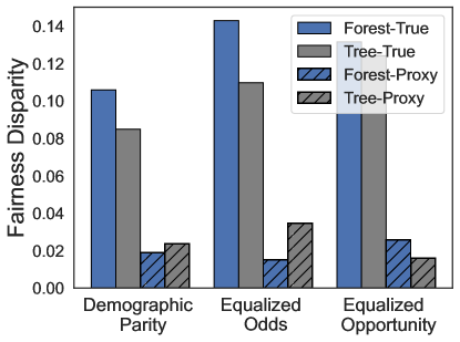
Figure 1: Fairness disparities of models on COMPAS (Angwin et al., 2016). True (or Proxy): Disparities using ground-truth sensitive attribute values (or proxy model’s predictions). Forest (or Tree): Random forest (or decisions tree) models. Observations: 1) Models considered as fair according to proxies can be actually unfair (True vs. Proxy), giving a false sense of fairness. 2) Fairness misperception (Forest vs. Tree) can cause practitioners to deploy wrong models.

Despite the popularity of this simple approach, few prior works have studied the efficacy or considered the practical constraints imposed by ethical concerns. In terms of efficacy, it remains unclear to what degrees we can trust a reported fairness measure based on proxies. A misleading fairness measure can trigger decline of trust and legal concerns. Unfortunately, this indeed happens frequently in practice. For example, Figure 1 shows the estimated fairness vs. true fairness on COMPAS (Angwin et al., 2016) dataset with race as the sensitive attribute. We use proxy models to predict race from last name. There are two observations: 1) Models considered as fair according to proxies are actually unfair. The Proxy fairness disparities ($0.02$) can be much smaller than the True fairness disparities ($>0.10$), giving a false sense of fairness. 2) Fairness misperception can be misleading in model selection. The proxy disparities mistakenly indicate random forest models have smaller disparities (DP and EOd) than decision tree models, but in fact it is the opposite.

In terms of ethical concerns, there is a growing worry on using proxies to infer sensitive information without user consent (Twitter, 2021; Fosch-Villaronga et al., 2021; Leslie, 2019; Kilbertus et al., 2017). Not unreasonably argued, using highly accurate proxies would reveal user’s private information. We argue that practitioners should use inaccurate or weak proxies whose noisy predictions would add additional protection to user privacy. However, if we merely compute fairness in the traditional way, the inaccuracy would propagate from weak proxies to the measured fairness metrics. To this end, we desire an algorithm that uses weak proxies only but can still accurately measure fairness.

We ask three questions: (1) Is directly using proxies efficacious in measuring fairness? (2) If not, is it possible to accurately evaluate fairness using proxies only? (3) Given the ethical controversy over inferring user private information, is it possible to only use weak proxies to protect privacy?

We address those questions as follows:

• Directly using proxies can be misleading: We theoretically show that directly using proxy models to estimate fairness would lead to a fairness metric whose estimation can be off by a quantity proportional to the prediction error of proxy models and the true fairness disparity (Theorem 3.2, Corollary 3.3).

• Provable algorithm using only weak proxies: We propose an algorithm (Figure 2, Algorithm 1) to calibrate the fairness metrics. We prove the error upper bound of our algorithm (Theorem 4.5, Corollary 4.7). We further show three weak proxy models with certain desired properties are sufficient and necessary to give unbiased fairness estimations using our algorithm (Theorem 4.6).

• Practical guidelines: We provide a set of practical guidelines to practitioners, including when to directly use the proxy models, when to use our algorithm to calibrate, how many proxy models are needed, and how to choose proxy models.

• Empirical studies: Experiments on COMPAS and CelebA consolidate our theoretical findings and show our calibrated fairness is significantly more accurately than baselines. We also show our algorithm can lead to better mitigation results.

The paper is organized as follows. Section 2 introduces necessary preliminaries. Section 3 analyzes what happens when we directly use proxies, and shows it can give misleading results, which motivates our algorithm. Section 4 introduces our algorithm that only uses weak proxies and instructions on how to use it optimally. Section 5 shows our experimental results. Section 6 discusses related works and Section 7 concludes the paper.

2 Preliminaries

Consider a $K$-class classification problem and a dataset $D{{{}^{\circ}}}:=\{(x_{n},y_{n})|n\in[N]\}$, where $N$ is the number of instances, $x_{n}$ is the feature, and $y_{n}$ is the label. Denote by $\mathcal{X}$ the feature space, $\mathcal{Y}=[K]:=\{1,2,\cdots,K\}$ the label space, and $(X,Y)$ the random variables of $(x_{n},y_{n}),\forall n$. The target model $f:\mathcal{X}\rightarrow[K]$ maps $X$ to a predicted label class $f(X)\in[K]$. We aim at measuring group fairness conditioned on a sensitive attribute $A\in[M]:=\{1,2,\cdots,M\}$ which is unavailable in $D{{{}^{\circ}}}$. Denote the dataset with ground-truth sensitive attributes by $D:=\{(x_{n},y_{n},a_{n})|n\in[N]\}$, the joint distribution of $(X,Y,A)$ by $\mathcal{D}$. The task is to estimate the fairness metrics of $f$ on $D{{}^{\circ}}$ without sensitive attributes such that the resulting metrics are as close to the fairness metrics evaluated on $D$ (with true $A$) as possible. We provide a summary of notations in Appendix A.1.

We consider three group fairness definitions and their corresponding measurable metrics: demographic parity (DP) (Calders et al., 2009; Chouldechova, 2017), equalized odds (EOd) (Woodworth et al., 2017), and equalized opportunity (EOp) (Hardt et al., 2016). All our discussions in the main paper are specific to DP defined as follows but we include the complete derivations for EOd and EOp in Appendix.

Definition 2.1 (Demographic Parity).

The demographic parity metric of $f$ on $\mathcal{D}$ conditioned on $A$ is defined as:

$$\Delta^{\textsf{DP}}(\mathcal{D},f):=\frac{1}{M(M-1)K}\cdot\sum_{\begin{subarray}{c}a,a^{\prime}\in[M]\\ k\in[K]\end{subarray}}|\mathbb{P}(f(X)=k|A=a)-\mathbb{P}(f(X)=k|A=a^{\prime})|.$$

Matrix-form Metrics.    For later derivations, we define matrix ${\bm{H}}$ as an intermediate variable. Each column of ${\bm{H}}$ denotes the probability needed for evaluating fairness with respect to $f(X)$. For DP, ${\bm{H}}$ is a $M\times K$ matrix with $H{[a,k]}:=\mathbb{P}(f(X)=k|A=a).$ The $a$-th row, $k$-th column, and $(a,k)$-th element of ${\bm{H}}$ are denoted by ${\bm{H}}[a],{\bm{H}}[:,k]$, and ${\bm{H}}[a,k]$, respectively. Then $\Delta^{\textsf{DP}}(\mathcal{D},f)$ in Definition 2.1 can be rewritten as:

Definition 2.2 (DP - Matrix Form).

$$\Delta^{\textsf{DP}}(\mathcal{D},f):=\frac{1}{M(M-1)K}\sum_{\begin{subarray}{c}a,a^{\prime}\in[M]\\ k\in[K]\end{subarray}}|{\bm{H}}[a,k]-{\bm{H}}[a^{\prime},k]|.$$

See definitions for EOd and EOp in Appendix A.2.

Proxy Models.    The conventional way to measure fairness is to approximate $A$ with an proxy model $g:\mathcal{X}\rightarrow[M]$ (Ghazimatin et al., 2022; Awasthi et al., 2021; Chen et al., 2019) and get proxy (noisy) sensitive attribute $\widetilde{A}:=g(X)$.

Transition Matrix.    The relationship between ${\bm{H}}$ and $\widetilde{\bm{H}}$ is largely dependent on the relationship between $A$ and $\widetilde{A}$ because it is the only variable that differs. Define matrix ${\bm{T}}$ to be the transition probability from $A$ to $\widetilde{A}$ where $(a,\tilde{a})$-th element is $T[a,\tilde{a}]=\mathbb{P}(\widetilde{A}=\tilde{a}|A=a)$. Similarly, denote by ${\bm{T}}_{k}$ the local transition matrix conditioned on $f(X)=k$, where the $(a,\tilde{a})$-th element is $T_{k}[{a,\tilde{a}}]:=\mathbb{P}(\widetilde{A}=\tilde{a}|f(X)=k,A=a)$. We further define clean (i.e. ground-truth) prior probability of $A$ as ${\bm{p}}:=[\mathbb{P}(A=1),\cdots,\mathbb{P}(A=M)]^{\top}$ and the noisy (predicted by proxies) prior probability of $\widetilde{A}$ as $\tilde{\bm{p}}:=[\mathbb{P}(\widetilde{A}=1),\cdots,\mathbb{P}(\widetilde{A}=M)]^{\top}$.

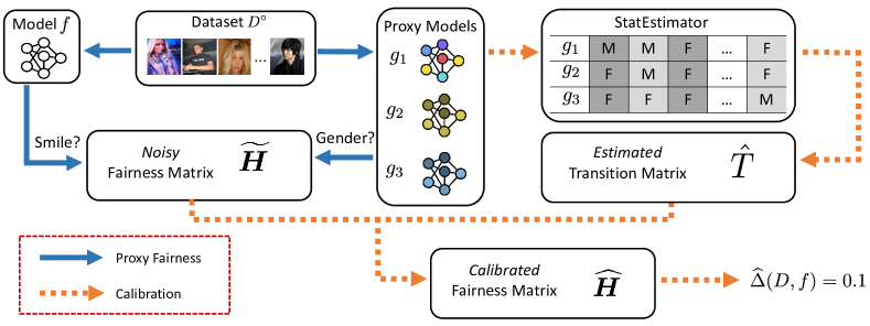
Figure 2: Overview of our algorithm that estimates fairness using only weak proxy models. We first directly estimate the noisy fairness matrix with proxy models (blue arrows), and then calibrate the estimated fairness matrix (orange arrows).

3 Proxy Results Can be Misleading

This section provides an analysis on how much the measured fairness-if using proxies naively-can deviate from the reality.

Using Proxy Models Directly.    Consider a scenario with $C$ proxy models denoted by the set $\mathcal{G}:=\{g_{1},\cdots,g_{C}\}$. The noisy sensitive attributes are denoted as $\widetilde{A}_{c}:=g_{c}(X),\forall c\in[C]$ and the corresponding target dataset with $\widetilde{A}$ is $\widetilde{D}:=\{(x_{n},y_{n},(\tilde{a}_{n}^{1},\cdots,\tilde{a}_{n}^{C}))|n\in[N]\}$, drawn from a distribution $\widetilde{\mathcal{D}}$. Similarly, by replacing $A$ with $\widetilde{A}$ in ${\bm{H}}$, we can compute $\widetilde{\bm{H}}$, which is the matrix-form noisy fairness metric estimated by the proxy model $g$ (or $\mathcal{G}$ if multiple proxy models are used). Define the directly measured fairness metric of $f$ on $\widetilde{\mathcal{D}}$ as follows.

Definition 3.1 (Proxy Disparity - DP).

$$\Delta^{\textsf{DP}}(\widetilde{\mathcal{D}},f):=\frac{1}{M(M-1)K}\sum_{\begin{subarray}{c}a,a^{\prime}\in[M]\\ k\in[K]\end{subarray}}|\widetilde{\bm{H}}[a,k]-\widetilde{\bm{H}}[a^{\prime},k]|.$$

Estimation Error Analysis.    We study the error of proxy disparity and give practical guidelines implied by analysis.

Intuitively, the estimation error of proxy disparity depends on the error of the proxy model $g$. Recall ${\bm{p}}$, $\tilde{\bm{p}}$, ${\bm{T}}$ and ${\bm{T}}_{k}$ are clean prior, noisy prior, global transition matrix, and local transition matrix. Denote by $\bm{{\bm{\Lambda}}}_{\tilde{\bm{p}}}$ and $\bm{{\bm{\Lambda}}}_{{\bm{p}}}$ the square diagonal matrices constructed from $\tilde{\bm{p}}$ and ${\bm{p}}$. We formally prove the upper bound of estimation error for the directly measured metrics in Theorem 3.2 (See Appendix B.1 for the proof).

Theorem 3.2 (Error Upper Bound of Proxy Disparities).

Denote by $\textsf{Err}^{\textsf{raw}}:=|\widetilde{\Delta}^{\textsf{DP}}(\widetilde{\mathcal{D}},f)-\Delta^{\textsf{DP}}(\mathcal{D},f)|$ the estimation error of the proxy disparity. Its upper bound is:

where $\bar{h}_{k}:=\frac{1}{M}\sum\limits_{a\in[M]}H[a,k]$, $\delta_{k}:=\max\limits_{a\in[M]}~{}|H[a,k]-\bar{h}_{k}|$.

It shows the error of proxy disparity depends on:

• $\bar{h}_{k}$: The average confidence of $f(X)$ on class $k$ over all sensitive groups. For example, if $f$ is a crime prediction model and $A$ is race, a biased $f$ (Angwin et al., 2016) may predict that the crime ($k=1$) rate for different races are 0.1, 0.2 and 0.6 respectively, then $\bar{h}_{1}=\frac{0.1+0.2+0.6}{3}=0.3$, and it is an approximation (unweighted by sample size) of the average crime rate over the entire population. The term depends on $\mathcal{D}$ and $f$ only (i.e. the true fairness disparity), and independent of any estimation algorithm.

• $\delta_{k}$: The maximum disparity between confidence of $f(X)$ on class $k$ and average confidence $\bar{h}_{k}$ across all sensitive groups. Using the same example, $\delta_{1}=\max(|0.1-0.3|,|0.2-0.3|,|0.6-0.3|)=0.3$. It is an approximation of the underlying fairness disparity, and larger $\delta_{k}$ indicates $f$ is more biased on $\mathcal{D}$. The term is also dependent on $\mathcal{D}$ and $f$ (i.e. the true fairness disparity), and independent of any estimation algorithm.

• Conditional Independence Violation: The term is dependent on the proxy model $g$’s prediction $\tilde{A}$ in terms of the transition matrix (${\bm{T}}$ and ${\bm{T}}_{k}$) and noisy prior probability ($\tilde{\bm{p}}$). The term goes to $0$ when ${\bm{T}}={\bm{T}}_{k}$, which implies $\tilde{A}$ and $f(X)$ are independent conditioned on $A$. This is the common assumption made in the prior work (Awasthi et al., 2021; Prost et al., 2021; Fogliato et al., 2020). And this term measures how much the conditional independence assumption is violated.

• Error of $g$: The term depends on the proxy model $g$. It goes to $0$ when ${\bm{T}}_{k}={\bm{I}}$ which implies the error rates of $g$’s prediction is $0$, i.e. $g$ is perfectly accurate. It measures the impact of $g$’s error on the fairness estimation error.

Case Study.    To help better understand the upper bound, we consider a simplified case when both $f$ and $A$ are binary. We further assume the conditional independence condition to remove the third term listed above in Theorem 3.2. See Appendix A.3 for the formal definition of conditional independence. Corollary 3.3 summarizes the result.

Corollary 3.3.

For a binary classifier $f$ and a binary sensitive attribute $A\in\{1,2\}$, when ($\tilde{A}\mathchoice{\mathrel{\hbox to0.0pt{$\displaystyle\perp$\hss}\mkern 2.0mu{\displaystyle\perp}}}{\mathrel{\hbox to0.0pt{$\textstyle\perp$\hss}\mkern 2.0mu{\textstyle\perp}}}{\mathrel{\hbox to0.0pt{$\scriptstyle\perp$\hss}\mkern 2.0mu{\scriptstyle\perp}}}{\mathrel{\hbox to0.0pt{$\scriptscriptstyle\perp$\hss}\mkern 2.0mu{\scriptscriptstyle\perp}}}f(X)|A$) holds, Theorem 3.2 is simplified to

where $\delta=|\mathbb{P}(f(X)=1|A=1)-\mathbb{P}(f(X)=1|A=2)|$.

Corollary 3.3 shows the estimation error of proxy disparity is proportional to the true underlying disparity between sensitive groups (i.e. $\delta$) and the proxy model’s error rates. In other words, the uncalibrated metrics can be highly inaccurate when $f$ is highly biased or $g$ has poor performance. This leads to the following suggestions:

Guidelines for Practitioners.    We should only trust the estimated fairness from proxy models when (1) the proxy model $g$ has good performance and (2) the true disparity is small (i.e. the target model $f$ is not highly biased).

In practice, both conditions required to trust the proxy results are frequently violated. When we want to measure $f$’s fairness, often we already have some fairness concerns and therefore the underlying fairness disparity is unlikely to be negligible. And the proxy model $g$ is usually inaccurate due to privacy concerns (discussed in Section 4.2) and distribution shift. This motivates us to develop an approach for more accurate estimates.

4 Weak Proxies Suffice

In this section, we show that by properly using a set of proxy models, we are able to guarantee an unbiased estimate of the true fairness measures.

4.1 Proposed Algorithm

With a given proxy model $g$ that labels sensitive attributes, we can anatomize the relationship between the true disparity and the proxy disparity. The following theorem targets DP  and see Appendix B.2 for results with respect to EOd and EOp and their proofs.

Theorem 4.1.

[Closed-form Relationship (DP)] The closed-form relationship between the true fairness vector ${\bm{H}}[:,k]$ and the noisy fairness vector $\widetilde{\bm{H}}[:,k]$ is the following:

Insights.    Theorem 4.1 reveals that the proxy disparity and the corresponding true disparity are related in terms of three key statistics: noisy prior $\tilde{\bm{p}}$, clean prior ${\bm{p}}$, and local transition matrix ${\bm{T}}_{k}$. Ideally, if we have the ground-truth values of them, we can calibrate the noisy fairness vectors to their corresponding ground-truth vectors (and therefore obtaining the perfectly accurate fairness metrics) usingTheorem 4.1. Hence, the most important step is to estimate ${\bm{T}}_{k}$, ${\bm{p}}$, and $\tilde{\bm{p}}$ without knowing the ground-truth values of $A$. Once we have those estimated key statistics, we can easily plug them into the above equation as the calibration step. Figure 2 shows the overview of our algorithm.

Algorithm 1 Fairness calibration algorithm (DP)

1:  Input: A set of proxy models $\mathcal{G}=\{g_{1},\cdots,g_{C}\}$. Target dataset $D{{}^{\circ}}$. Target model $f$. Transition matrix and prior probability estimator StatEstimator. # Predict sensitive attributes using all $g\in\mathcal{G}$

2:  $\tilde{a}_{n}^{c}\leftarrow g_{c}(x_{n}),\forall c\in[C],n\in[N]$ # Build the dataset with noisy sensitive attributes

3:  $\widetilde{D}\leftarrow\{(x_{n},y_{n},(\tilde{a}_{n}^{1},\cdots,\tilde{a}_{n}^{C}))|n\in[N]\}$ # Estimate fairness matrix and prior with sample mean

4:  $\widetilde{\bm{H}},\tilde{\bm{p}}\leftarrow\texttt{DirectEst}(\widetilde{D},f)$ # Estimate key statistics: ${\bm{p}}$ and ${\bm{T}}_{k}$

5:  $\{\widehat{\bm{T}}_{1},\cdots,\widehat{\bm{T}}_{K}\},\hat{\bm{p}}\leftarrow\texttt{StatEstimator}(\widetilde{D},f)$ # Calibrate each fairness vector with Theorem 4.1

6:  $\forall k\in[K]:\widehat{\bm{H}}[:,k]\leftarrow(\widehat{\bm{T}}_{k}^{\top}{\bm{\Lambda}}_{\hat{\bm{p}}})^{-1}{\bm{\Lambda}}_{\tilde{{\bm{p}}}}\widetilde{\bm{H}}[:,k]$ # Calculate the final fairness metric as Definition 2.2

7:  $\widehat{\Delta}(\widetilde{D},f)\leftarrow\frac{1}{M(M-1)K}\sum_{\begin{subarray}{c}a,a^{\prime}\in[M]\\ k\in[K]\end{subarray}}|\widehat{\bm{H}}[a,k]-\widehat{\bm{H}}[a^{\prime},k]|.$

8:  Output: The calibrated fairness metric $\widehat{\Delta}(\widetilde{D},f)$

Algorithm.    We summarize the method in Algorithm 1. In Line 4, we use sample mean in the uncalibrated form to estimate $\widetilde{\bm{H}}$ as $\widetilde{H}[\tilde{a},k]=\mathbb{P}(f(X)=k|\widetilde{A}=\tilde{a})\approx\frac{1}{N}\sum_{n=1}^{N}\mathds{1}(f(x_{n}=k|\tilde{a}_{n}=\tilde{a}))$ and $\tilde{\bm{p}}$ as $\tilde{\bm{p}}[\tilde{a}]=\mathbb{P}(\widetilde{A}=\tilde{a})\approx\frac{1}{N}\sum_{n=1}^{N}\mathds{1}(\tilde{a}_{n}=\tilde{a})$, $\forall\tilde{a}\in[M]$. In Line 5, we plug in an existing transition matrix and prior probability estimator to estimate ${\bm{T}}_{k}$ and ${\bm{p}}$ with only mild adaption that will be introduced shortly. Note that although we choose a specific estimator, our algorithm is a flexible framework that is compatible with any StatEstimator proposed in the noisy label literature (Liu and Chen, 2017; Zhu et al., 2021b, 2022).

Details: Estimating Key Statistics.    The algorithm requires us to estimate ${\bm{T}}_{k}$ and ${\bm{p}}$ based on the predicted $\widetilde{A}$ by proxy models. In the literature of noisy learning, there exists several feasible algorithms (Liu and Tao, 2015; Scott, 2015; Patrini et al., 2017; Northcutt et al., 2021; Zhu et al., 2021b). We choose HOC (Zhu et al., 2021b) because it has stronger theoretical guarantee and lower sample complexity than most existing estimators. Intuitively, if given three proxy models, the joint distributions of their predictions would encode ${\bm{T}}_{k}$ and ${\bm{p}}$, i.e. $\mathbb{P}(\widetilde{A}_{1},\widetilde{A}_{2},\widetilde{A}_{3})=\textsf{Func}(\{{\bm{T}}_{k}\}_{k\in[K]},{\bm{p}})$. For example, with Chain rule and independence among proxy predictions conditioned on $A$, we have:

$$\mathbb{P}(\widetilde{A}_{1}=\tilde{a}_{1},\widetilde{A}_{2}=\tilde{a}_{2},\widetilde{A}_{3}=\tilde{a}_{3}|f(X)=k)=\sum_{a\in[M]}\mathbb{P}(A=a|f(X)=k)\cdot T_{k}[a,\tilde{a}_{1}]\cdot T_{k}[a,\tilde{a}_{2}]\cdot T_{k}[a,\tilde{a}_{3}].$$

HOC counts the frequency of different $(\widetilde{A}_{1},\widetilde{A}_{2},\widetilde{A}_{3})$ patterns to obtain LHS and solve equations to get $T_{k}$’s in the RHS. See more details of our implementations in Appendix C.1–C.2 and HOC in Appendix C.3.

4.2 Requirements of Proxy Models

To use our algorithm, there are two practical questions for practitioners: 1) what properties proxy models should satisfy and 2) how many proxy models are needed. The first question is answered by two requirements made in the estimation algorithm HOC:

Requirement 4.2 (Informativeness of Proxies).

The noisy attributes given by each proxy model $g$ are informative, i.e. $\forall k\in[M]$, 1) ${\bm{T}}_{k}$ is non-singular and 2) either $T_{k}[a,a]>\mathbb{P}(\widetilde{A}=a|f(X)=k)$ or $T_{k}[a,a]>T_{k}[a,a^{\prime}],\forall a^{\prime}\neq a$.

Requirement 4.2 is the prerequisite of getting a feasible and unique estimate of ${\bm{T}}_{k}$ (Zhu et al., 2021b), where the non-singular requirement ensures the matrix inverse in Theorem 4.1 exists and the constraints on $T_{k}[a,a]$ describes the worst tolerable performance of $g$. When $M=2$, the constraints can be simplified as $T_{k}[1,2]+T_{k}[2,1]<1$ (Liu and Chen, 2017; Liu and Guo, 2020), i.e. $g$’s predictions are better than random guess in binary classification. If this requirement is violated, there might exist more than one feasible estimates of ${\bm{T}}_{k}$, making the problem insoluble.

The above requirement is weak. The proxies are merely required to positively correlate with the true sensitive attributes. We discuss the privacy implication of using weak proxies shortly after.

Requirement 4.3 (Independence between Proxies).

The noisy attributes predicted by proxy models $g_{1}(X),\cdots,g_{C}(X)$ are independent and identically distributed (i.i.d.) given $A$.

Requirement 4.3 ensures the additional two proxy models provide more information than using only one classifier. If it is violated, we would still get an estimate but may be inaccurate. Note this requirement is different from the conditional independence often assumed in the fairness literature (Awasthi et al., 2021; Prost et al., 2021; Fogliato et al., 2020), which is $g(X)\mathchoice{\mathrel{\hbox to0.0pt{$\displaystyle\perp$\hss}\mkern 2.0mu{\displaystyle\perp}}}{\mathrel{\hbox to0.0pt{$\textstyle\perp$\hss}\mkern 2.0mu{\textstyle\perp}}}{\mathrel{\hbox to0.0pt{$\scriptstyle\perp$\hss}\mkern 2.0mu{\scriptstyle\perp}}}{\mathrel{\hbox to0.0pt{$\scriptscriptstyle\perp$\hss}\mkern 2.0mu{\scriptscriptstyle\perp}}}f(X)|A$ rather than ours $g_{1}(X)\mathchoice{\mathrel{\hbox to0.0pt{$\displaystyle\perp$\hss}\mkern 2.0mu{\displaystyle\perp}}}{\mathrel{\hbox to0.0pt{$\textstyle\perp$\hss}\mkern 2.0mu{\textstyle\perp}}}{\mathrel{\hbox to0.0pt{$\scriptstyle\perp$\hss}\mkern 2.0mu{\scriptstyle\perp}}}{\mathrel{\hbox to0.0pt{$\scriptscriptstyle\perp$\hss}\mkern 2.0mu{\scriptscriptstyle\perp}}}g_{2}(X)\mathchoice{\mathrel{\hbox to0.0pt{$\displaystyle\perp$\hss}\mkern 2.0mu{\displaystyle\perp}}}{\mathrel{\hbox to0.0pt{$\textstyle\perp$\hss}\mkern 2.0mu{\textstyle\perp}}}{\mathrel{\hbox to0.0pt{$\scriptstyle\perp$\hss}\mkern 2.0mu{\scriptstyle\perp}}}{\mathrel{\hbox to0.0pt{$\scriptscriptstyle\perp$\hss}\mkern 2.0mu{\scriptscriptstyle\perp}}}g_{3}(X)|A$.

The second question (how many proxy models are needed) has been answered by Theorem 5 in Liu (2022), which we summarize in the following.

Lemma 4.4.

If satisfying Requirements 4.2–4.3, three proxy models are both sufficient and necessary to identify ${\bm{T}}_{k}$.

How to Protect Privacy with Weak Proxies.    Intuitively, weak proxies can protect privacy better than strong proxies due to their noisier predictions. We connect weak proxy’s privacy-preserveness to differential privacy (Ghazi et al., 2021). Assume misclassification probability on $\widetilde{A}$ is bounded across all samples, i.e.

$$\max_{x\in X}{\mathbb{P}(\widetilde{A}=a|A=a,X=x)}\leq 1-\epsilon_{0}$$

and

$$\min_{x\in X}{\mathbb{P}(\widetilde{A}=a|A=a^{\prime},X=x)}\geq\epsilon_{1}$$

for $a\in[M],a^{\prime}\in[M],a\neq a^{\prime}$. Then the proxy predictions satisfy $\ln(\frac{1-\epsilon_{0}}{\epsilon_{1}})$-DP. See Appendix B.6 for the proof.

In practice, if the above assumption does not hold naturally by proxies, we can add noise to impose it. When practitioners think proxies are too strong, they can add additional noise to reduce informativeness, further protecting privacy. Later we will show in Table 2 that our algorithm is robust in estimation accuracy when adding noise to proxy predictions. When we intentionally make the proxies weaker by flipping predicted sensitive attributes with probability $0.4$, resulting in only $58.45\%$ proxy accuracy, it corresponds to $0.41$-DP ($\epsilon_{0}=\epsilon_{1}=0.4$) protection.

4.3 Theoretical Guarantee

We theoretically analyze estimation error on our calibrated metrics in a similar way as in Section 3. Denote by $\widehat{\Delta}^{\textsf{DP}}(\widetilde{\mathcal{D}},f)$ the calibrated DP disparity evaluated on our calibrated fairness matrix $\widehat{\bm{H}}$. We have:

Theorem 4.5 (Error Upper Bound of Calibrated Metrics).

Denote the estimation error of the calibrated fairness metrics by $\textsf{Err}^{\textsf{cal}}:=|\widehat{\Delta}^{\textsf{DP}}(\widetilde{\mathcal{D}},f)-\Delta^{\textsf{DP}}(\mathcal{D},f)|$. Then:

where $\varepsilon(\widehat{\bm{T}}_{k},\hat{\bm{p}}):=\|{\bm{\Lambda}}_{{\hat{\bm{p}}}}^{-1}{\bm{\Lambda}}_{{{\bm{p}}}}-{\bm{I}}\|_{1}\|{\bm{T}}_{k}\widehat{\bm{T}}_{k}^{-1}\|_{1}+\|{\bm{I}}-{\bm{T}}_{k}\widehat{\bm{T}}_{k}^{-1}\|_{1}$ is the error induced by calibration. With a perfect estimator $\widehat{\bm{T}}_{k}={\bm{T}}_{k}$ and $\hat{\bm{p}}_{k}={\bm{p}}_{k},\forall k\in[K]$, we have $\textsf{Err}^{\textsf{cal}}=0$.

Theorem 4.5 shows the upper bound of estimation error mainly depends on the estimates $\widehat{\bm{T}}_{k}$ and $\hat{\bm{p}}$, i.e. the following two terms in $\varepsilon(\widehat{\bm{T}}_{k},\hat{\bm{p}})$: $\|{\bm{\Lambda}}_{{\hat{\bm{p}}}}^{-1}{\bm{\Lambda}}_{{{\bm{p}}}}-{\bm{I}}\|_{1}\|{\bm{T}}_{k}\widehat{\bm{T}}_{k}^{-1}\|_{1}$ and $\|{\bm{I}}-{\bm{T}}_{k}\widehat{\bm{T}}_{k}^{-1}\|_{1}$. When the estimates are perfect, i.e. $\widehat{\bm{T}}_{k}={\bm{T}}_{k}$ and $\hat{\bm{p}}={\bm{p}}$, then both terms go to 0 because ${\bm{\Lambda}}_{{\hat{\bm{p}}}}^{-1}{\bm{\Lambda}}_{{{\bm{p}}}}={\bm{I}}$ and ${\bm{T}}_{k}\widehat{\bm{T}}_{k}^{-1}={\bm{I}}$. Together with Lemma 4.4, we can show the optimality of our algorithm as follows.

Theorem 4.6.

When Requirements 4.2–4.3 hold for three proxy models, the calibrated fairness metrics given by Algorithm 1 with key statistics estimated by Algorithm 2 achieve zero error, i.e. $|\widehat{\Delta}^{\textsf{DP}}(\widetilde{\mathcal{D}},f)-\Delta^{\textsf{DP}}(\mathcal{D},f)|=0$.

Besides, we compare the error upper bound of our method with the exact error (not its upper bond) in the case of Corollary 3.3, and summarize the result in Corollary 4.7.

Corollary 4.7.

For a binary classifier $f$ and a binary sensitive attribute $A\in\{1,2\}$, when ($\tilde{A}\mathchoice{\mathrel{\hbox to0.0pt{$\displaystyle\perp$\hss}\mkern 2.0mu{\displaystyle\perp}}}{\mathrel{\hbox to0.0pt{$\textstyle\perp$\hss}\mkern 2.0mu{\textstyle\perp}}}{\mathrel{\hbox to0.0pt{$\scriptstyle\perp$\hss}\mkern 2.0mu{\scriptstyle\perp}}}{\mathrel{\hbox to0.0pt{$\scriptscriptstyle\perp$\hss}\mkern 2.0mu{\scriptscriptstyle\perp}}}f(X)|A$) and ${\bm{p}}=[0.5,0.5]^{\top}$, the proposed calibration method is guaranteed to be more accurate than the uncalibrated measurement, i.e. , $\textsf{Err}^{\textsf{cal}}\leq\textsf{Err}^{\textsf{raw}}$, if

Corollary 4.7 shows when the error $\varepsilon(\widehat{\bm{T}}_{k},\hat{\bm{p}})$ that is induced by inaccurate $\widehat{\bm{T}}_{k}$ and $\hat{\bm{p}}$ is below the threshold $\gamma$, our method is guaranteed to lead to a smaller estimation error compared to the uncalibrated measurement under the considered setting. The threshold implies that, adopting our method rather than the uncalibrated measurement can be greatly beneficial when $e_{1}$ and $e_{2}$ are high (i.e. $g$ is inaccurate) or when the normalized (true) fairness disparity $\frac{\Delta^{\textsf{DP}}(\mathcal{D},f)}{\|{\bm{H}}[:,k^{\prime}]\|_{1}}$ is high (i.e. $f$ is highly biased).

4.4 Guidelines for Practitioners

We provide a set of guidelines implied by our theoretical results.

When to Use Our Algorithm.    Corollary 4.7 shows that our algorithm is preferred over directly using proxies when 1) the proxy model $g$ is weak or 2) the true disparity is large.

How to Best Use Our Algorithm.    Section 4.2 implies a set of principles for selecting proxy models:

• [Requirement 4.2] Even if proxy models are weak, as long as they are informative, e.g. in binary case the performance is better than random guess, then it is enough for estimations.

• [Requirement 4.3] We should try to make sure the predictions of proxy models are i.i.d., which is more important than using more proxy models. One way of doing it is to choose proxy models trained on different data sources.

• [Lemma 4.4] At least three proxy models are prefered.

Table 1: Normalized estimation error on COMPAS. True disparity: $\sim 0.2$. Average accuracy of weak proxy models: 68.85%.

COMPAS	DP Normalized Error (%) $\downarrow$				EOd Normalized Error (%) $\downarrow$				EOp Normalized Error (%) $\downarrow$
Target models $f$	Base	Soft	Global	Local	Base	Soft	Global	Local	Base	Soft	Global	Local
tree	43.82	61.26	22.29	39.81	45.86	63.96	23.09	42.81	54.36	70.15	13.27	49.49
forest	43.68	60.30	19.65	44.14	45.60	62.85	18.56	44.04	53.83	69.39	17.51	63.62
boosting	43.82	61.26	22.29	44.64	45.86	63.96	23.25	49.08	54.36	70.15	13.11	54.67
SVM	50.61	66.50	30.95	42.00	53.72	69.69	32.46	47.39	59.70	71.12	29.29	51.31
logit	41.54	60.78	16.98	35.69	43.26	63.15	21.42	31.91	50.86	65.04	14.90	26.27
nn	41.69	60.55	19.48	34.22	43.34	62.99	19.30	43.24	54.50	68.50	14.20	59.95
compas_score	41.28	58.34	11.24	14.66	42.43	59.79	11.80	18.65	48.78	62.24	5.78	23.80

Table 2: Normalized error on CelebA. We simulate weak proxies by adding noise to predicted attributes according to Requirement 4.3 to bring down the performance of proxy models. Each row represents the noise magnitude and accuracy of proxy models, e.g. “$[0.2,0.0]$ (82.44%)” means $T[1,2]=0.2$, $T[2,1]=0.0$ and accuracy is 82.44%.

CelebA	DP Normalized Error (%) $\downarrow$				EOd Normalized Error (%) $\downarrow$				EOp Normalized Error (%) $\downarrow$
FaceNet512	Base	Soft	Global	Local	Base	Soft	Global	Local	Base	Soft	Global	Local
$[0.2,0.0]$ (82.44%)	7.37	11.65	20.58	5.05	25.06	26.99	6.43	0.10	24.69	27.27	11.11	1.07
$[0.2,0.2]$ (75.54%)	30.21	31.57	24.25	13.10	44.73	46.36	11.26	9.04	37.67	38.77	20.94	27.98
$[0.4,0.2]$ (65.36%)	51.32	54.56	19.42	10.47	62.90	65.10	11.09	19.15	56.51	58.73	23.86	23.55
$[0.4,0.4]$ (58.45%)	77.76	78.39	9.41	19.80	79.31	80.10	24.49	8.02	78.35	79.62	10.61	5.71

5 Experiments

5.1 Setup

We test the performance of our method on two real-world datasets: COMPAS (Angwin et al., 2016) and CelabA (Liu et al., 2015). We report results on all three group fairness metrics (DP, EOd, and EOp) whose true disparities (estimated using the ground-truth sensitive attributes) are denoted by $\Delta^{\textsf{DP}}(\mathcal{D},f)$, $\Delta^{\textsf{EOd}}(\mathcal{D},f)$, $\Delta^{\textsf{EOp}}(\mathcal{D},f)$ respectively. We train the target model $f$ on the dataset without using $A$, and use the proxy models downloaded from open-source projects. The detailed settings are the following:

• COMPAS (Angwin et al., 2016): Recidivism prediction data. Feature $X$: tabular data. Label $Y$: recidivism within two years (binary). Sensitive attribute $A$: race (black and non-black).Target models $f$ (trained by us): decision tree, random forest, boosting, SVM, logit model, and neural network (accuracy range 66%–70% for all models). Three proxy models ($g_{1},g_{2},g_{3}$): racial classifiers given name as input (Sood and Laohaprapanon, 2018) (average accuracy 68.85%).

• CelabA (Liu et al., 2015): Face dataset. Feature $X$: facial images. Label $Y$: smile or not (binary). Sensitive attribute $A$: gender (male and female). Target models $f$: ResNet18 (He et al., 2016) (accuracy 90.75%, trained by us). We use one proxy model ($g_{1}$): gender classifier that takes facial images as input (Serengil and Ozpinar, 2021), and then use the clusterability to simulate the other two proxy models (as Line 4 in Algorithm 2, Appendix C.1). Since the proxy model $g_{1}$ is highly accurate (accuracy 92.55%), which does not give enough privacy protection, we add noise to $g_{1}$’s predicted sensitive attributes according to Requirement 4.3. We generate the other two proxies ($g_{2}$ and $g_{2}$) based on $g_{1}$’s noisy predictions.

Method.

We propose a simple heuristic in our algorithm to stabilize estimation error on $\widehat{{\bm{T}}}_{k}$. Specifically, we use a single transition matrix $\widehat{{\bm{T}}}$ estimated once on the full dataset $\widetilde{D}$ as Line 8 of Algorithm 2 (Appendix C.1) to approximate ${{\bm{T}}}_{k}$. We name this heuristic as Global (i.e. ${\bm{T}}_{k}\approx\widehat{{\bm{T}}}$) and the original method (estimated on each data subset $\widetilde{D}_{k}:=\{(X,Y,A)|f(X)=k\}$, i.e. ${\bm{T}}_{k}\approx\widehat{{\bm{T}}}_{k}$) as Local. See Appendix D.4 for details. We compare with two baselines: the directly estimated metric without any calibration (Base) and Soft (Chen et al., 2019) which also only uses proxy models to calibrate the measured fairness by re-weighting metric with the soft predicted probability from the proxy model.

Evaluation Metric.    Let $\Delta(D,f)$ be the ground-truth fairness metric. For a given estimated metric $E$, we define three estimation errors: $\textsf{Raw Error}(E):=|E-\Delta(D,f)|,$ $\textsf{Normalized Error}(E):=\frac{\textsf{Raw Error(E)}}{{\Delta(D,f)}},$ and $\textsf{Improvement}(E):=1-\frac{\textsf{Raw Error(E)}}{\textsf{Raw Error(Base)}},$ where Base is the directly measured metric.

5.2 Results and Analyses

COMPAS Results.    Table 1 reports the normalized error on COMPAS (See Table 7 in Appendix D.1 for the other two evaluation metrics). There are two main observations. First, our calibrated metrics outperform baselines with a big margin on all three fairness definitions. Compared to Base, our metrics are 39.6%–88.2% more accurate (Improvement). As pointed out by Corollary 4.7, this is because the target models $f$ are highly biased (Table 6) and the proxy models $g$ are inaccurate (accuracy 68.9%). As a result, Base has large normalized error (40–60%). Second, Global outperforms Local, since with inaccurate proxy models, Requirements 4.2–4.3 on HOC may not hold in local dataset, inducing large estimation errors in local estimates. Finally, we also include the results with three-class sensitive attributes (black, white, and others) in Appendix D.2.

CelebA Results.    Table 2 summarizes the key results (see Appendix D.3 for the full results). First, our algorithm outperform baselines significantly on all fairness definitions with all noise rates, which validates Corollary 4.7. When $g$ becomes less accurate, Base’s DP normalized error increases by more than $10$x while our error (Local) only increases by $3$x. Second, unlike COMPAS, Local now outperforms Global. This is because we add random noise following Requirement 4.3 and therefore the estimation error of Local is not increased significantly. This further consolidates our theoretical findings. Therefore when Requirement 4.3 is satisfied, using Local can give more accurate estimations than Global  (see Appendix D.4 for more discussions). In practice, practitioners can roughly examine Requirement 4.3 by running statistical tests like Chi-squared tests on proxy predictions.

Mitigating Disparity.    We further discuss the disparity mitigation built on our method. The aim is to improve the classification accuracy while ensuring fairness constraints. Particularly, we choose DP and test on CelebA, where $\widehat{\Delta}^{\textsf{DP}}(\widetilde{D},f)=0$ is the constraint for our method and $\widetilde{\Delta}^{\textsf{DP}}(\widetilde{D},f)=0$ is the constraint for the baseline (Base). Recall $\widehat{\Delta}^{\textsf{DP}}(\widetilde{D},f)$ is obtained from Algorithm 1 (Line 8), and $\widetilde{D}:=\{(x_{n},y_{n},\tilde{a}_{n})|n\in[N]\}$. Table 3 shows our methods with popular pre-trained feature extractors (rows other than Base) can consistently achieve both a lower DP disparity and a higher accuracy on the test data. Besides, our method can achieve the performance which is close to the mitigation with ground-truth sensitive attributes. We defer more details to Appendix D.5.

Table 3: Results (averaged by the last 5 epochs) of disparity mitigation. Base: Direct mitigation using noisy sensitive attributes. Ground-Truth: Mitigation using ground-truth sensitive attributes. Facenet, Facenet 512, etc.: Pre-trained models to generate feature representations that we use to simulate the other two proxy models.

CelebA	$\Delta^{\textsf{DP}}(D^{\text{test}},f)$ $\downarrow$	Accuracy $\uparrow$
Base	0.0578	0.8422
Ground-Truth	0.0213	0.8650
Facenet	0.0453	0.8466
Facenet512	0.0273	0.8557
OpenFace	0.0153	0.8600
ArcFace	0.0435	0.8491
Dlib	0.0265	0.8522
SFace	0.0315	0.8568

Guidelines for Practitioners.    The above experimental results lead to the following suggestions:

• Our algorithm can give a clear advantage over baselines when the proxy model $g$ is weak (e.g. error $\geq 15\%$) or the target model $f$ is highly biased (e.g. fairness disparity $\geq 0.1$).

• When using our algorithm, we should prefer Local when Requirement 4.3 is satisfied, i.e. proxies make i.i.d predictions; and prefer Global otherwise. In practice, practitioners can use statistical tests like Chi-squared tests to roughly judge if proxy predictions are independent or not.

6 Related Work

Fairness with Imperfect Sensitive Attributes.    Existing methods mostly fall into two categories. First, some assume access to ground-truth sensitive attributes on a data subset or label them if unavailable, e.g. Youtube asks its creators to voluntarily provide their demographic information (Wojcicki, 2021). But it either requires labeling resource or depends on the volunteering willingness, and it suffers from sampling bias. Second, some works assume there exists proxy datasets that can be used to train proxy models, e.g. Meta (Alao et al., 2021) and others (Elliott et al., 2009; Awasthi et al., 2021; Diana et al., 2022). However, they often assume proxy datasets and the target dataset are i.i.d., and some form of conditional independence, which can be violated in practice. In addition, since proxy datasets also contain sensitive information (i.e. the sensitive labels), it might be difficult to obtain such training data from the open-source projects. The closest work to ours is (Chen et al., 2019), which also assumes only proxy models. It is only applicable to demographic disparity, and we compare it in the experiments. Note that compared to the prior works, our algorithm only requires realistic assumptions. Specifically we drop many commonly made assumptions in the literature, i.e. 1) access to labeling resource (Wojcicki, 2021), 2) access to proxy model’s training data (Awasthi et al., 2021; Diana et al., 2022), 3) data i.i.d (Awasthi et al., 2021), and 4) conditional independence (Awasthi et al., 2021; Prost et al., 2021; Fogliato et al., 2020).

Noisy Label Learning.    Label noise may come from various sources, e.g., human annotation error (Xiao et al., 2015; Wei et al., 2022; Agarwal et al., 2016) and model prediction error (Lee et al., 2013; Berthelot et al., 2019; Zhu et al., 2021a), which can be characterized by transition matrix on label (Liu, 2022; Bae et al., 2022; Yang et al., 2021). Applying the noise transition matrix to ensure fairness is emerging (Wang et al., 2021; Liu and Wang, 2021; Lamy et al., 2019). There exist two lines of works for estimating transition matrix. The first line relies on anchor points (samples belonging to a class with high certainty) or their approximations (Liu and Tao, 2015; Scott, 2015; Patrini et al., 2017; Xia et al., 2019; Northcutt et al., 2021). These works requires training a neural network on the $(X,\widetilde{A}:=g(X))$. The second line of work, which we leverage, is data-centric (Liu and Chen, 2017; Liu et al., 2020; Zhu et al., 2021b, 2022) and training-free. The main idea is to check the agreements among multiple noisy attributes as discussed in Appendix C.3.

7 Conclusions and Discussions

Although it is appealing to use proxies to estimate fairness when sensitive attributes are missing, its ethical implications are causing practitioners to be cautious about adopting this approach. However simply giving up this practical and powerful solution shuts down the chance of studying fairness on a large scale. In this paper, we have offered a middle-way solution, i.e. by using only weak proxies, we can protect data privacy while still being able to measure fairness. To this end, we design an algorithm that, though only based on weak proxies, can still provably achieve accurate fairness estimations. We show our algorithm can effectively measure and mitigate bias, and provide a set of guidelines for practitioners on how to use proxies properly. We hope our work can inspire more discussions on this topic since the inability to access sensitive attributes ethically is currently a major obstacle to studying and promoting fairness.

Ethics Statement

Our goal is to better study and promote fairness. Without a promising estimation method, given the increasingly stringent privacy regulations, it would be difficult for academia and industry to measure, detect, and mitigate bias in many real-world scenarios. However, we need to caution readers that, needless to say, no estimation algorithm is perfect. Theoretically, in our algorithm, if the transition matrix is perfectly estimated, then our method can measure fairness with 100% accuracy. However, if Requirements 4.2–4.3 required by our estimator in Algorithm 2 do not hold, our calibrated metrics might have a non-negligible error, and therefore could be misleading. In addition, the example we use to explain terms in Theorem 3.2 is based on conclusions from [Angwin et al., 2016]. We do not have any biased opinion on the crime rate across different racial groups. Furthermore, we are fully aware that many sensitive attributes are not binary, e.g. race and gender. We use the binary sensitive attributes in experiments because 1) existing works have shown that bias exists in COMPAS between race black and others and 2) the ground-truth gender attribute in CelebA is binary. We also have experiments with three categories of races (black, white, others) in Appendix D.2. We summarize races other than black and white as others since their sample size is too small. Finally, all the data and models we use are from open-source projects, and the bias measured on them do not reflect our opinions about those projects.

Appendix

The Appendix is organized as follows.

• Section A presents a summary of notations, more fairness definitions, and a clear statement of the assumption that is common in the literature. Note our algorithm does not rely on this assumption.

• Section B presents the full version of our theorems (for DP, EOd, EOp), corollaries, and the corresponding proofs.

• Section C shows how HOC works and analyzes why other learning-centric methods in the noisy label literature may not work in our setting.

• Section D presents more experimental results.

Appendix A More Definitions and Assumptions

A.1 Summary of Notations

Table 4: Summary of key notations

Notation	Explanation
$\mathcal{G}:=\{g_{1},\cdots,g_{C}\}$	$C$ proxy models for generating noisy sensitive attributes
$X,Y,A,$ and $\widetilde{A}:=g(X)$	Random variables of feature, label, ground-truth sensitive attribute, and noisy sensitive attributes
$x_{n},y_{n},a_{n}$	The $n$-th feature, label, and ground-truth sensitive attribute in a dataset
$N,K,M$	The number of instances, label classes, categories of sensitive attributes
$[N]:=\{1,\cdots,N\}$	A set counting from $1$ to $N$
$\mathcal{X}$, $f:\mathcal{X}\rightarrow[K]$	Space of $X$, target model
$D{{{}^{\circ}}}:=\{(x_{n},y_{n})|n\in[N]\}$	Target dataset
$D:=\{(x_{n},y_{n},a_{n})|n\in[N]\}$	$D{{}^{\circ}}$ with ground-truth sensitive attributes
$\widetilde{D}:=\{(x_{n},y_{n},(\tilde{a}_{n}^{1},\cdots,\tilde{a}_{n}^{C}))|n\in[N]\}$	$D{{}^{\circ}}$ with noisy sensitive attributes
$(X,Y,A)\sim\mathcal{D},(X,Y,\widetilde{A})\sim\widetilde{\mathcal{D}}$	Distribution of $D$ and $\widetilde{D}$
$u\in\{\textsf{DP},\textsf{EOd},\textsf{EOp}\}$	A unified notation of fairness definitions, e.g., EOd, EOp, EOd
$\Delta^{u}(\mathcal{D},f),\widetilde{\Delta}^{u}(\widetilde{\mathcal{D}},f),\widehat{\Delta}^{u}(\widetilde{\mathcal{D}},f)$	True, (direct) noisy, and calibrated group fairness metrics on data distributions
$\Delta^{u}(D,f),\widetilde{\Delta}^{u}(\widetilde{D},f),\widehat{\Delta}^{u}(\widetilde{D},f)$	True, (direct) noisy, and calibrated group fairness metrics on datasets
${\bm{H}},{\bm{H}}[a],{\bm{H}}[:,k],{\bm{H}}[a,k]$	Fairness matrix, its $a$-th row, $k$-th column, $(a,k)$-th element
$\widetilde{\bm{H}}$	Noisy fairness matrix with respect to $\widetilde{A}$
${\bm{T}}$, $T[a,a\tilde{]}:=\mathbb{P}(\widetilde{A}=\tilde{a}|A=a)$	Global noise transition matrix
${\bm{T}}_{k}$, $T_{k}[a,a\tilde{]}:=\mathbb{P}(\widetilde{A}=\tilde{a}|A=a,f(X)=k)$	Local noise transition matrix
${\bm{p}}:=[\mathbb{P}(A=1),\cdots,\mathbb{P}(A=M)]^{\top}$	Clean prior probability
$\tilde{\bm{p}}:=[\mathbb{P}(\widetilde{A}=1),\cdots,\mathbb{P}(\widetilde{A}=M)]^{\top}$	Clean prior probability

A.2 More Fairness Definitions

We present the full version of fairness definitions and the corresponding matrix form for DP, EOd, and EOp as follows.

Fairness Definitions.    We consider three group fairness [Wang et al., 2020, Cotter et al., 2019, Chen et al., 2022] definitions and their corresponding measurable metrics: demographic parity (DP) [Calders et al., 2009, Chouldechova, 2017], equalized odds (EOd) [Woodworth et al., 2017], and equalized opportunity (EOp) [Hardt et al., 2016].

Definition 2.1 (Demographic Parity). The demographic parity metric of $f$ on $\mathcal{D}$ conditioned on $A$ is defined as:

$$\Delta^{\textsf{DP}}(\mathcal{D},f):=\frac{1}{M(M-1)K}\cdot$$

$$\sum_{\begin{subarray}{c}a,a^{\prime}\in[M]\\ k\in[K]\end{subarray}}|\mathbb{P}(f(X)=k|A=a)-\mathbb{P}(f(X)=k|A=a^{\prime})|.$$

Definition A.1 (Equalized Odds).

The equalized odds metric of $f$ on $\mathcal{D}$ conditioned on $A$ is:

$$\Delta^{\textsf{EOd}}(\mathcal{D},f)=\frac{1}{M(M-1)K^{2}}\sum_{\begin{subarray}{c}a,a^{\prime}\in[M]\\ k\in[K],y\in[K]\end{subarray}}|\mathbb{P}(f(X)=k|Y=y,A=a)-\mathbb{P}(f(X)=k|Y=y,A=a^{\prime})|.$$

Definition A.2 (Equalized Opportunity).

The equalized opportunity metric of $f$ on $\mathcal{D}$ conditioned on $A$ is:

$$\Delta^{\textsf{EOp}}(\mathcal{D},f)=\frac{1}{M(M-1)}\sum_{a,a^{\prime}\in[M]}|\mathbb{P}(f(X)=1|Y=1,A=a)-\mathbb{P}(f(X)=1|Y=1,A=a^{\prime})|.$$

Matrix-form Metrics.    To unify three fairness metrics in a general form, we represent them with a matrix ${\bm{H}}$. Each column of ${\bm{H}}$ denotes the probability needed for evaluating fairness with respect to classifier prediction $f(X)$. For DP, ${\bm{H}}{[:,k]}$ denotes the following column vector:

$${\bm{H}}{[:,k]}:=[\mathbb{P}(f(X)=k|A=1),\cdots,\mathbb{P}(f(X)=k|A=M)]^{\top}.$$

Similarly for EOd and EOp, let ${k\otimes y}:=K(k-1)+y$ be the 1-d flattened index that represents the 2-d coordinate in $f(X)\times Y$, ${\bm{H}}{[:,{k\otimes y}]}$ is defined as the following column vector:

$${\bm{H}}{[:,{k\otimes y}]}:=[\mathbb{P}(f(X)=k|Y=y,A=1),\cdots,\mathbb{P}(f(X)=k|Y=y,A=M)]^{\top}.$$

The sizes of ${\bm{H}}$ for DP, EOd  and EOp are $M\times K$, $M\times K^{2}$, and $M\times 1$ respectively. The noise transition matrix related to EOd and EOp is ${\bm{T}}_{k\otimes y}$, where the $(a,\tilde{a})$-th element is denoted by $T_{k\otimes y}[{a,\tilde{a}}]:=\mathbb{P}(\widetilde{A}=\tilde{a}|f(X)=k,Y=y,A=a)$.

A.3 Common Conditional Independence Assumption in the Literature

We present below a common conditional independence assumption in the literature [Awasthi et al., 2021, Prost et al., 2021, Fogliato et al., 2020]. Note our algorithm successfully drops this assumption.

Assumption A.3 (Conditional Independence).

$\tilde{A}$ and $f(X)$ are conditionally independent given $A$ (and $Y$ for EOd, EOp):

$$\text{{DP}: }\mathbb{P}(\widetilde{A}=\tilde{a}|f(X)=k,A=a)=\mathbb{P}(\widetilde{A}=\tilde{a}|A=a),\forall a,\tilde{a}\in[M],k\in[K].$$

$$(i.e.\tilde{A}\mathchoice{\mathrel{\hbox to0.0pt{$\displaystyle\perp$\hss}\mkern 2.0mu{\displaystyle\perp}}}{\mathrel{\hbox to0.0pt{$\textstyle\perp$\hss}\mkern 2.0mu{\textstyle\perp}}}{\mathrel{\hbox to0.0pt{$\scriptstyle\perp$\hss}\mkern 2.0mu{\scriptstyle\perp}}}{\mathrel{\hbox to0.0pt{$\scriptscriptstyle\perp$\hss}\mkern 2.0mu{\scriptscriptstyle\perp}}}f(X)|A).$$

$$\text{{EOd}{} / {EOp}: }\mathbb{P}(\widetilde{A}=\tilde{a}|f(X)=k,Y=y,A=a)=\mathbb{P}(\widetilde{A}=\tilde{a}|Y=y,A=a),\forall a,\tilde{a}\in[M],k,y\in[K].$$

$$(i.e.\tilde{A}\mathchoice{\mathrel{\hbox to0.0pt{$\displaystyle\perp$\hss}\mkern 2.0mu{\displaystyle\perp}}}{\mathrel{\hbox to0.0pt{$\textstyle\perp$\hss}\mkern 2.0mu{\textstyle\perp}}}{\mathrel{\hbox to0.0pt{$\scriptstyle\perp$\hss}\mkern 2.0mu{\scriptstyle\perp}}}{\mathrel{\hbox to0.0pt{$\scriptscriptstyle\perp$\hss}\mkern 2.0mu{\scriptscriptstyle\perp}}}f(X)|Y,A).$$

Appendix B Proofs

B.1 Full Version of Theorem 3.2 and Its Proof

Denote by ${\bm{T}}_{y}$ the attribute noise transition matrix with respect to label $y$, whose $(a,\tilde{a})$-th element is $T_{y}[a,\tilde{a}]:=\mathbb{P}(\widetilde{A}=\tilde{a}|A=a,Y=y)$. Note it is different from ${\bm{T}}_{k}$. Denote by ${\bm{T}}_{{k\otimes y}}$ the attribute noise transition matrix when $f(X)=k$ and $Y=y$, where the $(a,\tilde{a})$-th element is ${\bm{T}}_{{k\otimes y}}[{a,\tilde{a}}]:=\mathbb{P}(\widetilde{A}=\tilde{a}|f(X)=k,Y=y,A=a)$. Denote by ${\bm{p}}_{y}:=[\mathbb{P}(A=1|Y=y),\cdots,\mathbb{P}(A=K|Y=y)]^{\top}$ and $\tilde{{\bm{p}}}_{y}:=[\mathbb{P}(\widetilde{A}=1|Y=y),\cdots,\mathbb{P}(\widetilde{A}=K|Y=y)]^{\top}$ the clean prior probabilities and noisy prior probability, respectively.

Theorem 3.2 (Error Upper Bound of Noisy Metrics) Denote by $\textsf{Err}^{\textsf{raw}}_{u}:=|\Delta^{u}(\widetilde{\mathcal{D}},f)-\Delta^{u}(\mathcal{D},f)|$ the estimation error of the directly measured noisy fairness metrics. Its upper bound is:

• DP:

  $$\textsf{Err}^{\textsf{raw}}_{\textsf{DP}}\leq\frac{2}{K}\sum_{k\in[K]}\left(\bar{h}_{k}\underbrace{\|{\bm{\Lambda}}_{\tilde{\bm{p}}}({\bm{T}}^{-1}{\bm{T}}_{k}-{\bm{I}}){\bm{\Lambda}}_{\tilde{\bm{p}}}^{-1}\|_{1}}_{\text{cond. indep. violation}}+\delta_{k}\underbrace{\|{\bm{\Lambda}}_{{\bm{p}}}{\bm{T}}_{k}{\bm{\Lambda}}_{\tilde{\bm{p}}}^{-1}-{\bm{I}}\|_{1}}_{\text{error of $g$}}\right).$$

  where $\bar{h}_{k}:=\frac{1}{M}\sum\limits_{a\in[M]}H[a,k]$, $\delta_{k}:=\max\limits_{a\in[M]}~{}|H[a,k]-\bar{h}_{k}|$.

• EOd:

  $$\textsf{Err}^{\textsf{raw}}_{\textsf{EOd}}\leq\frac{2}{K^{2}}\sum_{k\in[K],y\in[K]}\left(\bar{h}_{k\otimes y}\underbrace{\|{\bm{\Lambda}}_{\tilde{\bm{p}}_{y}}({\bm{T}}_{y}^{-1}{\bm{T}}_{k\otimes y}-{\bm{I}}){\bm{\Lambda}}_{\tilde{\bm{p}}_{y}}^{-1}\|_{1}}_{\text{cond. indep. violation}}+\delta_{k\otimes y}\underbrace{\|{\bm{\Lambda}}_{{\bm{p}}_{y}}{\bm{T}}_{k\otimes y}{\bm{\Lambda}}_{\tilde{\bm{p}}_{y}}^{-1}-{\bm{I}}\|_{1}}_{\text{error of $g$}}\right).$$

  where $\bar{h}_{k\otimes y}:=\frac{1}{M}\sum\limits_{a\in[M]}H[a,k\otimes y]$, $\delta_{k\otimes y}:=\max\limits_{a\in[M]}~{}|H[a,k\otimes y]-\bar{h}_{k\otimes y}|$.

• EOp: We obtain the result for EOp by simply letting $k=1$ and $y=1$, i.e.,

  $$\textsf{Err}^{\textsf{raw}}_{\textsf{EOp}}\leq 2\sum_{k=1,y=1}\left(\bar{h}_{k\otimes y}\underbrace{\|{\bm{\Lambda}}_{\tilde{\bm{p}}_{y}}({\bm{T}}_{y}^{-1}{\bm{T}}_{k\otimes y}-{\bm{I}}){\bm{\Lambda}}_{\tilde{\bm{p}}_{y}}^{-1}\|_{1}}_{\text{cond. indep. violation}}+\delta_{k\otimes y}\underbrace{\|{\bm{\Lambda}}_{{\bm{p}}_{y}}{\bm{T}}_{k\otimes y}{\bm{\Lambda}}_{\tilde{\bm{p}}_{y}}^{-1}-{\bm{I}}\|_{1}}_{\text{error of $g$}}\right).$$

  where $\bar{h}_{k\otimes y}:=\frac{1}{M}\sum\limits_{a\in[M]}H[a,k\otimes y]$, $\delta_{k\otimes y}:=\max\limits_{a\in[M]}~{}|H[a,k\otimes y]-\bar{h}_{k\otimes y}|$.

Proof.

The following proof builds on the relationship derived in the proof for Theorem 4.1. We encourage readers to check Appendix B.2 before the following proof.

Recall ${\bm{T}}_{y}[a,a^{\prime}]:=\mathbb{P}(\widetilde{A}=a^{\prime}|A=a,Y=y)$. Note

$${\bm{\Lambda}}_{\tilde{\bm{p}}_{y}}\bm{1}={\bm{T}}_{y}^{\top}{\bm{\Lambda}}_{{\bm{p}}_{y}}\bm{1}\Leftrightarrow({\bm{T}}_{y}^{\top})^{-1}{\bm{\Lambda}}_{\tilde{\bm{p}}_{y}}\bm{1}={\bm{\Lambda}}_{{\bm{p}}_{y}}\bm{1}.$$

Denote by

$${\bm{H}}[:,{k\otimes y}]=\bar{h}_{{k\otimes y}}\bm{1}+{\bm{v}}_{{k\otimes y}},$$

where $\bar{h}_{{k\otimes y}}:=\frac{1}{M}\sum_{a\in[M]}\mathbb{P}(f(X)=k|A=a,Y=y)$. We have

$${\bm{\Lambda}}_{{\bm{p}}_{y}}{\bm{H}}[:,{k\otimes y}]=\bar{h}_{{k\otimes y}}{\bm{\Lambda}}_{{\bm{p}}_{y}}\bm{1}+{\bm{\Lambda}}_{{\bm{p}}_{y}}{\bm{v}}_{{k\otimes y}}=\bar{h}_{{k\otimes y}}({\bm{T}}_{y}^{\top})^{-1}{\bm{\Lambda}}_{\tilde{\bm{p}}_{y}}\bm{1}+{\bm{\Lambda}}_{{\bm{p}}_{y}}{\bm{v}}_{{k\otimes y}}.$$

We further have

$$\widetilde{\bm{H}}[:{k\otimes y}]$$

$$= \left({\bm{\Lambda}}_{\tilde{\bm{p}}_{y}}^{-1}{\bm{T}}_{{k\otimes y}}^{\top}{\bm{\Lambda}}_{{\bm{p}}_{y}}-{\bm{I}}\right){\bm{H}}[:,{k\otimes y}]+{\bm{H}}[:,{k\otimes y}]$$

$$= \bar{h}_{{k\otimes y}}{\bm{\Lambda}}_{\tilde{\bm{p}}_{y}}^{-1}{\bm{T}}_{{k\otimes y}}^{\top}({\bm{T}}_{y}^{\top})^{-1}{\bm{\Lambda}}_{\tilde{\bm{p}}_{y}}\bm{1}+{\bm{\Lambda}}_{\tilde{\bm{p}}_{y}}^{-1}{\bm{T}}_{{k\otimes y}}^{\top}{\bm{\Lambda}}_{{\bm{p}}_{y}}{\bm{v}}_{{k\otimes y}}-\bar{h}_{{k\otimes y}}\bm{1}-{\bm{v}}_{{k\otimes y}}+{\bm{H}}[:,{k\otimes y}]$$

$$= \bar{h}_{{k\otimes y}}{\bm{\Lambda}}_{\tilde{\bm{p}}_{y}}^{-1}\left({\bm{T}}_{{k\otimes y}}^{\top}({\bm{T}}_{y}^{\top})^{-1}-{\bm{I}}\right){\bm{\Lambda}}_{\tilde{\bm{p}}_{y}}\bm{1}+\left({\bm{\Lambda}}_{\tilde{\bm{p}}_{y}}^{-1}{\bm{T}}_{{k\otimes y}}^{\top}{\bm{\Lambda}}_{{\bm{p}}_{y}}-{\bm{I}}\right){\bm{v}}_{{k\otimes y}}+{\bm{H}}[:,{k\otimes y}].$$

Noting $|A|-|B|\leq|A+B|\leq|A|+|B|$, we have $|~{}|A+B|-|B|~{}|\leq|A|$. Therefore,

$$\left|~{}\left|({\bm{e}}_{\tilde{a}}-{\bm{e}}_{\tilde{a}^{\prime}})^{\top}\widetilde{\bm{H}}[:{k\otimes y}]\right|-\left|({\bm{e}}_{\tilde{a}}-{\bm{e}}_{\tilde{a}^{\prime}})^{\top}{\bm{H}}[:{k\otimes y}]\right|~{}\right|$$

$$\leq \bar{h}_{{k\otimes y}}\left|({\bm{e}}_{\tilde{a}}-{\bm{e}}_{\tilde{a}^{\prime}})^{\top}{\bm{\Lambda}}_{\tilde{\bm{p}}_{y}}^{-1}\left({\bm{T}}_{y}^{-1}{\bm{T}}_{{k\otimes y}}-{\bm{I}}\right)^{\top}{\bm{\Lambda}}_{\tilde{\bm{p}}_{y}}\bm{1}\right|\qquad\text{(Term 1)}$$

$$+\left|({\bm{e}}_{\tilde{a}}-{\bm{e}}_{\tilde{a}^{\prime}})^{\top}\left({\bm{\Lambda}}_{\tilde{\bm{p}}_{y}}^{-1}{\bm{T}}_{{k\otimes y}}^{\top}{\bm{\Lambda}}_{{\bm{p}}_{y}}-{\bm{I}}\right){\bm{v}}_{{k\otimes y}}\right|.\qquad\quad~{}~{}\text{(Term 2)}$$

Term-1 and Term-2 can be upper bounded as follows.

Term 1:

With the Hölder’s inequality, we have

$$\bar{h}_{{k\otimes y}}\left|({\bm{e}}_{\tilde{a}}-{\bm{e}}_{\tilde{a}^{\prime}})^{\top}{\bm{\Lambda}}_{\tilde{\bm{p}}_{y}}^{-1}\left({\bm{T}}_{y}^{-1}{\bm{T}}_{{k\otimes y}}-{\bm{I}}\right)^{\top}{\bm{\Lambda}}_{\tilde{\bm{p}}_{y}}\bm{1}\right|$$

$$\leq \bar{h}_{{k\otimes y}}\left\|{\bm{e}}_{\tilde{a}}-{\bm{e}}_{\tilde{a}^{\prime}}\right\|_{1}\left\|{\bm{\Lambda}}_{\tilde{\bm{p}}_{y}}^{-1}\left({\bm{T}}_{y}^{-1}{\bm{T}}_{{k\otimes y}}-{\bm{I}}\right)^{\top}{\bm{\Lambda}}_{\tilde{\bm{p}}_{y}}\bm{1}\right\|_{\infty}$$

$$\leq 2\bar{h}_{{k\otimes y}}\left\|{\bm{\Lambda}}_{\tilde{\bm{p}}_{y}}^{-1}\left({\bm{T}}_{y}^{-1}{\bm{T}}_{{k\otimes y}}-{\bm{I}}\right)^{\top}{\bm{\Lambda}}_{\tilde{\bm{p}}_{y}}\bm{1}\right\|_{\infty}$$

$$\leq 2\bar{h}_{{k\otimes y}}\left\|{\bm{\Lambda}}_{\tilde{\bm{p}}_{y}}^{-1}\left({\bm{T}}_{y}^{-1}{\bm{T}}_{{k\otimes y}}-{\bm{I}}\right)^{\top}{\bm{\Lambda}}_{\tilde{\bm{p}}_{y}}\right\|_{\infty}$$

$$= 2\bar{h}_{{k\otimes y}}\left\|{\bm{\Lambda}}_{\tilde{\bm{p}}_{y}}\left({\bm{T}}_{y}^{-1}{\bm{T}}_{{k\otimes y}}-{\bm{I}}\right){\bm{\Lambda}}_{\tilde{\bm{p}}_{y}}^{-1}\right\|_{1}$$

Term 2:

Denote by $\delta_{k\otimes y}:=\max\limits_{a\in[M]}~{}|H[a,k\otimes y]-\bar{h}_{k\otimes y}|$, which is the largest absolute offset from its mean. With the Hölder’s inequality, we have

$$\left|({\bm{e}}_{\tilde{a}}-{\bm{e}}_{\tilde{a}^{\prime}})^{\top}\left({\bm{\Lambda}}_{\tilde{\bm{p}}_{y}}^{-1}{\bm{T}}_{{k\otimes y}}^{\top}{\bm{\Lambda}}_{{\bm{p}}_{y}}-{\bm{I}}\right){\bm{v}}_{{k\otimes y}}\right|$$

$$\leq \|{\bm{e}}_{\tilde{a}}-{\bm{e}}_{\tilde{a}^{\prime}}\|_{1}\left\|\left({\bm{\Lambda}}_{\tilde{\bm{p}}_{y}}^{-1}{\bm{T}}_{{k\otimes y}}^{\top}{\bm{\Lambda}}_{{\bm{p}}_{y}}-{\bm{I}}\right){\bm{v}}_{{k\otimes y}}\right\|_{\infty}$$

$$\leq 2\left\|\left({\bm{\Lambda}}_{\tilde{\bm{p}}_{y}}^{-1}{\bm{T}}_{{k\otimes y}}^{\top}{\bm{\Lambda}}_{{\bm{p}}_{y}}-{\bm{I}}\right){\bm{v}}_{{k\otimes y}}\right\|_{\infty}$$

$$\leq 2\delta_{k\otimes y}\left\|{\bm{\Lambda}}_{\tilde{\bm{p}}_{y}}^{-1}{\bm{T}}_{{k\otimes y}}^{\top}{\bm{\Lambda}}_{{\bm{p}}_{y}}-{\bm{I}}\right\|_{\infty}$$

$$= 2\delta_{k\otimes y}\left\|{\bm{\Lambda}}_{{\bm{p}}_{y}}{\bm{T}}_{{k\otimes y}}{\bm{\Lambda}}_{\tilde{\bm{p}}_{y}}^{-1}-{\bm{I}}\right\|_{1}$$

Wrap-up:

$$\left|~{}\left|({\bm{e}}_{\tilde{a}}-{\bm{e}}_{\tilde{a}^{\prime}})^{\top}\widetilde{\bm{H}}[:{k\otimes y}]\right|-\left|({\bm{e}}_{\tilde{a}}-{\bm{e}}_{\tilde{a}^{\prime}})^{\top}{\bm{H}}[:{k\otimes y}]\right|~{}\right|$$

$$\leq 2\bar{h}_{{k\otimes y}}\left\|{\bm{\Lambda}}_{\tilde{\bm{p}}_{y}}\left({\bm{T}}_{y}^{-1}{\bm{T}}_{{k\otimes y}}-{\bm{I}}\right){\bm{\Lambda}}_{\tilde{\bm{p}}_{y}}^{-1}\right\|_{1}+2\delta_{k\otimes y}\left\|{\bm{\Lambda}}_{{\bm{p}}_{y}}{\bm{T}}_{{k\otimes y}}{\bm{\Lambda}}_{\tilde{\bm{p}}_{y}}^{-1}-{\bm{I}}\right\|_{1}.$$

Denote by $\widetilde{\Delta}^{\tilde{a},\tilde{a}^{\prime}}_{{k\otimes y}}:=|\widetilde{\bm{H}}[\tilde{a},{k\otimes y}]-\widetilde{\bm{H}}[\tilde{a}^{\prime},{k\otimes y}]|$ the noisy disparity and $\Delta^{\tilde{a},\tilde{a}^{\prime}}_{{k\otimes y}}:=|{\bm{H}}[\tilde{a},{k\otimes y}]-{\bm{H}}[\tilde{a}^{\prime},{k\otimes y}]|$ the clean disparity between attributes $\tilde{a}$ and $\tilde{a}^{\prime}$ in the case when $f(X)=k$ and $Y=y$. We have

$$\left|\widetilde{\Delta}^{\textsf{EOd}}(\widetilde{\mathcal{D}},f)-\Delta^{\textsf{EOd}}(\mathcal{D},f)\right|$$

$$\leq \frac{1}{M(M-1)K^{2}}\sum_{\tilde{a},\tilde{a}^{\prime}\in[M],k,y\in[K]}\left|\widetilde{\Delta}^{\tilde{a},\tilde{a}^{\prime}}_{{k\otimes y}}-\Delta^{\tilde{a},\tilde{a}^{\prime}}_{{k\otimes y}}\right|$$

$$\leq \frac{2}{M(M-1)K^{2}}\sum_{\tilde{a},\tilde{a}^{\prime}\in[M],k,y\in[K]}\left(\bar{h}_{{k\otimes y}}\left\|{\bm{\Lambda}}_{\tilde{\bm{p}}_{y}}\left({\bm{T}}_{y}^{-1}{\bm{T}}_{{k\otimes y}}-{\bm{I}}\right){\bm{\Lambda}}_{\tilde{\bm{p}}_{y}}^{-1}\right\|_{1}+\delta_{k\otimes y}\left\|{\bm{\Lambda}}_{{\bm{p}}_{y}}{\bm{T}}_{{k\otimes y}}{\bm{\Lambda}}_{\tilde{\bm{p}}_{y}}^{-1}-{\bm{I}}\right\|_{1}\right)$$

$$= \frac{2}{K^{2}}\sum_{k,y\in[K]}\left(\bar{h}_{{k\otimes y}}\left\|{\bm{\Lambda}}_{\tilde{\bm{p}}_{y}}\left({\bm{T}}_{y}^{-1}{\bm{T}}_{{k\otimes y}}-{\bm{I}}\right){\bm{\Lambda}}_{\tilde{\bm{p}}_{y}}^{-1}\right\|_{1}+\delta_{k\otimes y}\left\|{\bm{\Lambda}}_{{\bm{p}}_{y}}{\bm{T}}_{{k\otimes y}}{\bm{\Lambda}}_{\tilde{\bm{p}}_{y}}^{-1}-{\bm{I}}\right\|_{1}\right).$$

The results for DP can be obtained by dropping the dependence on $Y=y$, and the results for EOp can be obtained by letting $k=1$ and $y=1$. ∎

B.2 Full Version of Theorem 4.1 and Its Proof

Recall ${\bm{p}}$, $\tilde{\bm{p}}$, ${\bm{T}}$ and ${\bm{T}}_{k}$ are clean prior, noisy prior, global transition matrix, and local transition matrix defined in Sec. 2. Denote by $\bm{{\bm{\Lambda}}}_{\tilde{\bm{p}}}$ and $\bm{{\bm{\Lambda}}}_{{\bm{p}}}$ the square diagonal matrices constructed from $\tilde{\bm{p}}$ and ${\bm{p}}$.

Theorem 4.1 (Closed-form relationship (DP,EOd,EOp)). The relationship between the true fairness vector ${\bm{h}}^{u}$ and the corresponding noisy fairness vector $\tilde{\bm{h}}^{u}$ writes as

$${\bm{h}}^{u}=({{\bm{T}}^{u}}^{\top}{\bm{\Lambda}}_{{\bm{p}}^{u}})^{-1}{\bm{\Lambda}}_{\tilde{{\bm{p}}}^{u}}\tilde{\bm{h}}^{u},\quad\forall u\in\{\textsf{DP},\textsf{EOd},\textsf{EOp}\},$$

where $\bm{{\bm{\Lambda}}}_{\tilde{\bm{p}}^{u}}$ and $\bm{{\bm{\Lambda}}}_{{\bm{p}}^{u}}$ denote the square diagonal matrix constructed from $\tilde{\bm{p}}^{u}$ and ${\bm{p}}^{u}$, $u$ unifies different fairness metrics. Particularly,

• DP ($\forall k\in[K]$): ${\bm{p}}^{\textsf{DP}}:=[\mathbb{P}(A=1),\cdots,\mathbb{P}(A=M)]^{\top}$, $\tilde{{\bm{p}}}^{\textsf{DP}}:=[\mathbb{P}(\widetilde{A}=1),\cdots,\mathbb{P}(\widetilde{A}=M)]^{\top}$. ${\bm{T}}^{\textsf{DP}}:={\bm{T}}_{k}$, where the $(a,\tilde{a})$-th element of ${\bm{T}}_{k}$ is $T_{k}[{a,\tilde{a}}]:=\mathbb{P}(\widetilde{A}=\tilde{a}|f(X)=k,A=a)$.

  $${\bm{h}}^{\textsf{DP}}:={\bm{H}}{[:,k]} :=[\mathbb{P}(f(X)=k|A=1),\cdots,\mathbb{P}(f(X)=k|A=M)]^{\top}$$

  $$\tilde{\bm{h}}^{\textsf{DP}}:=\widetilde{\bm{H}}{[:,k]} :=[\mathbb{P}(f(X)=k|\widetilde{A}=1),\cdots,\mathbb{P}(f(X)=k|\widetilde{A}=M)]^{\top}.$$

• EOd and EOp ($\forall k,y\in[K],u\in\{\textsf{EOd},\textsf{EOp}\}$): $\forall k,y\in[K]$: $k\otimes y:=K(k-1)+y$, ${\bm{p}}^{u}:={\bm{p}}_{y}:=[\mathbb{P}(A=1|Y=y),\cdots,\mathbb{P}(A=M|Y=y)]^{\top}$, $\tilde{\bm{p}}^{u}:=\tilde{{\bm{p}}}_{y}:=[\mathbb{P}(\widetilde{A}=1|Y=y),\cdots,\mathbb{P}(\widetilde{A}=M|Y=y)]^{\top}$. ${\bm{T}}^{u}:={\bm{T}}_{{k\otimes y}}$, where the $(a,\tilde{a})$-th element of ${\bm{T}}_{{k\otimes y}}$ is $T_{{k\otimes y}}[{a,\tilde{a}}]:=\mathbb{P}(\widetilde{A}=\tilde{a}|f(X)=k,Y=y,A=a)$.

  $${\bm{h}}^{u}:={\bm{H}}{[:,k\otimes y]} :=[\mathbb{P}(f(X)=k|Y=y,A=1),\cdots,\mathbb{P}(f(X)=k|Y=y,A=M)]^{\top}$$

  $$\tilde{\bm{h}}^{u}:=\widetilde{\bm{H}}{[:,k\otimes y]} :=[\mathbb{P}(f(X)=k|Y=y,\widetilde{A}=1),\cdots,\mathbb{P}(f(X)=k|Y=y,\widetilde{A}=M)]^{\top}.$$

Proof.

We first prove the theorem for DP, then for EOd and EOp.

Proof for DP.    In DP, each element of $\tilde{\bm{h}}^{\textsf{DP}}$ satisfies:

$$\mathbb{P}(f(X)=k|\widetilde{A}=\tilde{a})$$

$$= \frac{\sum_{a\in[M]}\mathbb{P}(f(X)=k,\widetilde{A}=\tilde{a},A=a)}{\mathbb{P}(\widetilde{A}=\tilde{a})}$$

$$= \frac{\sum_{a\in[M]}\mathbb{P}(\widetilde{A}=\tilde{a}|f(X)=k,A=a)\cdot\mathbb{P}(A=a)\cdot\mathbb{P}(f(X)=k|A=a)}{\mathbb{P}(\widetilde{A}=\tilde{a})}$$

Recall ${\bm{T}}_{k}$ is the attribute noise transition matrix when $f(X)=k$, where the $(a,\tilde{a})$-th element is $T_{k}[{a,\tilde{a}}]:=\mathbb{P}(\widetilde{A}=\tilde{a}|f(X)=k,A=a)$. Recall ${\bm{p}}:=[\mathbb{P}(A=1),\cdots,\mathbb{P}(A=M)]^{\top}$ and $\tilde{{\bm{p}}}:=[\mathbb{P}(\widetilde{A}=1),\cdots,\mathbb{P}(\widetilde{A}=M)]^{\top}$ the clean prior probabilities and noisy prior probability, respectively. The above equation can be re-written as a matrix form as

$$\widetilde{\bm{H}}[:,k]={\bm{\Lambda}}_{\tilde{{\bm{p}}}}^{-1}{\bm{T}}_{k}^{\top}{\bm{\Lambda}}_{{\bm{p}}}{\bm{H}}[:,k],$$

which is equivalent to

$${\bm{H}}[:,k]=(({\bm{T}}_{k}^{\top}){\bm{\Lambda}}_{{\bm{p}}})^{-1}{\bm{\Lambda}}_{\tilde{{\bm{p}}}}\widetilde{\bm{H}}[:,k].$$

Proof for EOd, EOp.    In EOd or EOp, each element of $\tilde{\bm{h}}^{u}$ satisfies:

$$\mathbb{P}(f(X)=k|Y=y,\widetilde{A}=\tilde{a})$$

$$= \frac{\mathbb{P}(f(X)=k,Y=y,\widetilde{A}=\tilde{a})}{\mathbb{P}(Y=y,\widetilde{A}=\tilde{a})}$$

$$= \frac{\sum_{a\in[M]}\mathbb{P}(f(X)=k,Y=y,\widetilde{A}=\tilde{a},A=a)}{\mathbb{P}(Y=y,\widetilde{A}=\tilde{a})}$$

$$= \frac{\sum_{a\in[M]}\mathbb{P}(\widetilde{A}=\tilde{a}|f(X)=k,Y=y,A=a)\cdot\mathbb{P}(Y=y,A=a)\cdot\mathbb{P}(f(X)=k|Y=y,A=a)}{\mathbb{P}(Y=y,\widetilde{A}=\tilde{a})}$$

Denote by ${\bm{T}}_{{k\otimes y}}$ the attribute noise transition matrix when $f(X)=k$ and $Y=y$, where the $(a,\tilde{a})$-th element is ${\bm{T}}_{{k\otimes y}}[{a,\tilde{a}}]:=\mathbb{P}(\widetilde{A}=\tilde{a}|f(X)=k,Y=y,A=a)$. Denote by ${\bm{p}}_{y}:=[\mathbb{P}(A=1|Y=y),\cdots,\mathbb{P}(A=K|Y=y)]^{\top}$ and $\tilde{{\bm{p}}}_{y}:=[\mathbb{P}(\widetilde{A}=1|Y=y),\cdots,\mathbb{P}(\widetilde{A}=K|Y=y)]^{\top}$ the clean prior probabilities and noisy prior probability, respectively. The above equation can be re-written as a matrix form as

$$\widetilde{\bm{H}}[:,k]={\bm{\Lambda}}_{\tilde{{\bm{p}}}_{y}}^{-1}{\bm{T}}_{{k\otimes y}}^{\top}{\bm{\Lambda}}_{{\bm{p}}_{y}}{\bm{H}}[:,k],$$

which is equivalent to

$${\bm{H}}[:,k]=({\bm{T}}_{{k\otimes y}}^{\top}{\bm{\Lambda}}_{{\bm{p}}_{y}})^{-1}{\bm{\Lambda}}_{\tilde{{\bm{p}}}_{y}}\widetilde{\bm{H}}[:,k].$$

Wrap-up.    We can conclude the proof by unifying the above two results with $u$. ∎

B.3 Proof for Corollary 3.3

Proof.

When the conditional independence (Assumption A.3)

$$\mathbb{P}(\widetilde{A}=a^{\prime}|A=a,Y=y)=\mathbb{P}(\widetilde{A}=a^{\prime}|A=a,f(X)=k,Y=y),\forall a^{\prime},a\in[M]$$

holds, we have ${\bm{T}}_{y}={\bm{T}}_{{k\otimes y}}$ and Term-1 in Theorem 3.2 can be dropped. For Term-2, to get a tight bound in this specific case, we apply the Hölder’s inequality by using $l_{\infty}$ norm on ${\bm{e}}_{\tilde{a}}-{\bm{e}}_{\tilde{a}^{\prime}}$, i.e.,

$$\left|({\bm{e}}_{\tilde{a}}-{\bm{e}}_{\tilde{a}^{\prime}})^{\top}\left({\bm{\Lambda}}_{\tilde{\bm{p}}_{y}}^{-1}{\bm{T}}_{{k\otimes y}}^{\top}{\bm{\Lambda}}_{{\bm{p}}_{y}}-{\bm{I}}\right){\bm{v}}_{{k\otimes y}}\right|$$

$$\leq \|{\bm{e}}_{\tilde{a}}-{\bm{e}}_{\tilde{a}^{\prime}}\|_{\infty}\left\|\left({\bm{\Lambda}}_{\tilde{\bm{p}}_{y}}^{-1}{\bm{T}}_{{k\otimes y}}^{\top}{\bm{\Lambda}}_{{\bm{p}}_{y}}-{\bm{I}}\right){\bm{v}}_{{k\otimes y}}\right\|_{1}$$

$$= \left\|\left({\bm{\Lambda}}_{\tilde{\bm{p}}_{y}}^{-1}{\bm{T}}_{{k\otimes y}}^{\top}{\bm{\Lambda}}_{{\bm{p}}_{y}}-{\bm{I}}\right){\bm{v}}_{{k\otimes y}}\right\|_{1}$$

$$\leq K\cdot\delta_{k\otimes y}\left\|{\bm{\Lambda}}_{\tilde{\bm{p}}_{y}}^{-1}{\bm{T}}_{{k\otimes y}}^{\top}{\bm{\Lambda}}_{{\bm{p}}_{y}}-{\bm{I}}\right\|_{1}$$

$$= K\cdot\delta_{k\otimes y}\left\|{\bm{\Lambda}}_{{\bm{p}}_{y}}{\bm{T}}_{{k\otimes y}}{\bm{\Lambda}}_{\tilde{\bm{p}}_{y}}^{-1}-{\bm{I}}\right\|_{\infty}$$

Therefore,

$$\left|\widetilde{\Delta}^{\textsf{EOd}}(\widetilde{\mathcal{D}},f)-\Delta^{\textsf{EOd}}(\mathcal{D},f)\right|$$

$$\leq \frac{1}{K}\sum_{k,y\in[K]}\delta_{k\otimes y}\left\|{\bm{\Lambda}}_{{\bm{p}}_{y}}{\bm{T}}_{{k\otimes y}}{\bm{\Lambda}}_{\tilde{\bm{p}}_{y}}^{-1}-{\bm{I}}\right\|_{\infty}$$

$$= \frac{1}{K}\sum_{k,y\in[K]}\delta_{k\otimes y}\left\|{\bm{\Lambda}}_{{\bm{p}}_{y}}{\bm{T}}_{{y}}{\bm{\Lambda}}_{\tilde{\bm{p}}_{y}}^{-1}-{\bm{I}}\right\|_{\infty}$$

$$= \frac{1}{K}\sum_{k,y\in[K]}\delta_{k\otimes y}\left\|\check{\bm{T}}_{y}-{\bm{I}}\right\|_{\infty},$$

where $\check{T}_{y}[a,\tilde{a}]=\mathbb{P}(A=a|\widetilde{A}=\tilde{a},Y=y)$.

Special binary case in DP

In addition to the conditional independence, when the sensitive attribute is binary and the label class is binary, considering DP, we have

$$\left|\widetilde{\Delta}^{\textsf{DP}}(\widetilde{\mathcal{D}},f)-\Delta^{\textsf{DP}}(\mathcal{D},f)\right|\leq 2\delta_{k}\left\|\check{\bm{T}}-{\bm{I}}\right\|_{\infty},$$

where $\check{T}_{y}[a,\tilde{a}]=\mathbb{P}(A=a|\widetilde{A}=\tilde{a})$. Let $\check{T}_{y}[1,2]=e_{1},\check{T}_{y}[2,1]=e_{2}$, we know

$$\check{\bm{T}}:=\begin{pmatrix}1-e_{2}&e_{1}\\ e_{2}&1-e_{1}\end{pmatrix}$$

and

$$\left|\widetilde{\Delta}^{\textsf{DP}}(\widetilde{\mathcal{D}},f)-\Delta^{\textsf{DP}}(\mathcal{D},f)\right|\leq 2{\delta_{k}}\cdot(e_{1}+e_{2}).$$

Note the equality in above inequality always holds. To prove it, firstly we note

$$\mathbb{P}(f(X)=k|\widetilde{A}=\tilde{a})$$

$$= \frac{\sum_{a\in[M]}\mathbb{P}(f(X)=k,\widetilde{A}=\tilde{a},A=a)}{\mathbb{P}(\widetilde{A}=\tilde{a})}$$

$$= \frac{\sum_{a\in[M]}\mathbb{P}(\widetilde{A}=\tilde{a}|f(X)=k,A=a)\cdot\mathbb{P}(A=a)\cdot\mathbb{P}(f(X)=k|A=a)}{\mathbb{P}(\widetilde{A}=\tilde{a})}$$

$$= \frac{\sum_{a\in[M]}\mathbb{P}(\widetilde{A}=\tilde{a}|A=a)\cdot\mathbb{P}(A=a)\cdot\mathbb{P}(f(X)=k|A=a)}{\mathbb{P}(\widetilde{A}=\tilde{a})}$$

$$= \sum_{a\in[M]}\mathbb{P}(A=a|\widetilde{A}=\tilde{a})\cdot\mathbb{P}(f(X)=k|A=a),$$

i.e. $\widetilde{\bm{H}}[:,{k}]=\check{\bm{T}}^{\top}{\bm{H}}[:,{k}].$ Denote by ${\bm{H}}[:,{1}]=[h,h^{\prime}]^{\top}$. We have ($\tilde{a}\neq\tilde{a}^{\prime}$)

$$\left|({\bm{e}}_{\tilde{a}}-{\bm{e}}_{\tilde{a}^{\prime}})^{\top}\widetilde{\bm{H}}[:,{1}]\right|=|h-h^{\prime}|\cdot|1-e_{1}-e_{2}|,$$

and

$$\left|({\bm{e}}_{\tilde{a}}-{\bm{e}}_{\tilde{a}^{\prime}})^{\top}{\bm{H}}[:,{1}]\right|=|h-h^{\prime}|.$$

Therefore, letting $\tilde{a}=1,\tilde{a}=2$, we have

$$\left|\widetilde{\Delta}^{\textsf{DP}}(\widetilde{\mathcal{D}},f)-\Delta^{\textsf{DP}}(\mathcal{D},f)\right|$$

$$= \frac{1}{2}\sum_{k\in\{1,2\}}\left|~{}\left|({\bm{e}}_{1}-{\bm{e}}_{2})^{\top}\widetilde{\bm{H}}[:,{k}]\right|-\left|({\bm{e}}_{1}-{\bm{e}}_{2})^{\top}{\bm{H}}[:,{k}]\right|~{}\right|$$

$$= \left|~{}\left|({\bm{e}}_{1}-{\bm{e}}_{2})^{\top}\widetilde{\bm{H}}[:,{1}]\right|-\left|({\bm{e}}_{1}-{\bm{e}}_{2})^{\top}{\bm{H}}[:,{1}]\right|~{}\right|$$

$$= |h-h^{\prime}|\cdot|e_{1}+e_{2}|$$

$$= \delta\cdot(e_{1}+e_{2}),$$

where $\delta=|\mathbb{P}(f(X)=1|A=1)-\mathbb{P}(f(X)=1|A=2)|$. Therefore, the equality holds.

∎

B.4 Proof for Theorem 4.5

Theorem 4.5 (Error upper bound of calibrated metrics). Denote the error of the calibrated fairness metrics by $\textsf{Err}^{\textsf{cal}}_{u}:=|\widehat{\Delta}^{u}(\widetilde{\mathcal{D}},f)-\Delta^{u}(\mathcal{D},f)|$. It can be upper bounded as:

• DP:

  $$\textsf{Err}^{\textsf{cal}}_{\textsf{DP}}\leq\frac{2}{K}\sum_{k\in[K]}\left\|{\bm{\Lambda}}_{{{\bm{p}}}}^{-1}\right\|_{1}\left\|{\bm{\Lambda}}_{{{\bm{p}}}}{\bm{H}}[:,k]\right\|_{\infty}\varepsilon(\widehat{\bm{T}}_{k},\hat{\bm{p}}),$$

  where $\varepsilon(\widehat{\bm{T}}_{k},\hat{\bm{p}}):=\|{\bm{\Lambda}}_{{\hat{\bm{p}}}}^{-1}{\bm{\Lambda}}_{{{\bm{p}}}}-{\bm{I}}\|_{1}\|{\bm{T}}_{k}\widehat{\bm{T}}_{k}^{-1}\|_{1}+\|{\bm{I}}-{\bm{T}}_{k}\widehat{\bm{T}}_{k}^{-1}\|_{1}$ is the error induced by calibration.

• EOd:

  $$\textsf{Err}^{\textsf{cal}}_{\textsf{EOd}}\leq\frac{2}{K^{2}}\sum_{k\in[K],y\in[K]}\left\|{\bm{\Lambda}}_{{{\bm{p}}_{y}}}^{-1}\right\|_{1}\left\|{\bm{\Lambda}}_{{{\bm{p}}_{y}}}{\bm{H}}[:,k\otimes y]\right\|_{\infty}\varepsilon(\widehat{\bm{T}}_{k\otimes y},\hat{\bm{p}}_{y}),$$

  where $\varepsilon(\widehat{\bm{T}}_{k\otimes y},\hat{\bm{p}}_{y}):=\|{\bm{\Lambda}}_{{\hat{\bm{p}}_{y}}}^{-1}{\bm{\Lambda}}_{{{\bm{p}}_{y}}}-{\bm{I}}\|_{1}\|{\bm{T}}_{k\otimes y}\widehat{\bm{T}}_{k\otimes y}^{-1}\|_{1}+\|{\bm{I}}-{\bm{T}}_{k\otimes y}\widehat{\bm{T}}_{k\otimes y}^{-1}\|_{1}$ is the error induced by calibration.

• EOp:

  $$\textsf{Err}^{\textsf{cal}}_{\textsf{EOp}}\leq 2\sum_{k=1,y=1}\left\|{\bm{\Lambda}}_{{{\bm{p}}_{y}}}^{-1}\right\|_{1}\left\|{\bm{\Lambda}}_{{{\bm{p}}_{y}}}{\bm{H}}[:,k\otimes y]\right\|_{\infty}\varepsilon(\widehat{\bm{T}}_{k\otimes y},\hat{\bm{p}}_{y}),$$

  where $\varepsilon(\widehat{\bm{T}}_{k\otimes y},\hat{\bm{p}}_{y}):=\|{\bm{\Lambda}}_{{\hat{\bm{p}}_{y}}}^{-1}{\bm{\Lambda}}_{{{\bm{p}}_{y}}}-{\bm{I}}\|_{1}\|{\bm{T}}_{k\otimes y}\widehat{\bm{T}}_{k\otimes y}^{-1}\|_{1}+\|{\bm{I}}-{\bm{T}}_{k\otimes y}\widehat{\bm{T}}_{k\otimes y}^{-1}\|_{1}$ is the error induced by calibration.

Proof.

We prove with EOd.

Consider the case when $f(X)=k$ and $Y=y$. For ease of notations, we use $\widehat{\bm{T}}$ to denote the estimated local transition matrix (should be $\widehat{\bm{T}}_{k\otimes y}$). Denote the noisy (clean) fairness vectors with respect to $f(X)=k$ and $Y=y$ by $\tilde{\bm{h}}$ (${\bm{h}}$). The error can be decomposed by

$$\Bigg{|}\left|({\bm{e}}_{a}-{\bm{e}}_{a^{\prime}})^{\top}\left({\bm{\Lambda}}_{{\hat{\bm{p}}}_{y}}^{-1}(\widehat{\bm{T}}^{\top})^{-1}{\bm{\Lambda}}_{\tilde{{\bm{p}}}_{y}}\widetilde{\bm{h}}\right)\right|-\left|({\bm{e}}_{a}-{\bm{e}}_{a^{\prime}})^{\top}\left({\bm{\Lambda}}_{{{\bm{p}}}_{y}}^{-1}({\bm{T}}_{{k\otimes y}}^{\top})^{-1}{\bm{\Lambda}}_{\tilde{{\bm{p}}}_{y}}\widetilde{\bm{h}}\right)\right|\Bigg{|}$$

$$= \underbrace{\left|({\bm{e}}_{a}-{\bm{e}}_{a^{\prime}})^{\top}\left(({\bm{\Lambda}}_{{\hat{\bm{p}}}_{y}}^{-1}-{\bm{\Lambda}}_{{{\bm{p}}}_{y}}^{-1})(\widehat{\bm{T}}^{\top})^{-1}{\bm{\Lambda}}_{\tilde{{\bm{p}}}_{y}}\widetilde{\bm{h}}\right)\right|}_{\text{Term-1}}$$

$$+\underbrace{\Bigg{|}\left|({\bm{e}}_{a}-{\bm{e}}_{a^{\prime}})^{\top}\left({\bm{\Lambda}}_{{{\bm{p}}}_{y}}^{-1}(\widehat{\bm{T}}^{\top})^{-1}{\bm{\Lambda}}_{\tilde{{\bm{p}}}_{y}}\widetilde{\bm{h}}\right)\right|-\left|({\bm{e}}_{a}-{\bm{e}}_{a^{\prime}})^{\top}\left({\bm{\Lambda}}_{{{\bm{p}}}_{y}}^{-1}({\bm{T}}_{{k\otimes y}}^{\top})^{-1}{\bm{\Lambda}}_{\tilde{{\bm{p}}}_{y}}\widetilde{\bm{h}}\right)\right|\Bigg{|}}_{\text{Term-2}}.$$

Now we upper bound them respectively.

Term-1:

$$\left|({\bm{e}}_{a}-{\bm{e}}_{a^{\prime}})^{\top}\left(({\bm{\Lambda}}_{{\hat{\bm{p}}}_{y}}^{-1}-{\bm{\Lambda}}_{{{\bm{p}}}_{y}}^{-1})(\widehat{\bm{T}}^{\top})^{-1}{\bm{\Lambda}}_{\tilde{{\bm{p}}}_{y}}\widetilde{\bm{h}}\right)\right|$$

$$\overset{(a)}{=} \left|({\bm{e}}_{a}-{\bm{e}}_{a^{\prime}})^{\top}\left(({\bm{\Lambda}}_{{\hat{\bm{p}}}_{y}}^{-1}-{\bm{\Lambda}}_{{{\bm{p}}}_{y}}^{-1})({\bm{T}}_{{k\otimes y}}\widehat{\bm{T}}^{-1})^{\top}{\bm{\Lambda}}_{{\bm{p}}_{y}}{\bm{H}}[:,{k\otimes y}]\right)\right|$$

$$\overset{(b)}{=} \left|({\bm{e}}_{a}-{\bm{e}}_{a^{\prime}})^{\top}\left(({\bm{\Lambda}}_{{\hat{\bm{p}}}_{y}}^{-1}{\bm{\Lambda}}_{{{\bm{p}}}_{y}}-{\bm{I}}){\bm{\Lambda}}_{{{\bm{p}}}_{y}}^{-1}{\bm{T}}_{\delta}^{\top}{\bm{\Lambda}}_{{\bm{p}}_{y}}{\bm{H}}[:,{k\otimes y}]\right)\right|$$

$$\leq 2\left\|{\bm{\Lambda}}_{{\hat{\bm{p}}}_{y}}^{-1}{\bm{\Lambda}}_{{{\bm{p}}}_{y}}-{\bm{I}})\right\|_{\infty}\left\|{\bm{\Lambda}}_{{{\bm{p}}}_{y}}^{-1}\right\|_{\infty}\left\|{\bm{T}}_{\delta}\right\|_{1}\left\|{\bm{\Lambda}}_{{\bm{p}}_{y}}{\bm{H}}[:,{k\otimes y}]\right\|_{\infty}$$

$$= 2\left\|{\bm{\Lambda}}_{{{\bm{p}}}_{y}}^{-1}\right\|_{\infty}\left\|{\bm{\Lambda}}_{{{\bm{p}}}_{y}}{\bm{H}}[:,{k\otimes y}]\right\|_{\infty}\left(\left\|{\bm{\Lambda}}_{{\hat{\bm{p}}}_{y}}^{-1}{\bm{\Lambda}}_{{{\bm{p}}}_{y}}-{\bm{I}})\right\|_{\infty}\left\|{\bm{T}}_{\delta}\right\|_{1}\right),$$

where equality $(a)$ holds due to

$${\bm{\Lambda}}_{\tilde{{\bm{p}}}_{y}}\widetilde{\bm{H}}[:,{k\otimes y}]={\bm{T}}_{{k\otimes y}}^{\top}{\bm{\Lambda}}_{{\bm{p}}_{y}}{\bm{H}}[:,{k\otimes y}]$$

and equality $(b)$ holds because we denote the error matrix by ${\bm{T}}_{\delta}$, i.e.

$$\widehat{\bm{T}}={\bm{T}}_{\delta}^{-1}{\bm{T}}_{{k\otimes y}}\Leftrightarrow{\bm{T}}_{\delta}={\bm{T}}_{{k\otimes y}}\widehat{\bm{T}}^{-1}.$$

Term-2:    Before preceeding, we introduce the Woodbury matrix identity:

$$({\bm{A}}+{\bm{U}}{\bm{C}}{\bm{V}})^{-1}={\bm{A}}^{-1}-{\bm{A}}^{-1}{\bm{U}}({\bm{C}}^{-1}+{\bm{V}}{\bm{A}}^{-1}{\bm{U}})^{-1}{\bm{V}}{\bm{A}}^{-1}$$

Let $A:={\bm{T}}_{{k\otimes y}}^{\top}$, ${\bm{C}}={\bm{I}}$, ${\bm{V}}:={\bm{I}}$, ${\bm{U}}:=\widehat{\bm{T}}^{\top}-{\bm{T}}_{{k\otimes y}}^{\top}$. By Woodbury matrix identity, we have

$$(\widehat{\bm{T}}^{\top})^{-1}$$

$$= (\widehat{\bm{T}}_{{k\otimes y}}^{\top}+(\widehat{\bm{T}}^{\top}-{\bm{T}}_{{k\otimes y}}^{\top}))^{-1}$$

$$= ({\bm{T}}_{{k\otimes y}}^{\top})^{-1}-({\bm{T}}_{{k\otimes y}}^{\top})^{-1}(\widehat{\bm{T}}^{\top}-{\bm{T}}_{{k\otimes y}}^{\top})\left({\bm{I}}+({\bm{T}}_{{k\otimes y}}^{\top})^{-1}(\widehat{\bm{T}}^{\top}-{\bm{T}}_{{k\otimes y}}^{\top})\right)^{-1}({\bm{T}}_{{k\otimes y}}^{\top})^{-1}$$

Term-2 can be upper bounded as:

$$\Bigg{|}\left|({\bm{e}}_{a}-{\bm{e}}_{a^{\prime}})^{\top}\left({\bm{\Lambda}}_{{\bm{p}}_{y}}^{-1}(\widehat{\bm{T}}^{\top})^{-1}{\bm{\Lambda}}_{\tilde{\bm{p}}_{y}}\widetilde{\bm{h}}\right)\right|-\left|({\bm{e}}_{a}-{\bm{e}}_{a^{\prime}})^{\top}\left({\bm{\Lambda}}_{{\bm{p}}_{y}}^{-1}({\bm{T}}_{{k\otimes y}}^{\top})^{-1}{\bm{\Lambda}}_{\tilde{\bm{p}}_{y}}\widetilde{\bm{h}}\right)\right|\Bigg{|}$$

$$\overset{(a)}{=} \Bigg{|}\left|({\bm{e}}_{a}-{\bm{e}}_{a^{\prime}})^{\top}\left({\bm{\Lambda}}_{{\bm{p}}_{y}}^{-1}\left(({\bm{T}}_{{k\otimes y}}^{\top})^{-1}-({\bm{T}}_{{k\otimes y}}^{\top})^{-1}(\widehat{\bm{T}}^{\top}-{\bm{T}}_{{k\otimes y}}^{\top})\left({\bm{I}}+({\bm{T}}_{{k\otimes y}}^{\top})^{-1}(\widehat{\bm{T}}^{\top}-{\bm{T}}_{{k\otimes y}}^{\top})\right)^{-1}({\bm{T}}_{{k\otimes y}}^{\top})^{-1}\right){\bm{\Lambda}}_{\tilde{\bm{p}}_{y}}\widetilde{\bm{h}}\right)\right|$$

$$-\left|({\bm{e}}_{a}-{\bm{e}}_{a^{\prime}})^{\top}\left({\bm{\Lambda}}_{{\bm{p}}_{y}}^{-1}({\bm{T}}_{{k\otimes y}}^{\top})^{-1}{\bm{\Lambda}}_{\tilde{\bm{p}}_{y}}\widetilde{\bm{h}}\right)\right|\Bigg{|}$$

$$\leq \left|({\bm{e}}_{a}-{\bm{e}}_{a^{\prime}})^{\top}\left({\bm{\Lambda}}_{{\bm{p}}_{y}}^{-1}({\bm{T}}_{{k\otimes y}}^{\top})^{-1}(\widehat{\bm{T}}^{\top}-{\bm{T}}_{{k\otimes y}}^{\top})\left({\bm{I}}+({\bm{T}}_{{k\otimes y}}^{\top})^{-1}(\widehat{\bm{T}}^{\top}-{\bm{T}}_{{k\otimes y}}^{\top})\right)^{-1}({\bm{T}}_{{k\otimes y}}^{\top})^{-1}{\bm{\Lambda}}_{\tilde{\bm{p}}_{y}}\widetilde{\bm{h}}\right)\right|$$

$$\overset{(b)}{\leq} \|{\bm{e}}_{a}-{\bm{e}}_{a^{\prime}}\|_{1}\left\|{\bm{\Lambda}}_{{\bm{p}}_{y}}^{-1}({\bm{T}}_{{k\otimes y}}^{\top})^{-1}(\widehat{\bm{T}}^{\top}-{\bm{T}}_{{k\otimes y}}^{\top})\left({\bm{I}}+({\bm{T}}_{{k\otimes y}}^{\top})^{-1}(\widehat{\bm{T}}^{\top}-{\bm{T}}_{{k\otimes y}}^{\top})\right)^{-1}({\bm{T}}_{{k\otimes y}}^{\top})^{-1}{\bm{\Lambda}}_{\tilde{\bm{p}}_{y}}\widetilde{\bm{h}}\right\|_{\infty}$$

$$\leq 2\left\|{\bm{\Lambda}}_{{\bm{p}}_{y}}^{-1}\right\|_{\infty}\left\|({\bm{T}}_{{k\otimes y}}^{\top})^{-1}(\widehat{\bm{T}}^{\top}-{\bm{T}}_{{k\otimes y}}^{\top})\left({\bm{I}}+({\bm{T}}_{{k\otimes y}}^{\top})^{-1}(\widehat{\bm{T}}^{\top}-{\bm{T}}_{{k\otimes y}}^{\top})\right)^{-1}({\bm{T}}_{{k\otimes y}}^{\top})^{-1}{\bm{\Lambda}}_{\tilde{\bm{p}}_{y}}\widetilde{\bm{h}}\right\|_{\infty}$$

$$= 2\left\|{\bm{\Lambda}}_{{\bm{p}}_{y}}^{-1}\right\|_{\infty}\left\|\left({\bm{I}}+({\bm{T}}_{{k\otimes y}}^{\top})^{-1}(\widehat{\bm{T}}^{\top}-{\bm{T}}_{{k\otimes y}}^{\top})-{\bm{I}}\right)\left({\bm{I}}+({\bm{T}}_{{k\otimes y}}^{\top})^{-1}(\widehat{\bm{T}}^{\top}-{\bm{T}}_{{k\otimes y}}^{\top})\right)^{-1}({\bm{T}}_{{k\otimes y}}^{\top})^{-1}{\bm{\Lambda}}_{\tilde{\bm{p}}_{y}}\widetilde{\bm{h}}\right\|_{\infty}$$

$$= 2\left\|{\bm{\Lambda}}_{{\bm{p}}_{y}}^{-1}\right\|_{\infty}\left\|\left[{\bm{I}}-\left({\bm{I}}+({\bm{T}}_{{k\otimes y}}^{\top})^{-1}(\widehat{\bm{T}}^{\top}-{\bm{T}}_{{k\otimes y}}^{\top})\right)^{-1}\right]({\bm{T}}_{{k\otimes y}}^{\top})^{-1}{\bm{\Lambda}}_{\tilde{\bm{p}}_{y}}\widetilde{\bm{h}}\right\|_{\infty}$$

$$= 2\left\|{\bm{\Lambda}}_{{\bm{p}}_{y}}^{-1}\right\|_{\infty}\left\|\left({\bm{I}}-{\bm{T}}_{{k\otimes y}}\widehat{\bm{T}}^{-1}\right)^{\top}({\bm{T}}_{{k\otimes y}}^{\top})^{-1}{\bm{\Lambda}}_{\tilde{\bm{p}}_{y}}\widetilde{\bm{h}}\right\|_{\infty}$$

$$\overset{(c)}{\leq} 2\left\|{\bm{\Lambda}}_{{\bm{p}}_{y}}^{-1}\right\|_{\infty}\left\|{\bm{I}}-{\bm{T}}_{\delta}\right\|_{1}\left\|({\bm{T}}_{{k\otimes y}}^{\top})^{-1}{\bm{\Lambda}}_{\tilde{\bm{p}}_{y}}\widetilde{\bm{h}}\right\|_{\infty}$$

$$\overset{(d)}{=} 2\left\|{\bm{\Lambda}}_{{\bm{p}}_{y}}^{-1}\right\|_{\infty}\left\|{\bm{I}}-{\bm{T}}_{\delta}\right\|_{1}\left\|{\bm{\Lambda}}_{{\bm{p}}_{y}}{\bm{H}}[:,{k\otimes y}]\right\|_{\infty},$$

where the key steps are:

• (a): Woodbury identity.

• (b): Hölder’s inequality.

• (c): $\widehat{\bm{T}}={\bm{T}}_{\delta}^{-1}{\bm{T}}_{{k\otimes y}}$ and triangle inequality

• (d):

  $$\widetilde{\bm{H}}[:,{k\otimes y}]={\bm{\Lambda}}_{\tilde{\bm{p}}_{y}}^{-1}{\bm{T}}_{{k\otimes y}}^{\top}{\bm{\Lambda}}_{{\bm{p}}_{y}}{\bm{H}}[:,{k\otimes y}]$$

  $$\Leftrightarrow ({\bm{T}}_{{k\otimes y}}^{\top})^{-1}{\bm{\Lambda}}_{\tilde{\bm{p}}_{y}}\widetilde{\bm{H}}[:,{k\otimes y}]={\bm{\Lambda}}_{{\bm{p}}_{y}}{\bm{H}}[:,{k\otimes y}].$$

Wrap-up    Combining the upper bounds of Term-1 and Term-2, we have (recovering full notations)

$$\Bigg{|}\left|({\bm{e}}_{a}-{\bm{e}}_{a^{\prime}})^{\top}\left({\bm{\Lambda}}_{{\hat{\bm{p}}}_{y}}^{-1}(\widehat{\bm{T}}^{\top})^{-1}{\bm{\Lambda}}_{\tilde{{\bm{p}}}_{y}}\widetilde{\bm{h}}\right)\right|-\left|({\bm{e}}_{a}-{\bm{e}}_{a^{\prime}})^{\top}\left({\bm{\Lambda}}_{{{\bm{p}}}_{y}}^{-1}({\bm{T}}_{{k\otimes y}}^{\top})^{-1}{\bm{\Lambda}}_{\tilde{{\bm{p}}}_{y}}\widetilde{\bm{h}}\right)\right|\Bigg{|}$$

$$\leq 2\left\|{\bm{\Lambda}}_{{{\bm{p}}}_{y}}^{-1}\right\|_{\infty}\left\|{\bm{\Lambda}}_{{{\bm{p}}}_{y}}{\bm{H}}[:,{k\otimes y}]\right\|_{\infty}\left(\left\|{\bm{\Lambda}}_{{\hat{\bm{p}}}_{y}}^{-1}{\bm{\Lambda}}_{{{\bm{p}}}_{y}}-{\bm{I}})\right\|_{\infty}\left\|{\bm{T}}_{\delta}\right\|_{1}+\left\|{\bm{I}}-{\bm{T}}_{\delta}\right\|_{1}\right)$$

$$= 2\left\|{\bm{\Lambda}}_{{{\bm{p}}}_{y}}^{-1}\right\|_{\infty}\left\|{\bm{\Lambda}}_{{{\bm{p}}}_{y}}{\bm{H}}[:,{k\otimes y}]\right\|_{\infty}\left(\left\|{\bm{\Lambda}}_{{\hat{\bm{p}}}_{y}}^{-1}{\bm{\Lambda}}_{{{\bm{p}}}_{y}}-{\bm{I}})\right\|_{\infty}\left\|{\bm{T}}_{{k\otimes y}}\widehat{\bm{T}}_{k\otimes y}^{-1}\right\|_{1}+\left\|{\bm{I}}-{\bm{T}}_{{k\otimes y}}\widehat{\bm{T}}_{k\otimes y}^{-1}\right\|_{1}\right).$$

Denote by $\widehat{\Delta}^{\tilde{a},\tilde{a}^{\prime}}_{{k\otimes y}}:=|\widehat{\bm{H}}[\tilde{a},{k\otimes y}]-\widehat{\bm{H}}[\tilde{a}^{\prime},{k\otimes y}]|$ the calibrated disparity and $\Delta^{\tilde{a},\tilde{a}^{\prime}}_{{k\otimes y}}:=|{\bm{H}}[\tilde{a},{k\otimes y}]-{\bm{H}}[\tilde{a}^{\prime},{k\otimes y}]|$ the clean disparity between attributes $\tilde{a}$ and $\tilde{a}^{\prime}$ in the case when $f(X)=k$ and $Y=y$. We have

$$\left|\widehat{\Delta}^{\textsf{EOd}}(\widetilde{\mathcal{D}},f)-\Delta^{\textsf{EOd}}(\mathcal{D},f)\right|$$

$$\leq \frac{1}{M(M-1)K^{2}}\sum_{\tilde{a},\tilde{a}^{\prime}\in[M],k,y\in[K]}\left|\widehat{\Delta}^{\tilde{a},\tilde{a}^{\prime}}_{{k\otimes y}}-\Delta^{\tilde{a},\tilde{a}^{\prime}}_{{k\otimes y}}\right|$$

$$\leq \frac{2}{K^{2}}\sum_{k,y\in[K]}2\left\|{\bm{\Lambda}}_{{{\bm{p}}}_{y}}^{-1}\right\|_{\infty}\left\|{\bm{\Lambda}}_{{{\bm{p}}}_{y}}{\bm{H}}[:,{k\otimes y}]\right\|_{\infty}\left(\left\|{\bm{\Lambda}}_{{\hat{\bm{p}}}_{y}}^{-1}{\bm{\Lambda}}_{{{\bm{p}}}_{y}}-{\bm{I}})\right\|_{\infty}\left\|{\bm{T}}_{{k\otimes y}}\widehat{\bm{T}}_{k\otimes y}^{-1}\right\|_{1}+\left\|{\bm{I}}-{\bm{T}}_{{k\otimes y}}\widehat{\bm{T}}_{k\otimes y}^{-1}\right\|_{1}\right).$$

The above inequality can be generalized to DP by dropping dependency on $y$ and to EOp by requiring $k=1$ and $y=1$.

∎

B.5 Proof for Corollary 4.7

Proof.

Consider DP. Denote by ${\bm{H}}[:,k=1]=[h,h^{\prime}]^{\top}$. We know $\delta=|h-h^{\prime}|/2=\Delta^{\textsf{DP}}(\mathcal{D},f)/2$. Suppose $p\leq 1/2$, $\left\|{\bm{\Lambda}}_{{{\bm{p}}}}^{-1}\right\|_{\infty}=1/p$ and

$$\left\|{\bm{\Lambda}}_{{{\bm{p}}}}{\bm{H}}[:,k]\right\|_{\infty}=\max(ph,(1-p)h^{\prime}).$$

Recall

$$\varepsilon(\widehat{\bm{T}}_{k},\hat{\bm{p}}):=\|{\bm{\Lambda}}_{{\hat{\bm{p}}}}^{-1}{\bm{\Lambda}}_{{{\bm{p}}}}-{\bm{I}}\|_{1}\|{\bm{T}}_{k}\widehat{\bm{T}}_{k}^{-1}\|_{1}+\|{\bm{I}}-{\bm{T}}_{k}\widehat{\bm{T}}_{k}^{-1}\|_{1}.$$

By requiring the error upper bound in Theorem 4.5 less than the exact error in Corollary 3.3, we have (when $k=1$)

$$\left\|{\bm{\Lambda}}_{{{\bm{p}}}}^{-1}\right\|_{\infty}\left\|{\bm{\Lambda}}_{{{\bm{p}}}}{\bm{H}}[:,k]\right\|_{\infty}\varepsilon(\widehat{\bm{T}}_{k},\hat{\bm{p}})\leq{\delta}\cdot(e_{1}+e_{2})$$

$$\Leftrightarrow \varepsilon(\widehat{\bm{T}}_{k},\hat{\bm{p}})\leq\frac{{\delta}\cdot(e_{1}+e_{2})}{\left\|{\bm{\Lambda}}_{{{\bm{p}}}}^{-1}\right\|_{\infty}\left\|{\bm{\Lambda}}_{{{\bm{p}}}}{\bm{H}}[:,k]\right\|_{\infty}}$$

$$\Leftrightarrow \varepsilon(\widehat{\bm{T}}_{k},\hat{\bm{p}})\leq\frac{{\delta}\cdot(e_{1}+e_{2})}{\max(h,(1-p)h^{\prime}/p)}.$$

If $p=1/2$, noting $\max(h,h^{\prime})=(|h+h^{\prime}|+|h-h^{\prime}|)/2$, we further have (when $k=1$)

$$\varepsilon(\widehat{\bm{T}}_{k},\hat{\bm{p}})\leq\frac{|h-h^{\prime}|\cdot(e_{1}+e_{2})}{|h-h^{\prime}|+|h+h^{\prime}|}=\frac{e_{1}+e_{2}}{1+\frac{h+h^{\prime}}{|h-h^{\prime}|}}=\frac{e_{1}+e_{2}}{1+\frac{h+h^{\prime}}{\Delta^{\textsf{DP}}(\mathcal{D},f)}}.$$

To make the above equality holds for all $k\in\{1,2\}$, we have

$$\varepsilon(\widehat{\bm{T}}_{k},\hat{\bm{p}})\leq\max_{k^{\prime}\in\{1,2\}}\frac{e_{1}+e_{2}}{1+\frac{\|{\bm{H}}[:,k^{\prime}]\|_{1}}{\Delta^{\textsf{DP}}(\mathcal{D},f)}},\forall k\in\{1,2\}.$$

∎

B.6 Differential Privacy Guarantee

We explain how we calculate the differential privacy guarantee.

Suppose $\mathbb{P}(\widetilde{A}=a|A=a,X)\leq 1-\epsilon_{0}$ and $\mathbb{P}(\widetilde{A}=a|A=a^{\prime},X)\geq\epsilon_{1},\forall X,a\in[M],a^{\prime}\in[M],a\neq a^{\prime}$. Then following the result of Ghazi et al. [2021], we have

$$\frac{\mathbb{P}(\textsf{RandResponse}(a)=\tilde{a})}{\mathbb{P}(\textsf{RandResponse}(a^{\prime})=\tilde{a})}\leq\frac{\mathbb{P}(\widetilde{A}=\tilde{a}|A=a,X)}{\mathbb{P}(\widetilde{A}=\tilde{a}|A=a^{\prime},X)}\leq\frac{\max~{}\mathbb{P}(\widetilde{A}=a|A=a,X)}{\min~{}\mathbb{P}(\widetilde{A}=a|A=a^{\prime},X)}\leq\frac{1-\epsilon_{0}}{\epsilon_{1}}=e^{\varepsilon}.$$

Then we know $\varepsilon=\ln(\frac{1-\epsilon_{0}}{\epsilon_{1}})$. In practice, if proxies are too strong, i.e. $\ln(\frac{1-\epsilon_{0}}{\epsilon_{1}})$ is too large, we can add additional noise to reduce their informativeness and therefore better protect privacy. For example, in experiments of Table 2, when we add $40\%$ of random noise and reduce the proxy model accuracy to $58.45\%$, the the corresponding privacy guarantee is at least $0.41$-DP. To get this value, noting the proxy model’s accuracy of individual feature is not clear, we consider a native worst case that the model has an accuracy of $1$ on some feature. Then by adding $40\%$ of the random noise (random response), we have

$$\epsilon=\ln\frac{1-0.4}{0.4}<0.41,$$

corresponding to at least $0.41$-DP.

Appendix C More Discussions on Transition Matrix Estimators

In this section, we first introduce how we adapt HOC to design our estimator for key statistics (Appendix C.1), then extend it to a general form which can be used for EOd and EOp (Appendix C.2). For readers who are interested in details about HOC, we provide more details in Appendix C.3. We also encourage the readers to read the original papers [Zhu et al., 2021b, 2022]. For other possible estimators, we briefly discuss them in Appendix C.4.

C.1 Adapting HOC

Algorithm 2 shows how we adapt HOC as StatEstimator (in Algorithm 1, Line 5), namely HOCFair. The original HOC uses one proxy model and simulates the other two based on clusterability condition [Zhu et al., 2021b], which assumes $x_{n}$ and its $2$-nearest-neighbors share the same true sensitive attribute, and therefore their noisy attributes can be used to simulate the output of proxy models. If this condition does not hold [Zhu et al., 2022], we can directly use more proxy models. With a sufficient number of noisy attributes, we can randomly select a subset of them for every sample as Line 7, and then approximate ${\bm{T}}_{k}$ with $\widehat{{\bm{T}}}_{k}$ in Line 9. In our experiments, we test both using one proxy model and multiple proxy models.

Algorithm 2 StatEstimator: HOCFair (DP)

1:  Input: Noisy dataset $\widetilde{D}$. Target model $f$. # Get the number of noisy attributes (i.e. # proxy models)

2:  $C\leftarrow\texttt{\#Attribute}(\widetilde{D})$ # Get $2$-Nearest-Neighbors of $x_{n}$ and save their attributes as $x_{n}$’s attribute

3:  if $C<3$ then

4:      $\{(x_{n},y_{n},(\tilde{a}_{n}^{1},\cdots,\tilde{a}_{n}^{3C}))|n\in[N]\}\leftarrow\texttt{Get2NN}(\widetilde{D})$

5:      $\widetilde{D}\leftarrow\{(x_{n},y_{n},(\tilde{a}_{n}^{1},\cdots,\tilde{a}_{n}^{3C}))|n\in[N]\}$

6:  end if# Randomly sample 3 noisy attributes for each instance

7:  $\{(\tilde{a}_{n}^{1},\tilde{a}_{n}^{2},\tilde{a}_{n}^{3})|n\in[N]\}\leftarrow\texttt{Sample}(\widetilde{D})$ # Get estimates ${\bm{p}}\approx\hat{\bm{p}}$

8:  $(\widehat{\bm{T}},\hat{\bm{p}})\leftarrow\textsf{HOC}(\{(\tilde{a}_{n}^{1},\tilde{a}_{n}^{2},\tilde{a}_{n}^{3})|n\in[N]\})$ # Get estimates ${\bm{T}}_{k}\approx\widehat{{\bm{T}}}_{k}$

9:  $(\widehat{\bm{T}}_{k},-)\leftarrow\textsf{HOC}(\{(\tilde{a}_{n}^{1},\tilde{a}_{n}^{2},\tilde{a}_{n}^{3})|n\in[N],f(x_{n})=k\}),~{}~{}\forall k\in[K]$ # Return the estimated statistics

10:  Output: $\{\widehat{\bm{T}}_{1},\cdots,\widehat{\bm{T}}_{K}\},\hat{\bm{p}}$

C.2 HOCFair: A General Form

Due to space limit, we only introduced the HOCFair specially designed for DP(only depending on $f(X)$) in the main paper. Now we consider a general fairness metric depending on both $f(X)$ and $Y$. According to the full Version of Theorem 4.1 in Appendix B.2, we need to estimate $\bm{T}_{k\otimes y}$ and $\bm{p}_{y}$, $\forall k\in[K],y\in[K]$. We summarize the general form of HOCFair in Algorithm 3. In this general case, our Global method in experiments adopt ${\bm{T}}_{k\otimes y}\approx\widehat{\bm{T}}$ and ${\bm{p}}_{y}\approx\hat{\bm{p}}_{y},\forall y\in[K]$. For example, considering EOp with binary attributes and binary label classes, we will estimate $4$ noise transition matrices and $2$ clean prior probabilities for Local, and $1$ noise transition and $2$ clean prior probabilities for Global.

Algorithm 3 StatEstimator: HOCFair (General)

1:  Input: Noisy dataset $\widetilde{D}$. Target model $f$. # Get the number of noisy attributes (i.e. # proxy models)

2:  $C\leftarrow\texttt{\#Attribute}(\widetilde{D})$ # Get $2$-Nearest-Neighbors of $x_{n}$ and save their attributes as $x_{n}$’s attribute

3:  if $C<3$ then

4:      $\{(x_{n},y_{n},(\tilde{a}_{n}^{1},\cdots,\tilde{a}_{n}^{3C}))|n\in[N]\}\leftarrow\texttt{Get2NN}(\widetilde{D})$

5:      $\widetilde{D}\leftarrow\{(x_{n},y_{n},(\tilde{a}_{n}^{1},\cdots,\tilde{a}_{n}^{3C}))|n\in[N]\}$

6:  end if# Randomly sample 3 noisy attributes for each instance

7:  $\{(\tilde{a}_{n}^{1},\tilde{a}_{n}^{2},\tilde{a}_{n}^{3})|n\in[N]\}\leftarrow\texttt{Sample}(\widetilde{D})$ # Get estimates ${\bm{T}}_{k}\approx\widehat{{\bm{T}}}$ and ${\bm{p}}\approx\hat{\bm{p}}$

8:  $(\widehat{\bm{T}},\hat{\bm{p}})\leftarrow\textsf{HOC}(\{(\tilde{a}_{n}^{1},\tilde{a}_{n}^{2},\tilde{a}_{n}^{3})|n\in[N]\})$ # Get estimates ${\bm{T}}_{k\otimes y}\approx\widehat{{\bm{T}}}_{k\otimes y}$, and $\bm{p}_{y}=\hat{\bm{p}}_{y}$

9:  for $y\in[K]$ do

10:     $(\widehat{\bm{T}}_{k\otimes y},\hat{\bm{p}}_{y})\leftarrow\textsf{HOC}(\{(\tilde{a}_{n}^{1},\tilde{a}_{n}^{2},\tilde{a}_{n}^{3})|n\in[N],f(x_{n})=k,Y=y\}),~{}~{}\forall k\in[K]$

11:  end for # Return the estimated statistics

12:  Output: $\widehat{\bm{T}}$, $\{\widehat{\bm{T}}_{k\otimes y}~{}|~{}k\in[K],y\in[K]\},\{\hat{\bm{p}}_{y}~{}|~{}y\in[K]\}$

C.3 HOC

HOC [Zhu et al., 2021b] relies on checking the agreements and disagreements among three noisy attributes of one feature. For example, given a three-tuple $(\tilde{a}_{n}^{1},\tilde{a}_{n}^{2},\tilde{a}_{n}^{3})$, each noisy attribute may agree or disagree with the others. This consensus pattern encodes the information of noise transition matrix ${\bm{T}}$. Suppose $(\tilde{a}_{n}^{1},\tilde{a}_{n}^{2},\tilde{a}_{n}^{3})$ are drawn from random variables $(\tilde{A}^{1},\tilde{A}^{2},\tilde{A}^{3})$ satisfying Requirement 4.3, i.e.

$$\mathbb{P}(\widetilde{A}^{1}=j|A^{1}=i)=\mathbb{P}(\widetilde{A}^{2}=j|A^{2}=i)=\mathbb{P}(\widetilde{A}^{3}=j|A^{3}=i)=T_{ij},\forall i,j.$$

Specially, denote by

$$e_{1}=\mathbb{P}(\widetilde{A}^{1}=2|A^{1}=1)=\mathbb{P}(\widetilde{A}^{2}=2|A^{2}=1)=\mathbb{P}(\widetilde{A}^{3}=2|A^{3}=1)$$

and

$$e_{2}=\mathbb{P}(\widetilde{A}^{1}=1|A^{1}=2)=\mathbb{P}(\widetilde{A}^{2}=1|A^{2}=2)=\mathbb{P}(\widetilde{A}^{3}=1|A^{3}=2).$$

Note $A^{1}=A^{2}=A^{3}$. We have:

• First order equations:

  $$\mathbb{P}(\tilde{A}^{1}=1) =\mathbb{P}(A^{1}=1)\cdot(1-e_{1})+\mathbb{P}(A^{1}=2)\cdot e_{2}$$

  $$\mathbb{P}(\tilde{A}^{1}=2) =\mathbb{P}(A^{1}=1)\cdot e_{1}+\mathbb{P}(A^{1}=2)\cdot(1-e_{2})$$

• Second order equations:

  $$\mathbb{P}(\tilde{A}^{1}=1,\tilde{A}^{2}=1) =\mathbb{P}(\tilde{A}^{1}=1,\tilde{A}^{2}=1|A^{1}=1)\cdot\mathbb{P}(A^{1}=1)+\mathbb{P}(\tilde{A}^{1}=1,\tilde{A}^{2}=1|A^{1}=2)\cdot\mathbb{P}(A^{1}=2)$$

  $$=(1-e_{1})^{2}\cdot\mathbb{P}(A^{1}=1)+e_{2}^{2}\cdot\mathbb{P}(A^{1}=2).$$

  Similarly,

  $$\mathbb{P}(\tilde{A}^{1}=1,\tilde{A}^{2}=2) =(1-e_{1})e_{1}\cdot\mathbb{P}(A^{1}=1)+e_{2}(1-e_{2})\cdot\mathbb{P}(A^{1}=2)$$

  $$\mathbb{P}(\tilde{A}^{1}=2,\tilde{A}^{2}=1) =(1-e_{1})e_{1}\cdot\mathbb{P}(A^{1}=1)+e_{2}(1-e_{2})\cdot\mathbb{P}(A^{1}=2)$$

  $$\mathbb{P}(\tilde{A}^{1}=2,\tilde{A}^{2}=2) =e_{1}^{2}\cdot\mathbb{P}(A^{1}=1)+(1-e_{2})^{2}\cdot\mathbb{P}(A^{1}=2).$$

• Third order equations:

  $$\mathbb{P}(\tilde{A}^{1}=1,\tilde{A}^{2}=1,\tilde{A}^{3}=1) =(1-e_{1})^{3}\cdot\mathbb{P}(A^{1}=1)+e_{2}^{3}\cdot\mathbb{P}(A^{1}=2)$$

  $$\ \mathbb{P}(\tilde{A}^{1}=1,\tilde{A}^{2}=1,\tilde{A}^{3}=2) =(1-e_{1})^{2}e_{1}\cdot\mathbb{P}(A^{1}=1)+(1-e_{2})e_{2}^{2}\cdot\mathbb{P}(A^{1}=2)$$

  $$\mathbb{P}(\tilde{A}^{1}=1,\tilde{A}^{2}=2,\tilde{A}^{3}=2) =(1-e_{1})e_{1}^{2}\cdot\mathbb{P}(A^{1}=1)+(1-e_{2})^{2}e_{2}\cdot\mathbb{P}(A^{1}=2)$$

  $$\mathbb{P}(\tilde{A}^{1}=1,\tilde{A}^{2}=2,\tilde{A}^{3}=1) =(1-e_{1})^{2}e_{1}\cdot\mathbb{P}(A^{1}=1)+(1-e_{2})e_{2}^{2}\cdot\mathbb{P}(A^{1}=2)$$

  $$\mathbb{P}(\tilde{A}^{1}=2,\tilde{A}^{2}=1,\tilde{A}^{3}=1) =(1-e_{1})^{2}e_{1}\cdot\mathbb{P}(A^{1}=1)+(1-e_{2})e_{2}^{2}\cdot\mathbb{P}(A^{1}=2)$$

  $$\mathbb{P}(\tilde{A}^{1}=2,\tilde{A}^{2}=1,\tilde{A}^{3}=2) =(1-e_{1})e_{1}^{2}\cdot\mathbb{P}(A^{1}=1)+(1-e_{2})^{2}e_{2}\cdot\mathbb{P}(A^{1}=2)$$

  $$\mathbb{P}(\tilde{A}^{1}=2,\tilde{A}^{2}=2,\tilde{A}^{3}=1) =(1-e_{1})e_{1}^{2}\cdot\mathbb{P}(A^{1}=1)+(1-e_{2})^{2}e_{2}\cdot\mathbb{P}(A^{1}=2)$$

  $$\mathbb{P}(\tilde{A}^{1}=2,\tilde{A}^{2}=2,\tilde{A}^{3}=2) =e_{1}^{3}\cdot\mathbb{P}(A^{1}=1)+(1-e_{2})^{3}\cdot\mathbb{P}(A^{1}=2).$$

With the above equations, we can count the frequency of each pattern (LHS) as $({\hat{{\bm{c}}}}^{[1]}$, ${\hat{{\bm{c}}}}^{[2]}$, ${\hat{{\bm{c}}}}^{[3]})$ and solve the equations. See the key steps summarized in Algorithm 4.

Algorithm 4 Key Steps of HOC

1:  Input: A set of three-tuples: $\{(\tilde{a}_{n}^{1},\tilde{a}_{n}^{2},\tilde{a}_{n}^{3})|n\in[N]\}$

2:  $({\hat{{\bm{c}}}}^{[1]}$, ${\hat{{\bm{c}}}}^{[2]}$, ${\hat{{\bm{c}}}}^{[3]})\leftarrow$ CountFreq($\{(\tilde{a}_{n}^{1},\tilde{a}_{n}^{2},\tilde{a}_{n}^{3})|n\in[N]\}$) // Count 1st, 2nd, and 3rd-order patterns

3:  Find ${\bm{T}}$ such that match the counts $({\hat{{\bm{c}}}}^{[1]}$, ${\hat{{\bm{c}}}}^{[2]}$, ${\hat{{\bm{c}}}}^{[3]})$ // Solve equations

C.4 Other Estimators That Require Training

Many estimators [Liu and Tao, 2015, Scott, 2015, Patrini et al., 2017, Northcutt et al., 2021] require extra training with target data and proxy model outputs, which introduces extra cost. Moreover, it brings a practical challenge in hyper-parameter tuning given we have no ground-truth sensitive attributes. We tried such approach but failed to get good results.

These estimators mainly focus on training a new model to fit the noisy data distribution. The intuition is that the new model has the ability to distinguish between true attributes and wrong attributes. In other words, they believe the prediction of new model is close to the true attributes. It is useful when the noise in attributes are random. However, this intuitions is hardly true in our setting since we need to train a new model to learn the noisy attributes given by an proxy model, which are deterministic. One caveat of this approach is that the new model is likely to fit the proxy model when both the capacity of the new model and the amount of data are sufficient, leading to a trivial transition matrix estimate that is an identity matrix, i.e., ${\bm{T}}={\bm{I}}$. In this case, the performance is close to Base. We reproduce Northcutt et al. [2021] follow the setting in Table 9 (no additional random noise) and summarize the result in Table 5, which verifies that the performance of this kind of approach is close to Base.

Table 5: Normalized error ($\times 100$) of a learning-centric estimator.

Method	DP Global	DP Local	EOd Global	EOd Local	EOp Global	EOp Local
Base	15.33	/	4.11	/	2.82	/
[Northcutt et al., 2021]	15.37	15.49	4.07	4.02	2.86	2.95

Appendix D Full Experimental Results

D.1 Full Results on COMPAS

We have two tables in this subsection.

• Table 6 shows the raw disparities measured on the COMPAS dataset.

• Table 7 is the full version of Table 1.

Table 6: Disparities in the COMPAS dataset

COMPAS	True			Uncalibrated Noisy
	DP	EOd	EOp	DP	EOd	EOp
tree	0.2424	0.2013	0.2541	0.1362	0.1090	0.1160
forest	0.2389	0.1947	0.2425	0.1346	0.1059	0.1120
boosting	0.2424	0.2013	0.2541	0.1362	0.1090	0.1160
SVM	0.2535	0.2135	0.2577	0.1252	0.0988	0.1038
logit	0.2000	0.1675	0.2278	0.1169	0.0950	0.1120
nn	0.2318	0.1913	0.2359	0.1352	0.1084	0.1073
compas_score	0.2572	0.2217	0.2586	0.1511	0.1276	0.1324

Table 7: Performance on the COMPAS dataset. The method with minimal normalized error is bold.

COMPAS	DP Normalized Error (%) $\downarrow$				EOd Normalized Error (%) $\downarrow$				EOp Normalized Error (%) $\downarrow$
	Base	Soft	Global	Local	Base	Soft	Global	Local	Base	Soft	Global	Local
tree	43.82	61.26	22.29	39.81	45.86	63.96	23.09	42.81	54.36	70.15	13.27	49.49
forest	43.68	60.30	19.65	44.14	45.60	62.85	18.56	44.04	53.83	69.39	17.51	63.62
boosting	43.82	61.26	22.29	44.64	45.86	63.96	23.25	49.08	54.36	70.15	13.11	54.67
SVM	50.61	66.50	30.95	42.00	53.72	69.69	32.46	47.39	59.70	71.12	29.29	51.31
logit	41.54	60.78	16.98	35.69	43.26	63.15	21.42	31.91	50.86	65.04	14.90	26.27
nn	41.69	60.55	19.48	34.22	43.34	62.99	19.30	43.24	54.50	68.50	14.20	59.95
compas_score	41.28	58.34	11.24	14.66	42.43	59.79	11.80	18.65	48.78	62.24	5.78	23.80
	DP Raw Disparity $\downarrow$				EOd Raw Disparity $\downarrow$				EOp Raw Disparity $\downarrow$
tree	0.1362	0.0939	0.1884	0.1459	0.1090	0.0726	0.1548	0.1151	0.1160	0.0759	0.2204	0.1283
forest	0.1345	0.0948	0.1919	0.1334	0.1059	0.0723	0.1586	0.1090	0.1120	0.0743	0.2001	0.0882
boosting	0.1362	0.0939	0.1884	0.1342	0.1090	0.0726	0.1545	0.1025	0.1160	0.0759	0.2208	0.1152
SVM	0.1252	0.0849	0.1750	0.1470	0.0988	0.0647	0.1442	0.1123	0.1038	0.0744	0.1822	0.1255
logit	0.1169	0.0784	0.1660	0.1286	0.0950	0.0617	0.1316	0.1140	0.1120	0.0797	0.1939	0.1680
nn	0.1352	0.0915	0.1867	0.1525	0.1084	0.0708	0.1544	0.1086	0.1073	0.0743	0.2024	0.0945
compas_score	0.1510	0.1072	0.2283	0.2195	0.1276	0.0891	0.1955	0.1803	0.1324	0.0976	0.2436	0.1970
	DP Raw Error $\downarrow$				EOd Raw Error $\downarrow$				EOp Raw Error $\downarrow$
tree	0.1062	0.1485	0.0540	0.0965	0.0923	0.1288	0.0465	0.0862	0.1381	0.1782	0.0337	0.1257
forest	0.1043	0.1440	0.0469	0.1054	0.0888	0.1224	0.0361	0.0858	0.1306	0.1683	0.0425	0.1543
boosting	0.1062	0.1485	0.0540	0.1082	0.0923	0.1288	0.0468	0.0988	0.1381	0.1782	0.0333	0.1389
SVM	0.1283	0.1685	0.0785	0.1064	0.1147	0.1488	0.0693	0.1012	0.1538	0.1833	0.0755	0.1322
logit	0.0831	0.1215	0.0340	0.0714	0.0724	0.1057	0.0359	0.0534	0.1159	0.1482	0.0339	0.0598
nn	0.0966	0.1404	0.0452	0.0793	0.0829	0.1205	0.0369	0.0827	0.1286	0.1616	0.0335	0.1414
compas_score	0.1062	0.1500	0.0289	0.0377	0.0941	0.1325	0.0261	0.0413	0.1261	0.1609	0.0150	0.0615
	DP Improvement (%) $\uparrow$				EOd Improvement (%) $\uparrow$				EOp Improvement (%) $\uparrow$
tree	0.00	-39.79	49.15	9.15	0.00	-39.48	49.65	6.64	0.00	-29.05	75.60	8.96
forest	0.00	-38.05	55.01	-1.06	0.00	-37.83	59.30	3.42	0.00	-28.89	67.47	-18.18
boosting	0.00	-39.79	49.15	-1.87	0.00	-39.48	49.30	-7.04	0.00	-29.05	75.89	-0.57
SVM	0.00	-31.40	38.83	17.02	0.00	-29.72	39.57	11.78	0.00	-19.12	50.93	14.05
logit	0.00	-46.30	59.12	14.08	0.00	-45.98	50.47	26.24	0.00	-27.87	70.70	48.35
nn	0.00	-45.23	53.27	17.93	0.00	-45.34	55.47	0.23	0.00	-25.69	73.94	-10.01
compas_score	0.00	-41.33	72.77	64.48	0.00	-40.92	72.20	56.04	0.00	-27.59	88.15	51.21

D.2 Experiments on COMPAS With Three-Class Sensitive Attributes

We experiment with three categories of sensitive attributes: black, white, and others, and show the result in Table 8. Table 8 shows our proposed algorithm with global estimates is consistently and significantly better than the baselines, which is also consistent with the results from Table 1.

Table 8: Normalized estimation error on COMPAS. Each row is a different target model $f$.

COMPAS	DP Normalized Error (%) $\downarrow$				EOd Normalized Error (%) $\downarrow$				EOp Normalized Error (%) $\downarrow$
True disparity: $\sim 0.2$	Base	Soft	Global	Local	Base	Soft	Global	Local
tree	24.87	59.98	13.84	25.16	30.15	63.13	13.11	27.84	42.42	68.50	4.46	43.54
forest	23.94	58.67	10.00	26.64	29.19	61.66	11.61	33.85	41.53	67.50	1.77	45.03
boosting	24.87	59.98	13.84	25.44	30.15	63.13	15.74	33.20	42.42	68.50	6.19	47.85
SVM	40.37	67.02	25.96	34.73	49.57	71.56	29.33	42.91	56.55	73.66	17.69	37.74
logit	16.71	58.46	7.39	22.17	17.23	60.64	7.02	25.38	22.24	59.77	13.48	26.13
nn	18.60	58.05	5.38	16.58	22.91	61.42	5.90	22.63	33.55	65.23	0.94	45.84
compas_score	29.00	59.17	10.02	31.32	33.43	62.05	12.15	36.03	39.93	65.31	4.38	44.82

D.3 Full Results on CelebA

We have two tables in this subsection.

• Table 9 is the full version of Table 2.

• Table 10 is similar to Table 9, but the error metric is changed to Improvement defined in Section 5.1.

Table 9: Normalized Error on CelebA with different noise rates

CelebA	DP Normalized Error (%) $\downarrow$				EOd Normalized Error (%) $\downarrow$				EOp Normalized Error (%) $\downarrow$
	Base	Soft	Global	Local	Base	Soft	Global	Local	Base	Soft	Global	Local
Facenet [0.0, 0.0]	15.33	12.54	22.17	10.89	4.11	6.46	7.54	0.26	2.82	0.34	12.22	2.93
Facenet [0.2, 0.0]	7.39	11.65	20.75	10.82	25.05	26.99	9.87	6.63	24.69	27.27	11.55	2.77
Facenet [0.2, 0.2]	30.24	31.57	24.27	8.45	44.71	46.36	15.10	3.99	37.67	38.77	21.79	16.73
Facenet [0.4, 0.2]	51.37	54.56	20.12	20.66	62.94	65.10	3.45	3.67	56.53	58.73	15.75	2.70
Facenet [0.4, 0.4]	77.82	78.39	8.76	21.94	79.36	80.10	51.32	148.05	78.39	79.62	71.38	146.20
Facenet512 [0.0, 0.0]	15.33	12.54	21.70	7.26	4.11	6.46	4.85	0.52	2.82	0.34	11.80	3.24
Facenet512 [0.2, 0.0]	7.37	11.65	20.58	5.05	25.06	26.99	6.43	0.10	24.69	27.27	11.11	1.07
Facenet512 [0.2, 0.2]	30.21	31.57	24.25	13.10	44.73	46.36	11.26	9.04	37.67	38.77	20.94	27.98
Facenet512 [0.4, 0.2]	51.32	54.56	19.42	10.47	62.90	65.10	11.09	19.15	56.51	58.73	23.86	23.55
Facenet512 [0.4, 0.4]	77.76	78.39	9.41	19.80	79.31	80.10	24.49	8.02	78.35	79.62	10.61	5.71
OpenFace [0.0, 0.0]	15.33	12.54	10.31	9.39	4.11	6.46	10.43	5.03	2.82	0.34	0.56	0.93
OpenFace [0.2, 0.0]	7.39	11.65	8.93	6.60	25.05	26.99	9.86	13.01	24.69	27.27	1.08	10.96
OpenFace [0.2, 0.2]	30.24	31.57	13.32	21.46	44.74	46.36	7.56	15.88	37.69	38.77	5.90	7.40
OpenFace [0.4, 0.2]	51.39	54.56	10.66	25.16	62.96	65.10	6.47	24.94	56.55	58.73	6.11	47.12
OpenFace [0.4, 0.4]	77.84	78.39	1.60	117.27	79.38	80.10	34.00	19.47	78.41	79.62	37.42	31.99
ArcFace [0.0, 0.0]	15.33	12.54	19.59	9.69	4.11	6.46	5.72	0.23	2.82	0.34	11.16	3.85
ArcFace [0.2, 0.0]	7.39	11.65	17.74	7.74	25.05	26.99	6.18	1.82	24.69	27.27	8.81	3.37
ArcFace [0.2, 0.2]	30.19	31.57	21.77	8.97	44.77	46.36	12.12	18.91	37.69	38.77	21.19	17.99
ArcFace [0.4, 0.2]	51.32	54.56	17.33	44.52	62.91	65.10	14.66	29.74	56.53	58.73	24.39	4.92
ArcFace [0.4, 0.4]	77.79	78.39	8.38	84.37	79.34	80.10	8.31	165.03	78.39	79.62	16.98	62.34
Dlib [0.0, 0.0]	15.33	12.54	15.09	5.30	4.11	6.46	4.87	4.25	2.82	0.34	9.74	2.32
Dlib [0.2, 0.0]	7.35	11.65	14.39	1.06	25.07	26.99	3.78	2.63	24.69	27.27	7.09	2.36
Dlib [0.2, 0.2]	30.23	31.57	16.78	1.95	44.77	46.36	9.50	11.28	37.72	38.77	15.88	22.43
Dlib [0.4, 0.2]	51.40	54.56	12.83	17.69	62.96	65.10	10.34	11.47	56.57	58.73	18.90	11.17
Dlib [0.4, 0.4]	77.84	78.39	0.46	96.58	79.38	80.10	7.99	86.36	78.41	79.62	8.45	14.78
SFace [0.0, 0.0]	15.33	12.54	17.00	4.77	4.11	6.46	4.04	3.91	2.82	0.34	9.36	3.28
SFace [0.2, 0.0]	7.41	11.65	15.18	1.94	25.04	26.99	3.31	8.82	24.69	27.27	7.24	13.05
SFace [0.2, 0.2]	30.22	31.57	18.16	20.95	44.72	46.36	4.58	20.93	37.67	38.77	11.55	34.72
SFace [0.4, 0.2]	51.35	54.56	14.72	48.96	62.92	65.10	2.95	68.93	56.51	58.73	15.22	68.85
SFace [0.4, 0.4]	77.78	78.39	3.37	31.25	79.33	80.10	21.56	178.21	78.37	79.62	20.03	86.59

Table 10: Improvement on CelebA with different noise rates

CelebA	DP Improvement (%) $\uparrow$				EOd Improvement (%) $\uparrow$				EOp Improvement (%) $\uparrow$
	Base	Soft	Global	Local	Base	Soft	Global	Local	Base	Soft	Global	Local
Facenet [0.0, 0.0]	0.00	18.22	-44.58	28.99	0.00	-57.38	-83.62	93.64	0.00	88.05	-333.85	-3.97
Facenet [0.2, 0.0]	0.00	-57.70	-180.88	-46.45	0.00	-7.75	60.60	73.52	0.00	-10.44	53.24	88.80
Facenet [0.2, 0.2]	0.00	-4.39	19.75	72.05	0.00	-3.69	66.22	91.07	0.00	-2.92	42.17	55.58
Facenet [0.4, 0.2]	0.00	-6.20	60.83	59.79	0.00	-3.44	94.51	94.17	0.00	-3.90	72.13	95.23
Facenet [0.4, 0.4]	0.00	-0.73	88.74	71.81	0.00	-0.94	35.33	-86.56	0.00	-1.57	8.94	-86.50
Facenet512 [0.0, 0.0]	0.00	18.22	-41.50	52.65	0.00	-57.38	-18.15	87.29	0.00	88.05	-319.18	-15.09
Facenet512 [0.2, 0.0]	0.00	-58.10	-179.28	31.43	0.00	-7.70	74.32	99.58	0.00	-10.44	54.98	95.68
Facenet512 [0.2, 0.2]	0.00	-4.51	19.72	56.64	0.00	-3.64	74.81	79.78	0.00	-2.92	44.40	25.73
Facenet512 [0.4, 0.2]	0.00	-6.32	62.17	79.60	0.00	-3.50	82.37	69.55	0.00	-3.94	57.78	58.33
Facenet512 [0.4, 0.4]	0.00	-0.81	87.90	74.54	0.00	-1.00	69.12	89.89	0.00	-1.63	86.45	92.71
OpenFace [0.0, 0.0]	0.00	18.22	32.76	38.75	0.00	-57.38	-154.12	-22.45	0.00	88.05	80.03	67.15
OpenFace [0.2, 0.0]	0.00	-57.70	-20.83	10.69	0.00	-7.75	60.65	48.05	0.00	-10.44	95.64	55.62
OpenFace [0.2, 0.2]	0.00	-4.38	55.97	29.06	0.00	-3.62	83.11	64.51	0.00	-2.86	84.35	80.38
OpenFace [0.4, 0.2]	0.00	-6.16	79.25	51.05	0.00	-3.41	89.72	60.39	0.00	-3.86	89.19	16.67
OpenFace [0.4, 0.4]	0.00	-0.71	97.94	-50.65	0.00	-0.92	57.17	75.47	0.00	-1.54	52.28	59.20
ArcFace [0.0, 0.0]	0.00	18.22	-27.78	36.78	0.00	-57.38	-39.45	94.31	0.00	88.05	-296.25	-36.65
ArcFace [0.2, 0.0]	0.00	-57.70	-140.07	-4.72	0.00	-7.75	75.31	92.72	0.00	-10.44	64.32	86.37
ArcFace [0.2, 0.2]	0.00	-4.56	27.91	70.28	0.00	-3.55	72.94	57.76	0.00	-2.86	43.79	52.27
ArcFace [0.4, 0.2]	0.00	-6.31	66.22	13.25	0.00	-3.49	76.69	52.72	0.00	-3.90	56.85	91.29
ArcFace [0.4, 0.4]	0.00	-0.78	89.23	-8.47	0.00	-0.97	89.53	-108.01	0.00	-1.57	78.34	20.47
Dlib [0.0, 0.0]	0.00	18.22	1.56	65.46	0.00	-57.38	-18.55	-3.43	0.00	88.05	-245.95	17.61
Dlib [0.2, 0.0]	0.00	-58.50	-95.79	85.62	0.00	-7.66	84.90	89.53	0.00	-10.44	71.30	90.42
Dlib [0.2, 0.2]	0.00	-4.43	44.49	93.54	0.00	-3.53	78.78	74.80	0.00	-2.80	57.89	40.54
Dlib [0.4, 0.2]	0.00	-6.15	75.03	65.59	0.00	-3.39	83.58	81.78	0.00	-3.82	66.59	80.25
Dlib [0.4, 0.4]	0.00	-0.71	99.41	-24.07	0.00	-0.92	89.94	-8.80	0.00	-1.54	89.22	81.15
SFace [0.0, 0.0]	0.00	18.22	-10.87	68.87	0.00	-57.38	1.61	4.85	0.00	88.05	-232.48	-16.46
SFace [0.2, 0.0]	0.00	-57.31	-104.91	73.84	0.00	-7.79	86.78	64.75	0.00	-10.44	70.66	47.12
SFace [0.2, 0.2]	0.00	-4.45	39.93	30.68	0.00	-3.67	89.76	53.18	0.00	-2.92	69.34	7.82
SFace [0.4, 0.2]	0.00	-6.24	71.34	4.66	0.00	-3.47	95.32	-9.55	0.00	-3.94	73.06	-21.85
SFace [0.4, 0.4]	0.00	-0.78	95.67	59.82	0.00	-0.98	72.82	-124.64	0.00	-1.60	74.44	-10.49

D.4 Discussions on Global

Global is a heuristic to better estimate $\bm{T}_{k}$ when ${\bm{T}}_{k}$ cannot be estimated stably. According to Theorem 4.5, when ${\bm{T}}_{k}$s are accurately estimated, we should always rely on the local estimates as Line 9 of Algorithm 2 to achieve a zero calibration error. However, in practice, each time when we estimate a local $\widehat{{\bm{T}}}_{k}$, the estimator would introduce certain error on the $\widehat{{\bm{T}}}_{k}$ and the matrix inversion in Theorem 4.1 might amplify the estimation error on $\widehat{{\bm{T}}}_{k}$ each time, leading to a large overall error on the metric. One heuristic is to use a single global transition matrix $\widehat{{\bm{T}}}$ estimated once on the full dataset $\widetilde{D}$ as Line 8 of Algorithm 2 to approximate ${{\bm{T}}}_{k}$. Intuitively, $\widehat{{\bm{T}}}$ can be viewed as the weighted average of all $\widehat{{\bm{T}}}_{k}$’s to stabilize estimation error (variance reduction) on $\widehat{{\bm{T}}}_{k}$. Admittedly, the average will introduce bias since the equation in Theorem 4.1 would not hold when replacing ${\bm{T}}_{k}$ with ${\bm{T}}$. The justification is that the error introduced by violating the equality might be smaller than the error introduced by using severely inaccurately estimates of ${\bm{T}}_{k}$’s. Therefore, we offer two options for estimating $\bm{T}_{k}$ in practice: locals estimates $\bm{T}_{k}\approx\widehat{\bm{T}}_{k}$ and global estimates $\bm{T}_{k}\approx\widehat{\bm{T}}$. Although it is hard to guarantee which option must be better in reality, we report the experimental results using both options and provide insights for choosing between both estimates in Sec. 5.2.

D.5 Disparity Mitigation With Our Calibration Algorithm

We apply our calibration algorithm to mitigate disparity during training. Specifically, the local method is applied on the CelebA dataset. The preprocess of the dataset and generation of noisy sensitive attributes are the same as the experiments in Table 2. The backbone network is ViT-B_8 [Dosovitskiy et al., 2020]. The aim is to improve the classification accuracy while ensuring DP, where $\widehat{\Delta}(\widetilde{D},f)=0$ is the constraint during training. Specifically, the optimization problem is

$$\min_{f} \quad\sum_{n=1}^{N}\ell(f(x_{n}),y_{n})$$

$$\it{s.t.} \quad\widehat{\Delta}(\widetilde{D},f)=0,$$

where $\ell$ is the cross-entropy loss. Recall $\widehat{\Delta}(\widetilde{D},f)$ is obtained from our Algorithm 1 (Line 8), and $\widetilde{D}:=\{(x_{n},y_{n},\tilde{a}_{n})|n\in[N]\}$. Noting the constraint is not differentiable since it depends on the sample counts, i.e.,

$$\widetilde{H}[\tilde{a},k]=\mathbb{P}(f(X)=k|\widetilde{A}=\tilde{a})\approx\frac{1}{N}\sum_{n=1}^{N}\mathds{1}(f(x_{n}=k|\tilde{a}_{n}=\tilde{a})).$$

To make it differentiable, we use a relaxed measure [Madras et al., 2018, Wang et al., 2022] as follows:

$$\widetilde{H}[\tilde{a},k]=\mathbb{P}(f(X)=k|\widetilde{A}=\tilde{a})\approx\frac{1}{N_{\tilde{a}}}\sum_{n=1,\tilde{a}_{n}=\tilde{a}}^{N}{\bm{f}}_{x_{n}}[k],$$

where ${\bm{f}}_{x_{n}}[k]$ is the model’s prediction probability on class $k$, and $N_{\tilde{a}}$ is the number of samples that have noisy attribute $\tilde{a}$. The standard method of multipliers is employed to train with constraints [Boyd et al., 2011]. We train the model for 20 epochs with a stepsize of 256. Table 3 shows the accuracy and DP disparity on the test data averaged with results from the last 5 epochs of training. From the table, we conclude that, with any selected pre-trained model, the mitigation based on our calibration results significantly outperforms the direct mitigation with noisy attributes in terms of both accuracy improvement and disparity mitigation.

References

- Agarwal et al. (2016) V. Agarwal, T. Podchiyska, J. M. Banda, V. Goel, T. I. Leung, E. P. Minty, T. E. Sweeney, E. Gyang, and N. H. Shah. Learning statistical models of phenotypes using noisy labeled training data. Journal of the American Medical Informatics Association, 23(6):1166–1173, 2016.
- Alao et al. (2021) R. Alao, M. Bogen, J. Miao, I. Mironov, and J. Tannen. How Meta is working to assess fairness in relation to race in the U.S. across its products and systems. https://ai.facebook.com/research/publications/how-meta-is-working-to-assess-fairness-in-relation-to-race-in-the-us-across-its-products-and-systems, 2021. [Online; accessed 15-Sep-2022].
- Andrus et al. (2021) M. Andrus, E. Spitzer, J. Brown, and A. Xiang. What we can’t measure, we can’t understand: Challenges to demographic data procurement in the pursuit of fairness. In Proceedings of the 2021 ACM Conference on Fairness, Accountability, and Transparency, pages 249–260, 2021.
- Angwin et al. (2016) J. Angwin, J. Larson, S. Mattu, and L. Kirchner. Machine bias. In Ethics of Data and Analytics, pages 254–264. Auerbach Publications, 2016.
- Awasthi et al. (2021) P. Awasthi, A. Beutel, M. Kleindessner, J. Morgenstern, and X. Wang. Evaluating fairness of machine learning models under uncertain and incomplete information. In Proc. of FAccT, 2021.
- Bae et al. (2022) H. Bae, S. Shin, B. Na, J. Jang, K. Song, and I.-C. Moon. From noisy prediction to true label: Noisy prediction calibration via generative model. In International Conference on Machine Learning, pages 1277–1297. PMLR, 2022.
- Baines and Courchane (2014) A. P. Baines and M. J. Courchane. Fair lending: Implications for the indirect auto finance market. study prepared for the American Financial Services Association, 2014.
- Barocas et al. (2021) S. Barocas, A. Guo, E. Kamar, J. Krones, M. R. Morris, J. W. Vaughan, W. D. Wadsworth, and H. Wallach. Designing disaggregated evaluations of ai systems: Choices, considerations, and tradeoffs. In Proceedings of the 2021 AAAI/ACM Conference on AI, Ethics, and Society, pages 368–378, 2021.
- Belli et al. (2022) L. Belli, K. Yee, U. Tantipongpipat, A. Gonzales, K. Lum, and M. Hardt. County-level algorithmic audit of racial bias in twitter’s home timeline. arXiv preprint arXiv:2211.08667, 2022.
- Berthelot et al. (2019) D. Berthelot, N. Carlini, I. Goodfellow, N. Papernot, A. Oliver, and C. A. Raffel. Mixmatch: A holistic approach to semi-supervised learning. In Advances in Neural Information Processing Systems, volume 32. Curran Associates, Inc., 2019.
- Boyd et al. (2011) S. Boyd, N. Parikh, E. Chu, B. Peleato, J. Eckstein, et al. Distributed optimization and statistical learning via the alternating direction method of multipliers. Foundations and Trends® in Machine learning, 3(1):1–122, 2011.
- Calders et al. (2009) T. Calders, F. Kamiran, and M. Pechenizkiy. Building classifiers with independency constraints. In 2009 IEEE International Conference on Data Mining Workshops, pages 13–18. IEEE, 2009.
- Chen et al. (2019) J. Chen, N. Kallus, X. Mao, G. Svacha, and M. Udell. Fairness under unawareness: Assessing disparity when protected class is unobserved. In Proc. of FAccT, 2019.
- Chen et al. (2022) Y. Chen, R. Raab, J. Wang, and Y. Liu. Fairness transferability subject to bounded distribution shift. arXiv preprint arXiv:2206.00129, 2022.
- Chouldechova (2017) A. Chouldechova. Fair prediction with disparate impact: A study of bias in recidivism prediction instruments. Big data, 5(2):153–163, 2017.
- Corbett-Davies and Goel (2018) S. Corbett-Davies and S. Goel. The measure and mismeasure of fairness: A critical review of fair machine learning. arXiv preprint arXiv:1808.00023, 2018.
- Cotter et al. (2019) A. Cotter, H. Jiang, M. R. Gupta, S. Wang, T. Narayan, S. You, and K. Sridharan. Optimization with non-differentiable constraints with applications to fairness, recall, churn, and other goals. J. Mach. Learn. Res., 20(172):1–59, 2019.
- Diana et al. (2022) E. Diana, W. Gill, M. Kearns, K. Kenthapadi, A. Roth, and S. Sharifi-Malvajerdi. Multiaccurate proxies for downstream fairness. In Proc. of FAccT, 2022.
- Dosovitskiy et al. (2020) A. Dosovitskiy, L. Beyer, A. Kolesnikov, D. Weissenborn, X. Zhai, T. Unterthiner, M. Dehghani, M. Minderer, G. Heigold, S. Gelly, et al. An image is worth 16x16 words: Transformers for image recognition at scale. arXiv preprint arXiv:2010.11929, 2020.
- Elliott et al. (2009) M. N. Elliott, P. A. Morrison, A. Fremont, D. F. McCaffrey, P. Pantoja, and N. Lurie. Using the census bureau’s surname list to improve estimates of race/ethnicity and associated disparities. Health Services and Outcomes Research Methodology, 9(2):69–83, 2009.
- Fogliato et al. (2020) R. Fogliato, A. Chouldechova, and M. G’Sell. Fairness evaluation in presence of biased noisy labels. In Proc. of AIStat, 2020.
- Fosch-Villaronga et al. (2021) E. Fosch-Villaronga, A. Poulsen, R. A. Søraa, and B. Custers. Gendering algorithms in social media. In Proc. of KDD, 2021.
- Ghazi et al. (2021) B. Ghazi, N. Golowich, R. Kumar, P. Manurangsi, and C. Zhang. Deep learning with label differential privacy. Advances in Neural Information Processing Systems, 34:27131–27145, 2021.
- Ghazimatin et al. (2022) A. Ghazimatin, M. Kleindessner, C. Russell, Z. Abedjan, and J. Golebiowski. Measuring fairness of rankings under noisy sensitive information. In 2022 ACM Conference on Fairness, Accountability, and Transparency, pages 2263–2279, 2022.
- Hardt et al. (2016) M. Hardt, E. Price, and N. Srebro. Equality of opportunity in supervised learning. Advances in neural information processing systems, 29:3315–3323, 2016.
- He et al. (2016) K. He, X. Zhang, S. Ren, and J. Sun. Deep residual learning for image recognition. In Proceedings of the IEEE conference on computer vision and pattern recognition, pages 770–778, 2016.
- Holstein et al. (2019) K. Holstein, J. Wortman Vaughan, H. Daumé III, M. Dudik, and H. Wallach. Improving fairness in machine learning systems: What do industry practitioners need? In Proceedings of the 2019 CHI conference on human factors in computing systems, pages 1–16, 2019.
- Imai and Khanna (2016) K. Imai and K. Khanna. Improving ecological inference by predicting individual ethnicity from voter registration records. Political Analysis, 24(2):263–272, 2016.
- Kilbertus et al. (2017) N. Kilbertus, M. Rojas Carulla, G. Parascandolo, M. Hardt, D. Janzing, and B. Schölkopf. Avoiding discrimination through causal reasoning. In Advances in neural information processing systems, 2017.
- Lamy et al. (2019) A. Lamy, Z. Zhong, A. K. Menon, and N. Verma. Noise-tolerant fair classification. 2019.
- Lee et al. (2013) D.-H. Lee et al. Pseudo-label: The simple and efficient semi-supervised learning method for deep neural networks. In Workshop on challenges in representation learning, ICML, volume 3, page 896, 2013.
- Leslie (2019) D. Leslie. Understanding artificial intelligence ethics and safety. arXiv preprint arXiv:1906.05684, 2019.
- Liu and Tao (2015) T. Liu and D. Tao. Classification with noisy labels by importance reweighting. IEEE Transactions on pattern analysis and machine intelligence, 38(3):447–461, 2015.
- Liu (2022) Y. Liu. Identifiability of label noise transition matrix. arXiv e-prints, pages arXiv–2202, 2022.
- Liu and Chen (2017) Y. Liu and Y. Chen. Machine-learning aided peer prediction. In Proceedings of the 2017 ACM Conference on Economics and Computation, pages 63–80, 2017.
- Liu and Guo (2020) Y. Liu and H. Guo. Peer loss functions: Learning from noisy labels without knowing noise rates. In Proceedings of the 37th International Conference on Machine Learning, ICML ’20, 2020.
- Liu and Wang (2021) Y. Liu and J. Wang. Can less be more? when increasing-to-balancing label noise rates considered beneficial. Advances in Neural Information Processing Systems, 34, 2021.
- Liu et al. (2020) Y. Liu, J. Wang, and Y. Chen. Surrogate scoring rules. In Proceedings of the 21st ACM Conference on Economics and Computation, pages 853–871, 2020.
- Liu et al. (2015) Z. Liu, P. Luo, X. Wang, and X. Tang. Deep learning face attributes in the wild. In Proceedings of International Conference on Computer Vision (ICCV), December 2015.
- Madaio et al. (2022) M. Madaio, L. Egede, H. Subramonyam, J. Wortman Vaughan, and H. Wallach. Assessing the fairness of ai systems: Ai practitioners’ processes, challenges, and needs for support. Number Proc. of CSCW, 2022.
- Madras et al. (2018) D. Madras, E. Creager, T. Pitassi, and R. Zemel. Learning adversarially fair and transferable representations. In International Conference on Machine Learning, pages 3384–3393. PMLR, 2018.
- Northcutt et al. (2021) C. Northcutt, L. Jiang, and I. Chuang. Confident learning: Estimating uncertainty in dataset labels. Journal of Artificial Intelligence Research, 70:1373–1411, 2021.
- Patrini et al. (2017) G. Patrini, A. Rozza, A. Krishna Menon, R. Nock, and L. Qu. Making deep neural networks robust to label noise: A loss correction approach. In Proceedings of the IEEE Conference on Computer Vision and Pattern Recognition, pages 1944–1952, 2017.
- Prost et al. (2021) F. Prost, P. Awasthi, N. Blumm, A. Kumthekar, T. Potter, L. Wei, X. Wang, E. H. Chi, J. Chen, and A. Beutel. Measuring model fairness under noisy covariates: A theoretical perspective. In Proc. of AIES, 2021.
- Scott (2015) C. Scott. A rate of convergence for mixture proportion estimation, with application to learning from noisy labels. In AISTATS, 2015.
- Serengil and Ozpinar (2021) S. I. Serengil and A. Ozpinar. Hyperextended lightface: A facial attribute analysis framework. In 2021 International Conference on Engineering and Emerging Technologies (ICEET), pages 1–4. IEEE, 2021. doi: 10.1109/ICEET53442.2021.9659697. URL https://doi.org/10.1109/ICEET53442.2021.9659697.
- Sood and Laohaprapanon (2018) G. Sood and S. Laohaprapanon. Predicting race and ethnicity from the sequence of characters in a name. arXiv preprint arXiv:1805.02109, 2018.
- Twitter (2021) Twitter. Twitter Response to “Proposal for Identifying and Managing Bias in Artificial Intelligence”. https://www.nist.gov/system/files/documents/2021/09/20/20210910_Twitter%20Response_%20NIST%201270%20Managing%20Bias%20in%20AI.pdf, 2021. [Online; accessed 15-Sep-2022].
- Veale and Binns (2017) M. Veale and R. Binns. Fairer machine learning in the real world: Mitigating discrimination without collecting sensitive data. Big Data & Society, 4(2):2053951717743530, 2017.
- Wang et al. (2021) J. Wang, Y. Liu, and C. Levy. Fair classification with group-dependent label noise. In Proceedings of the 2021 ACM Conference on Fairness, Accountability, and Transparency, pages 526–536, 2021.
- Wang et al. (2022) J. Wang, X. E. Wang, and Y. Liu. Understanding instance-level impact of fairness constraints. In International Conference on Machine Learning, pages 23114–23130. PMLR, 2022.
- Wang et al. (2020) S. Wang, W. Guo, H. Narasimhan, A. Cotter, M. Gupta, and M. Jordan. Robust optimization for fairness with noisy protected groups. 2020.
- Wei et al. (2022) J. Wei, Z. Zhu, H. Cheng, T. Liu, G. Niu, and Y. Liu. Learning with noisy labels revisited: A study using real-world human annotations. In International Conference on Learning Representations, 2022. URL https://openreview.net/forum?id=TBWA6PLJZQm.
- Wojcicki (2021) S. Wojcicki. Letter from Susan: Our 2021 Priorities. https://blog.youtube/inside-youtube/letter-from-susan-our-2021-priorities, 2021. [Online; accessed 15-Sep-2022].
- Woodworth et al. (2017) B. Woodworth, S. Gunasekar, M. I. Ohannessian, and N. Srebro. Learning non-discriminatory predictors. In Conference on Learning Theory, pages 1920–1953. PMLR, 2017.
- Xia et al. (2019) X. Xia, T. Liu, N. Wang, B. Han, C. Gong, G. Niu, and M. Sugiyama. Are anchor points really indispensable in label-noise learning? In Advances in Neural Information Processing Systems, pages 6838–6849, 2019.
- Xiao et al. (2015) T. Xiao, T. Xia, Y. Yang, C. Huang, and X. Wang. Learning from massive noisy labeled data for image classification. In Proceedings of the IEEE Conference on Computer Vision and Pattern Recognition, pages 2691–2699, 2015.
- Yang et al. (2021) S. Yang, E. Yang, B. Han, Y. Liu, M. Xu, G. Niu, and T. Liu. Estimating instance-dependent label-noise transition matrix using dnns. arXiv preprint arXiv:2105.13001, 2021.
- Zhu et al. (2021a) Z. Zhu, T. Luo, and Y. Liu. The rich get richer: Disparate impact of semi-supervised learning. arXiv preprint arXiv:2110.06282, 2021a.
- Zhu et al. (2021b) Z. Zhu, Y. Song, and Y. Liu. Clusterability as an alternative to anchor points when learning with noisy labels. In International Conference on Machine Learning, pages 12912–12923. PMLR, 2021b.
- Zhu et al. (2022) Z. Zhu, J. Wang, and Y. Liu. Beyond images: Label noise transition matrix estimation for tasks with lower-quality features. arXiv preprint arXiv:2202.01273, 2022.