Lifshitz gauge duality

Abstract

Motivated by a variety of realizations of the compact Lifshitz model I derive its fractonic gauge dual. The resulting U(1) vector gauge theory efficiently and robustly encodes the restricted mobility of its dipole conserving charged matter and the corresponding topological vortex defects. The gauge theory provides a transparent formulation of the three phases of the Lifshitz model and gives a field theoretic formulation of the associated two-stage Higgs transitions.

Introduction and motivation. Recently, there have been much interest in systems with fine-tuned generalized global symmetries and their fractonic gauge duals.LRGromovRMP One of the simplest is the Lifshitz model (and its $m$-Lifshitz generalizationmLifshitz ), that describes a diverse number of physical systems. Its classical realizations date back a half century in studies of Goldstone modes of cholesteric, smectic, and columnar liquid crystals, tensionless membranes and nematic elastomersLRcholesteric ; JWSmembranes ; RTtubulePRL ; RTtubulePRE ; LRmembranes ; LRbuckling ; MoessnerMembrane ; XRelastomers , and many other soft-matter phases exhibiting rich phenomenology ProstDeGennes ; ChaikinLubensky .

Quantum realizations of the Lifshitz model include Hall striped states of a two-dimensional electron gas at half-filled high Landau levelsEisensteinQSm ; Fogler ; Moessner ; FradkinKivelsonQHsm ; FisherMacdonald ; LR_Dorsey , striped spin and charge states of weakly doped correlated quantum magnetsTranquadaStripes ; KivelsonStripes , critical theory of the RVB - VBS transitionMoessnerSondhiFrandkin2000 ; VishwanathBalentsSenthil2004 ; FradkinHuse2004 , ferromagnetic transition in one-dimensional spin-orbit-coupled metalsKoziiPRB17 , the putative Fulde-Ferrell-Larkin-Ovchinnikov (FFLO) paired superfluidFF ; LO in imbalanced degenerate atomic gasesLR_VishwanathPRL ; LRpra , and spin-orbit coupled Bose condensates.LR_ChoiPRL ; HuiZhai , as well helical states of bosons or spins on a frustrated latticehelicalBosonsSMR22 .

The most notable feature of the 3d classical and 2+1d quantum Lifshitz model is its enlarged “tilt” or dipolar symmetry and the concomitant logarithmic “roughness”, $\phi_{rms}^{2}\sim\log L$ of its Goldstone mode $\phi$ (akin to the XY model in two dimensions), that leads to its power-law correlated, quasi-long-range ordered state for the matter field $e^{i\phi}$. Depending on the nature of its physical realization, the enlarged symmetry may result from fine-tuning to a critical point – as e.g., in RVB - VBS MoessnerSondhiFrandkin2000 ; VishwanathBalentsSenthil2004 ; FradkinHuse2004 , paramagnetic-ferromagnetic in spin-orbit-coupled metalsKoziiPRB17 and a membrane bucklingLRbuckling phase transitions, or is dictated by an underlying symmetry – as e.g., “target-space” rotational invariance of smectic, columnar, cholesteric, and tensionless membrane ordered phases.Grinstein86 ; LRpra ; LRcholesteric ; JWSmembranes ; RTtubulePRL ; RTtubulePRE ; LRmembranes In these realizations the nonlinearities (elastic in the context of smectics and membrane states) become relevant for $d<d_{c}$ ($d_{c}=3$ and $d_{c}=5/2$ for the classical smecticGrinstein86 ; LRpra and columnar statescolumnarVglassPRL ; columnarBGprl , respectively), leading to universal “critical phases”.

Dipolar symmetry and fractonic order. In addition to above examples, Lifshitz model also naturally arises as the Goldstone-mode (superfluid phase, $\phi$) field theory of the ordered state of interacting bosons with additional dipole-charge conservation, explored in great detail in Ref. LakeDBHM, . At harmonic level the symmetry is equivalent to the aforementioned target-space rotational invariance of a 3d smectic. LRsmecticPRL2020 ; ZRsmecticAOP2021 Our interest in the Lifshitz model is also motivated by the recent observation that generalized quantum elastic systems, e.g., 2+1d conventional and Wigner crystals, supersolids, smectics and vortex crystals, under elasticity - gauge dualityDasguptaHalperin ; FisherLee ; Zaanen2017 map onto generalized “fractonic” gauge theoriesPretko1 ; Pretko2 , that exhibit charged matter with restricted mobility.PretkoLRdualityPRL2018 ; PretkoLRsymmetryEnrichedPRL2018 ; PretkoZhaiLRdualityPRB2019 ; KumarPotter19 ; GromovDualityPRL2019 ; RHvectorPRL2020 ; LRsmecticPRL2020 ; ZRsmecticAOP2021

For concreteness, in what follows, when discussing phases, transitions and topological defects, I will use the language of bosons, $\psi\sim e^{i\phi}$ in the dipolar Bose-Hubbard model.LakeDBHM The boson and dipole number conserving symmetry,

$$\phi\rightarrow\phi+\alpha+\bm{\beta}\cdot{\bf x}$$ (1)

is encoded in the high derivative “elasticity” , forbidding lowest order gradient of the compact superfluid phase $\phi$ (with only dipole-conserving hopping, e.g., $\psi_{{\bf x}+\bm{\delta}}^{\dagger}\psi_{\bf x}\psi_{\bf x}\psi_{{\bf x}-\bm{\delta}}^{\dagger}\sim d^{\dagger}_{{\bf x},\bm{\delta}}\psi_{\bf x}\psi_{{\bf x}-\bm{\delta}}^{\dagger}+h.c.$). The symmetry parameters, $\alpha,\bm{\beta}$ are zero modes that may be constrained by system’s boundary conditions. The generalized Lifshitz model is a minimal such continuum field theory, with a Euclidean Lagrangian density,

$${\mathcal{L}}={\frac{1}{2}}\kappa({\partial}_{\tau}\phi)^{2}+{\frac{1}{2}}K_{ijkl}({\partial}_{i}{\partial}_{j}\phi)({\partial}_{k}{\partial}_{l}\phi)^{2},$$ (2)

where $\kappa$ is the compressibility, tensor $K_{ijkl}$ encodes lattice hopping anisotropy and $\tau$ is the $0$-th imaginary time component of $x_{\mu}$. I note that, in striking contrast to the rotational invariance of the closely-related smectic and other Lifshitz systems discussed above, here, the more stringent dipolar symmetry forbids all relevant nonlinearities.Grinstein86 It thus protects the fixed line of the noncompact Lifshitz model (2).

In 2+1d the model (2) is generically expected to undergo a two-stage disordering transition. In the familiar context of smectic liquid crystals (with $\phi_{\bf x}$ the compact phonon field) it corresponds to a transition from a smectic state (a periodic array of stripes, that spontaneously breaks rotational and translational symmetries, with (quasi-) long-range ordered ($\psi_{\bf x}\sim e^{i\phi_{\bf x}}$) $d_{{\bf x},\bm{\delta}_{k}}\sim e^{i{\bm{\delta}_{k}}\cdot{\bm{\nabla}}\phi_{\bf x}}\equiv e^{i\theta_{k}}$ field), through the translationally-invariant nematic fluid (that breaks rotational $C_{2}$ symmetry) to a fully disordered isotropic and translationally invariant fluidLRsmecticPRL2020 ; ZRsmecticAOP2021 (with the 3d classical analogue studied for many decadesProstDeGennes ; ChaikinLubensky ). However, the critical nature of the nematic-smectic transitions, even in the 3d classical caseNAtransition remains an open problem. Here, I utilize duality to provide a gauge theory formulation of the 2+1d Lifshitz model, allowing a transparent characterization of its phases and a field theoretic analysis of the corresponding Higgs transitions.

Phases of Lifshitz model. To this end, as was introduced in Refs. RHvectorPRL2020, ; LRsmecticPRL2020, ; ZRsmecticAOP2021, , for a vector gauge theory formulation of fractons, it is convenient to reformulate the Lifshitz model in terms of coupled XY models for the atom ($\psi_{\bf x}\sim e^{i\phi_{\bf x}}$) and dipole ($d_{{\bf x},\bm{\delta}_{k}}=\psi^{\dagger}_{\bf x}\psi_{{\bf x}+\bm{\delta}_{k}}\sim e^{i{\bm{\delta}_{k}}\cdot{\bm{\nabla}}\phi_{\bf x}}\equiv e^{i\theta_{k}}$) superfluid phases, $\phi$ and $({\bm{\theta}})_{k}=\theta_{k}$, with a Lagrangian density,compactComment

$${\mathcal{L}} = {\frac{1}{2}}\kappa({\partial}_{\tau}\phi)^{2}+{\frac{1}{2}}g({\bm{\nabla}}\phi+{\bm{\theta}})^{2}+{\frac{1}{2}}I({\partial}_{\tau}{\bm{\theta}})^{2}$$ (3)

$$+{\frac{1}{2}}K_{ijkl}({\partial}_{i}\theta_{j})({\partial}_{k}\theta_{l})\ .$$

At low energies the $g$ coupling in ${\mathcal{L}}$ enforces ${\bm{\nabla}}\phi\approx-{\bm{\theta}}$ (i.e., $\phi\approx\phi_{0}-{\bm{{\bm{\theta}}}}\cdot{\bf r}$) and thus reduces ${\mathcal{L}}$ (3) to the standard form in (2), with corrections that are subdominant at low energies. This form of Lifshitz Lagrangian (3) displays a gauge-like coupling between atoms and dipoles, that thereby underlies a nontrivially intertwined atom-dipole (and corresponding vortices) dynamics of the Lifshitz fluid and its aforementioned phase transitions.commentLake

Before turning to a detailed analysis, (3) already reveals the structure of the phases of the Lifshitz model:

(i) In the absence of vortices, i.e., a fully Bose-condensed state of atoms and dipoles, BEC_ad is characterized by single-valued $\phi$ and ${\bm{\theta}}$ phases. The state is gapless and is well-described by a Gaussian fixed line of standard Lifshitz form (2), with a dynamical exponent $z=2$. For constant ${\bm{\theta}}$, the BEC_ad state is orientationally ordered, atomic condensate at momentum ${\bm{\theta}}$ akin to a Fulde-FerrellFF ; LO ; LR_VishwanathPRL ; LRpra , a spin-orbit coupled condensateLR_ChoiPRL ; HuiZhai and a helical state of frustrated bosonshelicalBosonsSMR22 . However, I expect it to be challenging to probe this momentum, since in the bulk it can be gauged away.KRnoncentrosymmSC Given the resemblance of (3) to the Abelian-Higgs model (with a non-gauge invariant “Maxwell” sector for ${\bm{\theta}}$, characterized by $K_{ijkl}$), I expect the BEC_ad - BEC_d transition to be in a generalized normal-superconductor universality class. This is expected due to a nontrivial gauge-like coupling between the dipolar and atomic condensates, whose consequences we will also see in the dual gauge theory formulation descussed below.

(ii) Increasing fluctuations (at zero temperature done by increasing boson interaction relative to dipole hopping), drives a proliferation of vortices in the atomic phase $\phi$ Mott-insulating atoms, with dipoles remaining Bose-condensed in BEC_d, and in the case of an underlying isotropic system spontaneously breaks rotational symmetry by the choice of ${\bm{\theta}}$. With this ${\bm{\nabla}}\phi$ becomes an independent vector field (with both transverse and longitudinal components) that can thus be safely integrated out, leading to a $z=1$ XY-like Lagrangian density for the dipolar Goldstone mode $\th$,

$${\mathcal{L}}_{BEC_{d}}={\frac{1}{2}}I({\partial}_{\tau}{\bm{\theta}})^{2}+{\frac{1}{2}}K_{ijkl}({\partial}_{i}\theta_{j})({\partial}_{k}\theta_{l})\ .$$ (4)

(iii) Increasing interaction further then proliferates vortices in ${\bm{\theta}}$, leading to a fully Mott-insulating phase, MI of atoms and dipoles.

The shortcoming of the continuum form (3) of the compact Lifshitz model, ${\mathcal{L}}$, is that compactness (i.e., vortex degrees of freedom) of the Goldstone modes $\phi$ and ${\bm{\theta}}$ is not manifest.VillainComment To remedy this, I make the corresponding vortex degrees of freedom explicit by allowing nonsingle-valued configurations of $\phi$ and ${\bm{\theta}}$. Namely, I “gauge” ${\mathcal{L}}$ in (3), with atomic (a-) and dipolar (d-) vortices, respectively represented by fluxes of the associated gauge fields,gaugingComment

$${\mathcal{L}} = {\mathcal{L}}_{\text{M}}[\tilde{a}_{\mu},\tilde{\bf A}_{\mu}]+{\frac{1}{2}}\kappa({\partial}_{\tau}\phi-\tilde{a}_{0})^{2}+{\frac{1}{2}}g({\bm{\nabla}}\phi-\tilde{\bf a}+{\bm{\theta}})^{2}$$

$$+ {\frac{1}{2}}I({\partial}_{\tau}{\bm{\theta}}-\tilde{\bf A}_{0})^{2}+{\frac{1}{2}}K_{ijkl}({\partial}_{i}\theta_{j}-\tilde{A}_{ij})({\partial}_{k}\theta_{l}-\tilde{A}_{kl}),$$

$$= {\mathcal{L}}_{\text{M}}[\tilde{a}_{\mu},\tilde{\bf A}_{\mu}]+\frac{\kappa}{2}({\partial}_{\mu}\phi-\tilde{a}_{\mu}+\theta_{\mu})^{2}+\frac{K}{2}({\partial}_{\mu}{\bm{\theta}}-\tilde{\bf A}_{\mu})^{2}.$$

with the corresponding discrete vortex (dual) 3-currents given by

$$\tilde{j}_{\mu} = \epsilon_{\mu\nu\gamma}{\partial}_{\nu}\tilde{a}_{\gamma}-\epsilon_{\mu\nu k}\tilde{A}_{\nu k}\equiv({\partial}\times\tilde{a})_{\mu}-\tilde{A}^{*}_{\mu},$$ (6)

$$= \sum_{p}\int_{\tau_{p}}n_{p}\hat{v}_{\mu}(\tau_{p})\delta^{3}(x^{\nu}-x^{\nu}_{p}(\tau_{p})),$$

$$\tilde{\bf J}_{\mu} = \epsilon_{\mu\nu\gamma}{\partial}_{\nu}\tilde{\bf A}_{\gamma}\equiv({\partial}\times\tilde{\bf A})_{\mu},$$ (7)

$$= \sum_{p}\int_{\tau_{p}}{\bf N}_{p}\hat{V}_{\mu}(\tau_{p})\delta^{3}(x^{\nu}-x^{\nu}_{p}(\tau_{p})),$$

$\theta_{\mu}=(0,\theta_{i})$, $\tilde{a}_{\mu}=(\tilde{a}_{0},\tilde{a}_{i})$, $(\tilde{\bf A}_{\mu})_{k}=\tilde{A}_{\mu k}=(\tilde{A}_{0k},\tilde{A}_{ik})$, $(n_{p},{\bf N}_{p})$ (boson, dipole) $p$-th vortex integer windings, and $(\hat{v}_{\mu}(\tau_{p}),\hat{V}_{\mu}(\tau_{p}))$ unit 3-velocities of their corresponding world-lines. Throughout, to emphasize the structure of the expressions I use a short-hand notation:(i) bold-faced for Roman flavor $k$ and spatial $i,j$ indices, and, (ii) where obvious, omit the space-time Greek indices, as defined below. In the last line in (LABEL:LifshitzGaugetheory), for transparency of analysis I took $K_{ijkl}=K\delta_{ik}\delta_{jl}$ and rescaled coordinates so that $g=\kappa$ and $I=K$, i.e., chose the speeds of “sound” to be $1$; in an isotropic lattice-free system $K_{ijkl}$ reduces to a tensor of Frank elastic energyProstDeGennes for ${\bm{\theta}}$, characterized by twist, splay and bend elastic constants, that, more generally will be broken by the underlying lattice. With a- and d-vortices encoded by gauge fields $a_{\mu},A_{\mu k}$, above phases are single-valued Goldstone modes satisfying, $\epsilon_{\mu\nu\gamma}{\partial}_{\nu}{\partial}_{\gamma}\phi\equiv{\partial}\times{\partial}\phi=0$, $\epsilon_{\mu\nu\gamma}{\partial}_{\nu}{\partial}_{\gamma}{\bm{\theta}}\equiv{\partial}\times{\partial}{\bm{\theta}}=0$, where I have used the same symbols for simplicity of presentation. In (LABEL:LifshitzGaugetheory) I also included vortex 3-current core energies (accounting for the lattice-scale physics), that take the form of a generalized Maxwell Lagrangian,

$${\mathcal{L}}_{\text{M}} = {\frac{1}{2}}E_{c1}({\partial}\times\tilde{A}_{k})^{2}+{\frac{1}{2}}E_{c2}(({\partial}\times\tilde{a})_{\mu}-\tilde{A}^{*}_{\mu})^{2},$$

where I defined a Hodge-dual of $\tilde{A}_{\nu k}$ as $\tilde{A}^{*}_{\mu}\equiv\epsilon_{\mu\nu k}\tilde{A}_{\nu k}$. ${\mathcal{L}}$ is invariant under a generalized gauge transformation,

$$\phi\rightarrow\phi+\alpha, \quad{\bm{\theta}}\rightarrow{\bm{\theta}}+{\bm{\chi}},$$ (9)

$$\tilde{a}_{\mu}\rightarrow\tilde{a}_{\mu}+{\partial}_{\mu}\alpha+\delta_{\mu j}\chi_{j}, \quad\tilde{\bf A}_{\mu}\rightarrow\tilde{\bf A}_{\mu}+{\partial}_{\mu}{\bm{\chi}}.$$

and in (Lifshitz gauge duality) the flux $({\partial}\times\tilde{a})_{\mu}$ is itself gauged by a 2-form component of $\tilde{\bf A}_{\mu}$, according to $d\tilde{a}-\tilde{A}$. This reflects arbitrariness of division between dipole current and atom vorticity, as illustrated in Fig. 1a. Microscopically this corresponds to the contribution of the antisymmetric component of the dipole current ${\bm{\nabla}}\times{\bm{\theta}}=\epsilon_{ik}\tilde{A}_{ik}$ to the bosonic vortex ${\bm{\nabla}}\times\tilde{\bf a}$, encoded in the combination ${\bm{\nabla}}\phi+{\bm{\theta}}$.

With discrete atom, $n_{p}$ and dipole, ${\bf N}_{p}$ vortex charges, (6), (7) the Lifshitz model (as the aforementioned 3d classical smecticProstDeGennes ; ChaikinLubensky ; LRsmecticPRL2020 ; ZRsmecticAOP2021 ) displays three phases of a dipole-conserving bosonic fluidLakeDBHM :

(1) MI: a gapped phase with proliferated both atomic and dipole vortices, thereby described by continuous $\tilde{a}_{\mu}\;\tilde{\bf A}_{\mu}$ gauge fields, with a gapped Debye-Huckel Lagrangian density

$${\mathcal{L}}_{\text{MI}} = \frac{K}{2}(\tilde{\bf A}_{\mu})^{2}+\frac{E_{c1}}{2}({\partial}\times\tilde{A}_{k})^{2}$$ (10)

$$+\frac{\kappa}{2}\tilde{a}_{\mu}^{2}+\frac{E_{c2}}{2}(({\partial}\times\tilde{a})_{\mu}-\tilde{A}^{*}_{\mu})^{2},$$

where $\tilde{\bf A}_{\mu}$ and $\tilde{a}_{\mu}$ are implicitly understood as gauge invariant projections transverse to momentum $k_{\nu}$, and in this vortex condensate phase I used (9) to gauge away the phases, $\phi,{\bm{\theta}}$, with a transverse low-energy constraint $\theta\approx\tilde{a}$.

(2) BEC_d: a gapless, $z=1$, orientationally ordered condensate of dipoles (vacuum of dipole vortices $\tilde{\bf A}_{\mu}=0$) and MI of atoms. This gapless insulator is characterized by a Lagrangian density

$${\mathcal{L}}_{\text{BECd}} = {\frac{1}{2}}K({\partial}_{\mu}{{\bm{\theta}}})^{2}+{\frac{1}{2}}E_{c2}({\partial}\times\theta)^{2},$$ (11)

with a low-energy transverse constraint $\theta\approx\tilde{a}$.

(3) BEC_ad: a gapless, $z=1$, orientationally ordered condensate of atoms and dipoles, characterized by vanishing gauge fields $\tilde{a}_{\mu}=\tilde{\bf A}_{\mu}=0$, with a vortex-free Lagrangian density, ${\mathcal{L}}_{\text{BECad}}$ at low energies is given by (3) and equivalently by (2).

Although above description of the phases MI, BEC_d, BEC_ad is quite transparent in this picture, because in (6),(7) the gauge fields are sourced by discrete vortex charges, the nature of the MI-BEC_d and BEC_d-BEC_ad quantum phase transitions (beyond a mean-field approximation) is not easily accessible. In contrast, a dual gauge theory provides a suitable field theory of these transitions.

Lifshitz boson-vortex duality. Following quantum smectic studiesRHvectorPRL2020 ; LRsmecticPRL2020 ; ZRsmecticAOP2021 I dualize the Lifshitz model, obtaining a gauge theory that encodes the restricted mobility of its charge and dipole vortices and a provide a description of its phase transitions. To this end I introduce a Hubbard-Stratonovich atom and dipole currents, $j_{\mu},J_{\mu k}$ and integrate out the smooth component of the superfluid phases $\phi,\theta_{k}$, that impose atom and dipole conservation constraint,

$${\partial}_{\mu}j_{\mu}=0,\quad{\partial}_{\mu}J_{\mu k}=j_{k},$$ (12)

latter encoding that motion of atoms generates dipoles. These are respectively solved by gauge fields, $a_{\mu},A_{\mu k}$ with

$$j_{\mu} = \epsilon_{\mu\nu\gamma}{\partial}_{\nu}a_{\gamma}\equiv({\partial}\times a)_{\mu},$$ (13)

$$J_{\mu k} = \epsilon_{\mu\nu\gamma}{\partial}_{\nu}A_{\gamma k}+\epsilon_{\mu\nu k}a_{\nu}\equiv({\partial}\times A_{k}+a^{*}_{k})_{\mu},$$ (14)

and allows the interpretation of (12) as generalized coupled Faraday equations,

$${\bm{\nabla}}\times{\bf e}=-{\partial}_{\tau}b,\quad{\bm{\nabla}}\times{\bf E}_{k}=-{\partial}_{\tau}B_{k}+\epsilon_{ki}e_{i}\,,$$ (15)

for the electric and magnetic fields, $e_{i}=-\epsilon_{ij}j_{j},b=j_{0},E_{ik}=-\epsilon_{ij}J_{jk},B_{k}=J_{0k}$,

$$b = {\bm{\nabla}}\times{\bf a},\;\;{\bf e}=-{\partial}_{\tau}{\bf a}+{\bm{\nabla}}a_{0},$$ (16)

$$B_{k} = {\bm{\nabla}}\times{\bf A}_{k}-\hat{\bf x}_{k}\times{\bf a},\;\;{\bf E}_{k}=-{\partial}_{\tau}{\bf A}_{k}+{\bm{\nabla}}A_{0k}-\hat{\bf x}_{k}a_{0}.\qquad$$

$\hat{\bf x}_{k}$ is unit coordinate vector with components $\delta_{ik}$. I note that $\epsilon_{ki}e_{i}$ (atomic current) appears as the magnetic monopole current sourcing the dipole Faraday equation (15). Above dual field strengths and currents are invariant under generalized dual gauge transformation

$$a_{\mu}\rightarrow a_{\mu}+{\partial}_{\mu}\tilde{\phi}\;, A_{\mu k}\rightarrow A_{\mu k}+{\partial}_{\mu}\theta_{k}-\delta_{\mu k}\tilde{\phi}\;.\;\;$$ (17)

With this, the Lifshitz model (2), (3), (LABEL:LifshitzGaugetheory) transforms to a generalized mutual Chern-Simons-Maxwell Lagrangian,

$${\mathcal{L}}={\mathcal{L}}_{\text{M}}[\tilde{A}_{\mu k},\tilde{a}_{\mu}]+{\mathcal{L}}_{\text{CS}}[\tilde{A}_{\mu k},\tilde{a}_{\mu},A_{\mu k},a_{\mu}]+\tilde{\mathcal{L}}_{\text{M}}[A_{\mu k},a_{\mu}],$$ (18)

where ${\mathcal{L}}_{\text{CS}}=i\tilde{A}_{\mu k}J_{\mu k}+i\tilde{a}_{\mu}j_{\mu}=iA_{\mu k}\tilde{J}_{\mu k}+ia_{\mu}\tilde{j}_{\mu}$ is the coupling of atoms and dipoles to the associated a- and d-vortices,

$${\mathcal{L}}_{\text{CS}} = i\tilde{A}_{k}\cdot({\partial}\times A_{k}+a_{k}^{*})+i\tilde{a}\cdot{\partial}\times a,$$ (19)

$$= ia\cdot({\partial}\times\tilde{a}-\tilde{A}^{*}_{k})+iA_{k}\cdot{\partial}\times\tilde{A}_{k},$$ (20)

with $(a_{k}^{*})_{\mu}\equiv\epsilon_{\mu\nu k}a_{\nu}$, $\tilde{A}^{*}_{\mu}\equiv\epsilon_{\mu\nu k}\tilde{A}_{\nu k}$, type of Hodge-duals of $a_{\nu}$ and $\tilde{A}_{\mu k}$, and

$$\tilde{\mathcal{L}}_{\text{M}} = {\frac{1}{2}}K^{-1}({\partial}\times A_{k}+a_{k}^{*})^{2}+{\frac{1}{2}}\kappa^{-1}({\partial}\times a)^{2},$$ (21)

the generalized Maxwell Lagrangian for bosons dual to ${\mathcal{L}}_{\text{M}}$ (Lifshitz gauge duality). I note the appealing symmetric form between bosonic matter and corresponding vortices.

To complete duality, I express ${\mathcal{L}}$ above in terms of vortex currents,

$$\tilde{\mathcal{L}} = {\frac{1}{2}}K^{-1}({\partial}\times A_{k}+a_{k}^{*})^{2}+{\frac{1}{2}}\kappa^{-1}({\partial}\times a)^{2}$$ (22)

$$+i{\bf A}_{\mu}\cdot\tilde{\bf J}_{\mu}+ia_{\mu}\tilde{j}_{\mu}+\frac{E_{c1}}{2}\tilde{\bf J}_{\mu}^{2}+\frac{E_{c2}}{2}\tilde{j}_{\mu}^{2}\;,$$

and sum over these discrete vortex currents, obtaining dual Lagrangian, $\tilde{\mathcal{L}}$,

$$\tilde{\mathcal{L}} = {\frac{1}{2}}K^{-1}({\partial}\times A_{k}+a_{k}^{*})^{2}+{\frac{1}{2}}\kappa^{-1}({\partial}\times a)^{2}$$

$$- \tilde{K}_{a}\cos({\partial}_{\mu}\tilde{\phi}-a_{\mu})-\tilde{K}_{d}\cos({\partial}_{\mu}\tilde{\theta}_{k}-\delta_{\mu k}\tilde{\phi}-A_{\mu k}),$$

where I utilized (17) to include dual matter (vortex) degrees of freedom, $\tilde{\phi},\tilde{\bm{\theta}}$, and for transparency of presentation approximated the Villain potential by its lowest harmonic. The compact dual phases are subject to integer winding boundary conditions along $\tau$, $\tilde{\phi}_{\bf x}(\tau+\beta)=\tilde{\phi}_{\bf x}(\tau)+2\pi w_{\bf x}$, $\tilde{\bm{\theta}}_{\bf x}(\tau+\beta)=\tilde{\bm{\theta}}_{\bf x}(\tau)+2\pi{\bf w}_{\bf x}$, $w_{\bf x}\in\mathbb{Z}$, ${\bf w}_{\bf x}\in\mathbb{Z}$.

As required, the dual Lifshitz model reproduces the three phases discussed above:

(1) MI: a gapped condensate of dual (atom and dipole vortex) matter, that Higgses gauge fields $a_{\mu},A_{\mu k}$ that encode bosonic and dipole matter, thereby fully gapping them. The resulting Lagrangian density is

$$\tilde{\mathcal{L}}_{\text{MI}} = {\frac{1}{2}}K^{-1}({\partial}\times A_{k}+a_{k}^{*})^{2}+{\frac{1}{2}}\kappa^{-1}({\partial}\times a)^{2}$$ (24)

$$- \tilde{K}_{a}\cos(a_{\mu})-\tilde{K}_{d}\cos(A_{\mu k}),$$

a dual of (10).

(2) BEC_d: an orientationally-ordered, gapless, $z=1$ state, that is a dual condensate of atomic vortex matter, Higgsing $a_{\mu}$ and an insulator of dipole vortex matter (that thereby decouples), giving a Lagrangian density,

$$\tilde{\mathcal{L}}_{\text{BEC}_{d}} = {\frac{1}{2}}K^{-1}({\partial}\times A_{k}+a_{k}^{*})^{2}+{\frac{1}{2}}\kappa^{-1}({\partial}\times a)^{2}$$ (25)

$$- \tilde{K}_{a}\cos(a_{\mu}),$$

$$\approx {\frac{1}{2}}K^{-1}({\partial}\times A_{k})^{2},$$ (26)

a dual of (11).

(3) BEC_ad: a gapless, $z=2$ state that is a dual insulator of a- and d-vortex matter, $\tilde{\phi},\tilde{\theta}_{k}$, (allowing one to set $\tilde{J}_{\mu k}=\tilde{j}_{\mu}=0$ in (22)), leading to a dual Maxwell Lagrangian, $\tilde{\mathcal{L}}_{\text{BEC}_{ad}}=\tilde{\mathcal{L}}_{\text{M}}$, (21). It is a dual to the Lifshitz superfluid state, with a Lagrangian (3) and (2).

In this dual picture the BEC_ad-to-BEC_d transition is driven by a condensation of atomic vortices, $\tilde{\psi}\sim e^{i\tilde{\phi}}$, with an insulating (vacuum) state of dipole vortex matter, $\tilde{d}_{k}\sim e^{i\tilde{\theta}_{k}}$ (corresponding to a dipole condensate). The latter property decouples disordered d-vortex matter (last term in (Lifshitz gauge duality)), allowing one to integrate it out. With this observation, the BEC_ad-to-BEC_d transition is thus described by a generalized Abelian-Higgs model (a dual superconductor), with the Lagrangian density,

$$\tilde{\mathcal{L}} = {\frac{1}{2}}K^{-1}({\partial}\times A_{k}+a_{k}^{*})^{2}+{\frac{1}{2}}\kappa^{-1}({\partial}\times a)^{2}$$ (27)

$$+ \frac{\tilde{K}_{a}}{2}|({\partial}_{\mu}-ia_{\mu})\tilde{\psi}|^{2}+V_{a}(|\tilde{\psi}|),$$

where $V_{a}(|\tilde{\psi}|)$ is a standard $U(1)$-symmetric Landau potential for atomic vortex matter. In the BEC_d the dual a-vortex condensate $\tilde{\psi}$ thus Higgses out $a_{\mu}$ (quantizing Mott-insulating atomic matter) giving a gapless Maxwell dipole Lagrangian for $A_{\mu k}$, (26).

The subsequent BEC_d-to-MI transition is then driven by a condensation of dipole vortices, $\tilde{d}_{k}\sim e^{i\tilde{\theta}_{k}}$ from a condensed (Higgs) BEC_d state of atomic vortex matter (with a gapped atomic gauge field $a_{\mu}$). With this, the BEC_d-to-MI transition is thus described by a conventional Abelian-Higgs model, with the Lagrangian density,

$$\tilde{\mathcal{L}}_{\text{BEC${}_{d}$-MI}} = {\frac{1}{2}}K^{-1}({\partial}\times A_{k})^{2}+\frac{\tilde{K}_{d}}{2}|({\partial}_{\mu}-iA_{\mu k})\tilde{d}_{k}|^{2}$$ (28)

$$+ V_{d}(|\tilde{d}_{k}|),$$

where $V_{d}(|\tilde{d}_{k}|)$ is a standard $U(1)$-symmetric Landau potential for dipole vortex matter. In the MI the dual d-vortex condensate $\tilde{d}_{k}$ thus Higgses out $A_{\mu k}$ (quantizing Mott-insulating dipolar matter) giving a fully gapped Lagrangian for $a_{\mu}$ and $A_{\mu k}$, (24). I note that generically the two flavors of the $k=x,y$ dipoles may condense at two distinct transitions, allowing for yet another intermediate phase, where only one of the $d_{x}$ and $d_{y}$ has condensed.LRsmecticPRL2020 ; ZRsmecticAOP2021 ; LakeDBHM

One appeal of above dual description is that the BEC_ad-BEC_d and BEC_d-MI quantum phase transitions are Higgs transitions (associated with condensation of atomic vortex and dipole vortex matter, respectively), well described by conventional gauge field theories (27), (28). Thus duality allows a computation of criticality beyond a mean-field approximation. I leave these nontrivial analyses for future studies.

The corresponding dual Hamiltonian is given by,

$$\tilde{\mathcal{H}}_{\text{M}} = \frac{K}{2}{\bf E}_{k}^{2}+\frac{K}{2}({\bm{\nabla}}\times{\bf A}_{k}-\hat{\bf x}_{k}\times{\bf a})^{2}+\frac{\kappa}{2}{\bf e}^{2}+\frac{\kappa}{2}({\bm{\nabla}}\times{\bf a})^{2}$$ (29)

$$+i{\bf A}_{k}\cdot\tilde{\bf J}_{k}+i{\bf a}\cdot\tilde{\bf j},$$

with canonically conjugate electric fields and gauge potentials. The associated coupled Gauss’s laws,

$${\bm{\nabla}}\cdot{\bf e}=\tilde{j}_{0}-E_{ii}\;,\quad{\bm{\nabla}}\cdot{\bf E}_{k}=\tilde{J}_{0k},$$ (30)

encode a relation between circulations of atomic and dipolar currents and the corresponding vortex densities, $\tilde{j}_{0},\tilde{J}_{0k}$. The appearance of $E_{ii}$ as a source of the atomic Gauss’s law correctly encodes the dipolar current $\epsilon_{ik}J_{ik}\sim{\bf d}\times{\bf v}$ transverse to the local dipole moment ${\bf d}$, a bosonic counter-flow that contributes to atomic vorticity, as illustrated in Fig.1(a).

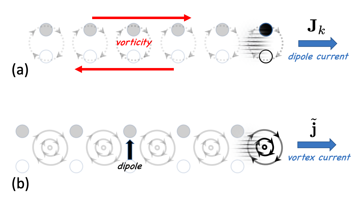
Figure 1: (a) An illustration of a dipole current ${\bf J}_{k}$ transverse to the dipole moment and its equivalence to atomic counter-flow (red arrows) and the associated induced vortex density $\tilde{j}_{0}$. They both contribute to atomic circulation, corresponding to dual charge density of the Gauss’s law (30). (b) An illustration of a vortex current ${\bf j}$ and induced transverse dipole density (black arrow), $J_{0k}$, both contributing to atomic number imbalance, as dual current sources of the Ampere’s law (31).

Finally, to further elucidate Lifshitz model dynamics, I examine the atomic and dipole Ampere’s equations (in real time),

$$\kappa^{-1}{\bm{\nabla}}\times b = -{\partial}_{t}{\bf e}+\tilde{\bf j}-\kappa^{-1}{\bf B}^{*},$$ (31)

$$K^{-1}{\bm{\nabla}}\times B_{k} = -{\partial}_{t}{\bf E}_{k}+\tilde{\bf J}_{k},$$ (32)

corresponding to Lagrangian (22). In (31) I note that the vortex current $\tilde{\bf j}$ induces a dipole density ${\bf B}^{*}_{i}\equiv\epsilon_{ik}B_{k}$ and a gradient in atom density ${\bm{\nabla}}\times b$ transverse to the vortex current. The detailed physical content of this intriguing relation is illustrated in Fig.1(b). I also note that in terms of atomic phase $\phi$, the source-free atomic Ampere’s law just corresponds to a vortex-free condition ${\bm{\nabla}}{\partial}_{t}\phi={\partial}_{t}{\bm{\nabla}}\phi$. This condition is violated by a vortex current $\tilde{\bf j}$ and dipole density ${\bf B}^{*}_{i}$. Equivalently, in terms of atom and dipole densities, in steady state Ampere’s law simply corresponds to force balance between a gradient of the atomic chemical potential (to lowest order the atomic density $n$), a dipole density and the Magnus force associated with the vortex current. I thus observe that Gauss’s and Ampere’s laws illustrate boson-dipole cross-coupling and the associated vortex defects, encoded in the Lagrangian (29), (30).

Summary: In this manuscript I studied phases and phase transitions of a quantum $2+1$d Lifshitz model, a continuum Goldstone-mode field theory of a Bose Hubbard model with dipole conservation.LakeDBHM Reformulating the dipole-conserving second derivative coupling in terms of coupled XY-models of bosons and their dipoles, allows for a description of the phases and transitions in terms of an extension of familiar Bose-condensed and Mott-insulator phases of bosons and dipoles. I complement this direct analysis by a dual coupled gauge theory, that elucidates nontrivial dynamics between bosons, dipoles and their corresponding vortices. It also allows for a transparent description of these transitions as generalized Higgs transitions, whose beyond-mean-field criticality I leave for future studies.

Note Added: After this work was completed I received an interesting preprint from Pranay Gorantla, et al., presenting a complementary lattice duality of a 2+1d compact Lifshitz model, with a detailed treatment of the ground state degeneracy for the periodic boundary conditions.ShuHengLifshitz

Acknowledgments. I thank Shu-Heng Shao and Nati Seiberg for illuminating discussions and for sharing their manuscript before its submission. I appreciate Anton Kapustin’s comments on the manuscript and acknowledge support by the Simons Investigator Award from The James Simons Foundation.

References

- (1) Leo Radzihovsky and Andrey Gromov, Fractonic Matter Reviews of Modern Physics: Colloquia (2022).
- (2) A generalized -Lifshitz model, has elasticity with “soft” (Laplacian) axes and complementary “hard” (gradient) axes. In this nomenclature, the conventional classical 3d smectic is the -Lifshitz model, and 2+1d quantum smectic and 3d classical columnar liquid crystal are described by the -Lifshitz model. Other generalizations include a nonscalar Goldstone mode field as in e.g., tethered membranesJWSmembranes ; LRmembranes ; RTtubulePRL ; RTtubulePRE and nematic elastomersXRelastomers
- (3) Leo Radzihovsky and Tom C. Lubensky, Phys. Rev. E 83, 051701 (2011).
- (4) For a review, and extensive references, see the articles in Statistical Mechanics of Membranes and Interfaces, 2nd edition, Jerusalem Winter School, edited by D. R. Nelson, T. Piran, and S. Weinberg (World Scientific, Singapore, 1989).
- (5) Leo Radzihovsky and John Toner, A New Phase of Tethered Membranes: Tubules Phys. Rev. Lett. 75, 4752 (1995).
- (6) Leo Radzihovsky, John Toner, Elasticity, Shape Fluctuations and Phase Transitions in the New Tubule Phase of Anisotropic Tethered Membranes, Phys.Rev.E 57:1832-1863 (1998).
- (7) Pierre Le Doussal, Leo Radzihovsky, Anomalous elasticity, fluctuations and disorder in elastic membranes, Annals of Physics 392, 340-410 (2018).
- (8) Pierre Le Doussal, Leo Radzihovsky, Thermal Buckling Transition of Crystalline Membranes in a Field, Phys. Rev. Lett. 127, 015702 (2021).
- (9) N. Manoj, R. Moessner, V. B. Shenoy, Tearing Fractons, Phys. Rev. Lett. 127, 067601 (2021).
- (10) Xiangjun Xing, Leo Radzihovsky, Nonlinear Elasticity, Fluctuations and Heterogeneity of Nematic Elastomers, Annals of Physics 323, 105-203 (2008); Universal Elasticity and Fluctuations of Nematic Gels, Phys. Rev. Lett. 90, 168301 (2003).
- (11) P. G. de Gennes and J. Prost, The Physics of Liquid Crystals, 2nd Edition. Clarendon Press, Oxford (1993).
- (12) P. M. Chaikin and T. C. Lubensky, Principles of Condensed Matter Physics, Cambridge (1995).
- (13) M. P. Lilly, K. B. Cooper, J. P. Eisenstein, L. N. Pfeiffer, and K. W. West, Evidence for an anisotropic state of two-dimensional electrons in high Landau levels, Phys. Rev. Lett. 82, 394 (1999).
- (14) A. A. Koulakov, M. M. Fogler, and B. I. Shklovskii, Charge density wave in two-dimensional electron liquid in weak magnetic field, Phys. Rev. Lett. 76, 499 (1996).
- (15) R. Moessner and J. T. Chalker, Exact results for interacting electrons in high Landau levels, Phys. Rev. B 54, 5006 (1996).
- (16) E. Fradkin and S. Kivelson, Liquid-crystal phases of quantum Hall systems , Phys. Rev. B 59, 8065 (1999).
- (17) A. H. MacDonald and Matthew P. A. Fisher, Quantum theory of quantum Hall smectics, Phys. Rev. B 61, 5724 (2000).
- (18) L. Radzihovsky and A. T. Dorsey, Theory of Quantum Hall Nematics, Phys. Rev. Lett. 88, 216802 (2002).
- (19) J. M. Tranquada, et. el., Coexistence of, and competition between, superconductivity and charge-stripe order in LaNdSrCuO, Phys. Rev. Lett. 78, 338 (1997).
- (20) S. A. Kivelson, E. Fradkin, V. J. Emery, Electronic liquid crystal phases of a doped Mott insulator, Nature 393, 550-553 (1998).
- (21) R. Moessner, S. L. Sondhi, and E. Fradkin, Short-ranged resonating valence bond physics, quantum dimer models, and ising gauge theories, Phys. Rev. B 65 (2001).
- (22) A. Vishwanath, L. Balents, and T. Senthil, Quantum criticality and deconfinement in phase transitions between valence bond solids, Physl Rev. B 69
- (23) E. Fradkin, D. A. Huse, R. Moessner, V. Oganesyan, and S. L. Sondhi, Bipartite Rokhsar-Kivelson points and Cantor deconfinement, Phys. Rev. B 69 (2004).
- (24) Vladyslav Kozii, Jonathan Ruhman, Liang Fu, Leo Radzihovsky, Ferromagnetic transition in a one-dimensional spin-orbit-coupled metal and its mapping to a critical point in smectic liquid crystals, Phys. Rev. B 96, 094419 (2017).
- (25) P. Fulde and R.A. Ferrell, Superconductivity in a Strong Spin-Exchange Field, Phys. Rev. 135, A550 (1964).
- (26) A.I. Larkin and Yu. N. Ovchinnikov, Nonuniform state of superconductors, Sov. Phys. JETP 20, 762 (1965).
- (27) L. Radzihovsky and A. Vishwanath, Quantum liquid crystals in an imbalanced Fermi gas: fluctuations and fractional vortices in Larkin-Ovchinnikov states, Phys. Rev. Lett. 103, 010404, (2009).
- (28) L. Radzihovsky, Fluctuations and phase transitions in Larkin-Ovchinnikov liquid-crystal states of a population-imbalanced resonant Fermi gas, Phys. Rev. A. 84, 023611 (2011).
- (29) L. Radzihovsky and S. Choi, P-wave resonant Bose gas: a finite-momentum spinor superfluid, Phys. Rev. Lett. 103, 095302 (2009).
- (30) Hui Zhai, Degenerate quantum gases with spin–orbit coupling: a review, Rep. Prog. Phys. 78, 026001 (2015).
- (31) Tzu-Chi Hsieh, Han Ma, Leo Radzihovsky, Helical superfluid in a frustrated honeycomb Bose-Hubbard model, Phys. Rev. A 106, 023321 (2022).
- (32) G. Grinstein, T. C. Lubensky, and J. Toner, Defect-mediated melting and new phases in three-dimensional systems with a single soft direction, Phys. Rev. B 33, 3306 (1986).
- (33) Leo Radzihovsky, A. M. Ettouhami, Karl Saunders, John Toner, "Soft" Anharmonic Vortex Glass in Ferromagnetic Superconductors, Phys. Rev. Lett., 87, 27001 (2001).
- (34) Karl Saunders, Leo Radzihovsky, John Toner, A Discotic Disguised as a Smectic: A Hybrid Columnar Bragg Glass, Phys. Rev. Lett. 85, 4309 (2000).
- (35) E. Lake, M. Hermele, and T. Senthil, Dipolar Bose-Hubbard model, Phys. Rev. B 106 (2022).
- (36) L. Radzihovsky, Quantum smectic gauge theory, Phys. Rev. Lett. 125, 267601 (2020).
- (37) Z. Z. Zhai and L. Radzihovsky, Fractonic gauge theory of smectics, Annals of Physics 435 (2021) 168509.
- (38) C. Dasgupta and B. I. Halperin, Phase transition in a lattice model of superconductivity, Phys. Rev. Lett. 47, 1556 (1981).
- (39) M. P. A. Fisher and D. H. Lee, Correspondence between two-dimensional bosons and a bulk superconductor in a magnetic field, Phys. Rev. B 39, 2756 (1989).
- (40) J. Beekman, J. Nissinen, K. Wu, K. Liu, R.-J. Slager, Z. Nussinov, V. Cvetkovic, and J. Zaanen, Dual gauge field theory of quantum liquid crystals in two dimensions, Phys. Rep. 683, 1 (2017).
- (41) M. Pretko, Subdimensional particle structure of higher rank U(1) spin liquids. Phys. Rev. B 95, 115139 (2017), arXiv:1604.05329v3
- (42) M. Pretko, Generalized electromagnetism of subdimensional particles. Phys. Rev. B 96, 035119 (2017), arXiv:1606.08857v2
- (43) M. Prekto and L. Radzihovsky, Fracton-elasticity duality, Phys. Rev. Lett. 120, 195301 (2018).
- (44) M. Pretko and L. Radzihovsky, Symmetry-Enriched Fracton Phases from Supersolid Duality, Phys. Rev. Lett. 121, 235301 (2018).
- (45) M. Pretko, Z. Zhai and L. Radzihovsky, Crystal-to-fracton tensor gauge theory dualities, Phys. Rev. B 100, 134113 (2019).
- (46) Ajesh Kumar and Andrew C. Potter, Symmetry-enforced fractonicity and two-dimensional quantum crystal melting, Phys. Rev. B 100, 045119 (2019).
- (47) Andrey Gromov, Chiral topological elasticity and fracton order, Phys. Rev. Lett. 122, 076403 (2019).
- (48) Z. Zhai and L. Radzihovsky, Two-dimensional melting via sine-Gordon duality, Phys. Rev. B 100, 094105 (2019).
- (49) L. Radzihovsky and M. Hermele, Fractons from vector gauge theory, Phys. Rev. Lett. 124, 050402 (2020).
- (50) It is clear from the definition of the boson ) and dipole operators that and are compact angular fields. On a square lattice, where the two lattice vectors have components the minimal coupling reduces to (as usual understood to be regularized by lattice differences inside periodic potential e.g., VillainComment , corresponding to the effective charge , that for simplicity of presentation I took to be .
- (51) This model is quite closely related to that of the quantum smectic, described by the -Lifshitz modelLRsmecticPRL2020 ; ZRsmecticAOP2021 , and also independently appeared in the work of Lake, et al.LakeDBHM .
- (52) The 3d classical nematic-to-smectic phase transition is one of the most enigmatic ones, remaining an open problem, despite extensive theoreticaldeGennes72 ; HLM ; NelsonToner ; Lubensky81 ; TonerNSm ; LRsmecticAerogel and experimentalGarlandExps studies.
- (53) Anton Kapustin and Leo Radzihovsky, Piezosuperconductivity: Novel effects in noncentrosymmetric superconductors, Phys. Rev. B 105, 134514 (2022).
- (54) P. G. DeGennes, An analogy between superconductors and smectics A, Solid State Commun. 10, 753 (1972).
- (55) B. I. Halperin, T. C. Lubensky, and S. K. Ma, First-Order Phase Transitions in Superconductors and Smectic-A Liquid Crystals, Phys. Rev. Lett. 32, 292 (1974).
- (56) D. R. Nelson and J. Toner, Bond-orientational order, dislocation loops, and melting of solids and smectic-A liquid crystals, Phys. Rev. B 24, 363 (1981).
- (57) T. C. Lubensky, S. G. Dunn, Joel Isaacson, Gauge Transformations and the Nematic to Smectic-A Transition, Phys. Rev.Lett. 47, 1609 (1981).
- (58) John Toner, Renormalization-group treatment of the dislocation loop model of the smectic-A nematic transition, Phys. Rev. B 26, 462 (1982).
- (59) Leo Radzihovsky, John Toner, Smectic Liquid Crystals in Random Environments, Phys. Rev. B, 60, 206 (1999).
- (60) C. W. Garland, G. Nounesis, M J. Young, and R. J. Birgeneau, Critical behavior at nematic-smectic-A phase transtions. II. Preasymptotic three-dimensional XY analysis of x-ray and Cp data, Phys. Rev. E 47, 1918 (1993); C. W. Garland and G. Nounesis, Phys. Rev. E 49, 2964 (1994).
- (61) With care of treating compactness of and discreteness of its defects, the continuum approach gives equivalent results to a lattice formulation with compactness encoded via a Villain potential.
- (62) I thus note that “gauging” a model with compact global symmetry thereby takes on a physical content, by making its compactness manifest. The associated field strength is vortex charge and current densities, and gauge redundancy is simply the arbitrariness of division between longitudinal (Goldstone-mode) and transverse (vortex) degrees of freedom.
- (63) Pranay Gorantla, Ho Tat Lam, Nathan Seiberg, and Shu-Heng Shao, 2+1d Compact Lifshitz Theory, Tensor Gauge Theory, and Fractons, preprint.