Tunable superconductivity and Möbius Fermi surfaces
in an inversion-symmetric twisted van der Waals heterostructure

Abstract

We study theoretically a moiré superlattice geometry consisting of mirror-symmetric twisted trilayer graphene surrounded by identical transition metal dichalcogenide layers. We show that this setup allows to switch on/off and control the spin-orbit splitting of the Fermi surfaces via application of a perpendicular displacement field $D_{0}$, and explore two manifestations of this control: first, we compute the evolution of superconducting pairing with $D_{0}$; this features a complex admixture of singlet and triplet pairing and, depending on the pairing state in the parent trilayer system, phase transitions between competing superconducting phases. Second, we reveal that, with application of $D_{0}$, the spin-orbit-induced spin textures exhibit vortices which lead to “Möbius fermi surfaces” in the interior of the Brillouin zone: diabatic electron trajectories, which are predicted to dominate quantum oscillation experiments, require encircling the $\Gamma$ point twice, making their Möbius nature directly observable. We further show that the superconducting order parameter inherits the unconventional, Möbius spin textures. Our findings suggest that this system provides a promising experimental avenue for studying systematically the impact of spin-orbit coupling on the multitude of topological and correlated phases in near-magic-angle twisted trilayer graphene.

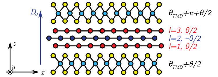
Figure 1: Moiré superlattice studied in this work, which consists of three layers of graphene ($l=1,2,3$) with alternating twist angle $\pm\theta/2$ symmetrically surrounded by TMDs with relative twist angle $\theta_{\text{TMD}}\simeq 30^{\circ}$. A displacement field $D_{0}$ breaks inversion symmetry and, thus, allows to tune the spin-splitting of the bands.

Graphene moiré superlattices MacDonald (2019); Andrei and MacDonald (2020) in the small twist angle regime, $\theta\simeq 1^{\circ}-2^{\circ}$, have emerged in the past few years as a versatile platform for realizing and probing a variety of correlated quantum many-body phases Cao et al. (2018a, b); Yankowitz et al. (2019); Lu et al. (2019); Choi et al. (2019); Kerelsky et al. (2019); Xie et al. (2019); Jiang et al. (2019); Sharpe et al. (2019); Serlin et al. (2020); Cao et al. (2021a); Xie et al. (2021); Rubio-Verdú et al. (2022); Arora et al. (2020); Choi et al. (2021); Lin et al. (2022a); Park et al. (2021); Hao et al. (2021a); Cao et al. (2021b); Kim et al. (2021); Turkel et al. (2022); Liu et al. (2022a); Siriviboon et al. (2021); Lin et al. (2022b); Diez-Merida et al. (2021); Jaoui et al. (2022); Morissette et al. (2022). While the intrinsic spin-orbit coupling (SOC) of graphene is very small Min et al. (2006); Huertas-Hernando et al. (2006), increasing it is expected to enrich the phenomenology of these systems even further: SOC opens up completely new avenues for stabilizing topological phases Hasan and Kane (2010); Wang et al. (2020), is expected to affect the energetic balance of closely competing Kang and Vafek (2019); Xie and MacDonald (2020); Bultinck et al. (2020); Lian et al. (2021); Christos et al. (2022); Wilhelm et al. (2022) instabilities as well as their form Scammell et al. (2022), and has an enormous potential for spintronics applications Sierra et al. (2021); Liu et al. (2022b); Veneri et al. (2022).

Bringing graphene in close proximity to a transition metal dichalcogenide (TMD) layer, which involves heavier atoms, is known to induce SOC Avsar et al. (2014); Wang et al. (2015, 2016); the form of the resultant SOC terms is well established for single-layer Gmitra and Fabian (2015); Li and Koshino (2019); David et al. (2019); Naimer et al. (2021); Lee et al. (2022); Péterfalvi et al. (2022), and non-twisted multi-layer graphene Zollner and Fabian (2021); Zollner et al. (2022). Importantly, the choice of TMD and the twist angle $\theta_{\text{TMD}}$ relative to the proximitzed graphene layer can be used to tune the strength and nature of the induced SOC Naimer et al. (2021); Li and Koshino (2019); David et al. (2019); Lee et al. (2022); Péterfalvi et al. (2022); Zollner and Fabian (2021); Zollner et al. (2022). Although some experiments, see, e.g., Refs. Siriviboon et al., 2021; Lin et al., 2022a, clearly indicate that the proximitized TMD layers influence the correlated physics, in many cases it is not established what role the proximitized TMD layer plays for the observed phases. In general, understanding the impact of SOC on the correlated physics of graphene moiré systems is an open question.

To help elucidate the role of SOC, we here propose and analyze an inversion-symmetric graphene moiré superlattice setup, shown in Fig. 1, which has a key feature that the SOC-induced spin splitting of the Fermi surfaces can be tuned in situ, by applying a perpendicular displacement field $D_{0}$. While the twisted graphene moiré system with the fewest number of layers—twisted bilayer graphene—exhibits spin-split bands already at $D_{0}=0$ Wang et al. (2020), the situation is different for mirror-symmetric twisted trilayer graphene (tTLG): it has inversion symmetry $I$, which persists when being surrounded symmetrically by TMD layers, see Fig. 1; together with time-reversal symmetry, $I$ guarantees pseudospin-degenerate bands, despite the presence of orbital SOC. Breaking it via $D_{0}\neq 0$ allows to tune effective SOC terms lifting the bands’ pseudospin degeneracy.

In this Letter, we study the resulting tunability of the band structure and find that (for $\theta_{\text{TMD}}\simeq 30^{\circ}$) the spin-orbit vector $\bm{g}_{\bm{k}}$ determining the spin-polarizations of the bands exhibits vortices in the interior of the moiré Brillouin zone. These imply that there is a filling fraction—found to be around half filling of the conduction or valence band—with Fermi surfaces that cross each other an odd number of times. We show that this feature can be observed in quantum oscillations where the dominant frequency corresponds to the sum of the inner and outer spin-orbit-split Fermi sheets. To demonstrate the impact of the tunable SOC on the correlated physics of tTLG, we compute the superconducting order parameter as a function of $D_{0}$ assuming different dominant pairing states in the parent tTLG system. We see that $D_{0}$ not only allows to drive superconducting phase transitions and tune the order parameter, it also has the potential of being used as a tool to probe the nature of pairing in tTLG Park et al. (2021); Hao et al. (2021a); Cao et al. (2021b); Kim et al. (2021); Turkel et al. (2022); Liu et al. (2022a); Siriviboon et al. (2021); Lin et al. (2022b), which is currently under debate.

Non-interacting bandstructure.—To model the non-interacting bandstructure of the system in Fig. 1 we use an appropriate generalization of the continuum-model description of twisted bilayer graphene Dos Santos et al. (2007); Bistritzer and MacDonald (2011); Dos Santos et al. (2012); Khalaf et al. (2019); Li et al. (2019); Călugăru et al. (2021). The associated Hamiltonian is diagonal in the graphene layers’ valley degree of freedom, $\eta=\pm$, and consists of four terms, $h_{\eta}=h_{\eta}^{(g)}+h_{\eta}^{(t)}+h^{(\text{SOC})}_{\eta}+h^{(D)}_{\eta}$ See Supplement for more details on the continuum model used, the semi-classical computations of quantum oscillations, and the linearized gap equation . Here $h_{\eta}^{(g)}(\bm{\nabla})$, $\bm{\nabla}=(\partial_{x},\partial_{y})$, and $h_{\eta}^{(t)}(\bm{r})$, $\bm{r}=(x,y)$, capture, respectively, the Dirac cones, rotated by $(-1)^{l}\theta/2$ and with opposite chirality for $\eta=\pm$, of the three layers, $l=1,2,3$, and the tunneling between them, respectively. The latter is spatially modulated on the emergent moiré scale and reconstructs the graphene cones into moiré bands. As a result of the mirror symmetry Khalaf et al. (2019), $\sigma_{h}$, the bandstructure of $h_{\eta}^{(g)}+h_{\eta}^{(t)}$ is that of twisted bilayer graphene ($\sigma_{h}$-even) and single-layer graphene ($\sigma_{h}$-odd bands) in valley $\eta$. Surrounding tTLG with TMD layers as shown in Fig. 1 induces SOC Gmitra and Fabian (2015); Li and Koshino (2019); David et al. (2019); Naimer et al. (2021); Lee et al. (2022); Péterfalvi et al. (2022) in the outer two layers as described by

$$h^{(\text{SOC})}_{\eta}=\sum_{l=1,3}(-1)^{\frac{(l-1)}{2}}P_{l}\left[\lambda_{\text{I}}s_{z}\eta+\lambda_{\text{R}}\left(\eta\rho_{x}s_{y}-\rho_{y}s_{x}\right)\right],$$

where $P_{l}$ projects onto the $l$th graphene layer and $\rho_{j}$ ($s_{j}$), $j=x,y,z$, are Pauli matrices in sublattice (spin) space. The relative minus sign between the $l=1,3$ terms in $h^{(\text{SOC})}_{\eta}$ is dictated by the inversion symmetry, $I$, of the heterostructure. Note that $h^{(\text{SOC})}_{\eta}$ not only breaks spin-rotation symmetry, but also $\sigma_{h}$, which can be seen in the bandstructure shown Fig. 2(a): the graphene Dirac cone of the $\sigma_{h}$-odd sector, located around the $K^{\prime}$ point for the valley shown, hybridizes with the $\sigma_{h}$-even, twisted-bilayer graphene sector. Despite the presence of SOC, all bands are still doubly degenerate, which follows from the momentum-space-local, anti-unitary symmetry $I\Theta_{s}$, with $\Theta_{s}$ being spin-$1/2$ time-reversal, that obeys $(I\Theta_{s})^{2}=-\mathbbm{1}$.

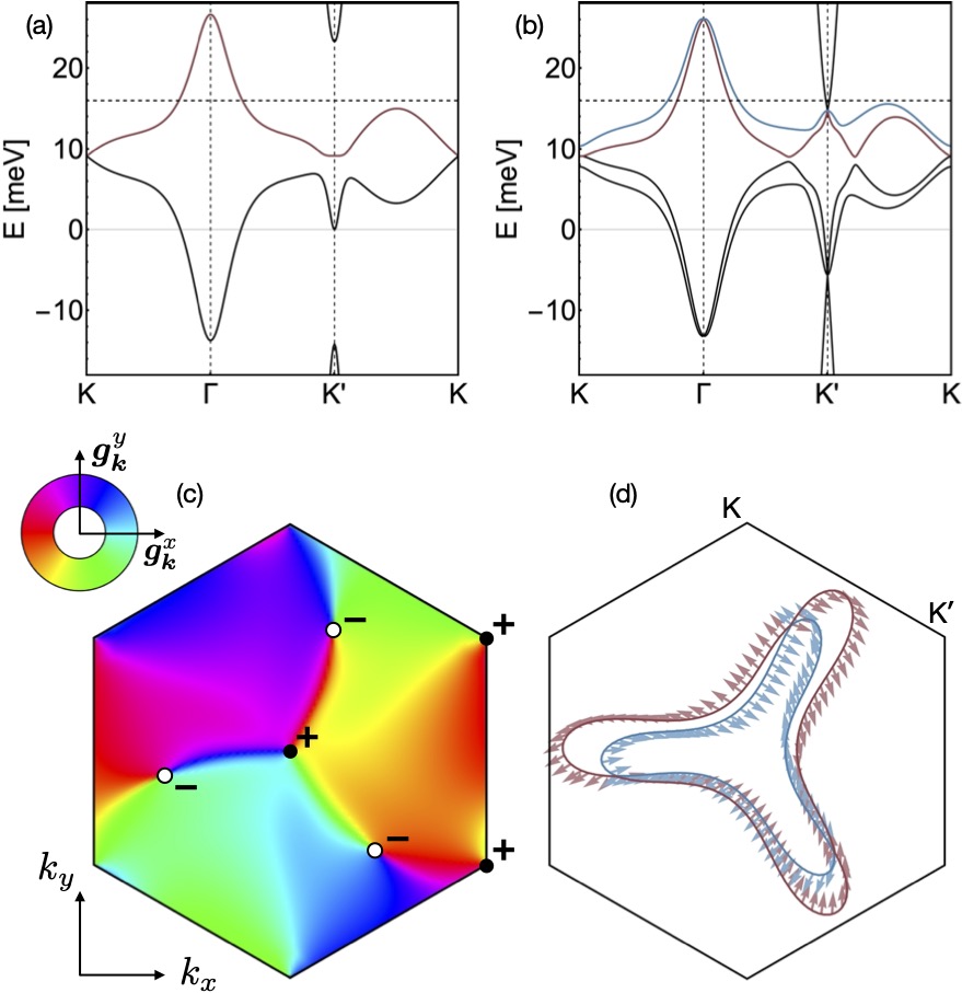
Figure 2: Band structure, including Fermi surfaces and spin texture in valley $\eta=+$. Here twist angle $\theta=1.75^{\circ}$, $\mu=\mu^{*}\simeq 16$ meV, and $\lambda_{\text{R}}=20\,\textrm{meV}$. The cut through the band structure in (a) at $D_{0}=0$ shows spin-degenerate bands. The degeneracy is removed when $D_{0}\neq 0$ as can be seen in (b), where $D_{0}=20\,\textrm{meV}$. Using the same parameters as in (b), the direction of the two non-zero components of $\bm{g}_{\bm{k}}$ in (c) reveals three vortices ($+$) and three anti-vortices ($-$). When $\mu=\mu^{*}$, we obtain vanishing Fermi-surface splitting, see (d), at their $C_{3z}^{s}$-related $\bm{k}$-space locations, leading to a Möbius winding of the spin texture (arrows).

Applying a displacement field $D_{0}$—as is routinely done in experiments on tTLG Park et al. (2021); Hao et al. (2021a); Cao et al. (2021b); Kim et al. (2021); Turkel et al. (2022); Liu et al. (2022a); Siriviboon et al. (2021); Lin et al. (2022b) and captured by the last term, $h^{(D)}_{\eta}$, in the Hamiltonian—breaks $I$ and $I\Theta_{s}$. As such, the pseudospin-degeneracy of the bands at $D_{0}=0$ will be removed when $D_{0}\neq 0$, see Fig. 2(b), providing direct experimental control over the inversion-antisymmetric SOC terms, $\bm{g}_{\bm{k}}\neq 0$, in the effective Hamiltonian, $h^{\text{eff}}_{\bm{k},\eta}=s_{0}\xi_{\eta\cdot\bm{k}}+\eta\,\bm{g}_{\eta\cdot\bm{k}}\cdot\bm{s}$, for the bands of tTLG near the Fermi level. To further discuss the form of $\bm{g}_{\bm{k}}$, let us focus on the limit $\theta_{\text{TMD}}=30^{\circ}$, where $\lambda_{\text{I}}$ vanishes by symmetry Li and Koshino (2019); David et al. (2019); Naimer et al. (2021); Lee et al. (2022) and $(\bm{g}_{\bm{k}})_{z}=0$ as a consequence of $C_{2z}^{s}\Theta_{s}$ ($C_{nz}^{s}$ is the $n$-fold rotation symmetry along $z$). As can be seen in Fig. 2(c), the remaining two components of $\bm{g}_{\bm{k}}$ exhibit vortices at three, $C_{3z}^{s}$-related, generic positions $\bm{k}=\bm{k}^{*}_{j}$, $j=1,2,3$, in the Brillouin zone, compensating those with opposite chirality at $\Gamma$, $K$ and $K^{\prime}$. Since these vortices—and, thus, the associated zeros of $|\bm{g}_{\bm{k}}|$ and type-II Dirac cones in the band structure—cannot be adiabatically removed, we are guaranteed to find a chemical potential $\mu=\mu^{*}$ where the Fermi surface of $\xi_{\bm{k}}$ crosses all three $\bm{k}^{*}_{j}$. For $\mu=\mu^{*}$ ($\mu\simeq\mu^{*}$), the spin-orbit splitting of the Fermi surfaces of the system has to (almost) vanish at these three points, see Fig. 2(d). Having an odd number of points on the Fermi surface where the spin splitting (almost) vanishes also leads to exotic spin textures: following the spin polarizations of the Bloch states [also shown in Fig. 2(d)] diabatically along the Fermi surface, one ends up on the other Fermi sheet after one full revolution, akin to an object traversing a Möbius strip. For this reason and due to the related, but not identical concept of “Möbius fermions” Zhang and Liu (2022), which occur as edge states crossing the zone boundary in systems with non-symmorphic symmetries, we refer to the Fermi surfaces at $\mu=\mu^{*}$ as “Möbius Fermi surfaces”. Note that Möbius Fermi surfaces are only possible since a single valley neither has two-fold out-of-plane rotation nor time-reversal symmetry, which would necessarily lead to an even number of crossing points.

Quantum oscillations.—As our first example of an observable phenomenon associated with these Möbius Fermi surfaces, we discuss quantum oscillations, which are routinely observed in resistivity in small-angle graphene moiré systems Cao et al. (2018a); Phinney et al. (2021); Liu et al. (2022). In the semi-classical picture, the conduction electrons will undergo periodic orbits on quantized constant-energy contours in momentum space when a perpendicular magnetic field $B\neq 0$ is applied. The oscillations of physical quantities are associated with these contours crossing the Fermi level and the frequency $F$ of the oscillations as a function of $1/B$ are proportional to the momentum-space area enclosed by the respective Fermi-surface contours Onsager (1952); Lifshitz and Kosevich (1956).

Let us assume that $\mu$ is close to but not identical to $\mu^{*}$, leading to a finite but small minimal splitting $\delta=|\bm{g}_{\bm{k}_{j}^{*}}|$. In the adiabatic limit at small magnetic fields [$B\ll\delta^{2}/(ev_{g}v_{F})$], the electrons simply follow the outer and inner Fermi surface, indicated as trajectory $\alpha$ and $\beta$ in Fig. 3(b). Meanwhile, finite $B$ will lead to a non-zero transition probability See Supplement for more details on the continuum model used, the semi-classical computations of quantum oscillations, and the linearized gap equation

$$\rho=e^{-\pi\alpha_{B}},\,\,\alpha_{B}=\frac{1}{2}\frac{\delta^{2}}{v_{g}v_{F}}\frac{1}{eB}\left[1+\left(\frac{g\mu_{B}B}{2\delta}\right)^{2}\right],$$ (1)

between the Fermi sheets at each of the three crossing points $\bm{k}=\bm{k}^{*}_{j}$ due to Landau-Zener tunneling Shevchenko et al. (2010); Alexandradinata and Glazman (2018). Here, $v_{F}$ is the Fermi velocity at $\bm{k}=\bm{k}^{*}_{j}$ and $v_{g}=|\partial_{k_{\parallel}}\bm{g}_{\bm{k}_{j}^{*}}|$, with $k_{\parallel}$ denoting the momentum along the Fermi surface. We can see in Fig. 3(d) that $\rho$ reaches a value close to $1$ already at moderately small magnetic fields, $B\gtrsim 10\,\textrm{mT}$, for the values of $v_{g}$, $v_{F}$, $\delta$ extracted from the continuum model at the indicated parameters. At very large magnetic fields, $B\gtrsim 10\,\textrm{T}$, the second term in Eq. (1), which describes the Zeeman-field-induced effective increase of the splitting between the inner and outer Fermi surfaces, starts to dominate and $\rho$ decreases again. Using the frequently applied semi-classical approach Xiao et al. (2010); Alexandradinata and Glazman (2018); Spurrier and Cooper (2019); Mitscherling and Metzner (2021); Paul et al. (2022) and taking into account that intervalley scattering is typically negligible in clean moiré samples Phinney et al. (2021) due to the large momentum-space separation, we computed the Fourier spectrum of quantum oscillations shown in Fig. 3(a). As can be seen most clearly in Fig. 3(c), where the intensities at the frequencies $F_{\mu}$ associated with the fundamental trajectories are shown, there is a large magnetic field range, $0.1-2\,\textrm{T}$, where the Möbius trajectory $\epsilon$ dominates; more precisely, for this field range, which also significantly overlaps with the regime where quantum oscillations are most clearly visible in experiment Phinney et al. (2021), the most prominent fundamental frequency corresponds to the sum of the areas enclosed by the inner and outer Fermi surface—a hallmark signature of its Möbius nature, requiring two revolutions to be closed. In fact, $\epsilon$ is visible and dominant over its constituent trajectories $\alpha$, $\beta$ in most of the experimentally accessible field range. Importantly, the experimental control over $\mu$ allows to adjust $\delta$ which, in turn, determines the magnetic field value $2\delta/g\mu_{B}$ where $\epsilon$ is most prominent; this should facilitate its successful experimental detection. We reiterate that for a Möbius trajectory to dominate quantum oscillations, an odd number of crossing points is required. Setting aside quasi-crystals Spurrier and Cooper (2019) and the case without any rotation symmetry, the single-valley rotation symmetry $C^{s}_{3z}$ of the system is the only possibility to obtain an odd number of crossing points.

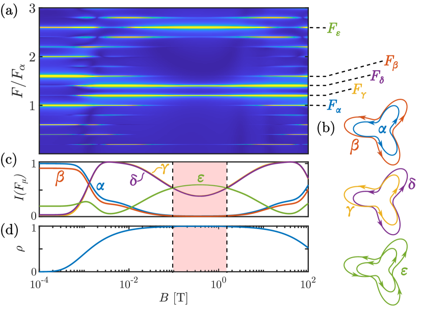
Figure 3: Magnetic field dependence of the quantum oscillation frequency spectrum (a), where we also indicate the frequencies $F_{\mu}$ corresponding to the five orbits $\mu=\alpha,\beta,\gamma,\delta$ depicted in (b). The intensities at these five frequencies and the tunnel probability are plotted in (c) and (d) as a function of magnetic field. In the red region, the Möbius trajectory dominates. The effective parameters entering Eq. (1) have been extracted from the continuum model for $\lambda_{\text{R}}=20\,\textrm{meV}$, $D_{0}=30\,\textrm{meV}$, and $\mu=16.5\,\textrm{meV}$.

Superconductivity.—We now examine the influence of SOC and $D_{0}$ on the superconducting state of tTLG, which we refer to as the parent state. The parent superconducting state comprises Cooper pairs formed from a partially-filled, spin-degenerate band. To be specific, we consider partial filling of the upper moiré bands, c.f. those of Fig. 2(a,b), where also superconductivity is observed experimentally Park et al. (2021); Hao et al. (2021b); Lin et al. (2022b); Siriviboon et al. (2021). Moreover, we exclusively consider intervalley pairing since it is expected Xu and Balents (2018); You and Vishwanath (2019); Scheurer and Samajdar (2020); Lake et al. (2022) to be dominant over intravalley pairing due to time-reversal symmetry $\Theta_{s}$.

To study the evolution of the superconducting state under combined SOC and $D_{0}$ we appeal to the linearized gap equation See Supplement for more details on the continuum model used, the semi-classical computations of quantum oscillations, and the linearized gap equation ,

$$d_{\mu,\bm{k}_{1}}=-\sum_{\bm{k}_{2},\mu^{\prime},\nu}\Gamma_{\mu\mu^{\prime},\bm{k}_{1},\bm{k}_{2}}{\cal W}_{\mu^{\prime}\nu,\bm{k}_{2}}d_{\nu,\bm{k}_{2}},$$ (2)

$${\cal W}_{\mu\nu,\bm{k}}=\sum_{n_{i},s_{j}}\frac{\tanh\left(\frac{\varepsilon_{+,n_{1},\bm{k}}}{2T}\right)+\tanh\left(\frac{\varepsilon_{+,n_{2},\bm{k}}}{2T}\right)}{2(\varepsilon_{+,n_{1},\bm{k}}+\varepsilon_{+,n_{2},\bm{k}})}\times$$

$$(s_{\mu})_{s_{2},s_{3}}C_{+,n_{1},s_{1},\bm{k}}C^{*}_{+,n_{1},s_{2},\bm{k}}C_{+,n_{2},s_{3},\bm{k}}C^{*}_{+,n_{2},s_{4},\bm{k}}(s_{\nu})_{s_{4},s_{1}}.$$

The intervalley superconducting order parameter $d_{\mu,\bm{k}}$ encodes the momentum and spin structure, where $\mu=0$ and $\mu=1,2,3$ refer to the spin-singlet and triplet components, respectively. With perturbed Hamiltonian $h_{\eta}=h^{(g)}_{\eta}+h^{(t)}_{\eta}+h^{(\text{SOC})}_{\eta}+h^{(\text{D})}_{\eta}$, the factors $C^{*}_{\eta,n,s,\bm{k}}\equiv\psi^{\dagger}_{\eta,n,\bm{k}}\psi^{0}_{\eta,s,\bm{k}}$ account for the projection of the perturbed eigenstates $h_{\eta}\psi_{\eta,n,\bm{k}}=\varepsilon_{\eta,n,\bm{k}}\psi_{\eta,n,\bm{k}}$ in band $n$ onto the unperturbed eigenstates $(h^{(g)}_{\eta}+h^{(t)}_{\eta})\psi^{0}_{\eta,s,\bm{k}}=\varepsilon^{0}_{\eta,s,\bm{k}}\psi^{0}_{\eta,s,\bm{k}}$ of spin $s$, which comprise the parent superconducting state. We specialize to $\eta=+$ in (2); the $\eta=-$ order parameter follows from the fermion anticommutation relation. Finally, the interaction vertex $\Gamma_{\mu,\nu,\bm{k}_{1},\bm{k}_{2}}$ assumes an Anderson-Morel-type momentum structure, and encodes the spin-symmetry of the parent state See Supplement for more details on the continuum model used, the semi-classical computations of quantum oscillations, and the linearized gap equation ; we consider three cases: (i) SO(4), (ii) triplet-favored SO(3), and (iii) singlet-favored SO(3), with all states being invariant under $C_{3z}^{s}$ Scheurer and Samajdar (2020).

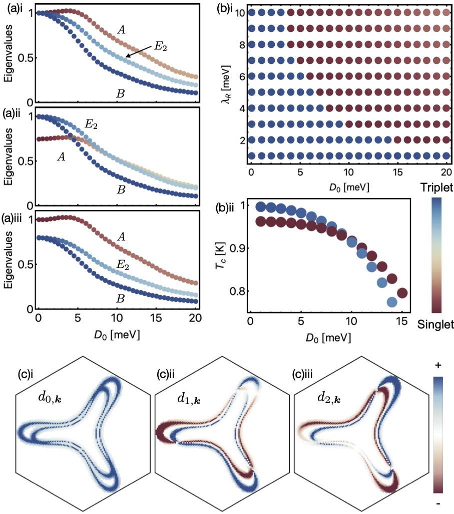
Figure 4: Properties of the superconducting order. (a) Superconducting eigenvalues vs $D_{0}$ [normalized to unity at $D_{0}=0$] and at fixed $\lambda_{\text{R}}=30$ meV. The distinct IRs $(A,B,E_{2})$ of $C_{6}^{s}$ are indicated. The three panels consider different spin-symmetries of the parent state: (ai) SO(4), (aii) triplet-favored SO(3) and (aiii) singlet-favored SO(3). (bi) Phase diagram: colored points mark the dominant IR, with in-plane triplet $E_{2}$ (singlet $A$) state in blue (red). (bii) $T_{c}$ vs $D_{0}$ at $\lambda_{\text{R}}=5$ meV. (c) Order parameter of the leading $A$ state, decomposed into components $d_{\mu,\bm{k}}$; the $\mu=3$ component is zero due to $C_{2z}^{s}$ (not shown). Here $\theta=1.75^{\circ}$ and $\{\lambda_{\text{R}},D_{0}\}=\{20,20\}$ meV [as per Fig. 2(b,c,d)]. The $d_{0,\bm{k}}$ component transforms trivially under $C_{3z}^{s}$, while the admixed in-plane triplet $\bm{d}=(d_{x},d_{y})$ follows a Möbius winding, with $\bm{d}_{\bm{k}}\parallel\bm{g}_{\bm{k}}$.

Having in mind $\theta_{\text{TMD}}\simeq 30^{\circ}$, we focus on $\lambda_{\text{R}}\neq 0$ and $\lambda_{\text{I}}=0$ here. When $D_{0}$ is turned on, the point symmetry is reduced to $C^{s}_{6}$, generated by six-fold out-of-plane rotations. It lacks $I$ and spin-rotation symmetry such that singlet and triplet can mix. More precisely, the parent triplet and singlet phases we consider separate into three distinct superconducting phases when $D_{0}\neq 0$, transforming under the irreducible representations (IRs) $A$, $B$, and $E_{2}$ of $C^{s}_{6}$. Here the $A$ state is predominantly spin-singlet, with admixed in-plane triplet; the $B$ state is pure out-of-plane triplet, since $C^{s}_{2z}$ prohibits any admixture of singlet or in-plane triplet components; and the $E_{2}$ state’s two components are predominantly in-plane triplet, with admixed singlet. At fixed $\lambda_{\text{R}}\neq 0$ we see in Fig. 4(a) that switching on the displacement field $D_{0}$ generates a splitting of these three distinct IRs. Hence, physically, the application of $D_{0}$ allows to change the nature of the superconducting state.

Most strikingly, for the triplet favored parent state, $D_{0}$ drives a phase transition from $E_{2}$ pairing to an $A$ state, as signalled by the crossing of the respective eigenvalues in Fig. 4(a)(ii). This can be more clearly seen in Fig. 4(b)(ii), where we show the changes of the transition temperatures $T_{c}$ corresponding to the eigenvalues of these two states in the vicinity of the transition; both decrease with $D_{0}$ but $T_{c}$ decreases faster for the predominantly triplet state. As expected, the critical value of $D_{0}$ of this transition decreases with increasing $\lambda_{\text{R}}$, see Fig. 4(b)(i).

Finally, we turn to the spin and spatial structure of the superconducting state, encoded in $d_{\mu,\bm{k}}$. Figure 4(c) presents the leading state, $A$. Crucially, we see that the admixed in-plane triplet vector $\bm{d}_{\bm{k}}=(d_{1,\bm{k}},d_{2,\bm{k}})$ behaves as $\bm{d}_{\bm{k}}\parallel\bm{g}_{\bm{k}}$ and has a sign change between the Fermi surfaces; the superconducting order parameter $\bm{d}_{\bm{k}}$ thereby inherits the Möbius winding around the Fermi surface.

Discussion and conclusion.—We showed that the tunable SOC of tTLG with TMD layers on both sides allows to stabilize Möbius-like Fermi surfaces, which result from vortices in the spin texture and are thus of a topological origin. We subsequently proposed quantum oscillations as a smoking gun probe. Turning to superconductivity, we showed that the parent superconducting state of tTLG is readily manipulated in our setup. As only a triplet parent state will give rise to a $D_{0}$-induced superconducting phase transition, this might provide a novel way to access the symmetry of the superconducting state of tTLG. Our analysis can be readily extended to other correlated phases of tTLG, such as magnetic phases or nodal pairing states Scammell and Scheurer (2020) transforming non-trivially under $C_{3z}^{s}$ Scheurer and Samajdar (2020). In conjunction with experimental studies of the geometry in Fig. 1, we believe that this will allow probing the relevance of SOC systematically, e.g., for the stability of superconductivity Arora et al. (2020), for the superconducting diode effect Scammell et al. (2022); Lin et al. (2022b), or the recently observed microwave resonance Morissette et al. (2022) in twisted-graphene-TMD heterostructures.

Appendix A Bandstructure and symmetries

In this appendix, we will first review the continuum model for tTLG, to be self-contained and establish notation. We will then add the proximity-induced SOC terms for the system geometry in Fig. 1, discuss the symmetries, and finally show more details on the resulting band structure.

Continuum model description. To capture the band structure of the system, we use a three-layer extension of the continuum model for twisted-bilayer graphene Dos Santos et al. (2007); Bistritzer and MacDonald (2011); Dos Santos et al. (2012); Khalaf et al. (2019); Li et al. (2019); Călugăru et al. (2021). To write down the Hamiltonian, we define $c_{\bm{k};\rho,l,\eta,s,\bm{G}}$ to be the annihilation operator of an electron in graphene layer $l=1,2,3$ at momentum $\bm{k}$ in the moiré Brillouin zone (MBZ), in sublattice $\rho=A,B$, valley $\eta=\pm$, with spin $s=\uparrow,\downarrow$ and reciprocal moiré lattice (RML) vector $\bm{G}=\sum_{j}n_{j}\bm{G}_{j}$, $n_{j}\in\mathbbm{Z}$. Throughout this work, we use the same symbol for Pauli matrices and the associated quantum numbers; as such, $\rho_{j}$ are Pauli matrices in sublattice, $s_{j}$ in spin, and $\eta_{j}$ in valley space, where $j=0,1,2,3$. To make the mirror symmetry $\sigma_{h}$ of the system more apparent, we go to its eigenbasis Khalaf et al. (2019) by introducing the field operators $\psi_{\bm{k};\rho,\ell,\eta,s,\bm{G}}$ as

$$c_{\bm{k};\rho,l,\eta,s,\bm{G}}=V_{l,\ell}\psi_{\bm{k};\rho,\ell,\eta,s,\bm{G}},\qquad V=\frac{1}{\sqrt{2}}\begin{pmatrix}1&0&-1\\ 0&\sqrt{2}&0\\ 1&0&1\end{pmatrix},$$ (3)

where $\ell=1,2$ and $\ell=3$ refer to the mirror-even and mirror-odd subspaces, respectively.

We split the continuum Hamilton,

$$H_{0}^{\text{Full}}=\sum_{\bm{k}\in\text{MBZ}}\sum_{\rho,\rho^{\prime}=A,B}\sum_{\ell,\ell^{\prime}=1,2,3}\sum_{\eta=\pm}\sum_{s,s^{\prime}=\uparrow,\downarrow}\sum_{\bm{G},\bm{G}^{\prime}\in\text{RL}}\psi^{\dagger}_{\bm{k};\rho,\ell,\eta,s,\bm{G}}\left(h_{\bm{k},\eta}\right)_{\rho,\ell,s,\bm{G};\rho^{\prime},\ell^{\prime},s^{\prime},\bm{G}^{\prime}}\psi^{\phantom{\dagger}}_{\bm{k};\rho^{\prime},\ell^{\prime},\eta,s^{\prime},\bm{G}^{\prime}},$$ (4)

into four parts, $h_{\bm{k},\eta}=h^{(g)}_{\bm{k},\eta}+h^{(t)}_{\bm{k},\eta}+h^{(D)}_{\bm{k}}+h^{(\text{SOC})}_{\bm{k},\eta}$, corresponding to the contribution of the individual graphene layers, the tunneling between the layers, the coupling of the electric displacement field, and the proximity-induced spin-orbit coupling terms. The first term reads as

$$\left(h^{(g)}_{\bm{k},+}\right)_{\rho,\ell,s,\bm{G};\rho^{\prime},\ell^{\prime},s^{\prime},\bm{G}^{\prime}} =\delta_{\ell,\ell^{\prime}}\delta_{s,s^{\prime}}\delta_{\bm{G},\bm{G}^{\prime}}v_{F}(\bm{\rho}_{\theta_{\ell}})_{\rho,\rho^{\prime}}\left(\bm{k}+\bm{G}-(-1)^{\ell}\bm{q}_{1}/2\right),$$ (5)

$$\left(h^{(g)}_{\bm{k},-}\right)_{\rho,\ell,s,\bm{G};\rho^{\prime},\ell^{\prime},s^{\prime},\bm{G}^{\prime}} =\left(h^{(g)}_{-\bm{k},+}\right)^{*}_{\rho,\ell,s,-\bm{G};\rho^{\prime},\ell^{\prime},s^{\prime},-\bm{G}^{\prime}},$$ (6)

where $\bm{\rho}_{\theta}=e^{i\theta\rho_{z}/2}\bm{\rho}e^{-i\theta\rho_{z}/2}$, and $\bm{q}_{1}$ connects the K and K’ points of the MBZ. For the tunneling between the layers, we take the common form

$$\begin{split}\left(h^{(t)}_{\bm{k},+}\right)_{\rho,\ell,s,\bm{G};\rho^{\prime},\ell^{\prime},s^{\prime},\bm{G}^{\prime}}&=\sqrt{2}\,\delta_{s,s^{\prime}}\begin{pmatrix}0&(T_{\bm{G}-\bm{G}^{\prime}})_{\rho,\rho^{\prime}}&0\\ (T_{\bm{G}^{\prime}-\bm{G}}^{*})_{\rho^{\prime},\rho}&0&0\\ 0&0&0\end{pmatrix}_{\ell,\ell^{\prime}},\\ \left(h^{(t)}_{\bm{k},-}\right)_{\rho,\ell,s,\bm{G};\rho^{\prime},\ell^{\prime},s^{\prime},\bm{G}^{\prime}}&=\left(h^{(t)}_{-\bm{k},+}\right)^{*}_{\rho,\ell,s,-\bm{G};\rho^{\prime},\ell^{\prime},s^{\prime},-\bm{G}^{\prime}}.\end{split}$$ (7)

with

$$T_{\delta\bm{G}}=\sum_{j=-1,0,1}\delta_{\delta\bm{G}+\bm{A}_{j},0}\left[w_{0}\rho_{0}+w_{1}\begin{pmatrix}0&\omega^{j}\\ \omega^{-j}&0\end{pmatrix}\right],$$ (8)

$$\omega=e^{i\frac{2\pi}{3}},\quad\bm{A}_{0}=0,\quad\bm{A}_{1}=\bm{G}_{1},\quad\bm{A}_{2}=\bm{G}_{1}+\bm{G}_{2},$$ (9)

which only keeps the lowest-order reciprocal lattice vectors in the Fourier expansion. A finite displacement field leads to the contribution

$$\left(h^{(D)}_{\bm{k}}\right)_{\rho,\ell,s,\bm{G};\rho^{\prime},\ell^{\prime},s^{\prime},\bm{G}^{\prime}}=-D_{0}\delta_{\rho,\rho^{\prime}}\delta_{s,s^{\prime}}\delta_{\bm{G},\bm{G}^{\prime}}\begin{pmatrix}0&0&1\\ 0&0&0\\ 1&0&0\end{pmatrix}_{\ell,\ell^{\prime}}.$$ (10)

Note that the inter-layer tunneling preserves the mirror symmetry, which is why it does not act between the $\ell=1,2$ (even) and $\ell=3$ (odd) sectors in Eq. (7), while $D_{0}$ is odd under it and therefore is entirely off-diagonal in the two sectors, as can be seen in Eq. (10).

Table 1: Action of the point symmetries of the continuum theory on the microscopic field operators $\psi_{\bm{k}}$ defined in Eq. (3) and on the low-energy operators $c_{\bm{k}}$ describing the band structure of the bands that cross the Fermi level via the effective Hamiltonian $H^{\text{eff}}=\sum_{\bm{k}}c^{\dagger}_{\bm{k},\eta}(s_{0}\xi_{\eta\cdot\bm{k}}+\eta\,\bm{g}_{\eta\cdot\bm{k}}\cdot\bm{s})c^{\phantom{\dagger}}_{\bm{k},\eta}$. For convenience of the reader, we also list redundant symmetries. As we are primarily interested in $\lambda_{\text{R}},\lambda_{\text{I}}\gg\lambda_{\text{KM}},m$ Naimer et al. (2021); Li and Koshino (2019); David et al. (2019); Lee et al. (2022); Péterfalvi et al. (2022) and for simplicity, we only state the constraints on $D_{0},\lambda_{\text{R}}$, and $\lambda_{\text{I}}$ for the respective symmetry to be present in the last column while assuming $\lambda_{\text{KM}},m=0$.

Symmetry $S$	unitary?	$S\psi_{\bm{k};\ell,\bm{G}}S^{\dagger}$	$Sc_{\bm{k}}S^{\dagger}$	condition
SO(3)s	✓	$e^{i\bm{\varphi}\cdot\bm{s}}\psi_{\bm{k};\ell,\bm{G}}$	$e^{i\bm{\varphi}\cdot\bm{s}}c_{\bm{k}}$	$\lambda_{\text{R}}=\lambda_{\text{I}}=0$
SO(2)s	✓	$e^{i\varphi s_{z}}\psi_{\bm{k};\ell,\bm{G}}$	$e^{i\varphi s_{z}}c_{\bm{k}}$	$\lambda_{\text{R}}=0$
$C_{3z}$	✓	$e^{i\frac{2\pi}{3}\rho_{z}\eta_{z}}\psi_{C_{3z}\bm{k};\ell,C_{3z}\bm{G}}$	$c_{C_{3z}\bm{k}}$	$\lambda_{\text{R}}=0$
$C^{s}_{3z}$	✓	$e^{i\frac{2\pi}{3}(\rho_{z}\eta_{z}+s_{z})}\psi_{C_{3z}\bm{k};\ell,C_{3z}\bm{G}}$	$e^{i\frac{2\pi}{3}s_{z}}c_{C_{3z}\bm{k}}$	—
$C_{2z}$	✓	$\eta_{x}\rho_{x}\psi_{-\bm{k};\ell,-\bm{G}}$	$\eta_{x}c_{-\bm{k}}$	$\lambda_{\text{R}}=\lambda_{\text{I}}=0$
$C^{s}_{2z}$	✓	$s_{z}\eta_{x}\rho_{x}\psi_{-\bm{k};\ell,-\bm{G}}$	$s_{z}\eta_{x}c_{-\bm{k}}$	$\lambda_{\text{I}}=0$
$C^{s^{\prime}}_{2z}=C^{s}_{2z}is_{y,x}$	✓	$s_{x,y}\eta_{x}\rho_{x}\psi_{-\bm{k};\ell,-\bm{G}}$	$s_{x,y}\eta_{x}c_{-\bm{k}}$	$\lambda_{\text{R}}=0$
$\sigma_{h}$	✓	$(1,1,-1)_{\ell}\psi_{\bm{k};\ell,\bm{G}}$	$\pm c_{\bm{k}}$	$D_{0}=\lambda_{\text{R}}=\lambda_{\text{I}}=0$
$\sigma^{s}_{h}$	✓	$s_{z}(1,1,-1)_{\ell}\psi_{\bm{k};\ell,\bm{G}}$	$\pm s_{z}c_{\bm{k}}$	$D_{0}=\lambda_{\text{I}}=0$
$\sigma^{s^{\prime}}_{h}=\sigma^{s}_{h}is_{y,x}$	✓	$s_{x,y}(1,1,-1)_{\ell}\psi_{\bm{k};\ell,\bm{G}}$	$\pm s_{x,y}c_{\bm{k}}$	$D_{0}=\lambda_{\text{R}}=0$
$I=C_{2z}\sigma_{h}=C^{s}_{2z}\sigma^{s}_{h}$	✓	$\eta_{x}\rho_{x}(1,1,-1)_{\ell}\psi_{-\bm{k};\ell,\bm{G}}$	$\pm\eta_{x}c_{-\bm{k}}$	$D_{0}=0$
$\Theta$	✗	$\eta_{x}\psi_{-\bm{k};\ell,-\bm{G}}$	$\eta_{x}c_{-\bm{k}}$	$\lambda_{\text{R}}=\lambda_{\text{I}}=0$
$\Theta^{s}$	✗	$is_{y}\eta_{x}\psi_{-\bm{k};\ell,-\bm{G}}$	$is_{y}\eta_{x}c_{-\bm{k}}$	—

Finally, let us take into account the additional terms induced by the proximity of the outer two layers to a TMD material, see Fig. 1. To construct the corresponding term, $h^{(\text{SOC})}_{\bm{k}}$, in the Hamiltonian, we start from its form in single-layer graphene Gmitra and Fabian (2015),

$$H_{0,l=1}^{\text{SOC}} =\sum_{\bm{k}\in\text{MBZ}}\sum_{\rho,\rho^{\prime}=A,B}\sum_{\eta=\pm}\sum_{s,s^{\prime}=\uparrow,\downarrow}\sum_{\bm{G}\in\text{RL}}c^{\dagger}_{\bm{k};\rho,1,\eta,s,\bm{G}}\left(h^{\text{SOC},l=1}_{\eta}\right)_{\rho,s;\rho^{\prime},s^{\prime}}c^{\phantom{\dagger}}_{\bm{k};\rho^{\prime},1,\eta,s^{\prime},\bm{G}},$$ (11)

$$h^{\text{SOC},l=1}_{\eta} =\lambda_{\text{I}}s_{z}\eta+\lambda_{\text{R}}e^{-i\phi s_{z}/2}\left(\eta\rho_{x}s_{y}-\rho_{y}s_{x}\right)e^{i\phi s_{z}/2}+\lambda_{\text{KM}}\eta\rho_{z}s_{z}+m\rho_{z}.$$ (12)

The first term, proportional to $\lambda_{\text{I}}$, describes “Ising” SOC (since it is still invariant under a residual SO(2) spin rotation), the second ($\lambda_{\text{R}}$) is the “Rashba” term $\lambda_{\text{R}}$, and the third one ($\lambda_{\text{KM}}$) is usually referred to as “Kane-Mele” Kane and Mele (2005) SOC. Among all terms in Eq. (12), the Kane-Mele term is the only one symmetric under two-fold spinless out-of-plane rotation $C_{2z}$ (with representation $\eta_{x}\rho_{x}$, $\bm{k}\rightarrow-\bm{k}$ in single-layer graphene), while all other three are odd under it. The spin-angle $\phi$, which depends Naimer et al. (2021); Lee et al. (2022); Péterfalvi et al. (2022) on the twist angle $\theta_{\text{TMD}}$ between graphene and the TMD layer, can be set to $\phi=0$ without loss of generality for our analysis, since we can absorb it by performing a global spin rotation along the $s_{z}$ axis. Finally, $m$ captures the fact that the TMD layer breaks $C_{2z}$ such that an imbalance of graphene’s sublattices is allowed by symmetry.

All parameters $\lambda_{\text{I}}$, $\lambda_{\text{R}}$, $\lambda_{\text{KM}}$, and $m$ have been computed in a series of first-principle works Naimer et al. (2021); Li and Koshino (2019); David et al. (2019); Lee et al. (2022); Péterfalvi et al. (2022) and are found to depend crucially on $\theta_{\text{TMD}}$ and the TMD material. Importantly, the TMD-graphene bilayer system exhibits a mirror symmetry at $\theta_{\text{TMD}}=\pi/6$, which implies that both $m$ and $\lambda_{\text{I}}$ vanish. While it is straightforward to also include finite $m$ and $\lambda_{\text{KM}}$ in our analysis, we focus on $m=\lambda_{\text{KM}}=0$ in the main text to keep the discussion concise which is justified as follows: $\lambda_{\text{KM}}$ is universally found to be negligibly small for any $\theta_{\text{TMD}}$ and also $m$ is typically much smaller than $\lambda_{\text{I}}$ and $\lambda_{\text{R}}$, in particular for $\pi/12<\theta_{\text{TMD}}<\pi/6$ Naimer et al. (2021); Li and Koshino (2019); David et al. (2019); Lee et al. (2022); furthermore, Ref. Li and Koshino, 2019 argued that $m$ and $\lambda_{\text{KM}}$ are even required to vanish in an incommensurate TMD-graphene superlattice.

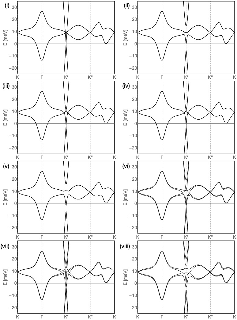
Figure 5: Band structure at twist $\theta=1.75^{\circ}$ for the following combinations of SOC and $D_{0}$: (i) $\lambda_{\text{R}},\lambda_{\text{I}},D_{0}=\{0,0,0\}$meV, (ii) $\lambda_{\text{R}},\lambda_{\text{I}},D_{0}=\{10,0,0\}$meV, (iii) $\lambda_{\text{R}},\lambda_{\text{I}},D_{0}=\{0,10,0\}$meV, (iv) $\lambda_{\text{R}},\lambda_{\text{I}},D_{0}=\{0,0,10\}$meV, (v) $\lambda_{\text{R}},\lambda_{\text{I}},D_{0}=\{10,10,0\}$meV, (vi) $\lambda_{\text{R}},\lambda_{\text{I}},D_{0}=\{10,0,10\}$meV, (vii) $\lambda_{\text{R}},\lambda_{\text{I}},D_{0}=\{0,10,10\}$meV, (viii) $\lambda_{\text{R}},\lambda_{\text{I}},D_{0}=\{10,10,10\}$meV

With $h^{\text{SOC},l=1}_{\eta}$ in Eq. (12) being the coupling in layer $l=1$, the coupling in layer $l=3$ follows by inversion symmetry, $I=C_{2z}\sigma_{h}$,

$$H_{0,l=3}^{\text{SOC}} =\sum_{\bm{k}\in\text{MBZ}}\sum_{\rho,\rho^{\prime}=A,B}\sum_{\eta=\pm}\sum_{s,s^{\prime}=\uparrow,\downarrow}\sum_{\bm{G}\in\text{RL}}c^{\dagger}_{\bm{k};\rho,3,\eta,s,\bm{G}}\left(h^{\text{SOC},l=3}_{\eta}\right)_{\rho,s;\rho^{\prime},s^{\prime}}c^{\phantom{\dagger}}_{\bm{k};\rho^{\prime},3,\eta,s^{\prime},\bm{G}},$$ (13)

$$h^{\text{SOC},l=3}_{\eta} =\rho_{x}h^{\text{SOC},l=1}_{-\eta}\rho_{x}=-\lambda_{\text{I}}s_{z}\eta-\lambda_{\text{R}}\left(\eta\rho_{x}s_{y}-\rho_{y}s_{x}\right)+\lambda_{\text{KM}}\eta\rho_{z}s_{z}-m\rho_{z}.$$ (14)

We assume that there is no direct proximity coupling to the middle layer and, hence, $H_{0,l=2}^{\text{SOC}}$=0. Upon transforming to the mirror eigenbasis according to Eq. (3), we find

$$\left(h^{(\text{SOC})}_{\bm{k},\eta}\right)_{\rho,\ell,s,\bm{G};\rho^{\prime},\ell^{\prime},s^{\prime},\bm{G}^{\prime}}=\delta_{\bm{G},\bm{G}^{\prime}}\begin{pmatrix}(h_{\eta}^{\text{s}})_{\rho,s;\rho^{\prime},s^{\prime}}&0&(h_{\eta}^{\text{a}})_{\rho,s;\rho^{\prime},s^{\prime}}\\ 0&0&0\\ (h_{\eta}^{\text{a}})_{\rho,s;\rho^{\prime},s^{\prime}}&0&(h_{\eta}^{\text{s}})_{\rho,s;\rho^{\prime},s^{\prime}}\end{pmatrix},$$ (15)

where we define the mirror symmetric (s) and anti-symmetric (a) combinations of the individual layer SOC coupling terms,

$$h_{\eta}^{\text{s}} =\frac{1}{2}\left(h^{\text{SOC},l=1}_{\eta}+h^{\text{SOC},l=3}_{\eta}\right)=\lambda_{\text{KM}}\eta\rho_{z}s_{z}$$ (16)

$$h_{\eta}^{\text{a}} =\frac{1}{2}\left(h^{\text{SOC},l=3}_{\eta}-h^{\text{SOC},l=1}_{\eta}\right)=-\lambda_{\text{I}}s_{z}\eta-\lambda_{\text{R}}\left(\eta\rho_{x}s_{y}-\rho_{y}s_{x}\right)-m\rho_{z}$$ (17)

As required by symmetry, the mirror-symmetric (anti-symmetric) combinations appear only on the diagonals within each (off-diagonals between different) mirror-symmetry sectors. This is in line with the observation that the spin-orbit splitting of the Fermi surfaces in Fig. 2(d) tends to be larger in the regions closer to the $K^{\prime}$ point since, for the valley shown, the mirror-even and mirror-odd sectors are closer in energy around $K^{\prime}$ [see Fig. 2(b)]. With this, we have defined all parts of the continuum-model Hamiltonian $H_{0}^{\text{Full}}$ in Eq. (4).

Single-particle symmetries. As it is important for our discussion of superconducting instabilities, we list the point symmetries of the continuum-model Hamiltonian (4) and their representations in Table 1. While there are additional approximate internal symmetries, these are not crucial for our analysis and, hence, not included (we refer to Ref. Christos et al., 2022 where these are discussed for tTLG without SOC, using a notation similar to our notation here). To keep the notation compact, we use the additional superscript $s$ to indicate that the operator involves a spin-space transformation on top of its action in all other quantum numbers—momentum $\bm{k}$, sublattice, layer, and valley. For instance, $C_{3z}$ is just a three-fold rotation along the $z$ direction, leaving the spin unchanged, while $C^{s}_{3z}$ also rotates the spin as indicated.

Most importantly for our analysis: at $D_{0}=0$ there is a $\bm{k}$-local anti-unitary symmetry,

$$I\Theta_{s}=C_{2z}\sigma_{h}\Theta_{s}=\rho_{x}\begin{pmatrix}1&0&0\\ 0&1&0\\ 0&0&-1\end{pmatrix}is_{y}\mathcal{K},$$ (18)

where the $3\times 3$ matrix acts in pseudo-layer (or mirror-eigenvalue) space, with label $\ell$ in Eq. (3), and $\mathcal{K}$ denotes complex conjugation. Importantly, $C_{2z}\sigma_{h}\Theta_{s}$ squares to $-1$ and, hence, guarantees the presence of pseudo-spin-degenerate bands. Obviously, this symmetry is broken at $D_{0}\neq 0$, thus, removing the pseudo-spin degeneracy. As such, we can use $D_{0}$ to turn on and off as well as tune the strength of the spin-orbit splitting of the bands, which can be explicitly seen in Fig. 2 of the main text and Fig. 5 below.

Band structure plots. Figure 5 presents the band structure at twist angle $\theta=1.75^{\circ}$, for various combinations of the SOC parameters $\lambda_{\text{R}},\lambda_{\text{I}}$ and displacement field value $D_{0}$. This illustrates the following expectations based on the symmetries discussed above: first, only if both $D_{0}$ and SOC are finite will the spin degeneracy of the bands be removed—SOC alone is not enough due to the anti-unitary symmetry (18). Second, $\sigma_{h}$ will be broken if one or more of $\{\lambda_{\text{R}},\lambda_{\text{I}},D_{0}\}$ is non-zero, leading to an admixture of the twisted-bilayer-graphene (mirror even) and graphene (mirror-odd) sectors of tTLG graphene.

Appendix B Quantum oscillations

In this section, we first provide more details on how the results of Fig. 3 of the main text are obtained and then explicitly contrast it with the quantum oscillations when the number of avoided crossing points is even.

We here employ a commonly used Xiao et al. (2010); Alexandradinata and Glazman (2018); Spurrier and Cooper (2019); Mitscherling and Metzner (2021); Paul et al. (2022) semi-classical theory that allows to capture the interference effects between the electron trajectories on the outer (red, label $s=+$) and inner (blue, label $s=-$) Fermi surfaces in Fig. 6(a). Let us denote the ($2\times 2$) scattering matrix associated with the avoided crossings $c=1,2,\dots N_{c}$ by $\mathcal{S}^{c}_{s,s^{\prime}}$ and let the phases accumulated on the parts of the Fermi surfaces connecting the scattering regions $c$ and $c^{\prime}$ be on the diagonal of the diagonal matrix $\Lambda^{c\rightarrow c^{\prime}}=\text{diag}(e^{i\Omega_{+}^{c\rightarrow c^{\prime}}},e^{i\Omega_{-}^{c\rightarrow c^{\prime}}})$. Then, demanding that the time evolution of the amplitudes of an electron at the Fermi surfaces be single-valued implies

$$\det\left(U-\mathbbm{1}\right)=0\quad\text{with}\quad U=\prod_{c=1}^{N_{c}}\mathcal{S}^{c}\Lambda^{c\rightarrow c+1\text{mod}N_{c}},$$ (19)

which provides a quantization condition. Throughout this work, we will assume that all segments $c\rightarrow c+1$ and avoided crossings are related by a $C_{N_{c}}$ symmetry and choose a gauge where $\mathcal{S}^{c}=\mathcal{S}$ and $\Lambda^{c\rightarrow c+1\text{mod}N_{c}}=\Lambda$, independent of $c$; in that case, we simply have $U=(\mathcal{S}\Lambda)^{N_{c}}$.

Scattering matrix. The scattering matrix for interband magnetic breakdown is given by Alexandradinata and Glazman (2018)

$$S=\begin{pmatrix}\sqrt{1-\rho^{2}}e^{i\omega(\alpha_{B})}&-\rho e^{i\vartheta}\\ \rho e^{-i\vartheta}&\sqrt{1-\rho^{2}}e^{-i\omega(\alpha_{B})}\end{pmatrix},$$ (20)

where $\rho$ is the Landau-Zener-like tunneling probability,

$$\rho(B)=e^{-\pi\alpha_{B}},\quad\alpha_{B}=\frac{1}{8}\mathcal{A}l_{B}^{2},\quad l_{B}=\frac{1}{\sqrt{eB}},$$ (21)

with $\mathcal{A}$ denoting the area of the rectangle enclosed by the two branches of the Fermi surfaces, see Fig. 6(b), and $B$ the magnetic field. Furthermore, we have $\omega(\alpha_{B})=\alpha_{B}(1-\ln\alpha_{B})+\text{arg}\Gamma(i\alpha_{B})+\pi/4$ in Eq. (20), where $\Gamma$ is the Gamma function. Finally, $\vartheta$ is the phase related to the relative U(1)-gauge freedom between wavefunctions in the two spin-orbit split bands; it is straightforward to check that it will drop out Alexandradinata and Glazman (2018) for closed loops and therefore in the quantization condition (19), as required by gauge invariance.

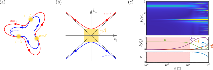
Figure 6: For our semi-classical approach, the Fermi surfaces (red and blue lines) are split into $N_{c}$ segments separated by scattering regions $c=1,2,\dots N_{c}$ (yellow) as shown in (a) for the for us relevant case of $N_{c}=3$. In (b), we display the Fermi surfaces in the immediate vicinity of a scattering region as described by the effective model in Eq. (22). The area $\mathcal{A}$ of the yellow rectangle determines the transition probability via Eq. (21). (c) is the same as Fig. 3(a,c,d) with $\mu$ fine-tuned to $\mu^{*}$ such that the Möbius trajectory also dominates for small magnetic fields.

Importantly, since the states on the two Fermi surfaces that we study have different spin-polarizations, a magnetic field affects $\alpha_{B}$ not only via the (orbital) magnetic length $l_{B}$ but also via the Zeeman field which changes $\mathcal{A}$ in Eq. (21). To study this quantitatively, let us consider a single avoided crossing and denote the deviation of the momentum from the avoided crossing parallel (perpendicular) to the Fermi surfaces right at the avoided crossing point by $k_{\parallel}$ ($k_{\perp}$), see Fig. 6(b). We can then write the effective Hamiltonian in the vicinity of the crossing as

$$h^{\text{eff}}(\bm{k})\sim\sigma_{0}\,v_{F}k_{\perp}+(\sigma_{x},\sigma_{y})^{T}R(\varphi)(v_{g}k_{\parallel},\delta)-\frac{g\mu_{B}}{2}B\sigma_{z},$$ (22)

where $v_{F}$ is the Fermi velocity at the crossing point, $R(\varphi)$ is an O(2) rotation matrix determining the local orientation of the (pseudo)-spin quantum number, $v_{g}$ is the velocity describing the change of the spin-orbit vector with $k$, and $\delta$ its magnitude right at the crossing point ($k_{\parallel}=0$), i.e., the minimal energy separation of the spin-orbit-split bands for $B=0$. Finally, $\mu_{B}=\frac{e}{2m_{e}}$ is the Bohr magneton and $g=2$ the electron’s Landé factor. Computing $\mathcal{A}$ for this model, we get from Eq. (21)

$$\rho(B)=e^{-\pi\alpha_{B}},\quad\alpha_{B}=\frac{1}{2}\frac{\delta^{2}}{v_{g}v_{F}}\frac{1}{eB}\left[1+\left(\frac{g\mu_{B}B}{2\delta}\right)^{2}\right].$$ (23)

As can be seen in Fig. 3(d), this leads to a non-monotonic behavior of $\alpha_{B}$ and, thus, $\rho$ with magnetic field: upon increasing $B$, $\alpha_{B}$ first decreases and reaches its minimum at

$$B_{0}=\frac{2\delta}{g\mu_{B}}\qquad\text{where}\quad\alpha_{B}|_{B=B_{0}}=\frac{\delta}{2m_{e}v_{g}v_{F}}=:\alpha_{0},$$ (24)

before increasing again due to the Zeeman-induced increase of the gap. With this, we can write Eq. (23) in the compact dimensionless form

$$\rho(B)=e^{-\frac{\pi}{2}\alpha_{0}(b+b^{-1})},\qquad b=B/B_{0}.$$ (25)

By fitting the effective Hamiltonian in Eq. (22) to our bandstructure calculations, we find $\delta\simeq 0.022\,\textrm{meV}$, $v_{F}\simeq 0.076v_{0}$, and $v_{g}\simeq 0.02v_{0}$, with $v_{0}$ being the velocity of single-layer graphene, for $\lambda_{\text{R}}=20\,\textrm{meV}$, $D=30\,\textrm{meV}$, and $\mu=16.5\,\textrm{meV}$; this leads to $B_{0}\simeq 0.38\,\textrm{T}$ and $\alpha_{0}=0.0016$, i.e., a maximum tunnel probability of about $0.995$. These are the parameters used in Fig. 3(a,c,d) of the main text.

We note, however, that the value of $\delta$ can be tuned in experiment by gate voltage as it crucially depends on the difference of the chemical potential $\mu$ and the energy $\mu^{*}$ of the vortices in Fig. 2(c). Specifically, by tuning $\mu\rightarrow\mu^{*}$, we obtain $\delta\rightarrow 0$ and, thus,

$$\rho(B)\sim e^{-\pi B/B^{*}},\quad B^{*}=2\left(\frac{2}{g}\right)^{2}\frac{v_{g}v_{F}e}{\mu_{B}^{2}}.$$ (26)

For the parameters above we find $B^{*}\simeq 480\,\textrm{T}$. The associated transition probability looks virtually identical to that shown in Fig. 3(d) of the main text to the right of the red region and indistinguishable from $1$ to the left of it. Consequently, this pushes the lower bound of the magnetic-field range where the Möbius trajectory dominates to zero, as can be seen in Fig. 6(c).

Phases on Fermi segments. For the phase conventions introduced above, the phases accumulated on each of the $C_{N_{c}}$-related outer ($s=+$) and inner ($s=-$) Fermi-surface segments between consecutive scattering regions are given by Alexandradinata and Glazman (2018)

$$\Omega_{s}=\frac{A_{s}l_{B}^{2}}{N_{c}}+\frac{\pi}{N_{c}}+\phi^{s}_{\text{Berry}}(B),\qquad s=\pm,$$ (27)

where $A_{s}$ is the oriented momentum-space area enclosed by the outer $s=+$ (inner $s=-$) Fermi surface. The second term on the right-hand side results from the Maslov phase Keller (1958) for our Fermi surfaces that are deformable into a circle, and the last is the Berry phase contribution for that segment, to be discussed shortly. As a simple consistently check, we first note that the resonance condition (19) becomes equivalent to

$$A_{s}l_{B}^{2}=(2l+1)\pi,\qquad l\in\mathbbm{Z},$$ (28)

for $s=+$ or $s=-$, in the limit without any interband tunneling ($\rho=0$) and setting $\phi^{s}_{\text{Berry}}=0$. This is the classic result of Onsager, Lifshitz, and Kosevich Onsager (1952); Lifshitz and Kosevich (1956).

For a spin texture like the one shown in Fig. 2(d), we have $\phi^{s}_{\text{Berry}}(B=0)=2\pi/N_{c}$ (here with $N_{c}=3$). A finite magnetic field, cants the spin out of plane such that $N_{c}\phi^{s}_{\text{Berry}}(B=0)$ is not an integer multiple of $\pi$. However, the characteristic magnetic field scale where the canting and, thus, the impact on the Berry phase become sizeable is not given by $B_{0}=\delta/\mu_{B}$ but instead by $B^{*}=\delta^{*}/\mu_{B}$ where $\delta^{*}\gg\delta_{0}$ is the typical (as opposed to minimal) splitting between the Fermi surfaces. For our parameters, we find $\delta^{*}$ to be of order of $1.5\,\textrm{meV}$ or $B^{*}\simeq 26\,\textrm{T}$ and, thus, negligible in the important field range centered around $B_{0}$. To check more quantitatively, we use

$$\phi^{s}_{\text{Berry}}(B)=\frac{2\pi}{N_{c}}\left(1-\frac{g\mu_{B}B/2}{\sqrt{(\delta^{*})^{2}+(g\mu_{B}B/2)^{2}}}\right)$$ (29)

in Eq. (27) which is the Berry phase contribution assuming that the splitting of the bands is the same for all momenta on the Fermi surface and given by $\delta^{*}$. Even for $\delta^{*}$ significantly smaller than the estimate above, we did not find any noticeable impact of the field-dependence of the Berry phase on the results presented in this work.

Figure 7: (a) Quantum oscillations frequencies for $N_{c}=3$ as a function of magnetic field $B$ obtained by Fourier transform of Eq. (30) in a finite range of inverse magnetic field centered around $1/B$. We use the parameters stated in the text. The intensity of the Fourier transform (normalized to $1$ at the maximum) at the frequencies associated with the five trajectories $\alpha,\beta,\gamma,\delta,\epsilon$ depicted in Fig. 3(b) are shown in (b). In the upper three panels of (c), we show the intensities in arbitrary units [as in Fig. 3(c)] at the frequencies $F_{1}$ and $F_{2}$ (blue and red) associated with the inner and outer Fermi surface, at the Möbius frequency $F_{1}+F_{2}$ (green), and at all other expected resonance frequencies $[jF_{1}+(N_{c}-j)F_{2}]/N_{c}$, $j=1,2,\dots N_{c}-1$ (black, dashed) for $N_{c}=2,3,6$. We use the same parameters as in Fig. 3 and plot the transition probability (fourth panel) as reference.

Computation of quantum oscillations. To quantify the intensity of the different quantum oscillation frequencies in $1/B$, we use a phenomenological approach similar to Spurrier and Cooper (2019). To construct a signal $I(1/B)$ (mimicking the magnetization’s or resistivity’s oscillatory behavior with magnetic field) that is peaked whenever (19) is obeyed, we use

$$\mathcal{S}(1/B)=\frac{\eta}{|\det\left(U(B)-\mathbbm{1}\right)|^{2}+\eta^{2}},$$ (30)

where $\eta$ is a suitably chosen regularization of the peaks. The quantum oscillation frequency spectra are obtained by Fourier transforming $I(1/B)$ in a finite range $[1/B-\Delta_{B^{-1}},1/B+\Delta_{B^{-1}}]$ of inverse magnetic fields. Using the values for $B_{0}$ and $\alpha_{0}$ derived above, taking $\delta^{*}=10\,\textrm{T}$ and assuming for concreteness that the area enclosed by the inner and outer Fermi surfaces are $30\,\%$ and $40\,\%$ of the area of the MBZ, we find the Fourier spectrum (taking $\Delta_{B^{-1}}=1\,\textrm{T}^{-1}$) shown in Fig. 7(a,b). Note that the frequency associated with the Möbius trajectory is dominant in a wide range of magnetic fields. This includes the largest field we can reach here ($\propto 1/\Delta_{B^{-1}}$). In particular, we cannot present a well-defined spectrum in the regime $B\gtrsim 10\,\textrm{T}$ where the Zeeman effect dominates the transition probability since there are too few oscillations in $\mathcal{S}(1/B)$ in this regime. Although this regime is not of primary interest to our work, we present, for completeness, spectra for it as well in Fig. 3 of the main text [and in Fig. 7(c)]. To be able to do this, we took the limit $A_{s}\rightarrow\infty$ at fixed $A_{+}/A_{-}$ in Fig. 3 where one can keep the value of $B$ fixed at $\bar{B}$ in $\rho(B)$ and $\phi^{s}_{\text{Berry}}(B)$ when Fourier transforming $\mathcal{S}(1/B)$ in a range centered around $1/\bar{B}$; this provides a well defined quantum oscillation spectrum for any magnetic field. Furthermore, comparison of Fig. 3 and Fig. 7(a-b) shows that the two approaches agree well in the relevant regime $B<1/\Delta_{B^{-1}}$.

Other crystalline point groups. The fact that the Möbius trajectory dominates in the large-(orbital)-field limit is a rather unique situation in a 2D crystal; it becomes possible since small-twist-angle graphene moiré systems exhibit well defined valley quantum numbers and, within a single valley, both time-reversal, $\Theta$, and out-of-plane two-fold rotation, $C_{2z}$, symmetry are broken. Either one of these two symmetries would guarantee an even number of avoided crossings and the Möbius trajectory cannot be the dominant one for large orbital magnetic fields where $\rho\rightarrow 1$. In fact, for the same parameters as in Fig. 3 of the main text, we find that the Möbius trajectory does not dominate for any field, see Fig. 7(c), for the other non-trivial rotational symmetries, $C_{2z}$ ($N_{c}=2$), $C_{4z}$ ($N_{c}=4$), and $C_{6z}$ ($N_{c}=6$), in a crystalline system.

Appendix C Superconducting instabilities

Parent superconductivity. We refer to the superconducting state of the unperturbed tTLG system as the parent superconducting state. The parent state is taken to have intervalley pairing, which is expected to dominate over intravalley pairing due to time-reversal symmetry, $\Theta_{s}$, and have either SU(2)${}_{+}\times$SU(2)_-, or reduced SU(2), spin symmetry. These assumptions are consistent with previous works Xu and Balents (2018); You and Vishwanath (2019); Scheurer and Samajdar (2020). Here SU(2)${}_{+}\times$SU(2)_- refers to independent spin rotations in each valley. Finally, it is assumed that the parent superconductivity occurs only in the partially filled, spin-degenerate bands. We will denote by $\varepsilon^{0}_{\eta,s,\bm{k}}$ and $\psi^{0}_{\eta,s,\bm{k}}$ the spin-degenerate bands and corresponding eigenfunctions at the Fermi level of the unperturbed system $(h^{(g)}_{\eta}+h^{(t)}_{\eta})$ with quantum numbers: spin $s$; graphene valley $\eta$; and quasimomenta $\bm{k}$, restricted to the moiré BZ.

Our ansatz for the pairing interaction, in the Cooper-channel, is

$${\cal H}_{int} =\sum_{\bm{k}_{1},\bm{k}_{2}}\sum_{s_{1},s_{2},s_{3},s_{4}}\sum_{\eta=\pm 1}(\Gamma_{\bm{k}_{1},\bm{k}_{2}})_{s_{1},s_{2};s_{3},s_{4}}c_{\eta,s_{1}\bm{k}_{1}}^{\dagger}c_{-\eta,s_{3},-\bm{k}_{1}}^{\dagger}c_{-\eta,s_{4},-\bm{k}_{2}}c_{\eta,s_{2},\bm{k}_{2}},$$

The vertex, $(\Gamma_{\bm{k}_{1},\bm{k}_{2}})_{s_{1},s_{2};s_{3},s_{4}}$, is taken to have spin structure,

$$(\Gamma_{\bm{k}_{1},\bm{k}_{2}})_{s_{1},s_{2};s_{3},s_{4}}=\Gamma^{(1)}_{\bm{k}_{1},\bm{k}_{2}}(\sigma_{0})_{s_{1},s_{3}}(\sigma_{0})_{s_{4},s_{2}}+\Gamma^{(2)}_{\bm{k}_{1},\bm{k}_{2}}\sum_{i=1}^{3}(\sigma_{i})_{s_{1},s_{3}}(\sigma_{i})_{s_{4},s_{2}},$$ (31)

such that $\Gamma^{(1)}_{\bm{k}_{1},\bm{k}_{2}}=\Gamma^{(2)}_{\bm{k}_{1},\bm{k}_{2}}$ [$\Gamma^{(1)}_{\bm{k}_{1},\bm{k}_{2}}\neq\Gamma^{(2)}_{\bm{k}_{1},\bm{k}_{2}}$] gives the SU(2)${}_{+}\times$SU(2)_- [SU(2)] limit. The form of the scalar functions $\Gamma^{(1),(2)}_{\bm{k}_{1},\bm{k}_{2}}$ depends on the explicit pairing mechanism; for simplicity we assume an Anderson-Morel form,

$$\Gamma^{(1)}_{\bm{k}_{1},\bm{k}_{2}} =-(\gamma_{0}+\delta\gamma)\Theta_{\bm{k}_{1};\mu}\Theta_{\bm{k}_{2};\mu},\quad\Gamma^{(2)}_{\bm{k}_{1},\bm{k}_{2}}=-\gamma_{0}\Theta_{\bm{k}_{1};\mu}\Theta_{\bm{k}_{2};\mu},$$ (32)

where $\Theta_{\bm{k};\mu}$ is a step-function such that: $\Theta_{\bm{k};\mu}=1$ for $\bm{k}$ within a radius $\Lambda$ of any Fermi momentum $\bm{k}_{F}$, and $\Theta_{\bm{k};\mu}=0$ elsewhere. The $\Lambda$ acts much like the Debye cut-off. Representative plots of $\Theta_{\bm{k};\mu}$ are shown in Fig. 8. An attractive interaction requires $\gamma_{0}>0$. Meanwhile, the small correction $|\delta\gamma|/\gamma_{0}<1$ distinguishes three cases of the parent superconducting state: (i) $\delta\gamma>0$ favors spin-singlet, (ii) $\delta\gamma<0$ favors spin-triplet, and (iii) for $\delta\gamma=0$, spin-singlet and triplet are degenerate.

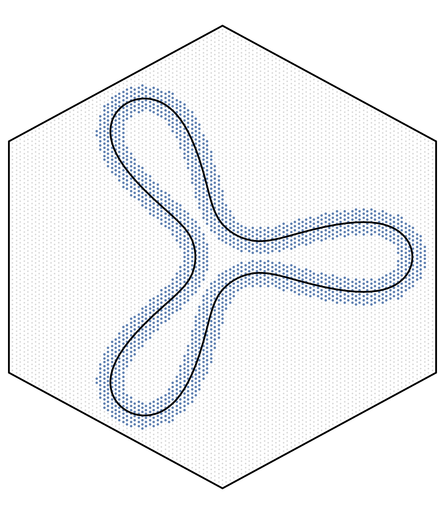
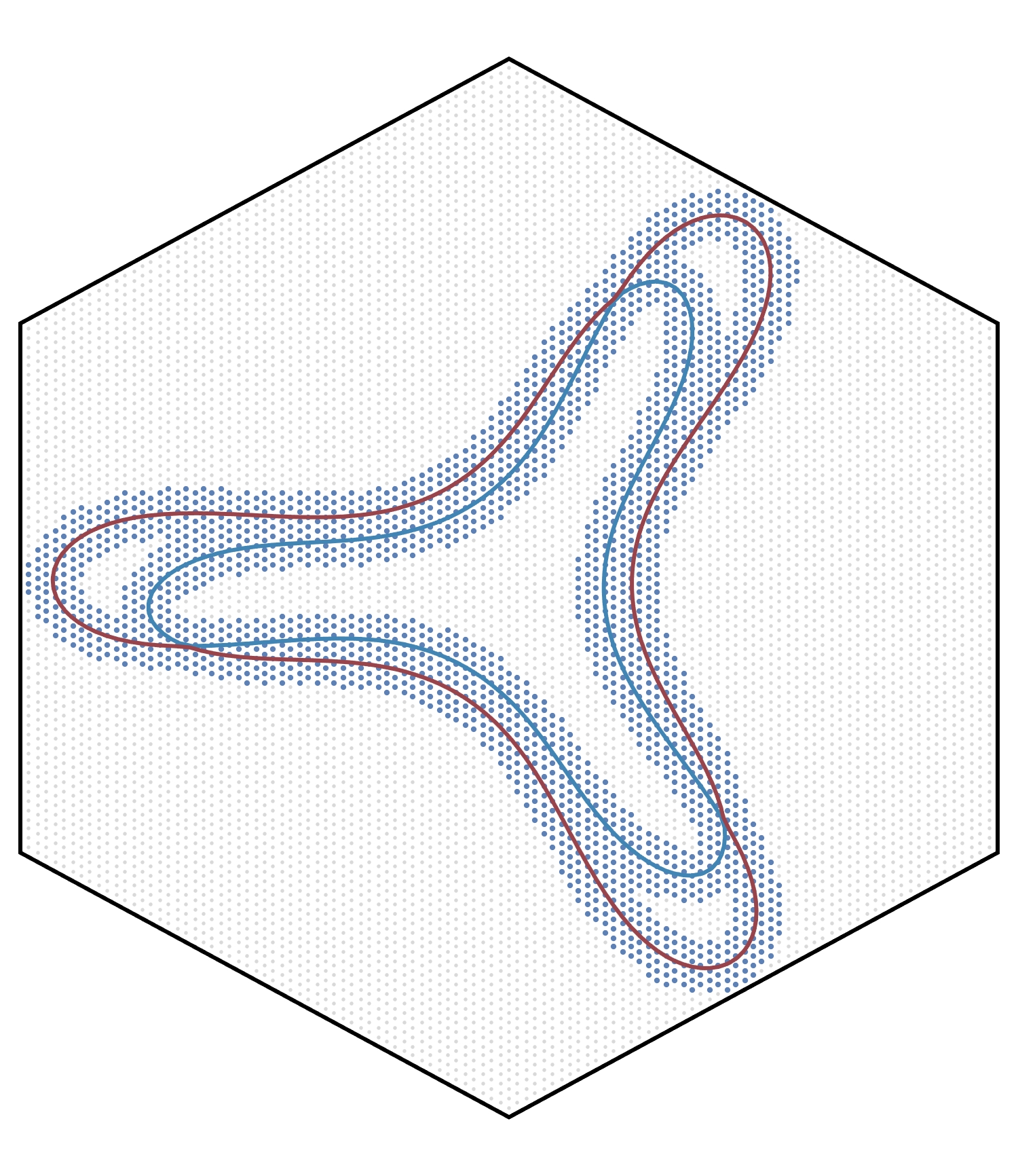
Figure 8: The discrete grid realization of the $\Theta_{\bm{k};\mu}$-functions of (32). Blue points indicate $\Theta_{\bm{k};\mu}=1$, gray points indicate $\Theta_{\bm{k};\mu}=0$. (a) The grid $\Theta_{\bm{k};\mu}$-functions used for computations of Fig. 4; black curve is the Fermi surface of the unperturbed system at $\mu=9.5$ meV (with $\theta=1.50^{\circ}$). (b) Grid $\Theta_{\bm{k};\mu}$-functions used for Fig. 4(c); blue and red curves are the spin-split Fermi surfaces of Fig. 2(d) at $\mu=16$ meV (with $\theta=1.75$).

Perturbed superconductivity. We consider now the evolution of the superconducting order under combined perturbation of SOC and $D_{0}$. In our construction, the perturbations do not influence the vertex $(\Gamma_{\bm{k}_{1},\bm{k}_{2}})_{s_{1},s_{2};s_{3},s_{4}}$, but do still influence the pairing interaction (and hence gap equation) via the perturbed eigenstates of the noninteracting Hamiltonian, $h_{\eta}\psi_{\eta,n,\bm{k}}=\varepsilon_{\eta,n,\bm{k}}\psi_{\eta,n,\bm{k}}$, with $h_{\eta}=h^{(g)}_{\eta}+h^{(t)}_{\eta}+h^{(\text{SOC})}_{\eta}+h^{(\text{D})}_{\eta}$. Here the band index $n$ replaces spin, $s$, which is no longer a good quantum number. Finally, we introduce the electron creation operator $\tilde{c}_{\eta,n,\bm{k}}^{\dagger}$ for the perturbed system, which is related to the unperturbed creation operator via,

$$c^{\dagger}_{\eta,s,\bm{k}}=C^{*}_{\eta,n,s,\bm{k}}\tilde{c}^{\dagger}_{\eta,n,\bm{k}},\quad C^{*}_{\eta,n,s,\bm{k}}\equiv\psi^{\dagger}_{\eta,n,\bm{k}}\psi^{0}_{\eta,s,\bm{k}}.$$ (33)

The mean-field Hamiltonian, decoupled into the Cooper channel for intervalley pairing, is

$${\cal H}_{\eta}=\sum_{\bm{k},n}\varepsilon_{\eta,n,\bm{k}}\tilde{c}_{\eta,n,\bm{k}}^{\dagger}\tilde{c}_{\eta,n,\bm{k}}+\sum_{\bm{k}_{1},\bm{k}_{2}}\sum_{\mu,\nu}(\Gamma^{-1})_{\bm{k}_{1},\bm{k}_{2};\mu,\nu}d_{\mu,\bm{k}_{1},\eta}^{\dagger}d^{\phantom{\dagger}}_{\nu,\bm{k}_{2},\eta}+$$

$$\sum_{\bm{k}}\sum_{n,n^{\prime}}\sum_{s_{1},s_{2}}\sum_{\mu,\nu}\Big{\{}\tilde{c}_{\eta,n,\bm{k}}^{\dagger}\tilde{c}_{\eta,n^{\prime},-\bm{k}}^{\dagger}\left(d_{\mu,\bm{k},\eta}(\sigma_{\mu})_{s_{1},s_{2}}C^{*}_{\eta,n,s_{1},\bm{k}}C_{\eta,n^{\prime},s_{2},\bm{k}}\right)+\text{H.c.}\Big{\}}.$$ (34)

Here the intervalley superconducting order parameter $d_{\mu,\bm{k},\eta}$ encodes the momentum and spin structure of the Cooper pairs, where $\mu=0$ refers to spin-singlet and $\mu=1,2,3$ refer to the components of the spin-triplet. Due to SOC, the $\mu$-components mix as a function of $\bm{k}$; the mixing is encoded in the overlap factors, $C_{\eta,n,s,\bm{k}}$, of Eq. (33). Finally, we introduced the more compact (adjoint) notation $\Gamma_{\bm{k}_{1},\bm{k}_{2};\mu,\nu}\equiv-(\gamma_{0}\delta_{\mu,\nu}+\delta\gamma\delta_{\mu,0}\delta_{\nu,0})\Theta_{\bm{k}_{1};\mu}\Theta_{\bm{k}_{2};\mu}$ and arrive at the linearized gap equation, which follows from (C),

$$d_{\mu,\bm{k}_{1},\eta}=-\sum_{\nu,\bm{k}_{2}}\Gamma_{\mu,\mu^{\prime},\bm{k}_{1},\bm{k}_{2}}{\cal W}_{\mu^{\prime}\nu,\bm{k}_{2},\eta}d_{\nu,\bm{k}_{2},\eta},$$ (35)

$${\cal W}_{\mu\nu,\bm{k},\eta}=\sum_{n_{1},n_{2}}\sum_{s_{1},s_{2},s_{3},s_{4}}\frac{\tanh\left(\frac{\varepsilon_{\eta,n_{1}\bm{k}}}{2T}\right)+\tanh\left(\frac{\varepsilon_{\eta,n_{2}\bm{k}}}{2T}\right)}{2(\varepsilon_{\eta,n_{1}\bm{k}}+\varepsilon_{\eta,n_{2}\bm{k}})}(\sigma_{\mu})_{s_{2},s_{3}}C_{\eta,n_{1},s_{1},\bm{k}}C^{*}_{\eta,n_{1}s_{2},\bm{k}}C_{\eta,n_{2},s_{3},\bm{k}}C^{*}_{\eta,n_{2},s_{4},\bm{k}}(\sigma_{\nu})_{s_{4},s_{1}}.$$

Note that the gap equation is diagonal in $\eta$ and, hence, in the main text we specialized to $\eta=+1$; the $\eta=-1$ order parameter can be subsequently deduced from the fermion anticommutation relation. Using the gap equation in Eq. (35), we compute the evolution of the superconducting order parameters, $d_{\mu,\bm{k},\eta}$, under applied SOC and displacement field, as well as for the different spin-symmetries of the parent superconducting state—encoded in the $\delta\gamma$ of (32)—leading to the results in Fig. 4 of the main text.