On the Effectiveness of Hybrid Pooling in
Mixup-Based Graph Learning for Language Processing

Abstract

Graph neural network (GNN)-based graph learning has been popular in natural language and programming language processing, particularly in text and source code classification. Typically, GNNs are constructed by incorporating alternating layers which learn transformations of graph node features, along with graph pooling layers that use graph pooling operators (e.g., Max-pooling) to effectively reduce the number of nodes while preserving the semantic information of the graph. Recently, to enhance GNNs in graph learning tasks, Manifold-Mixup, a data augmentation technique that produces synthetic graph data by linearly mixing a pair of graph data and their labels, has been widely adopted. However, the performance of Manifold-Mixup can be highly affected by graph pooling operators, and there have not been many studies that are dedicated to uncovering such affection. To bridge this gap, we take an early step to explore how graph pooling operators affect the performance of Mixup-based graph learning. To that end, we conduct a comprehensive empirical study by applying Manifold-Mixup to a formal characterization of graph pooling based on 11 graph pooling operations (9 hybrid pooling operators, 2 non-hybrid pooling operators). The experimental results on both natural language datasets (Gossipcop, Politifact) and programming language datasets (JAVA250, Python800) demonstrate that hybrid pooling operators are more effective for Manifold-Mixup than the standard Max-pooling and the state-of-the-art graph multiset transformer (GMT) pooling, in terms of producing more accurate and robust models.

1 Introduction

Since texts, as well as source code, can be represented as graph-structured data [1, 2], graph neural network (GNN)-based graph learning has been increasingly applied for both natural language processing (NLP) [3], and programming language (PL) understanding [4, 5]. The application of GNNs has achieved remarkable results, e.g., Allamanis et al. [6] utilize GNNs to learn the syntax tree and data flow representations of source code, by which they manage to accomplish several software engineering tasks, such as code completion and defect detection.

Typically, high-quality training data, including features and their corresponding labels, are necessary to train GNN models with competitive performance. However, preparing the labeled data is often not easy, especially in the context of source code labeling that requires advanced expertise [7]. To alleviate the data labeling issue, data augmentation has been proposed to enhance training data by modifying original data. As the state-of-the-art in data augmentation, Mixup [8] achieves impressive results in different tasks. Take image classification for an example: Mixup synthesizes new images and labels as additional training data by first selecting two raw images at random from the original training data and then linearly mixing their features and labels. Recent research [9, 10] demonstrates that Manifold-Mixup, the specialized application of Mixup on graph-structured data [10], can also achieve great performance for graph-structured data. With the success of Manifold-Mixup, utilizing Mixup-based data augmentation in graph learning has emerged as a mainstream paradigm.

As indicated by existing studies [10, 11], Mixup-based graph learning is mainly influenced by two factors, namely, 1) the hyperparameters in Mixup itself, such as the Mixup ratio that balances the proportion of the source data, and 2) the Mixup strategies that are associated with representation generation. Over these factors, the hyperparameter issue is a common one across several different Mixup-applied fields, and has been extensively studied in the fields such as image classification [12, 13]. However, the second issue about Mixup strategies is highly correlated to the context in which Mixup is applied, and for graph-structured data, the influence of such an issue has not been well studied.

In the context of Mixup-based graph learning, as shown in Figure 1, Manifold-Mixup is fed with the inputs from the graph pooling layer, which use graph pooling operators (e.g., Max-pooling) to produce coarsened representations of the given graph while preserve its semantic information. Namely, this layer is the key to representation generation of Manifold-Mixup, in that Manifold-Mixup generate augmented training data by interpolating these representations. Therefore, the performance of Manifold-Mixup can be highly affected by the graph pooling operators. Recent works [14, 15, 16] have attempted to systematically analyze the importance of graph pooling in representation generation; however, the following question, namely, how different graph pooling operators affect the effectiveness of Mixup-based graph learning, still remains open.

In this paper, we tackle this problem by empirically analyzing the difference when Mixup is applied in different graph representations generated by different graph pooling operators. Specifically, we focus on two types of graph pooling methods, namely, standard pooling methods and a unifying formulation of hybrid (mixture) pooling operators. For the standard pooling, the Max-pooling, which is the most widely used one [15], and the state-of-the-art graph multiset transformer pooling (GMT) [17] are considered. For the hybrid pooling, we extend the prior work [16, 18] and design 9 types of hybrid pooling strategies, and more details are introduced in Table 1. Here, GMT and hybrid pooling operators are considered more advanced strategies. We conduct empirical experiments to evaluate the effectiveness of graph learning using Manifold-Mixup [11], under different hybrid pooling operators. In total, our experiments cover diverse types of datasets, including two programming languages (JAVA and Python) and one natural language (English), and consider different tasks, two widely-studied graph-level classification tasks (program classification and Fake news detection), and six GNN model architectures. Based on that, we answer the following research questions:

RQ1: How effective are hybrid pooling operators for enhancing the accuracy of Mixup-based graph learning? The results on NLP datasets (Gossipcop and Politifact used for fake news detection) show that the hybrid pooling operator Type 1 ($\mathcal{M}_{sum}(\mathcal{P}_{att},\mathcal{P}_{max})$) outperforms GMT by up to 4.38% accuracy. On PL datasets (JAVA250 and Python800 used for problem classification), also the hybrid pooling operator Type 1 ($\mathcal{M}_{sum}(\mathcal{P}_{att},\mathcal{P}_{max})$) surpasses GMT by up to 2.36% accuracy.

RQ2: How effective are hybrid pooling operators for enhancing the robustness of Mixup-based graph learning? The results demonstrate that in terms of robustness, the hybrid pooling operator Type 6 ($\mathcal{M}_{concat}(\mathcal{P}_{att},\mathcal{P}_{sum})$) surpasses GMT by up to 23.23% in fake news detection, while the hybrid pooling operator Type 1 ($\mathcal{M}_{sum}(\mathcal{P}_{att},\mathcal{P}_{max})$) outperforms GMT by up to 10.23% in program classification.

RQ3: How does the hyperparameter setting affect the effectiveness of Manifold-Mixup when hybrid pooling operators are applied? According to [8], the hyperparameter $\lambda$ denotes the interpolation ratio, and it is sampled from a Beta distribution with a shape parameter $\alpha\left(\lambda\sim\textit{Beta}\left(\alpha,\alpha\right)\right)$. Existing works [10, 11] show that the hyperparameter setting $\lambda$ affects the performance of Mixup. Therefore, we study the effectiveness of Manifold-Mixup when using hybrid pooling operators under different hyperparameters of Mixup. Experimental results indicate that a smaller value of the hyperparameter leads to better robustness and accuracy.

In summary, the contributions of this paper are as follows:

• This is the first work that explores the potential influence of graph pooling operators on Mixup-based graph-structured data augmentation. To facilitate reproducibility, our code and data are available online.

• We discuss and further extend the hybrid pooling operators from existing works.

• The comprehensive empirical analysis demonstrates that hybrid pooling is a better way for Mixup-based graph-structured data augmentation.

2 Background and Related Work

2.1 Graph Data Classification

Researchers have proposed multiple approaches for the text classification task that analyze the data based on its graph structure. In which Yao et al. [19] constructed text graph data by using the words and documents as nodes. To further enhance text classification performance, Zhang et al. [20] proposed the graph-based word interaction to capture the contextual word relationships. Similar to text data, by capturing the relationship of different components (e.g., variables and operators) in the code, source code data can also be represented structurally as the graph data [5, 21]. Zhou et al. [7] mainly integrated four separate subgraph representations of source code into one joint graph data. Furthermore, to advance the generalization, Allamanis et al. [22] offered four code rewrite rules, such as variable renaming, comment deletion, etc., as a data augmentation for graph-level program classification.

Different from the above works, our study focuses on enhancing the performance of graph classification with Mixup-based data augmentation.

2.2 Graph Pooling Operators

Graph pooling [23, 16] plays a crucial role in capturing relevant structure information of the entire graph. Existing works [24, 25, 26] have proposed the basic graph pooling methods, such as summing or averaging all of the node features. However, such pooling methods treat every node information identically, which could lose the structural information. To solve this problem, researchers [27, 28, 29, 30] dropped nodes with lower scores using a learnable scoring function, which can compress the graph and alleviate the impact of irrelevant nodes to save the important structural information. Additionally, to locate the tightly related communities on a graph, recent works [31, 32, 33, 34] have considered the graph pooling as the node clustering problem, where nodes were specifically aggregated to the same cluster. To combine these advantages, Ranjan et al. [35] first clustered nearby nodes locally and dropped clusters with lower scores. In addition, there existed a kind of attention-based pooling methods [36, 37, 38, 17] that scored nodes with an attention mechanism to weight the relevance of nodes to the current graph-level task. Besides, different from the above standard pooling methods, Nguyen et al. [18] leveraged a mixture of Sum-pooling and Max-pooling methods for graph classification.

In our study, we examine the application of Manifold-Mixup in graph-level classification, incorporating both hybrid pooling and standard pooling techniques.

2.3 Mixup

Due to its effectiveness in graph-structured data processing and the promising performance on graph-specific downstream tasks, e.g., graph classification, GNN has recently received considerable attention. Meanwhile, as a sophisticated data augmentation method, Mixup [8] was initially proposed and implemented within the domain of image classification [39]. Due to its remarkable efficacy in classification tasks, it has subsequently been gradually applied to NLP  [40] and source code learning [10].

In the NLP, Guo et al. [40] proposed two basic strategies of Mixup for augmenting data. One was wording embedding-based, and another was sentence embedding-based. After these two different kinds of embedding, the feature of input data can be mixed to synthesize the new data in vector space. To solve the difficulty in mixing text data in the raw format, Sun et al. [41] mixed text data from transformer-based pre-trained architecture. Chen et al. [42] increased the size of augmented samples by interpolating text data in hidden space. Zhang et al. [43] generated extra labeled sequences in each iteration to augment the scale of training data. Unlike previous work, some researchers considered the raw text itself to augment the input data. Yoon et al. [44] synthesized the new text data from two raw input data by span-based mixing to replace the hidden vectors. In source code learning, Dong et al. [10] proposed a mixup-based data augmentation method that linearly interpolates the features of a pair of programs as well as their labels for the GNN model training.

In our work, we do not simply employ Mixup for graph-structured data classification. Instead, we explore how different graph pooling operators affect the effectiveness of Mixup.

2.4 Empirical Study on Data Augmentation

Recently, there has been a surge of empirical studies exploring the topic of data augmentation. In the NLP, Konno et al. [45] presented an empirical analysis to evaluate the effectiveness of contextual data augmentation (CDA) in improving the quality of the augmented training data, in comparison to [MASK]-based augmentation and linguistically-controlled masking. To assist practitioners in selecting suitable augmentation strategies, Chen et al. [46] conducted a comprehensive empirical study on 11 datasets, encompassing topics such as news classification, inference tasks, paraphrasing tasks, and single-sentence tasks. In source code learning, Yu et al. [47] conducted an empirical study on three program-related downstream tasks, namely method naming, code commenting, and clone detection. The study aimed to validate the effectiveness of data augmentation that is designed by 18 program transformation methods that were preserving both semantics and syntax-naturalness. Dong et al. [21] presented a meticulous empirical study that aimed to evaluate the effectiveness of data augmentation methods that were adapted from the domains of NLP and graph learning for source code learning. The study rigorously examined the impact of these augmentation techniques on enhancing the performance of various tasks related to source code analysis and understanding.

Different from existing empirical studies, our work focuses primarily on examining the influence of graph pooling operators on Mixup-based data augmentation that has received limited attention thus far.

3 Mixup-Based Graph Learning via Hybrid Pooling

3.1 Overview

Figure 1: Overview of Mixup-based graph learning via hybrid pooling.

Figure 1 provides an overview of GNNs for graph classification, demonstrating the application of Manifold-Mixup after the hybrid pooling layer. Concretely, first, GNNs process the input graph-structured data and transform them into node attributes $\left\{x_{i}^{\mathcal{V}}\right\}_{i=1}^{n}$, where $\mathcal{V}$ is the vertex set. Then, after learning the features of each node, the hybrid pooling layer produces the entire graph embedding by utilizing three fundamental types of readout functions: Sum-pooling (SUMPOOL), Max-pooling (MAXPOOL), and Attention-pooling (AttentionPOOL). Finally, as shown in Eq. (1), Manifold-Mixup is applied to randomly mix two selected graph embeddings $\widetilde{{x}_{i}^{\mathcal{G}}}$, $\widetilde{{x_{j}^{\mathcal{G}}}}$ and their ground truth labels ${y_{i}^{\mathcal{G}}}$, ${y_{j}^{\mathcal{G}}}$ with one-hot values as the new training set. This augmented training set is then used for training the classifier. Especially, the utilization of Manifold-Mixup employing the hybrid pooling layer is depicted as follows:

$$\widetilde{x_{mix}^{\mathcal{G}}}=\lambda\widetilde{x_{i}^{\mathcal{G}}}+(1-\lambda)\widetilde{x_{j}^{\mathcal{G}}}$$ (1)

$$y_{mix}^{\mathcal{G}}=\lambda y_{i}^{\mathcal{G}}+(1-\lambda)y_{j}^{\mathcal{G}}$$

where, $\widetilde{x^{\mathcal{G}}}$ is the graph embedding and $y^{\mathcal{G}}$ refers to its label embedding with one-hot value, wherein $\lambda$ means the Mixup ratio. According to [8, 40], $\lambda$ is sampled from a Beta distribution with a shape parameter $\alpha\left(\lambda\sim\textit{Beta}\left(\alpha,\alpha\right)\right)$.

3.2 Graph-level hybrid pooling

In recent research [9], several methods have been proposed to represent graphs at different levels of granularity. These include node-level representation (e.g., node embeddings) and graph-level representation (e.g., graph embeddings), each serving different purposes: node embeddings can be utilized for tasks such as node classification and link prediction, while graph embeddings can be used for graph classification and graph generation [3]. Our work specifically focuses on graph-level representation and its related downstream tasks, e.g., graph classification.

Generally, GNNs learn the graph representation by exploiting the graph structure as an inductive bias, and the GNN architecture proposed by Gilmer et al. [48] is the most popular and widely used in the applications. Briefly speaking, first, given a node with its initialized information, GNN computes the representation by iteratively aggregating its adjacent nodes (Aggregate). Then, it combines this aggregated representation with the existing node representation (Update). After that, a final representation of the complete graph is created by pooling learned features of nodes (Pooling). The primary areas where the various models differ are how they handle aggregation, update, and pooling.

Formally, given a graph-structured data $\mathcal{G}\left(\mathcal{V},\varepsilon\right)$, where $\mathcal{V}$ is the vertex set, and $\varepsilon$ represents the edge set, we simply formulate the entire graph representation $x^{\mathcal{G}}$ as follows:

$$\mathbf{H}_{u}^{k} =\mathbf{GNN}\left(\mathbf{H}_{u}^{k-1},W,\sum_{v\in\mathcal{N}\left(u\right)}\mathbf{H}_{v}^{k-1}\right)$$ (2)

$$\mathbf{H}^{\mathcal{G}} =\mathcal{P}\left(H,\mathcal{V}\right)\quad\text{s.t.}\quad H=\mathbf{H}_{u}^{k}\quad(u\in\mathcal{V})$$

where $\mathbf{H}_{u}^{k-1}$ and $\mathbf{H}_{v}^{k-1}$ denote the matrix representation of node $u$ and $v$ ($u,v\in\mathcal{V}$, $uv\in\varepsilon$) at the $(k-1)$-th iteration, $W$ represents the trainable parameter matrix, $\mathcal{N}\left(u\right)$ is the set of neighbor nodes of $u$, and $\mathcal{P}$ is a graph pooling operator that produces $\mathbf{H}^{\mathcal{G}}$, the latent vector of the entire graph $x^{\mathcal{G}}$. In Eq. 2, firstly, neural network $\mathbf{GNN}\left(\cdot\right)$ is used to iteratively update the latent vector of each node via the message aggregated from the neighborhood $\sum\nolimits_{v\in\mathcal{V}\left(u\right)}\mathbf{H}_{v}^{k-1}$. After that, the pooling operator $\mathcal{P}\left(\cdot\right)$ is used to construct the vector representation of the entire graph, which captures the global information, after $k$ steps of iteration.

In our study, we consider three standard pooling operators $\mathcal{P}$, which are as follows:

$$\mathcal{P}_{att}\left(H,\mathcal{V}\right) =\sum_{u\in\mathcal{V}}\sigma\left(W\mathbf{H}^{k}_{u}+b\right)\odot\phi\left(W\mathbf{H}_{u}^{k}+b\right)$$ (3)

$$\mathcal{P}_{sum}\left(H,\mathcal{V}\right) =\sum_{u\in\mathcal{V}}\mathbf{H}_{u}^{k}$$

$$\mathcal{P}_{max}\left(H,\mathcal{V}\right) =\max_{u\in\mathcal{V}}\mathbf{H}_{u}^{k}$$

where $\phi$ represents the nonlinear activation function, $\odot$ means the Hadamard Product and $\mathbf{H}_{i}^{k}$ refers to the final vector representation of the $i$-th node. Here, $\sigma\left(W\mathbf{H}^{k}_{i}+b\right)$ acts as a soft attention mechanism. We leverage the global attention pooling $\mathcal{P}_{att}$ as it better captures relevant global features for graph-level tasks [36].

Finally, we examine three hybrid pooling functions $\mathcal{M}_{sum}$, $\mathcal{M}_{mul}$ and $\mathcal{M}_{concat}$, defined as follows:

$$\mathcal{M}_{sum}\left(\mathcal{P}_{i},\mathcal{P}_{j}\right) =\mathbf{H}_{\mathcal{P}_{i}}^{\mathcal{G}}+\mathbf{H}_{\mathcal{P}_{j}}^{\mathcal{G}}$$ (4)

$$\mathcal{M}_{mul}\left(\mathcal{P}_{i},\mathcal{P}_{j}\right) =\mathbf{H}_{\mathcal{P}_{i}}^{\mathcal{G}}\odot\mathbf{H}_{\mathcal{P}_{j}}^{\mathcal{G}}$$

$$\mathcal{M}_{concat}\left(\mathcal{P}_{i},\mathcal{P}_{j}\right) =T\left(\left[\mathbf{H}_{\mathcal{P}_{i}}^{\mathcal{G}}\parallel\mathbf{H}_{\mathcal{P}_{j}}^{\mathcal{G}}\right]\right)+b$$

where $\mathbf{H}_{\mathcal{P}_{i}}^{\mathcal{G}}$, $\mathbf{H}_{\mathcal{P}_{j}}^{\mathcal{G}}$ means the embedding vectors of the entire graph, respectively produced by two different pooling operators $\mathcal{P}_{i},\mathcal{P}_{j}$ $(\mathcal{P}_{i}\neq\mathcal{P}_{j})$, as defined in Eq. (3). Here, $\parallel$ denotes the vector concatenation operation, and $T$ is a linear transformation matrix to reduce the dimension $\left(\mathbb{R}^{2d}\rightarrow{\mathbb{R}^{d}}\right)$.

To conclude, the hybrid pooling layer, which consists of the pooling function and pooling operator, can be expressed as follows:

$$\widetilde{{H}^{\mathcal{G}}}=\sum_{u\in\mathcal{V}}\mathcal{M}_{n}(\mathcal{P},H_{u}^{k})$$ (5)

where $\mathcal{M}_{n}\in\left\{\mathcal{M}_{sum},\mathcal{M}_{mul},\mathcal{M}_{concat}\right\}$ and $\widetilde{{H^{\mathcal{G}}}}$ is the matrix representation of the graph data $\mathcal{G}$ produced by the hybrid pooling layer. To more clearly illustrate the design, Table 1 lists the 9 different types of hybrid pooling operators, which are considered in our study.

Table 1: Nine Types of Hybrid Pooling

	Hybrid Pooling Layer
	Pooling Function	Pooling Operator	Description
Type1	$\mathcal{M}_{sum}$	$\mathcal{P}_{att},\mathcal{P}_{max}$	Perform matrix addition on the vectors generated by $\mathcal{P}_{att}$ and $\mathcal{P}_{max}$
Type2	$\mathcal{M}_{mul}$	$\mathcal{P}_{att},\mathcal{P}_{max}$	Perform Hadamard product on the vectors generated by $\mathcal{P}_{att}$ and $\mathcal{P}_{max}$
Type3	$\mathcal{M}_{concat}$	$\mathcal{P}_{att},\mathcal{P}_{max}$	Concatenate the vectors that are generated by $\mathcal{P}_{att}$ and $\mathcal{P}_{max}$
Type4	$\mathcal{M}_{sum}$	$\mathcal{P}_{att},\mathcal{P}_{sum}$	Perform matrix addition on the vectors generated by $\mathcal{P}_{att}$ and $\mathcal{P}_{sum}$
Type5	$\mathcal{M}_{mul}$	$\mathcal{P}_{att},\mathcal{P}_{sum}$	Perform Hadamard product on the vectors generated by $\mathcal{P}_{att}$ and $\mathcal{P}_{sum}$
Type6	$\mathcal{M}_{concat}$	$\mathcal{P}_{att},\mathcal{P}_{sum}$	Concatenate the vectors that are generated by $\mathcal{P}_{att}$ and $\mathcal{P}_{sum}$
Type7	$\mathcal{M}_{sum}$	$\mathcal{P}_{sum},\mathcal{P}_{max}$	Perform matrix addition on the vectors generated by $\mathcal{P}_{sum}$ and $\mathcal{P}_{max}$
Type8	$\mathcal{M}_{mul}$	$\mathcal{P}_{sum},\mathcal{P}_{max}$	Perform Hadamard product on the vectors generated by $\mathcal{P}_{sum}$ and $\mathcal{P}_{max}$
Type9	$\mathcal{M}_{concat}$	$\mathcal{P}_{sum},\mathcal{P}_{max}$	Concatenate the vectors that are generated by $\mathcal{P}_{sum}$ and $\mathcal{P}_{max}$

4 Experimental Setup

4.1 Study Design

To access the effectiveness of hybrid pooling operators in Section 3.2 in Mixup-based graph learning, we design three research questions, as follows:

• RQ1: How effective are hybrid pooling operators for enhancing the accuracy of Mixup-based graph learning? We first explore whether hybrid pooling operators are able to help graph learning with Manifold-Mixup improve the accuracy of GNN models or not. Accuracy which calculates the percentage of correctly identified data among the total number of data in the given test data is the basic metric for evaluating the performance of trained models. Therefore, in this RQ we first evaluate the accuracy performance of hybrid pooling operators (as introduced in Section 3.2) on the NLP binary classification dataset and PL multi-classification dataset, compared to baseline approaches including Max-pooling and the state-of-the-art GMT pooling operators (as introduced in 2.2).

• RQ2: How effective are hybrid pooling operators for enhancing the robustness of Mixup-based graph learning? Robustness is another important metric to reflect the generalization ability of the trained GNN models in practice [49, 50, 51]. In this RQ, we first generate robust test sets by the method [52] that randomly drops the edge-connectivity (i.e., the local connections between a node and its neighboring nodes) of each graph data from the original sets and then calculate the percentage of correctly classified data from this new robust set, to evaluate the robustness of hybrid pooling operators when applied to Mixup-based graph learning [53, 54].

• RQ3: How does the hyperparameter setting affect the effectiveness of Manifold-Mixup when hybrid pooling operators are applied? The hyperparameter $\lambda$ (as introduced in Section 3.1) affects the performance including both accuracy and robustness of Mixup-based graph learning [8, 10, 11]. Therefore, in this RQ we investigate whether this conclusion also holds for Mixup-based graph learning when hybrid pooling operators are applied. Concretely, we evaluate the accuracy and robustness of nine hybrid pooling operators under the setting of the Mixup ratio $\alpha$ from 0.05 to 0.5 in 0.05 intervals.

4.2 Dataset and Model

Dataset. We conduct our study on both traditional NLP and PL tasks. For NLP, we consider User Preference-aware Fake News Detection (UPFD) [55], which is a text-level binary classification problem. For PL, we consider function-level problem multi-classification task provided by Project_CodeNet [56]. Two popular programming languages, Java and Python, are included in our study.

UPFD contains two sets of tree-structured fake and real news propagation graphs that are derived from Twitter. Given a single graph, the source news is represented by the root node, and the leaf nodes represent Twitter users who retweeted the root news. Edges reflect the 1) connection between users and the 2) connection between the user and root news that have been retweeted. Moreover, UPFD also includes 4 different node feature types. These are ➊ Profile feature, a 10-dimensional vector derived from ten user profile attributes; ➋ Spacy feature, a 300-dimensional vector encoded using spacy Word2Vec; ➌ Bert feature, a 768-dimensional vector encoded by BERT (Bidirectional Encoder Representations from Transformers); ➍ Content feature, a 310-dimensional vector obtained by summing the Spacy and Profile features. Fake news detection is commonly approached as a binary classification task, where GNNs provide a negative or positive prediction given a graph of user preferences Project_CodeNet provides two datasets, JAVA250 and Python800. JAVA250 consists of 250 classification problems, and each problem has 300 Java programs. Python800 contains 800 classification problems, and each problem has 300 Python programs. In addition, we transformed the raw source code data from both datasets into a graph representation by utilizing a simplified parse tree. We follow the same process as the original paper to divide the datasets into training, validation, and test sets.

Model. We build 4 different GNN architectures for each dataset. In the text classification, we follow the recommendation of [55] and build Graph Convolution Network (GCN) [57], Graph Isomorphism Network (GIN) [26], Graph Attention Network (GAT) [58], and GraphSAGE [59] models. GCN is a specialized variant of a convolution neural network that is dedicated to operating graph-structured data. GAT mainly uses the attention mechanism for graph message passing. GIN is designed to generalize the Weisfeiler-Lehman (WL) test. GraphSAGE effectively generates node embeddings for previously undiscovered data by utilizing node feature information. In program classification, we use GNN models (GCN, GCN-Virtual, GIN, and GIN-Virtual) provided by [56]. Especially to enhance the aggregation phase of GNNs, virtual nodes, which involve adding an artificial node to each network and connecting it in both directions to all other graph nodes, are offered. To sum up, Table2 shows the details of used datasets and models in our experiment.

Table 2: Details of datasets and DNNs. #Training, #Ori Test, and #Robust Test represent the number of training data, original test data, and test data for generalization evaluation, respectively.

Dataset	Task	#Training	#Clean Test	#Robust Test	Model
Gossipcop	Fake news detection	62	221	314	GCN
					GIN
Politifact	Fake news detection	1092	3826	5464	GAT
					GraphSAGE
JAVA250	Problem classification	48000	15000	75000	GCN
					GCN-Virtual
Python800	Problem classification	153600	48000	240000	GIN
					GIN-Virtual

4.3 Experiment Settings

We implement the hybrid pooling layer based on the open-source library PyG (Pytorch Geometric) [60]. The training epochs we set for Project_CodeNet and UPFD are 100 and 200, respectively. The batch size is set to 80 for Project_CodeNet and 128 for UPFD. For the optimizer, we use Adam [61] with the learning rate $10^{-3}$ for all the models. For Mixup ratio, $\alpha=0.1$ is our default setting. To alleviate overfitting, we adopt early stopping with patience 20. To reduce the impact of randomness, we train each GNN model five times by using different random seeds. We present the average experimental results with standard deviation in the later Section. All the experiments were conducted on a server with 2 GPUs of NVIDIA RTX A6000.

5 Results Analysis

We first study the influence of graph pooling operators on the GNN training with Manifold-Mixup in RQ1 and RQ2, then we go deeper into the hyperparameter settings of Manifold-Mixup in RQ3.

5.1 RQ1: How effective are hybrid pooling operators for enhancing the accuracy of Mixup-based graph learning?

The left part in Table 3 presents the detailed test accuracy results of the GCN model on NLP datasets. From the results, first, we can see that Manifold-Mixup is a powerful technique for augmenting graph-structured data. Compared to the model trained without Manifold-Mixup (No Aug in the tables), GCN model training with data augmentation is more accurate and robust. Then, concerning different pooling operators, we can see that the basic and widely used Max-pooling method (MAXPOOL) and the state-of-the-art GMT pooling operators (GMT) are not the best choices for GCN training with Manifold-Mixup. There are always some hybrid pooling operators that achieve better results than them. More specifically, 8 out of 9 hybrid pooling operators outperform MAXPOOL on the Gossipcop-Profile. Similarly, on the Politifact-Bert, 5 out of 9 hybrid pooling operators achieve higher performance than MAXPOOL. Among these results, the Type 1 operator outperforms GMT by up to 2.14% on Gossipcop and 4.38% on Politifact, respectively. On average, for training with the GCN model, the Type 1 operator demonstrates the best performance under the NLP dataset. Moreover, maybe surprisingly, the gap between using the hybrid pooling operator and MAXPOOL can be up to 2.55% of clean accuracy (Gossipcop, Type1, Profile).

The left part in Table 4 presents the results of the GAT model. Firstly, in both the Gossipcop-Profile and Politifact-Bert datasets, 4 out of the 9 hybrid pooling operators achieve higher test accuracy than MAXPOOL. Moreover, based on the results, the hybrid pooling operator (Type 3) brings the accuracy improvement by up to 2.31% than GMT on the Gossipcop-Spacy, and the operator Type 1 outperforms GMT by up to 2.16% on the Politifact-Content. On average, when training with the GAT model, the hybrid operator (Type 3) proves to be the optimal choice for the PL dataset. It achieves the highest test accuracy on both the Gossipcop and Politifact datasets.

Table 3: Effectiveness of nine types of hybrid pooling w.r.t. test accuracy $\uparrow$ (average $\pm$ standard deviation, %) on original test data and robustness $\uparrow$ (average $\pm$ standard deviation, %) on robust test data of trained GCN models on NLP datasets. No Aug: without Manifold-Mixup data augmentation. A gray background highlights results that are better than MAXPOOL. The best average results are marked in red color.

		Test Accuracy					Robustness
		Profile	Spacy	Bert	Content	Average	Profile	Spacy	Bert	Content	Average
	No Aug	90.48 ± 0.02	96.19 ± 0.07	95.73 ± 0.54	95.44 ± 0.72	94.46	63.19 ± 0.63	85.31 ± 1.73	89.01 ± 0.68	77.17 ± 0.76	78.67
	MAXPOOL	93.17 ± 0.87	96.52 ± 0.09	96.12 ± 0.13	95.79 ± 0.45	95.40	66.97 ± 1.06	86.28 ± 1.21	90.51 ± 0.35	78.98 ± 1.24	80.69
	GMT	93.58 ± 0.32	96.44 ± 0.07	96.25 ± 0.19	96.57 ± 0.02	95.71	75.37 ± 2.93	74.38 ± 0.02	72.39 ± 1.74	94.07 ± 1.11	79.05
	Type1	95.72 ± 0.27	96.84 ± 0.11	96.71 ± 0.26	96.96 ± 0.21	96.56	73.31 ± 1.22	87.58 ± 0.87	91.04 ± 1.25	93.31 ± 0.15	86.31
	Type2	94.11 ± 0.26	95.73 ± 0.24	96.24 ± 0.04	97.36 ± 0.14	95.86	71.77 ± 1.43	72.08 ± 1.22	76.78 ± 1.89	93.36 ± 1.88	78.50
	Type3	95.37 ± 0.33	96.64 ± 0.01	96.63 ± 0.09	96.79 ± 0.13	96.36	67.39 ± 1.65	87.72 ± 2.21	89.99 ± 1.88	83.86 ± 0.12	82.24
	Type4	95.14 ± 0.25	96.28 ± 0.21	94.43 ± 0.59	95.45 ± 0.11	95.33	90.24 ± 0.21	87.33 ± 0.88	77.64 ± 0.95	94.23 ± 1.13	87.36
	Type5	93.64 ± 0.35	96.06 ± 0.04	95.52 ± 0.02	97.04 ± 0.21	95.57	82.91 ± 0.66	86.07 ± 1.88	77.74 ± 0.87	94.17 ± 0.36	85.22
	Type6	93.83 ± 0.18	96.47 ± 0.06	96.58 ± 0.36	95.95 ± 0.25	95.71	80.88 ± 3.29	86.82 ± 1.31	72.99 ± 1.24	74.56 ± 2.75	78.81
	Type7	93.26 ± 0.06	96.25 ± 0.01	95.48 ± 0.04	95.34 ± 0.21	95.08	88.68 ± 3.23	80.66 ± 0.85	71.95 ± 1.18	95.02 ± 0.22	84.08
	Type8	92.12 ± 0.24	95.36 ± 0.13	92.45 ± 0.89	94.07 ± 0.88	93.50	83.61 ± 2.66	84.23 ± 0.72	75.09 ± 2.92	93.44 ± 1.73	84.10
Gossipcop	Type9	93.19 ± 0.05	96.47 ± 0.11	96.03 ± 0.03	95.94 ± 0.13	95.41	88.83 ± 0.16	82.88 ± 3.62	77.66 ± 1.01	94.76 ± 0.47	86.03
	No Aug	77.38 ± 1.81	79.55 ± 1.03	83.15 ± 0.23	84.89 ± 2.51	81.24	64.02 ± 1.59	73.45 ± 0.68	79.63 ± 1.91	81.02 ± 0.66	74.53
	MAXPOOL	77.82 ± 1.26	79.63 ± 0.79	83.49 ± 0.26	85.52 ± 1.22	81.61	66.74 ± 0.32	75.11 ± 0.72	80.09 ± 1.27	82.57 ± 0.95	76.13
	GMT	78.74 ± 0.98	81.46 ± 1.68	84.25 ± 0.81	81.54 ± 1.28	81.50	73.53 ± 4.79	60.27 ± 1.27	79.03 ± 4.61	81.23 ± 0.32	73.52
	Type1	78.96 ± 1.96	81.61 ± 2.49	83.94 ± 0.45	85.92 ± 1.35	82.61	69.01 ± 0.32	74.21 ± 1.12	78.36 ± 2.43	84.84 ± 0.31	76.60
	Type2	77.83 ± 1.64	77.41 ± 2.09	83.72 ± 0.74	85.07 ± 1.09	81.01	68.55 ± 0.96	64.93 ± 0.96	79.86 ± 0.32	82.81 ± 2.56	74.04
	Type3	78.73 ± 2.12	78.88 ± 3.41	83.03 ± 0.58	84.62 ± 1.52	81.31	72.85 ± 0.63	71.71 ± 0.95	80.54 ± 0.63	74.21 ± 1.92	74.83
	Type4	77.22 ± 0.94	81.22 ± 1.86	82.13 ± 3.72	83.37 ± 2.11	80.99	74.43 ± 1.61	75.56 ± 1.27	77.22 ± 3.79	81.67 ± 0.31	77.22
	Type5	77.38 ± 0.46	77.61 ± 1.83	82.24 ± 4.21	82.81 ± 1.27	80.01	71.71 ± 2.24	72.39 ± 0.64	76.41 ± 4.97	81.44 ± 1.27	75.49
	Type6	77.83 ± 1.19	79.31 ± 1.79	84.62 ± 0.98	82.35 ± 1.91	81.03	75.79 ± 0.96	73.75 ± 0.63	82.19 ± 1.45	75.56 ± 3.21	76.82
	Type7	77.08 ± 0.53	80.66 ± 2.85	84.16 ± 0.97	83.03 ± 1.59	81.23	71.49 ± 0.64	71.03 ± 1.28	79.05 ± 4.44	78.28 ± 1.29	74.96
	Type8	78.17 ± 1.49	77.95 ± 0.86	82.02 ± 1.97	83.57 ± 0.64	80.43	68.34 ± 0.87	66.96 ± 3.83	67.64 ± 1.59	74.88 ± 1.61	69.46
Politifact	Type9	78.28 ± 1.36	80.91 ± 1.97	84.39 ± 0.79	84.96 ± 1.29	82.14	76.91 ± 1.27	71.94 ± 1.26	77.37 ± 1.92	84.16 ± 0.63	77.60

The left part in Table 5 presents the results of the PL dataset when training with the GraphSAGE model. Hybrid pooling operators can always help Manifold-mixup in improving test accuracy. For example, in evaluating the performance of hybrid pooling operators, we observe that 4 out of the 9 operators achieve better performance compared with MAXPOOL on both Gossipcop-Profile and Politifact-Bert. Interestingly, while operator Type 1 demonstrates the best performance in most cases, the results from the column Average indicate that operator Type 3 is the optimal choice for the Gossipcop dataset.

Table 4: Effectiveness of nine types of hybrid pooling w.r.t. test accuracy $\uparrow$ (average $\pm$ standard deviation, %) on original test data and robustness $\uparrow$ (average $\pm$ standard deviation, %) on robust test data of trained GAT models on NLP datasets. No Aug: without Manifold-Mixup data augmentation. A gray background highlights results that are better than MAXPOOL. The best average results are marked in red color.

		Test Accuracy					Robustness
		Profile	Spacy	Bert	Content	Average	Profile	Spacy	Bert	Content	Average
	No Aug	91.19 ± 0.03	95.54 ± 0.02	96.49 ± 0.28	97.28 ± 0.43	95.13	90.69 ± 0.21	94.96 ± 0.06	94.49 ± 0.51	96.23 ± 0.63	94.09
	MAXPOOL	93.87 ± 0.47	96.00 ± 0.18	96.74 ± 0.41	97.39 ± 0.24	96.00	90.81 ± 0.52	95.22 ± 0.05	94.53 ± 1.77	96.31 ± 0.89	94.22
	GMT	92.38 ± 0.17	95.96 ± 0.01	95.93 ± 0.39	97.46 ± 0.08	95.43	86.33 ± 2.73	77.44 ± 2.01	79.04 ± 2.06	90.78 ± 3.81	83.40
	Type1	94.68 ± 0.01	96.56 ± 0.31	97.27 ± 0.21	97.54 ± 0.17	96.51	91.89 ± 0.79	95.71 ± 0.59	95.01 ± 2.35	96.82 ± 0.63	94.86
	Type2	94.76 ± 0.54	96.15 ± 0.43	96.99 ± 0.18	97.41 ± 0.09	96.33	91.02 ± 0.52	94.44 ± 1.21	94.95 ± 1.92	96.80 ± 0.49	94.30
	Type3	94.81 ± 0.13	97.08 ± 0.26	97.22 ± 0.16	97.53 ± 0.37	96.66	92.03 ± 0.76	96.46 ± 0.02	93.11 ± 0.91	96.22 ± 0.57	94.46
	Type4	92.57 ± 0.21	95.63 ± 0.02	94.96 ± 0.41	96.71 ± 0.08	94.97	90.68 ± 0.31	94.48 ± 1.03	93.87 ± 0.83	95.53 ± 0.07	93.64
	Type5	92.81 ± 0.59	95.98 ± 0.08	95.42 ± 0.32	97.05 ± 0.31	95.32	90.44 ± 0.46	94.13 ± 0.06	88.23 ± 1.36	95.82 ± 0.74	92.16
	Type6	95.18 ± 0.02	95.94 ± 0.69	96.63 ± 0.81	96.97 ± 0.07	96.18	91.85 ± 018	94.73 ± 0.26	92.75 ± 1.16	96.11 ± 1.19	93.86
	Type7	92.24 ± 0.07	95.23 ± 0.21	94.59 ± 0.04	96.66 ± 0.11	94.68	90.48 ± 0.26	94.07 ± 0.18	93.73 ± 0.95	94.83 ± 0.42	93.28
	Type8	91.92 ± 0.39	95.36 ± 0.47	95.46 ± 0.71	96.39 ± 0.48	94.78	90.24 ± 0.15	94.89 ± 0.41	94.41 ± 0.56	95.87 ± 0.52	93.85
Gossipcop	Type9	92.41 ± 0.09	95.78 ± 0.31	96.04 ± 0.31	97.15 ± 0.04	95.35	90.59 ± 0.11	95.25 ± 0.19	93.98 ± 2.14	96.54 ± 0.43	94.09
	No Aug	74.84 ± 1.38	79.19 ± 0.46	81.61 ± 2.88	85.29 ± 0.58	80.23	74.43 ± 0.32	77.01 ± 1.15	78.28 ± 1.92	84.16 ± 0.64	78.47
	MAXPOOL	75.57 ± 1.11	79.41 ± 0.96	82.58 ± 0.33	85.67 ± 2.14	80.81	75.26 ± 0.69	77.61 ± 0.77	79.54 ± 1.59	84.62 ± 012	79.26
	GMT	76.93 ± 0.46	80.32 ± 0.32	80.54 ± 1.22	83.71 ± 0.63	80.38	74.88 ± 2.87	71.72 ± 0.32	78.43 ± 1.82	81.14 ± 1.59	76.54
	Type1	75.11 ± 0.66	80.41 ± 1.05	83.04 ± 0.31	86.88 ± 0.64	81.36	74.45 ± 0.27	79.05 ± 1.21	81.89 ± 0.64	85.06 ± 1.28	80.11
	Type2	76.17 ± 0.69	79.86 ± 0.32	82.35 ± 0.95	85.52 ± 0.78	80.98	74.66 ± 0.63	78.73 ± 1.07	74.21 ± 0.61	82.57 ± 0.31	77.54
	Type3	78.73 ± 1.19	78.96 ± 0.33	82.21 ± 0.39	85.75 ± 0.98	81.41	76.02 ± 0.63	76.78 ± 0.19	78.27 ± 0.57	81.67 ± 0.32	78.19
	Type4	76.62 ± 2.03	79.04 ± 0.45	80.09 ± 0.22	83.26 ± 1.28	79.75	74.43 ± 1.24	77.59 ± 0.31	78.05 ± 0.96	75.34 ± 0.28	76.35
	Type5	76.61 ± 1.38	78.73 ± 0.53	79.76 ± 0.31	83.67 ± 1.45	79.69	75.46 ± 0.65	75.56 ± 1.92	75.29 ± 1.67	78.95 ± 2.15	76.32
	Type6	75.27 ± 0.94	78.96 ± 0.32	79.19 ± 0.29	83.81 ± 1.12	79.31	72.95 ± 1.26	76.02 ± 3.19	74.88 ± 2.87	81.21 ± 2.24	76.27
	Type7	76.69 ± 1.95	80.32 ± 0.96	81.99 ± 0.11	86.43 ± 0.77	81.36	75.33 ± 0.31	75.56 ± 3.83	79.64 ± 1.28	71.72 ± 0.33	75.56
	Type8	74.78 ± 2.77	79.19 ± 0.64	81.85 ± 0.21	85.35 ± 0.65	80.29	72.62 ± 1.23	75.06 ± 3.13	76.02 ± 2.55	78.95 ± 0.95	75.66
Politifact	Type9	75.08 ± 2.29	80.29 ± 1.08	81.02 ± 0.32	85.92 ± 0.81	80.58	74.45 ± 0.38	76.26 ± 3.75	79.63 ± 1.27	81.22 ± 2.87	77.89

Table 5: Effectiveness of nine types of hybrid pooling w.r.t. test accuracy $\uparrow$ (average $\pm$ standard deviation, %) on original test data and robustness $\uparrow$ (average $\pm$ standard deviation, %) on robust test data of trained GraphSAGE models on NLP datasets. No Aug: without Manifold-Mixup data augmentation. A gray background highlights results that are better than MAXPOOL. The best average results are marked in red color.

		Test Accuracy					Robustness
		Profile	Spacy	Bert	Content	Average	Profile	Spacy	Bert	Content	Average
	No Aug	92.35 ± 0.02	96.53 ± 0.11	96.62 ± 0.02	97.58 ± 0.06	95.77	90.17 ± 0.37	94.68 ± 0.11	95.61 ± 0.32	96.34 ± 0.28	94.20
	MAXPOOL	93.65 ± 0.33	96.79 ± 0.09	96.81 ± 0.01	97.78 ± 0.02	96.26	90.72 ± 0.48	95.01 ± 0.02	95.84 ± 0.14	96.99 ± 0.03	94.64
	GMT	93.31 ± 0.02	94.61 ± 0.02	94.63 ± 0.09	96.71 ± 0.26	94.82	82.18 ± 2.74	84.72 ± 1.93	85.19 ± 2.24	93.31 ± 2.05	86.35
	Type1	94.41 ± 0.11	96.63 ± 0.15	96.88 ± 0.03	97.91 ± 0.03	96.46	94.05 ± 0.49	95.15 ± 0.05	88.89 ± 2.22	97.69 ± 0.09	93.95
	Type2	94.13 ± 0.12	96.48 ± 0.28	96.47 ± 0.18	97.81 ± 0.04	96.22	92.27 ± 0.83	90.08 ± 1.91	91.85 ± 3.39	97.26 ± 0.13	92.87
	Type3	94.81 ± 0.24	96.92 ± 0.07	96.98 ± 0.24	97.71 ± 0.09	96.61	94.24 ± 0.68	95.91 ± 0.09	95.94 ± 0.16	97.47 ± 0.05	95.89
	Type4	93.57 ± 0.55	94.69 ± 0.11	95.47 ± 0.68	96.66 ± 0.14	95.10	92.91 ± 0.51	94.23 ± 0.05	91.07 ± 1.08	92.57 ± 0.07	92.70
	Type5	92.88 ± 0.17	94.68 ± 0.49	95.36 ± 0.46	97.44 ± 0.22	95.09	92.18 ± 0.21	92.67 ± 2.19	93.78 ± 0.84	96.33 ± 0.92	93.74
	Type6	94.38 ± 0.23	95.32 ± 0.41	95.91 ± 0.06	97.73 ± 0.12	95.84	93.65 ± 0.33	94.17 ± 0.34	93.76 ± 2.16	96.64 ± 0.38	94.56
	Type7	92.61 ± 0.08	94.76 ± 0.35	94.05 ± 0.02	95.35 ± 0.08	94.19	91.82 ± 0.73	94.36 ± 0.02	90.99 ± 0.72	92.27 ± 0.04	92.36
	Type8	92.38 ± 0.42	95.71 ± 0.37	94.56 ± 0.56	96.13 ± 0.22	94.70	91.76 ± 0.62	94.43 ± 0.08	93.37 ± 0.06	94.77 ± 0.09	93.58
Gossipcop	Type9	93.12 ± 0.16	95.92 ± 0.18	94.90 ± 0.68	96.65 ± 0.32	95.15	92.45 ± 0.43	94.39 ± 0.06	92.35 ± 0.46	94.52 ± 0.19	93.43
	No Aug	77.65 ± 1.52	80.27 ± 0.99	82.53 ± 1.96	83.84 ± 1.32	81.07	76.47 ± 0.45	78.05 ± 0.95	80.31 ± 1.59	81.91 ± 1.28	79.19
	MAXPOOL	77.83 ± 0.64	80.54 ± 0.72	83.26 ± 0.96	85.37 ± 0.88	81.75	76.82 ± 0.42	78.51 ± 0.96	82.12 ± 0.31	82.12 ± 0.31	79.89
	GMT	77.15 ± 0.33	79.19 ± 1.25	84.01 ± 0.94	84.11 ± 1.05	81.12	71.94 ± 0.57	65.61 ± 3.21	81.44 ± 0.79	78.06 ± 0.95	74.26
	Type1	78.89 ± 1.88	80.69 ± 0.95	83.71 ± 0.45	86.27 ± 0.94	82.39	77.37 ± 0.63	79.86 ± 0.33	81.67 ± 2.23	85.29 ± 0.91	81.05
	Type2	77.61 ± 0.32	80.59 ± 1.19	82.13 ± 1.59	84.73 ± 2.23	81.27	76.94 ± 1.19	76.46 ± 0.64	81.21 ± 0.32	82.35 ± 2.07	79.24
	Type3	78.73 ± 0.67	80.43 ± 1.17	82.96 ± 0.53	84.71 ± 3.31	81.71	75.33 ± 2.24	79.18 ± 0.63	81.89 ± 0.65	82.34 ± 1.26	79.69
	Type4	77.23 ± 0.55	80.66 ± 0.67	84.01 ± 0.94	83.76 ± 0.02	81.42	75.79 ± 0.33	79.41 ± 0.96	80.99 ± 2.56	74.88 ± 0.33	77.77
	Type5	76.89 ± 0.99	80.32 ± 0.89	82.58 ± 1.23	81.86 ± 0.12	80.41	75.56 ± 1.27	74.66 ± 1.29	80.84 ± 1.46	76.71 ± 3.52	76.94
	Type6	76.57 ± 0.23	80.09 ± 0.63	83.27 ± 1.21	83.26 ± 0.22	80.80	73.98 ± 1.59	76.69 ± 2.24	79.18 ± 1.92	78.28 ± 2.56	77.03
	Type7	76.93 ± 1.28	79.37 ± 1.27	82.21 ± 1.14	82.81 ± 0.11	80.33	71.72 ± 0.32	78.28 ± 0.61	78.28 ± 0.61	73.53 ± 0.85	75.45
	Type8	76.71 ± 0.97	80.55 ± 1.46	81.91 ± 1.28	84.39 ± 0.33	80.89	74.21 ± 1.17	78.96 ± 0.31	78.96 ± 0.31	75.86 ± 2.14	77.00
Politifact	Type9	76.69 ± 0.32	80.47 ± 1.02	84.16 ± 0.78	85.31 ± 0.32	81.66	75.56 ± 0.66	79.63 ± 0.67	83.48 ± 0.28	76.92 ± 3.19	78.90

The left part in Table 6 is the results of the GIN model. Surprisingly, in all cases examined, both operator Type 1 and operator Type 3 consistently outperform MAXPOOL on both the Gossipcop and Politifact datasets. Compared with GMT, the operator Type 1 improves the accuracy by up to 2.10% in Gossipcop-Profile and 1.58% on the Politifact-Bert, respectively. Also, results from the column Average show that the operator Type 1 is still the best choice for both the Gossipcop and Politifact datasets.

Table 7 presents the results of PL datasets. We can see that the advanced graph pooling operators, including GMT and hybrid pooling operators, are more helpful than the MAXPOOL for Mainfold-Mixup when dealing with PL data, where the best results are always from the hybrid pooling operators. Similar to the results of traditional NLP datasets, the Type 1 hybrid pooling operator outperforms MAXPOOL in most situations (6 out of 8 cases). Unlike the NLP datasets, the operator Type 3 consistently achieves better results than MAXPOOL. In PL datasets, the gap between using GMT and hybrid pooling operators can be up to 2.36% of clean accuracy (GIN-Virtural, Python800, Type 1).

From the results of both traditional NLP datasets and PL datasets, we can conclude that hybrid pooling operators have a significant impact on the effectiveness of the Mixup data augmentation technique when dealing the graph-structured datasets. The operator Type 1 ($\mathcal{M}_{sum}(\mathcal{P}_{att},\mathcal{P}_{max})$) is the best choice among our considered candidates in terms of accuracy and is recommended to be used in the graph classification task.

Answer to RQ1: Hybrid pooling operators have a significant impact in enhancing the effectiveness of Manifold-Mixup-based graph learning in terms of clean accuracy. Notably, compared to GMT, the Type 1 operator ($\mathcal{M}_{sum}(\mathcal{P}_{att},\mathcal{P}_{max})$) demonstrates up to 4.38% accuracy improvements on the NLP dataset and 2.36% on the PL dataset, respectively.

5.2 RQ2: How effective are hybrid pooling operators for enhancing the robustness of Mixup-based graph learning?

The right part in Table 3 presents the results of the robustness of the GCN model on the NLP dataset. Firstly, it is observed that Manifold-Mixup significantly enhances the generalization ability of the GNN model. In addition, although GMT is an advanced graph pooling operator, it is unable to help Manifold-Mixup effectively enhance the robustness of the GCN model. It proves to be effective in only 3 out of 8 cases. Then, concerning hybrid pooling operators, surprisingly, all operators obtain better performance in improving the robustness than MAXPOOL on the Gossipcop-Profile and Politifact-Profile datasets. Furthermore, in terms of robustness, the operator Type 9 outperforms GMT by a significant margin of up to 13.46% (Gossipcop-Profile), and the operator Type 4 obtains an even higher improvement in robustness by up to 15.29% (Politifact-Spacy) compared to GMT.

Table 6: Effectiveness of nine types of hybrid pooling w.r.t. test accuracy $\uparrow$ (average $\pm$ standard deviation, %) on original test data and robustness $\uparrow$ (average $\pm$ standard deviation, %) on robust test data of trained GIN models on NLP datasets. No Aug: without Manifold-Mixup data augmentation. A gray background highlights results that are better than MAXPOOL. The best average results are marked in red color.

		Test Accuracy					Robustness
		Profile	Spacy	Bert	Content	Average	Profile	Spacy	Bert	Content	Average
	No Aug	93.39 ± 0.29	95.86 ± 0.34	94.32 ± 0.11	95.75 ± 0.45	94.83	82.04 ± 1.99	86.81 ± 3.04	72.92 ± 1.04	74.18 ± 0.16	78.99
	MAXPOOL	93.51 ± 0.27	96.01 ± 0.24	94.91 ± 0.56	96.42 ± 0.46	95.21	85.46 ± 0.83	87.01 ± 3.16	74.27 ± 2.87	76.45 ± 0.22	80.80
	GMT	92.44 ± 0.25	95.53 ± 0.28	94.73 ± 0.13	96.29 ± 0.03	94.75	70.63 ± 1.22	75.65 ± 3.64	73.23 ± 0.74	84.51 ± 0.91	76.01
	Type1	94.54 ± 0.21	96.51 ± 0.22	95.41 ± 0.07	97.19 ± 0.19	95.91	87.98 ± 0.48	88.36 ± 2.35	92.04 ± 0.15	92.65 ± 0.27	90.26
	Type2	94.06 ± 0.32	95.83 ± 0.18	95.11 ± 0.38	96.89 ± 0.11	95.47	72.01 ± 0.18	72.79 ± 0.35	71.02 ± 0.22	72.06 ± 2.27	71.97
	Type3	93.83 ± 0.34	96.17 ± 0.31	94.91 ± 0.71	96.62 ± 0.25	95.38	81.04 ± 0.25	76.13 ± 5.34	71.11 ± 0.98	85.57 ± 2.41	78.46
	Type4	93.42 ± 0.22	95.92 ± 0.29	93.12 ± 0.69	96.75 ± 0.31	94.80	84.47 ± 0.74	73.31 ± 1.97	83.46 ± 2.16	86.18 ± 2.31	81.86
	Type5	93.22 ± 0.06	95.05 ± 0.37	91.98 ± 1.22	96.94 ± 0.41	94.30	91.68 ± 0.76	74.59 ± 1.47	84.05 ± 4.13	88.59 ± 1.97	84.73
	Type6	94.66 ± 0.52	96.11 ± 0.33	94.99 ± 0.09	96.61 ± 0.76	95.59	93.86 ± 0.22	75.95 ± 0.66	78.17 ± 3.36	89.11 ± 2.08	84.27
	Type7	93.17 ± 0.35	95.73 ± 0.23	94.13 ± 0.79	96.96 ± 0.15	95.00	73.38 ± 2.57	85.99 ± 2.58	81.51 ± 2.49	89.68 ± 0.75	82.64
	Type8	92.02 ± 0.86	95.43 ± 0.45	92.05 ± 0.73	95.44 ± 0.26	93.74	62.14 ± 1.22	86.01 ± 0.44	71.77 ± 0.11	65.76 ± 4.51	71.42
Gossipcop	Type9	93.08 ± 0.34	95.93 ± 0.21	93.81 ± 0.41	97.01 ± 0.51	94.96	76.69 ± 1.41	83.78 ± 0.72	74.36 ± 2.96	90.95 ± 1.47	81.45
	No Aug	77.01 ± 1.91	80.43 ± 0.68	84.16 ± 0.32	84.73 ± 1.35	81.58	61.99 ± 1.92	76.24 ± 0.32	81.89 ± 0.45	50.75 ± 0.17	67.72
	MAXPOOL	77.33 ± 0.89	81.68 ± 1.14	84.35 ± 0.55	84.88 ± 1.59	82.06	68.78 ± 0.63	77.17 ± 0.98	82.12 ± 0.31	51.12 ± 0.71	69.80
	GMT	77.74 ± 1.26	81.75 ± 1.01	84.39 ± 1.69	84.95 ± 1.35	82.21	61.68 ± 3.21	61.43 ± 0.79	83.48 ± 0.32	82.81 ± 1.93	72.35
	Type1	78.28 ± 0.93	82.24 ± 0.57	85.97 ± 0.27	85.41 ± 1.19	82.98	73.31 ± 2.56	76.91 ± 1.27	83.03 ± 0.28	50.93 ± 0.08	71.05
	Type2	78.06 ± 1.61	81.46 ± 0.28	85.52 ± 0.35	85.04 ± 1.77	82.52	74.21 ± 0.64	74.36 ± 1.59	81.67 ± 0.35	50.61 ± 0.15	70.21
	Type3	77.92 ± 2.85	81.87 ± 0.94	85.07 ± 0.31	85.24 ± 1.36	82.53	75.06 ± 3.78	76.46 ± 0.64	80.99 ± 1.17	50.82 ± 0.43	70.83
	Type4	77.74 ± 0.74	80.09 ± 0.55	84.39 ± 0.96	83.86 ± 1.88	81.52	75.56 ± 1.92	76.69 ± 2.25	82.65 ± 1.39	79.86 ± 2.88	78.69
	Type5	77.64 ± 1.72	80.77 ± 0.98	84.46 ± 0.53	82.81 ± 0.64	81.42	76.41 ± 0.36	78.28 ± 0.63	83.71 ± 0.65	78.05 ± 0.96	79.11
	Type6	78.05 ± 1.08	81.45 ± 0.64	84.16 ± 0.22	84.05 ± 1.86	81.93	74.66 ± 0.79	77.92 ± 3.48	82.36 ± 0.67	77.31 ± 4.35	78.06
	Type7	77.83 ± 1.61	80.03 ± 0.49	84.44 ± 0.68	84.39 ± 0.94	81.67	75.11 ± 0.66	76.92 ± 1.92	81.89 ± 1.28	76.79 ± 4.29	77.68
	Type8	78.39 ± 0.78	80.01 ± 0.51	83.81 ± 1.32	81.61 ± 0.52	80.96	57.19 ± 2.36	67.64 ± 2.87	77.14 ± 1.61	61.24 ± 3.87	65.80
Politifact	Type9	77.74 ± 1.71	80.99 ± 0.68	84.77 ± 1.03	85.19 ± 1.93	82.17	74.36 ± 2.28	77.61 ± 0.92	83.48 ± 0.37	83.03 ± 2.23	79.62

Table 7: Effectiveness of nine types of hybrid pooling w.r.t. test accuracy $\uparrow$ (average $\pm$ standard deviation, %) on original test data and robustness $\uparrow$ (average $\pm$ standard deviation, %) on robust test data on PL datasets. No Aug: without Manifold-Mixup data augmentation. A gray background highlights results that are better than MAXPOOL. The best average results are marked in red color.

		Test Accuracy		Robustness			Test Accuracy		Robustness
		JAVA250	Python800	JAVA250	Python800		JAVA250	Python800	JAVA250	Python800
	No Aug	92.29 ± 0.17	93.73 ± 0.03	82.05 ± 2.03	82.37 ± 1.65		93.46 ± 0.07	93.89 ± 0.18	85.01 ± 1.34	85.48 ± 1.26
	MAXPOOL	92.39 ± 0.08	93.94 ± 0.07	82.23 ± 2.14	82.63 ± 1.32		93.84 ± 0.31	94.27 ± 0.21	85.66 ± 2.01	86.13 ± 1.34
	GMT	92.66 ± 0.32	94.36 ± 0.21	82.69 ± 1.78	82.04 ± 2.34		92.49 ± 0.26	93.88 ± 0.33	84.17 ± 1.87	82.77 ± 1.87
	Type1	92.89 ± 0.12	94.29 ± 0.06	86.85 ± 1.67	92.36 ± 1.02		94.56 ± 0.27	95.02 ± 0.32	91.19 ± 1.53	92.42 ± 1.75
	Type2	92.58 ± 0.25	93.86 ± 0.02	86.43 ± 2.07	86.81 ± 2.46		93.32 ± 0.34	94.18 ± 0.39	88.31 ± 2.01	89.14 ± 2.01
	Type3	93.72 ± 0.15	94.99 ± 0.12	91.27 ± 1.43	90.94 ± 1.89		94.06 ± 0.28	94.43 ± 0.08	86.54 ± 1.26	90.56 ± 1.09
	Type4	90.68 ± 0.21	94.02 ± 0.09	82.49 ± 2.11	84.38 ± 2.11		91.21 ± 0.23	94.39 ± 0.28	85.11 ± 1.34	88.15 ± 1.54
	Type5	91.19 ± 0.13	93.98 ± 0.08	83.62 ± 2.02	83.15 ± 1.67		91.04 ± 0.31	93.78 ± 0.11	84.38 ± 1.76	85.31 ± 1.76
	Type6	91.69 ± 0.16	93.57 ± 0.04	83.68 ± 1.25	83.77 ± 2.01		92.17 ± 0.31	93.54 ± 0.13	84.16 ± 2.11	83.59 ± 2.11
	Type7	92.78 ± 0.08	93.09 ± 0.21	82.01 ± 1.67	82.17 ± 1.47		92.35 ± 0.29	92.89 ± 0.25	83.04 ± 1.98	81.37 ± 1.55
	Type8	91.96 ± 0.19	92.45 ± 0.19	81.98 ± 1.87	81.89 ± 1.88		92.69 ± 0.45	92.43 ± 0.19	82.71 ± 2.31	81.04 ± 1.65
GCN	Type9	92.81 ± 0.05	93.66 ± 0.12	84.74 ± 2.56	84.87 ± 2.01	GCN- Virtural	93.31 ± 0.33	93.29 ± 0.21	84.35 ± 1.78	84.19 ± 1.34
	No Aug	92.57 ± 0.04	93.94 ± 0.26	84.07 ± 1.43	82.12 ± 1.86		91.46 ± 0.66	94.06 ± 0.08	83.12 ± 1.46	84.37 ± 1.28
	MAXPOOL	93.35 ± 0.05	94.15 ± 0.03	85.11 ± 2.02	82.26 ± 1.65		92.57 ± 0.36	94.46 ± 0.16	84.17 ± 2.11	85.69 ± 2.13
	GMT	93.41 ± 0.13	94.27 ± 0.18	83.14 ± 1.35	83.81 ± 2.09		92.36 ± 0.49	93.01 ± 0.22	83.92 ± 1.86	85.37 ± 1.24
	Type1	93.13 ± 0.11	95.11 ± 0.08	85.65 ± 2.07	87.92 ± 1.83		93.08 ± 0.45	95.37 ± 0.12	90.89 ± 1.22	91.03 ± 2.19
	Type2	93.11 ± 0.17	94.31 ± 0.13	85.01 ± 1.65	88.38 ± 1.76		92.47 ± 0.23	94.89 ± 0.14	87.13 ± 2.01	89.87 ± 1.22
	Type3	93.67 ± 0.08	94.73 ± 0.11	85.72 ± 2.11	92.47 ± 1.38		92.98 ± 0.28	95.02 ± 0.09	85.92 ± 2.12	90.11 ± 1.76
	Type4	93.21 ± 0.19	93.97 ± 0.09	84.83 ± 1.27	86.71 ± 2.06		92.03 ± 0.14	93.88 ± 0.17	84.32 ± 1.23	86.37 ± 2.18
	Type5	93.42 ± 0.04	93.12 ± 0.15	84.66 ± 2.01	84.32 ± 2.11		91.78 ± 0.65	93.43 ± 0.21	83.27 ± 1.39	85.43 ± 1.23
	Type6	94.81 ± 0.12	94.22 ± 0.12	91.43 ± 1.33	85.49 ± 1.68		92.47 ± 0.28	94.35 ± 0.11	83.09 ± 2.87	84.67 ± 2.17
	Type7	93.14 ± 0.15	93.73 ± 0.05	82.89 ± 1.32	82.39 ± 1.88		92.51 ± 0.12	92.79 ± 0.19	82.37 ± 2.18	83.03 ± 1.75
	Type8	92.08 ± 0.22	93.42 ± 0.14	81.31 ± 1.43	81.57 ± 2.02		91.98 ± 0.29	92.13 ± 0.21	82.11 ± 1.77	82.34 ± 1.58
GIN	Type9	93.63 ± 0.07	93.89 ± 0.06	83.47 ± 2.13	83.59 ± 1.22	GIN -Virtual	92.39 ± 0.39	93.43 ± 0.23	83.47 ± 1.08	92.58 ± 1.66

The right part in Table 4 shows the result of the GAT model. Surprisingly, all of the cases show that GMT can be unable to help Manifold-Mixup improve the robustness compared to MAXPOOL. In contrast, 4 out of the 9 hybrid operators on the Gossipcop-Profile and 3 out of the 9 hybrid operators on the Politifact-Bert are able to achieve better performance than MAXPOOL. In particular, the operator Type 3 improves the performance of robustness by up to 19.02% on the Gossipcop-Spacy compared to GMT. The operator Type 1 outperforms GMT by up to 7.33% on the Politifact-Spacy. However, the results from the column Average show that the operator Type 1 is still the optimal choice for GAT in robustness improvement.

The right part in Table 5 presents the robustness results of the GraphSAGE model. Similar to the finding from Table 4, GMT is unable to help Manifold-Mixup in robustness improvement. However, all hybrid operators are effective in improving the robustness compared to MAXPOOL on the Gossipcop-Profile. Compared to GMT, the operator Type 1 improves the robustness by up to 11.87% on the Gossipcop-Profile and 14.25% on the Politifact-Spacy. The right part in Table 6 presents the results of the GIN model. Maybe surprisingly, the gap between MAXPOOL and GMT can reach 31.69% (Politifact-Content) in terms of robustness. Moving to robustness improvement for GIN training, the operator Type 6 outperforms GMT by up to 23.23% on the Gossipcop-Profile. Similarly, the Type 5 operator achieves an improvement of up to 16.49% compared to GMT on the Politifact-Spacy.

Table 7 presents the results of JAVA250 and Python800. Hybrid pooling operators are more effective in improving the robustness of GNN models than GMT and MAXPOOL. Notably, the operator Type 1 achieves the highest performance in 4 out of 8 cases. Moving to the gap between hybrid operators and GMT, the operator Type 1 can outperform GMT by up to 10.32% in the robustness improvement (GCN, Python800, Type 1).

Based on the results from NLP and PL datasets, we find that hybrid pooling operators can indeed improve the robustness of GNN models, whether compared to MAXPOOL or GMT. Therefore, we still recommend the operator Type 1 as the best choice for boosting GNN model robustness since it presents the best performance in 8 out of 12 cases.

Answer to RQ2: Hybrid pooling operators can enhance the robustness of GNN models. Among these operators, the Type 6 operator ($\mathcal{M}_{concat}(\mathcal{P}_{att},\mathcal{P}_{sum})$) is the best one for the NLP dataset and outperforms GMT by up to 23.23% robustness. Additionally, the operator Type 1 ($\mathcal{M}_{sum}(\mathcal{P}_{att},\mathcal{P}_{max})$) improves the robustness by 10.23% compared to GMT on the PL dataset.

5.3 RQ3: How does the hyperparameter setting affect the effectiveness of Manifold-Mixup when hybrid pooling operators are applied?

From the last part, we know that hybrid pooling operators are more helpful for Manifold-Mixup when dealing with graph-structured data. However, the potential influence of $\alpha$ that is introduced in Section 3.1, which is the key hyperparameter in the Mixup technique [8, 10, 11, 62], on the effectiveness of the Mixup training is still unclear. In this part, we tend to explore such influence using the dataset Politifact with Profile node embedding and set the $\alpha$ from 0.05 to 0.5 in 0.05 intervals.

Table 8: Results (average $\pm$ standard deviation, %) of trained GCN models with Manifold-Mixup (dataset: Politifact) using hybrid pooling operators with different $\alpha$ settings. The best results are marked in red color.

Test Accuracy

Mixup Ratio Alpha

0.05

0.10

0.15

0.20

0.25

0.30

0.35

0.40

0.45

0.50

Average

Std

Type1

79.07 ± 0.57

78.96 ± 1.96

77.01 ± 1.21

78.73 ± 0.46

78.28 ± 0.45

79.49 ± 0.94

77.83 ± 0.91

78.28 ± 1.57

77.68 ± 0.26

75.87 ± 1.45

78.12

1.08

Type2

75.79 ± 0.32

77.83 ± 1.64

74.36 ± 1.14

75.57 ± 2.39

76.32 ± 1.14

75.42 ± 2.09

76.17 ± 0.52

77.06 ± 1.31

78.13 ± 0.69

75.11 ± 0.91

76.18

1.20

Type3

76.02 ± 1.28

78.73 ± 2.12

77.38 ± 2.39

76.77 ± 1.83

77.22 ± 1.88

73.75 ± 3.59

78.58 ± 1.38

73.15 ± 2.57

76.47 ± 2.75

77.38 ± 0.92

76.55

1.84

Type4

77.15 ± 0.31

77.22 ± 0.94

76.92 ± 0.46

76.32 ± 0.94

77.52 ± 1.04

77.53 ± 0.26

77.98 ± 0.69

77.38 ± 0.91

76.92 ± 0.91

76.17 ± 1.31

77.11

0.55

Type5

77.22 ± 1.38

77.38 ± 0.46

77.53 ± 1.13

77.32 ± 1.73

76.17 ± 3.77

73.61 ± 1.14

76.02 ± 2.75

76.47 ± 0.45

75.26 ± 2.65

77.38 ± 2.75

76.44

1.25

Type6

78.06 ± 0.95

77.83 ± 1.19

75.72 ± 0.26

76.17 ± 0.26

76.47 ± 0.91

75.87 ± 1.16

75.56 ± 1.19

75.56 ± 0.78

77.22 ± 0.94

76.92 ± 0.89

76.54

0.93

Type7

77.83 ± 1.28

77.08 ± 0.53

77.07 ± 1.14

77.98 ± 0.94

77.61 ± 1.41

76.47 ± 1.21

77.08 ± 0.53

77.98 ± 1.38

77.68 ± 0.26

75.72 ± 2.49

77.25

0.73

Type8

78.84 ± 0.77

78.17 ± 1.49

79.64 ± 0.64

77.37 ± 1.99

79.34 ± 1.13

79.78 ± 0.94

79.04 ± 1.45

79.34 ± 0.26

78.58 ± 0.92

79.79 ± 1.31

78.99

0.78

Type9

77.38 ± 0.64

78.28 ± 1.36

77.08 ± 0.14

78.28 ± 0.45

77.98 ± 0.94

77.83 ± 1.21

78.58 ± 0.69

77.98 ± 0.94

77.53 ± 1.13

78.43 ± 0.69

77.94

0.49

Average

77.48

77.94

76.97

77.17

77.43

76.64

77.43

77.02

77.27

76.97

77.23

0.98

Robustness

Type1

70.78 ± 0.45

69.01 ± 0.32

68.33 ± 0.21

68.94 ± 0.69

68.63 ± 0.93

68.74 ± 0.45

67.82 ± 0.54

67.91 ± 0.34

67.58 ± 0.54

67.23 ± 1.55

68.50

1.00

Type2

68.97 ± 0.65

68.55 ± 0.96

68.21 ± 1.34

68.44 ± 1.29

69.01 ± 0.74

68.96 ± 1.99

68.97 ± 0.16

68.96 ± 0.91

68.98 ± 0.86

68.65 ± 0.86

68.77

0.29

Type3

73.04 ± 0.55

72.85 ± 0.63

71.34 ± 1.23

71.03 ± 0.63

71.28 ± 0.58

70.35 ± 2.39

71.98 ± 2.58

70.25 ± 1.34

70.64 ± 1.45

70.32 ± 1.23

71.31

1.02

Type4

74.54 ± 1.32

74.43 ± 1.61

74.12 ± 1.56

74.01 ± 1.45

74.86 ± 0.94

74.59 ± 1.16

74.62 ± 0.94

74.28 ± 0.51

74.03 ± 3.21

73.99 ± 2.11

74.35

0.31

Type5

72.57 ± 0.87

71.71 ± 2.24

71.75 ± 0.98

71.61 ± 0.76

70.97 ± 2.43

70.01 ± 0.54

70.99 ± 1.45

70.78 ± 0.94

70.16 ± 1.05

70.19 ± 1.87

71.07

0.83

Type6

77.13 ± 1.03

75.79 ± 0.96

75.01 ± 0.87

75.33 ± 1.44

75.41 ± 1.92

75.02 ± 0.67

75.01 ± 0.55

74.98 ± 1.38

75.22 ± 1.24

75.11 ± 0.65

75.40

0.66

Type7

71.87 ± 0.83

71.49 ± 0.64

71.37 ± 0.56

71.89 ± 0.86

71.81 ± 1.46

71.45 ± 1.96

71.01 ± 0.69

71.01 ± 2.31

70.78 ± 0.06

71.56 ± 1.66

71.42

0.39

Type8

68.55 ± 0.87

68.34 ± 0.87

70.23 ± 1.24

69.87 ± 1.79

70.12 ± 2.08

70.45 ± 0.45

70.08 ± 3.02

70.11 ± 1.45

70.01 ± 0.91

70.12 ± 0.86

69.79

0.72

Type9

76.17 ± 0.32

76.91 ± 1.27

76.08 ± 1.44

76.45 ± 0.95

76.29 ± 1.49

76.13 ± 1.81

76.58 ± 2.09

76.21 ± 1.45

76.03 ± 1.23

75.31 ± 2.01

76.22

0.42

Average

72.62

72.12

71.83

71.95

72.04

71.74

71.90

71.61

71.49

71.39

71.87

0.63

Table 9: Results (average $\pm$ standard deviation, %) of trained GAT models with Manifold-Mixup (dataset: Politifact) using hybrid pooling operators with different $\alpha$ settings. The best results are marked in red color.

	Test Accuracy
Mixup Ratio Alpha	0.05	0.10	0.15	0.20	0.25	0.30	0.35	0.40	0.45	0.50	Average	Std
Type1	76.32 ± 1.72	75.11 ± 0.66	75.27 ± 0.94	76.47 ± 1.36	76.02 ± 0.45	75.11 ± 0.79	75.26 ± 0.69	76.17 ± 1.05	74.96 ± 1.38	77.23 ± 1.14	75.79	0.76
Type2	76.77 ± 0.94	76.17 ± 0.69	76.17 ± 1.83	76.47 ± 1.21	74.96 ± 2.23	74.51 ± 0.94	76.17 ± 2.27	77.22 ± 1.31	76.47 ± 1.57	75.56 ± 0.79	76.05	0.82
Type3	77.68 ± 1.14	78.73 ± 1.19	77.68 ± 2.04	77.83 ± 1.19	77.53 ± 1.46	77.83 ± 0.45	78.73 ± 0.91	77.23 ± 0.69	77.98 ± 2.57	77.83 ± 0.45	77.91	0.48
Type4	76.77 ± 1.15	76.62 ± 2.03	75.57 ± 2.39	76.32 ± 2.23	77.37 ± 1.19	76.47 ± 3.14	75.87 ± 2.62	74.06 ± 2.57	75.87 ± 1.88	75.87 ± 2.49	76.08	0.89
Type5	76.17 ± 1.18	76.61 ± 1.38	76.77 ± 1.82	77.23 ± 1.72	75.87 ± 4.11	78.13 ± 0.69	76.92 ± 0.91	77.68 ± 1.45	75.11 ± 0.79	75.42 ± 3.86	76.59	0.96
Type6	75.57 ± 1.63	75.27 ± 0.94	76.02 ± 1.97	74.66 ± 1.57	76.02 ± 1.97	76.32 ± 0.94	74.21 ± 1.21	73.61 ± 2.73	74.21 ± 2.07	75.87 ± 1.72	75.18	0.94
Type7	74.81 ± 2.65	76.69 ± 1.95	76.77 ± 0.26	76.47 ± 1.97	77.98 ± 0.69	75.27 ± 1.38	77.08 ± 0.94	74.96 ± 1.71	74.66 ± 2.39	75.57 ± 2.72	76.02	1.12
Type8	76.92 ± 1.57	74.78 ± 2.77	73.76 ± 1.81	75.56 ± 2.76	74.06 ± 3.85	73.91 ± 4.18	72.41 ± 1.63	73.15 ± 0.69	74.06 ± 2.57	72.55 ± 1.31	74.11	1.37
Type9	77.38 ± 0.46	76.08 ± 1.29	75.87 ± 1.83	77.22 ± 1.89	74.96 ± 3.66	74.66 ± 2.07	76.02 ± 2.52	76.17 ± 1.38	76.32 ± 2.32	76.74 ± 0.79	76.14	0.87
Average	76.49	76.23	75.99	76.47	76.09	75.80	75.85	75.58	75.52	75.85	75.99	0.24
	Robustness
Type1	75.28 ± 1.22	74.45 ± 0.27	74.48 ± 1.82	74.51 ± 0.65	74.21 ± 1.25	74.09 ± 1.25	74.11± 2.33	74.37 ± 2.11	74.06 ± 2.12	74.43 ± 0.45	74.40	0.35
Type2	75.47± 0.34	74.66 ± 0.63	74.61 ± 0.23	74.65 ± 1.51	74.19 ± 0.54	74.01 ± 2.86	74.23 ± 1.04	74.62 ± 1.45	74.21 ± 3.21	74.01 ± 1.34	74.47	0.44
Type3	75.99 ± 0.84	76.02 ± 0.63	75.78 ± 2.14	75.81 ± 1.56	75.33 ± 2.36	75.54 ± 1.22	75.76 ± 0.56	75.12 ± 0.64	75.32 ± 0.76	75.21 ± 1.45	75.59	0.33
Type4	74.55 ± 1.34	74.43 ± 1.24	74.87 ± 1.29	75.32 ± 1.56	75.53 ± 0.65	75.23 ± 2.17	75.07 ± 1.45	74.01 ± 1.52	74.86 ± 2.01	74.69 ± 3.21	74.86	0.46
Type5	75.02± 1.89	75.46 ± 0.65	75.65 ± 0.92	75.71 ± 0.52	75.01 ± 2.11	76.12 ± 1.65	75.87 ± 2.12	75.91 ± 2.14	74.85 ± 0.76	74.89 ± 2.43	75.45	0.47
Type6	73.69 ± 0.93	72.95 ± 1.26	72.99 ± 0.76	73.51 ± 2.37	73.86 ± 1.37	73.88 ± 0.96	73.02 ± 3.22	72.56 ± 1.86	72.64 ± 1.75	72.66 ± 1.43	73.18	0.51
Type7	74.81 ± 1.35	75.33 ± 0.31	75.37 ± 0.96	75.37 ± 2.56	76.01 ± 0.96	75.01 ± 2.11	75.78 ± 0.43	74.92 ± 3.72	74.21 ± 2.01	74.26 ± 0.34	75.11	0.59
Type8	73.98 ± 0.97	72.62 ± 1.23	72.58 ± 1.21	73.52 ± 0.86	73.26 ± 2.15	73.06 ± 2.19	72.21 ± 0.54	72.65 ± 3.87	72.83 ± 1.43	72.02 ± 2.31	72.87	0.60
Type9	75.51 ± 1.01	74.45 ± 0.38	74.42 ± 1.33	75.62 ± 1.09	73.66 ± 1.96	73.58 ± 1.27	73.87 ± 1.44	73.89 ± 0.49	73.91 ± 1.05	73.86 ± 2.14	74.28	0.74
Average	74.92	74.49	74.53	74.89	74.56	74.50	74.43	74.23	74.10	74.00	74.47	0.13

Table 10: Results (average $\pm$ standard deviation, %) of trained GraphSAGE models with Manifold-Mixup (dataset: Politifact) using hybrid pooling operators with different $\alpha$ settings. The best results are marked in red color.

	Test Accuracy
Mixup Ratio Alpha	0.05	0.10	0.15	0.20	0.25	0.30	0.35	0.40	0.45	0.50	Average	Std
Type1	78.88 ± 1.14	78.89 ± 1.88	78.58 ± 0.26	77.22 ± 1.89	76.32± 0.68	78.28 ± 0.79	77.98 ± 1.59	77.83 ± 0.91	78.28 ± 1.18	78.43 ± 0.68	78.07	0.79
Type2	76.62 ± 1.16	77.61 ± 0.32	76.62 ± 0.94	77.38 ± 0.79	79.19 ± 0.91	76.92 ± 0.91	77.07 ± 1.14	77.38 ± 0.92	77.83 ± 1.19	77.07 ± 0.66	77.37	0.75
Type3	79.18 ± 0.79	78.73 ± 0.67	77.68 ± 0.93	79.03 ± 0.53	78.58 ± 2.04	78.58 ± 1.14	79.33 ± 1.05	77.83 ± 0.79	78.73 ± 1.63	75.87 ± 1.72	78.35	1.02
Type4	76.32 ± 0.69	77.23 ± 0.55	76.77 ± 1.46	76.02 ± 1.19	77.38 ± 2.27	75.72 ± 1.31	77.37 ± 1.97	76.17 ± 0.69	77.38 ± 0.46	76.02 ± 0.45	76.64	0.66
Type5	77.53 ± 1.31	76.89 ± 0.99	77.22 ± 3.01	76.77 ± 2.91	77.38 ± 2.08	74.51 ± 1.83	74.66 ± 4.15	77.23 ± 2.04	73.61 ± 2.91	75.57 ± 1.19	76.14	1.43
Type6	74.66 ± 2.07	76.57 ± 0.23	75.31 ± 2.21	76.77 ± 3.02	74.96 ± 2.49	74.66 ± 4.07	75.42 ± 2.09	74.81 ± 1.72	74.81 ± 0.94	74.51 ± 1.88	75.25	0.80
Type7	76.63 ± 1.38	76.93 ± 1.28	74.51 ± 1.38	77.83 ± 0.45	76.93 ± 1.19	75.26 ± 1.14	76.77 ± 0.94	76.77 ± 0.94	75.87 ± 0.69	76.62 ± 1.83	76.41	0.95
Type8	76.47 ± 1.36	76.71 ± 0.97	75.41 ± 1.31	75.26 ± 2.32	74.96 ± 3.21	76.32 ± 1.83	75.26 ± 1.14	74.36 ± 2.76	76.77 ± 2.32	74.81 ± 1.38	75.63	0.86
Type9	75.41 ± 0.53	76.69 ± 0.32	75.11 ± 1.63	75.87 ± 1.14	74.51 ± 1.14	76.62 ± 1.86	72.71 ± 1.16	75.72 ± 0.69	74.06 ± 2.94	74.06 ± 1.45	75.08	1.25
Average	76.86	77.36	76.36	76.91	76.69	76.32	76.29	76.46	76.37	75.88	76.55	0.25
	Robustness
Type1	77.26 ± 0.34	77.37 ± 0.63	77.12 ± 1.23	76.78 ± 2.31	76.01 ± 1.23	76.67 ± 1.34	76.56 ± 2.31	76.45 ± 1.45	76.54 ± 2.12	76.53 ± 1.23	76.73	0.42
Type2	76.25 ± 2.34	76.94 ± 1.19	76.23 ± 2.12	76.84 ± 1.23	77.21 ± 0.45	76.01 ± 1.36	76.34 ± 2.32	76.57 ± 2.56	76.87 ± 2.15	76.54 ± 2.45	76.58	0.38
Type3	75.96 ± 1.94	75.33 ± 2.24	74.84 ± 1.45	75.65 ± 1.12	75.12 ± 1.34	75.08 ± 3.21	75.35 ± 3.21	75.21 ± 3.45	75.32 ± 0.56	74.21 ± 2.19	75.21	0.47
Type4	75.54 ± 0.65	75.79 ± 0.33	75.34 ± 2.46	75.21 ± 0.53	75.87 ± 1.56	74.78 ± 3.56	75.98 ± 1.34	75.02 ± 2.11	75.09 ± 0.76	74.65 ± 1.94	75.33	0.46
Type5	75.89 ± 2.12	75.56 ± 1.27	75.65 ± 1.83	75.02 ± 1.34	75.98 ± 2.01	74.87 ± 0.45	74.45 ± 2.11	75.78 ± 0.56	75.02 ± 1.34	75.43 ± 1.45	75.37	0.50
Type6	73.21 ± 0.67	73.98 ± 1.59	73.01 ± 2.76	74.21 ± 2.94	73.03 ± 1.34	73.01 ± 2.12	73.88 ± 0.45	73.23 ± 0.54	73.12 ± 0.45	73.01 ± 0.54	73.37	0.47
Type7	71.71 ± 2.54	71.72 ± 0.32	71.12 ± 0.65	72.65 ± 2.61	72.45 ± 0.34	72.01 ± 0.45	71.98 ± 2.12	71.78 ± 1.23	71.45 ± 2.56	71.98 ± 0.76	71.89	0.44
Type8	74.02 ± 2.12	74.21 ± 1.17	73.87 ± 0.75	73.68 ± 3.21	73.54 ± 2.14	74.32 ± 0.46	74.12 ± 2.14	73.87 ± 1.65	73.92 ± 2.54	72.99 ± 0.87	73.85	0.38
Type9	75.12 ± 1.32	75.56 ± 0.66	75.02 ± 1.45	75.21 ± 0.87	75.01 ± 0.45	76.02 ± 1.23	71.98 ± 1.09	72.56 ± 0.87	71.88 ± 1.07	71.78 ± 1.47	74.01	1.73
Average	75.00	75.16	74.69	75.03	74.91	74.75	74.52	74.50	74.36	74.12	74.70	0.43

Table 11: Results (average $\pm$ standard deviation, %) of trained GIN models with Manifold-Mixup (dataset: Politifact) using hybrid pooling operators with different $\alpha$ settings. The best results are marked in red color.

	Test Accuracy
Mixup Ratio Alpha	0.05	0.10	0.15	0.20	0.25	0.30	0.35	0.40	0.45	0.50	Average	Std
Type1	75.87 ± 2.14	78.28 ± 0.93	75.72 ± 1.83	74.96 ± 1.14	78.43 ± 1.45	77.98 ± 0.26	77.52 ± 0.46	76.77 ± 0.69	78.13 ± 1.59	76.47 ± 0.45	77.01	1.23
Type2	78.28 ± 0.91	78.06 ± 1.61	78.73 ± 1.26	78.28 ± 0.78	76.77 ± 0.69	78.28 ± 1.56	78.43 ± 2.14	78.13 ± 1.14	77.53 ± 0.26	77.38 ± 1.63	77.99	0.59
Type3	76.47 ± 0.45	77.92 ± 2.85	76.37 ± 2.95	75.57 ± 2.75	76.32 ± 2.72	75.72 ± 0.26	74.95 ± 1.13	76.62 ± 0.94	76.69 ± 0.32	76.62 ± 0.94	76.33	0.80
Type4	79.34 ± 0.26	77.74 ± 0.74	78.58 ± 2.23	77.83 ± 0.45	77.08 ± 1.38	77.08 ± 1.38	76.47 ± 0.78	77.98 ± 0.26	77.68 ± 0.25	77.58 ± 0.69	77.74	0.81
Type5	78.28 ± 0.92	77.64 ± 1.72	76.92 ± 0.45	78.43 ± 0.26	77.53 ± 1.71	78.43 ± 1.14	77.68 ± 0.52	77.98 ± 0.68	78.43 ± 1.14	77.68 ± 1.88	77.90	0.50
Type6	77.68 ± 1.14	78.05 ± 1.08	77.98 ± 1.38	78.88 ± 1.05	76.47 ± 1.63	77.23 ± 1.05	77.37 ± 0.79	77.53 ± 1.14	77.23 ± 1.45	77.98 ± 1.71	77.64	0.64
Type7	78.59 ± 1.05	77.83 ± 1.61	79.64 ± 0.45	79.34 ± 0.26	79.34 ± 0.69	79.04 ± 1.14	78.58 ± 0.26	77.83 ± 2.39	79.04 ± 0.69	79.94 ± 1.31	78.92	0.71
Type8	78.58 ± 0.26	78.39 ± 0.78	76.77 ± 2.61	78.43 ± 3.27	77.68 ± 1.83	78.28 ± 1.21	77.38 ± 1.63	78.13 ± 1.31	77.11 ± 1.86	76.98 ± 1.26	77.77	0.67
Type9	79.19 ± 0.91	77.74 ± 1.71	79.49 ± 1.14	79.49 ± 1.14	78.73 ± 0.46	78.73 ± 0.46	79.33 ± 1.75	78.58 ± 1.59	76.47 ± 1.97	76.92 ± 1.71	78.47	1.08
Average	78.03	77.96	77.80	77.91	77.59	77.86	77.52	77.73	77.59	77.51	77.75	0.23
	Robustness
Type1	73.22 ± 1.34	73.31 ± 2.56	72.68 ± 2.34	71.87 ± 3.21	73.66 ± 2.34	73.01 ± 1.23	72.67 ± 1.23	72.21 ± 1.34	72.98 ± 2.23	71.67 ± 2.21	72.73	0.64
Type2	74.42 ± 2.45	74.21 ± 0.64	74.76 ± 0.45	74.54 ± 1.34	73.03 ± 2.12	74.21 ± 0.34	74.31 ± 1.45	74.23 ± 2.34	73.89 ± 0.45	73.55 ± 1.23	74.12	0.51
Type3	75.01 ± 3.21	75.06 ± 3.78	75.01 ± 0.65	74.76 ± 1.87	75.04 ± 1.34	74.87 ± 0.87	74.01 ± 0.54	74.87 ± 1.34	74.88 ± 1.23	74.76 ± 0.34	74.83	0.31
Type4	76.89 ± 0.65	75.56 ± 1.92	76.03 ± 1.45	75.87 ± 1.34	75.32 ± 2.32	75.21 ± 1.98	74.54 ± 1.45	75.02 ± 2.34	74.99 ± 2.12	74.77 ± 0.56	75.42	0.70
Type5	77.23 ± 1.45	76.41 ± 0.36	75.97 ± 3.21	76.76 ± 2.31	76.03 ± 2.98	76.76 ± 2.76	76.01 ± 2.12	76.32 ± 3.21	76.97 ± 1.23	76.74 ± 0.45	76.52	0.44
Type6	74.01 ± 0.45	74.66 ± 0.79	74.02 ± 0.45	74.98 ± 2.91	73.54 ± 1.65	73.98 ± 1.45	73.99 ± 2.43	74.04 ± 0.98	74.01 ± 2.14	74.04 ± 2.12	74.13	0.40
Type7	75.98 ± 0.65	75.11 ± 0.66	76.67 ± 2.12	76.45 ± 1.45	76.37 ± 0.98	76.12 ± 0.76	76.01 ± 2.54	75.67 ± 0.56	75.96 ± 1.45	75.99 ± 1.22	76.03	0.43
Type8	57.65 ± 1.34	57.19 ± 2.36	56.57 ± 0.54	57.03 ± 2.45	56.94 ± 1.23	57.01 ± 0.34	56.34 ± 0.65	56.54 ± 1.03	55.67 ± 2.34	55.23 ± 0.46	56.62	0.72
Type9	75.65 ± 2.34	74.36 ± 2.28	75.21 ± 2.01	75.19 ± 2.11	74.89 ± 2.41	74.78 ± 1.02	75.21 ± 0.54	74.98 ± 1.12	73.78 ± 0.45	73.84 ± 0.66	74.79	0.62
Average	73.34	72.87	72.99	73.05	72.76	72.88	72.57	72.65	72.57	72.29	72.80	0.15

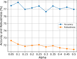
(a) Effectiveness of trained GCN

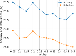
(b) Effectiveness of trained GAT

(c) Effectiveness of trained GIN

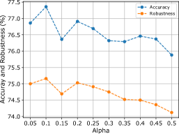
(d) Effectiveness of trained GraphSAGE

Figure 2: Accuracy and Robustness trendings with different $\alpha$.

Table 8, Table 9, Table 10, and Table 11 present the detailed results of GNN models including GCN, GAT, GraphSAGE, and GIN on the Politifact dataset when using the Mixup training strategy with different $\alpha$ settings. First, we analyze how $\alpha$ affects each type of graph pooling method. Column Std shows the standard deviation of the results of each pooling method. We can see that, in the type level, $\alpha$ also does not greatly impact the Mixup training. The maximum standard deviations are only 1.84% (Accuracy of Type 3, Table 8) and 1.73% (Robustness of Type 9, Table 10). Maybe interestingly, we can find the two most stable and least stable types, i.e., The operator Type 4 ($\mathcal{M}_{sum}(\mathcal{P}_{att},\mathcal{P}_{sum})$) from Table 8 and Type 2 ($\mathcal{M}_{mul}(\mathcal{P}_{att},\mathcal{P}_{max})$) from Table 10 always have the smallest standard deviation values for both accuracy and robustness.

Figure 2 depicts the trending of average (e.g., row Average in Table 8) results of all GNN models. Then, we can see that although both the accuracy and robustness difference between using different $\alpha$ is not that big, i.e., the gap between accuracy (robustness) is 1.30% (1.23%). The smaller $\alpha$ can produce models with better performance, which is consistent with the conclusion of the original Mixup work [8]. Especially for the robustness, there is a clear decreasing trend when $\alpha$ becomes bigger.

In conclusion, Manifold-Mixup for graph-structured data with hybrid graph pooling is resilient to the $\alpha$ setting. Moreover, small $\alpha$ is recommended in the practical usage of Mixup. Although the operator type 1 is the best for producing high-performance GNN models, Type 4 for GCN and Type 2 for GraphSAGE are the most stable method that is least affected by $\alpha$.

Answer to RQ3: The performance (both clean accuracy and robustness) of GNN models is not sensitive (with a less than 2% difference) to the change of parameter $\alpha$. A small $\alpha$ (e.g., 0.05 and o.1) is recommended for GNNs training with Manifold-Mixup.

6 Threats to Validity

The internal threat to validity comes from implementing the GNNs, each pooling method, and the Mixup for graph-structured data. The implementation of GNNs is based on [60], and the implementation of Mixup for graph data is based on the officially released project of Mixup [8].

External validity threats lie in the selected NLP and PL tasks, datasets, and GNNs. We consider both the traditional NLP tasks (text level) and PL tasks (source code level) in the study and include two datasets for each task. Particularly, for the NLP task, we consider two well-studied datasets and four types of node embedding. For the PL task, we include two popular programming languages (Java and Python). For the GNN models, we consider six famous graph neural networks: GCN, GCN-Virtual, GIN, GIN-Virtual, GAT, and GraphSAGE.

The construct threats to validity mainly come from the parameters of Mixup, randomness, and evaluation measures. Mixup only contains the parameter $\alpha$ that controls the weight of mixing two input instances. We follow the recommendation of the original Mixup algorithm and investigate the impact of this parameter. Moreover, further, we explore the impact of $\alpha$ in our study. To reduce the impact of randomness, we repeat each experiment five times with different random seeds and report the average and standard deviation results. Finally, concerning the evaluation measures, we consider both the test accuracy of the original test data and the robustness of corrupted test data. The latter one is specific for evaluating the generalization ability of GNNs.

7 Conclusions

In this paper, we comprehensively investigated how the graph pooling methods impact the effectiveness of Mixups when dealing with graph-structured data. We considered the Max-pooling operator, the state-of-the-art GMT pooling operator, and nine different hybrid pooling methods defined ourselves. In the empirical analysis part, we conducted experiments on both traditional NLP tasks (fake news detection) and PL tasks (problem classification) using six types of GNN architecture. The experimental results demonstrated that the pooling operator significantly impacts the effectiveness of Mixup, where hybrid pooling operators outperform both the Max-pooling and GMT operators in terms of producing accurate and robust GNN models. The hyperparameter $\alpha$ has a limited impact on Mixup in augmenting graph-structured data. This study gave the lesson that, when using Mixup in GNNs, carefully choosing the pooling operators could help produce better models.

References

-
[1]
L. Huang, D. Ma, S. Li, X. Zhang, H. Wang,
Text level graph neural network for
text classification, in: Proceedings of the 2019 Conference on Empirical
Methods in Natural Language Processing and the 9th International Joint
Conference on Natural Language Processing (EMNLP-IJCNLP), Association for
Computational Linguistics, Hong Kong, China, 2019, pp. 3444–3450.
doi:10.18653/v1/D19-1345.
URL https://aclanthology.org/D19-1345 - [2] M. Allamanis, E. T. Barr, P. Devanbu, C. Sutton, A survey of machine learning for big code and naturalness, ACM Computing Surveys (CSUR) 51 (4) (2018) 81.
- [3] Z. Wu, S. Pan, F. Chen, G. Long, C. Zhang, P. S. Yu, A comprehensive survey on graph neural networks, IEEE Transactions on Neural Networks and Learning Systems 32 (1) (2021) 4–24. doi:10.1109/TNNLS.2020.2978386.
- [4] E. Dinella, H. Dai, Z. Li, M. Naik, L. Song, K. Wang, Hoppity: Learning graph transformations to detect and fix bugs in programs, in: International Conference on Learning Representations (ICLR), 2020.
- [5] W. Wang, G. Li, B. Ma, X. Xia, Z. Jin, Detecting code clones with graph neural network and flow-augmented abstract syntax tree, in: 2020 IEEE 27th International Conference on Software Analysis, Evolution and Reengineering (SANER), 2020, pp. 261–271. doi:10.1109/SANER48275.2020.9054857.
-
[6]
M. Allamanis, M. Brockschmidt, M. Khademi,
Learning to represent
programs with graphs, in: International Conference on Learning
Representations, 2018.
URL https://openreview.net/forum?id=BJOFETxR- - [7] Y. Zhou, S. Liu, J. Siow, X. Du, Y. Liu, Devign: Effective Vulnerability Identification by Learning Comprehensive Program Semantics via Graph Neural Networks, Curran Associates Inc., Red Hook, NY, USA, 2019.
-
[8]
H. Zhang, M. Cisse, Y. N. Dauphin, D. Lopez-Paz,
mixup: Beyond empirical risk
minimization, in: International Conference on Learning Representations,
2018.
URL https://openreview.net/forum?id=r1Ddp1-Rb - [9] Y. Wang, W. Wang, Y. Liang, Y. Cai, B. Hooi, Mixup for node and graph classification, in: Proceedings of the Web Conference 2021, 2021, pp. 3663–3674.
- [10] Z. Dong, Q. Hu, Y. Guo, M. Cordy, M. Papadakis, Z. Zhang, Y. L. Traon, J. Zhao, Mixcode: Enhancing code classification by mixup-based data augmentation, in: 2023 IEEE International Conference on Software Analysis, Evolution and Reengineering (SANER), 2023, pp. 379–390. doi:10.1109/SANER56733.2023.00043.
-
[11]
V. Verma, A. Lamb, C. Beckham, A. Najafi, I. Mitliagkas, D. Lopez-Paz,
Y. Bengio, Manifold
mixup: Better representations by interpolating hidden states, in:
K. Chaudhuri, R. Salakhutdinov (Eds.), Proceedings of the 36th International
Conference on Machine Learning, Vol. 97 of Proceedings of Machine Learning
Research, PMLR, 2019, pp. 6438–6447.
URL https://proceedings.mlr.press/v97/verma19a.html -
[12]
L. Zhang, Z. Deng, K. Kawaguchi, J. Zou,
When and how mixup
improves calibration, in: K. Chaudhuri, S. Jegelka, L. Song, C. Szepesvari,
G. Niu, S. Sabato (Eds.), Proceedings of the 39th International Conference on
Machine Learning, Vol. 162 of Proceedings of Machine Learning Research, PMLR,
2022, pp. 26135–26160.
URL https://proceedings.mlr.press/v162/zhang22f.html -
[13]
L. Zhang, Z. Deng, K. Kawaguchi, A. Ghorbani, J. Zou,
How does mixup help with
robustness and generalization?, in: International Conference on Learning
Representations, 2021.
URL https://openreview.net/forum?id=8yKEo06dKNo - [14] B. Knyazev, G. W. Taylor, M. R. Amer, Understanding Attention and Generalization in Graph Neural Networks, Curran Associates Inc., Red Hook, NY, USA, 2019.
- [15] D. Mesquita, A. H. Souza, S. Kaski, Rethinking pooling in graph neural networks, in: Proceedings of the 34th International Conference on Neural Information Processing Systems, NIPS’20, Curran Associates Inc., Red Hook, NY, USA, 2020.
- [16] D. Grattarola, D. Zambon, F. M. Bianchi, C. Alippi, Understanding pooling in graph neural networks, IEEE Transactions on Neural Networks and Learning Systems (2022) 1–11doi:10.1109/TNNLS.2022.3190922.
-
[17]
J. Baek, M. Kang, S. J. Hwang,
Accurate learning of graph
representations with graph multiset pooling, in: International Conference on
Learning Representations, 2021.
URL https://openreview.net/forum?id=JHcqXGaqiGn - [18] V.-A. Nguyen, V. Nguyen, T. Le, Q. H. Tran, D. Phung, et al., Regvd: Revisiting graph neural networks for vulnerability detection, in: 2022 IEEE/ACM 44th International Conference on Software Engineering: Companion Proceedings (ICSE-Companion), IEEE, 2022, pp. 178–182.
- [19] L. Yao, C. Mao, Y. Luo, Graph convolutional networks for text classification, in: Proceedings of the AAAI conference on artificial intelligence, Vol. 33, 2019, pp. 7370–7377.
-
[20]
Y. Zhang, X. Yu, Z. Cui, S. Wu, Z. Wen, L. Wang,
Every document owns its
structure: Inductive text classification via graph neural networks, in:
Proceedings of the 58th Annual Meeting of the Association for Computational
Linguistics, Association for Computational Linguistics, Online, 2020, pp.
334–339.
doi:10.18653/v1/2020.acl-main.31.
URL https://aclanthology.org/2020.acl-main.31 - [21] Z. Dong, Q. Hu, Y. Guo, Z. Zhang, M. Cordy, M. Papadakis, Y. L. Traon, J. Zhao, Boosting source code learning with data augmentation: An empirical study, arXiv preprint arXiv:2303.06808.
- [22] M. Allamanis, H. Jackson-Flux, M. Brockschmidt, Self-supervised bug detection and repair, Advances in Neural Information Processing Systems 34 (2021) 27865–27876.
- [23] Z. Ying, J. You, C. Morris, X. Ren, W. Hamilton, J. Leskovec, Hierarchical graph representation learning with differentiable pooling, Advances in neural information processing systems 31.
- [24] J. Atwood, D. Towsley, Diffusion-convolutional neural networks, in: Proceedings of the 30th International Conference on Neural Information Processing Systems, NIPS’16, Curran Associates Inc., Red Hook, NY, USA, 2016, p. 2001–2009.
- [25] M. Simonovsky, N. Komodakis, Dynamic edge-conditioned filters in convolutional neural networks on graphs, in: Proceedings of the IEEE conference on computer vision and pattern recognition, 2017, pp. 3693–3702.
-
[26]
K. Xu, W. Hu, J. Leskovec, S. Jegelka,
How powerful are graph
neural networks?, in: International Conference on Learning Representations,
2019.
URL https://openreview.net/forum?id=ryGs6iA5Km - [27] M. Zhang, Z. Cui, M. Neumann, Y. Chen, An end-to-end deep learning architecture for graph classification, in: Proceedings of the AAAI conference on artificial intelligence, Vol. 32, 2018.
- [28] H. Gao, S. Ji, Graph u-nets, in: international conference on machine learning, PMLR, 2019, pp. 2083–2092.
- [29] J. Lee, I. Lee, J. Kang, Self-attention graph pooling, in: International conference on machine learning, PMLR, 2019, pp. 3734–3743.
- [30] C. Cangea, P. Veličković, N. Jovanović, T. Kipf, P. Liò, Towards sparse hierarchical graph classifiers, arXiv preprint arXiv:1811.01287.
- [31] Y. Ma, S. Wang, C. C. Aggarwal, J. Tang, Graph convolutional networks with eigenpooling, in: Proceedings of the 25th ACM SIGKDD international conference on knowledge discovery & data mining, 2019, pp. 723–731.
- [32] Y. G. Wang, M. Li, Z. Ma, G. Montúfar, X. Zhuang, Y. Fan, Haarpooling: Graph pooling with compressive haar basis.
- [33] F. M. Bianchi, D. Grattarola, C. Alippi, Spectral clustering with graph neural networks for graph pooling, in: International Conference on Machine Learning, PMLR, 2020, pp. 874–883.
- [34] H. Yuan, S. Ji, Structpool: Structured graph pooling via conditional random fields, in: Proceedings of the 8th International Conference on Learning Representations, 2020.
- [35] E. Ranjan, S. Sanyal, P. Talukdar, Asap: Adaptive structure aware pooling for learning hierarchical graph representations, in: Proceedings of the AAAI Conference on Artificial Intelligence, Vol. 34, 2020, pp. 5470–5477.
-
[36]
Y. Li, D. Tarlow, M. Brockschmidt, R. S. Zemel,
Gated graph sequence neural networks,
in: Y. Bengio, Y. LeCun (Eds.), 4th International Conference on Learning
Representations, ICLR 2016, San Juan, Puerto Rico, May 2-4, 2016,
Conference Track Proceedings, 2016.
URL http://arxiv.org/abs/1511.05493 - [37] J. Li, Y. Rong, H. Cheng, H. Meng, W. Huang, J. Huang, Semi-supervised graph classification: A hierarchical graph perspective, in: The World Wide Web Conference, 2019, pp. 972–982.
- [38] D. Bahdanau, K. Cho, Y. Bengio, Neural machine translation by jointly learning to align and translate, arXiv preprint arXiv:1409.0473.
- [39] C. Shorten, T. M. Khoshgoftaar, A survey on image data augmentation for deep learning, Journal of big data 6 (1) (2019) 1–48.
- [40] H. Guo, Y. Mao, R. Zhang, Augmenting data with mixup for sentence classification: An empirical study, arXiv preprint arXiv:1905.08941.
-
[41]
L. Sun, C. Xia, W. Yin, T. Liang, P. Yu, L. He,
Mixup-transformer:
Dynamic data augmentation for NLP tasks, in: Proceedings of the 28th
International Conference on Computational Linguistics, International
Committee on Computational Linguistics, Barcelona, Spain (Online), 2020, pp.
3436–3440.
doi:10.18653/v1/2020.coling-main.305.
URL https://aclanthology.org/2020.coling-main.305 -
[42]
J. Chen, Z. Yang, D. Yang,
MixText:
Linguistically-informed interpolation of hidden space for semi-supervised
text classification, in: Proceedings of the 58th Annual Meeting of the
Association for Computational Linguistics, Association for Computational
Linguistics, Online, 2020, pp. 2147–2157.
doi:10.18653/v1/2020.acl-main.194.
URL https://aclanthology.org/2020.acl-main.194 -
[43]
R. Zhang, Y. Yu, C. Zhang,
SeqMix: Augmenting
active sequence labeling via sequence mixup, in: Proceedings of the 2020
Conference on Empirical Methods in Natural Language Processing (EMNLP),
Association for Computational Linguistics, Online, 2020, pp. 8566–8579.
doi:10.18653/v1/2020.emnlp-main.691.
URL https://aclanthology.org/2020.emnlp-main.691 -
[44]
S. Yoon, G. Kim, K. Park,
SSMix: Saliency-based
span mixup for text classification, in: Findings of the Association for
Computational Linguistics: ACL-IJCNLP 2021, Association for Computational
Linguistics, Online, 2021, pp. 3225–3234.
doi:10.18653/v1/2021.findings-acl.285.
URL https://aclanthology.org/2021.findings-acl.285 -
[45]
R. Konno, Y. Matsubayashi, S. Kiyono, H. Ouchi, R. Takahashi, K. Inui,
An empirical study of
contextual data augmentation for Japanese zero anaphora resolution, in:
Proceedings of the 28th International Conference on Computational
Linguistics, International Committee on Computational Linguistics, Barcelona,
Spain (Online), 2020, pp. 4956–4968.
doi:10.18653/v1/2020.coling-main.435.
URL https://aclanthology.org/2020.coling-main.435 - [46] J. Chen, D. Tam, C. Raffel, M. Bansal, D. Yang, An empirical survey of data augmentation for limited data learning in nlp, Transactions of the Association for Computational Linguistics 11 (2023) 191–211.
-
[47]
S. Yu, T. Wang, J. Wang,
Data
augmentation by program transformation, Journal of Systems and Software 190
(2022) 111304.
doi:https://doi.org/10.1016/j.jss.2022.111304.
URL https://www.sciencedirect.com/science/article/pii/S0164121222000541 -
[48]
J. Gilmer, S. S. Schoenholz, P. F. Riley, O. Vinyals, G. E. Dahl,
Neural message
passing for quantum chemistry, in: D. Precup, Y. W. Teh (Eds.), Proceedings
of the 34th International Conference on Machine Learning, Vol. 70 of
Proceedings of Machine Learning Research, PMLR, 2017, pp. 1263–1272.
URL https://proceedings.mlr.press/v70/gilmer17a.html - [49] H. Xu, S. Mannor, Robustness and generalization, Machine learning 86 (3) (2012) 391–423. doi:10.1007/s10994-011-5268-1.
- [50] Y. Tu, How robust is the internet?, Nature 406 (6794) (2000) 353–354.
- [51] B. Neyshabur, S. Bhojanapalli, D. McAllester, N. Srebro, Exploring generalization in deep learning, Advances in neural information processing systems 30.
- [52] P. A. Papp, K. Martinkus, L. Faber, R. Wattenhofer, Dropgnn: Random dropouts increase the expressiveness of graph neural networks, Advances in Neural Information Processing Systems 34 (2021) 21997–22009.
-
[53]
B. Fabian, A. Baumann, J. Lackner,
Topological analysis of
cloud service connectivity, Comput. Ind. Eng. 88 (C) (2015) 151–165.
doi:10.1016/j.cie.2015.06.009.
URL https://doi.org/10.1016/j.cie.2015.06.009 -
[54]
M. Oehlers, B. Fabian, Graph
metrics for network robustness—a survey, Mathematics 9 (8).
doi:10.3390/math9080895.
URL https://www.mdpi.com/2227-7390/9/8/895 -
[55]
Y. Dou, K. Shu, C. Xia, P. S. Yu, L. Sun,
User preference-aware fake
news detection, in: Proceedings of the 44th International ACM SIGIR
Conference on Research and Development in Information Retrieval, SIGIR ’21,
Association for Computing Machinery, New York, NY, USA, 2021, p. 2051–2055.
doi:10.1145/3404835.3462990.
URL https://doi.org/10.1145/3404835.3462990 - [56] R. Puri, D. S. Kung, G. Janssen, W. Zhang, G. Domeniconi, V. Zolotov, J. Dolby, J. Chen, M. Choudhury, L. Decker, et al., Codenet: A large-scale ai for code dataset for learning a diversity of coding tasks, arXiv preprint arXiv:2105.12655.
-
[57]
T. N. Kipf, M. Welling,
Semi-supervised
classification with graph convolutional networks, in: International
Conference on Learning Representations, 2017.
URL https://openreview.net/forum?id=SJU4ayYgl - [58] P. Velickovic, G. Cucurull, A. Casanova, A. Romero, P. Lio, Y. Bengio, Graph attention networks, stat 1050 (2017) 20.
- [59] W. Hamilton, Z. Ying, J. Leskovec, Inductive representation learning on large graphs, Advances in neural information processing systems 30.
- [60] M. Fey, J. E. Lenssen, Fast graph representation learning with PyTorch Geometric, in: ICLR Workshop on Representation Learning on Graphs and Manifolds, 2019.
- [61] D. P. Kingma, J. Ba, Adam: A method for stochastic optimization, arXiv preprint arXiv:1412.6980.
- [62] S. Yun, D. Han, S. J. Oh, S. Chun, J. Choe, Y. Yoo, Cutmix: Regularization strategy to train strong classifiers with localizable features, in: Proceedings of the IEEE/CVF international conference on computer vision, 2019, pp. 6023–6032.