Distributionally Adaptive Meta Reinforcement Learning

Abstract

Meta-reinforcement learning algorithms provide a data-driven way to acquire policies that quickly adapt to many tasks with varying rewards or dynamics functions. However, learned meta-policies are often effective only on the exact task distribution on which they were trained and struggle in the presence of distribution shift of test-time rewards or transition dynamics. In this work, we develop a framework for meta-RL algorithms that are able to behave appropriately under test-time distribution shifts in the space of tasks. Our framework centers on an adaptive approach to distributional robustness that trains a population of meta-policies to be robust to varying levels of distribution shift. When evaluated on a potentially shifted test-time distribution of tasks, this allows us to choose the meta-policy with the most appropriate level of robustness, and use it to perform fast adaptation. We formally show how our framework allows for improved regret under distribution shift, and empirically show its efficacy on simulated robotics problems under a wide range of distribution shifts.

1 Introduction

The diversity and dynamism of the real world require reinforcement learning (RL) agents that can quickly adapt and learn new behaviors when placed in novel situations. Meta reinforcement learning provides a framework for conferring this ability to RL agents, by learning a “meta-policy” trained to adapt as quickly as possible to tasks from a provided training distribution [39, 10, 33, 48]. Unfortunately, meta-RL agents assume tasks to be always drawn from the training task distribution and often behave erratically when asked to adapt to tasks beyond the training distribution [5, 8]. As an example of this negative transfer, consider using meta-learning to teach a robot to navigate to goals quickly (illustrated in Figure 1). The resulting meta-policy learns to quickly adapt and walk to any target location specified in the training distribution, but explores poorly and fails to adapt to any location not in that distribution. This is particularly problematic for the meta-learning setting, since the scenarios where we need the ability to learn quickly are usually exactly those where the agent experiences distribution shift. This type of meta-distribution shift afflicts a number of real-world problems including autonomous vehicle driving [9], in-hand manipulation [17, 1], and quadruped locomotion [24, 22, 18], where training task distribution may not encompass all real-world scenarios.

In this work, we study meta-RL algorithms that learn meta-policies resilient to task distribution shift at test time. We assume the test-time distribution shift to be unknown but fixed. One approach to enable this resiliency is to leverage the framework of distributional robustness [37], training meta-policies that prepare for distribution shifts by optimizing the worst-case empirical risk against a set of task distributions which lie within a bounded distance from the original training task distribution (often referred to as an uncertainty set)). This allows meta-policies to deal with potential test-time task distribution shift, bounding their worst-case test-time regret for distributional shifts within the chosen uncertainty set. However, choosing an appropriate uncertainty set can be quite challenging without further information about the test environment, significantly impacting the test-time performance of algorithms under distribution shift. Large uncertainty sets allow resiliency to a wider range of distribution shifts, but the resulting meta-policy adapts very slowly at test time; smaller uncertainty sets enable faster test-time adaptation, but leave the meta-policy brittle to task distribution shifts. Can we get the best of both worlds?

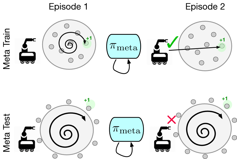
Figure 1: Failure of Typical Meta-RL. On meta-training tasks, $\pi_{\text{meta}}$ explores effectively and quickly learns the optimal behavior (top row). When test tasks come from a slightly larger task distribution, exploration fails catastrophically, resulting in poor adaptation behavior (bottom row).

Our key insight is that we can prepare for a variety of potential test-time distribution shifts by constructing and training against different uncertainty sets at training time. By preparing for adaptation against each of these uncertainty sets, an agent is able to adapt to a variety of potential test-time distribution shifts by adaptively choosing the most appropriate level of distributional robustness for the test distribution at hand. We introduce a conceptual framework called distributionally adaptive meta reinforcement learning, formalizing this idea. At train time, the agent learns robust meta-policies with widening uncertainty sets, preemptively accounting for different levels of test-time distribution shift that may be encountered. At test time, the agent infers the level of distribution shift it is faced with, and then uses the corresponding meta-policy to adapt to the new task (Figure 2). In doing so, the agent can adaptively choose the best level of robustness for the test-time task distribution, preserving the fast adaptation benefits of meta RL, while also ensuring good asymptotic performance under distribution shift. We instantiate a practical algorithm in this framework (DiAMetR), using learned generative models to imagine new task distributions close to the provided training tasks that can be used to train robust meta-policies.

The contribution of this paper is to propose a framework for making meta-reinforcement learning resilient to a variety of task distribution shifts, and DiAMetR, a practical algorithm instantiating the framework. DiAMetR trains a population of meta-policies to be robust to different degrees of distribution shifts and then adaptively chooses a meta-policy to deploy based on the inferred test-time distribution shift. Our experiments verify the utility of adaptive distributional robustness under test-time task distribution shift in a number of simulated robotics domains.

2 Related Work

Meta-reinforcement learning algorithms aim to leverage a distribution of training tasks to “learn a reinforcement learning algorithm", that is able to learn as quickly on new tasks drawn from the same distribution. A variety of algorithms have been proposed for meta-RL, including memory-based  [7, 25], gradient-based [10, 35, 13] and latent-variable based [33, 48, 47, 11] schemes. These algorithms show the ability to generalize to new tasks drawn from the same distribution, and have been applied to problems ranging from robotics [27, 47, 18] to computer science education [43]. This line of work has been extended to operate in scenarios without requiring any pre-specified task distribution  [12, 16], in offline settings  [6, 28, 26] or in hard (meta-)exploration settings [49, 46], making them more broadly applicable to a wider class of problems. However, most meta-RL algorithms assume source and target tasks are drawn from the same distribution, an assumption rarely met in practice. Our work shows how the machinery of meta-RL can be made compatible with distribution shift at test time, using ideas from distributional robustness. Some recent work shows that model based meta-reinforcement learning can be made to be robust to a particular level distribution shift  [23, 20] by learning a shared dynamics model against adversarially chosen task distributions. We show that we can build model-free meta-reinforcement learning algorithms, which are not just robust to a particular level of distribution shift, but can adapt to various levels of shift.

Distributional robustness methods have been studied in the context of building supervised learning systems that are robust to the test distribution being different than the training one. The key idea is to train a model to not just minimize empirical risk, but instead learn a model that has the lowest worst-case empirical risk among an “uncertainty-set" of distributions that are boundedly close to the empirical training distribution [37, 21, 2, 15]. If the uncertainty set and optimization are chosen carefully, these methods have been shown to obtain models that are robust to small amounts of distribution shift at test time [37, 21, 2, 15], finding applications in problems like federated learning [15] and image classification [21]. This has been extended to the min-max robustness setting for specific algorithms like model-agnostic meta-learning  [3], but are critically dependent on correct specification of the appropriate uncertainty set and applicable primarily in supervised learning settings. Alternatively, several RL techniques aim to directly tackle the robustness problem, aiming to learn policies robust to adversarial perturbations [41, 45, 32, 31]. [44] conditions the policy on uncertainty sets to make it robust to different perturbation sets. While these methods are able to learn conservative, robust policies, they are unable to adapt to new tasks as DiAMetR does in the meta-reinforcement learning setting. In our work, rather than choosing a single uncertainty set, we learn many meta-policies for widening uncertainty sets, thereby accounting for different levels of test-time distribution shift.

3 Preliminaries

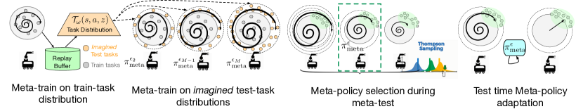
Figure 2: During meta-train, DiAMetR learns a meta-policy $\pi_{\text{meta}}^{\epsilon_{1}}$ and task distribution model ${\mathcal{T}}_{\omega}(s,a,z)$ on train task distribution. Then, it uses the task distribution model to imagine different shifted test task distributions on which it learns different meta-policies $\{\pi_{\text{meta}}^{\epsilon_{i}}\}_{i=2}^{M}$, each corresponding to a different level of robustness. During meta-test, it chooses an appropriate meta-policy based on inferred test task distribution shift with Thompson’s sampling and then quickly adapts the selected meta-policy to individual tasks.

Meta-Reinforcement Learning aims to learn a fast reinforcement learning algorithm or a “meta-policy" that can quickly maximize performance on tasks ${\mathcal{T}}$ from some distribution $p(\mathcal{T})$. Formally, each task ${\mathcal{T}}$ is a Markov decision process (MDP) $\mathcal{M}=(\mathcal{S},\mathcal{A},\mathcal{P},\mathcal{R},\gamma,\mu_{0})$; the goal is to exploit regularities in the structure of rewards and environment dynamics across tasks in $p({\mathcal{T}})$ to acquire effective exploration and adaptation mechanisms that enable learning on new tasks much faster than learning the task naively from scratch. A meta-policy (or fast learning algorithm) $\pi_{\text{meta}}$ maps a history of environment experience $h\in({\mathcal{S}}\times{\mathcal{A}}\times{\mathcal{R}})^{*}$ in a new task to an action $a$, and is trained to acquire optimal behaviors on tasks from $p({\mathcal{T}})$ within $k$ episodes:

$$\min_{\pi_{\text{meta}}}\mathbb{E}_{{\mathcal{T}}\sim p({\mathcal{T}})}\left[\operatorname{Regret}(\pi_{\text{meta}},{\mathcal{T}})\right],$$

$$\operatorname{Regret}(\pi_{\text{meta}},{\mathcal{T}}) =J(\pi_{\mathcal{T}}^{*})-\mathbb{E}_{a_{t}^{(i)}\sim\pi_{\text{meta}}(\cdot|h_{t}^{(i)}),{\mathcal{T}}}\left[\frac{1}{k}\sum_{i=1}^{k}\sum_{t=1}^{T}r_{t}^{(i)}\right],\;\;J(\pi_{\mathcal{T}}^{*})=\max_{\pi}\mathbb{E}_{\pi,{\mathcal{T}}}[\sum_{t}r_{t}]$$

where $$h_{t}^{(i)}=(s_{1:t}^{(i)},r_{1:t}^{(i)},a_{1:t-1}^{(i)})\cup(s_{1:T}^{(j)},r_{1:T}^{(j)},a_{1:T}^{(j)})_{j=1}^{i-1}.$$ (1)

Intuitively, the meta-policy has two components: an exploration mechanism that ensures that appropriate reward signal is found for all tasks in the training distribution, and an adaptation mechanism that uses the collected exploratory data to generate optimal actions for the current task. In practice, the meta-policy may be represented explicitly as an exploration policy conjoined with a policy update[10, 33], or implicitly as a black-box RNN [7, 48]. We use the terminology “meta-policies" interchangeably with that of “fast-adaptation" algorithms, since our practical implementation builds on  [30] (which represents the adaptation mechanism using a black-box RNN). Our work focuses on the setting where there is potential drift between $p_{\text{train}}({\mathcal{T}}$), the task distribution we have access to during training, and $p_{\text{test}}({\mathcal{T}})$, the task distribution of interest during evaluation.

Distributional robustness  [37] learns models that do not minimize empirical risk against the training distribution, but instead prepare for distribution shift by optimizing the worst-case empirical risk against a set of data distributions close to the training distribution (called an uncertainty set):

$$\min_{\theta} ~{}\max_{\phi}\mathbb{E}_{x\sim q_{\phi}(x)}[l(x;\theta)]~{}~{}~{}~{}~{}~{}\text{s.t.}~{}~{}~{}D(p_{\text{train}}(x)||q_{\phi}(x))\leq\epsilon$$ (2)

This optimization finds the model parameters $\theta$ that minimizes worst case risk $l$ over distributions $q_{\phi}(x)$ in an $\epsilon$-ball (measured by an $f$-divergence) from the training distribution $p_{\text{train}}(x)$.

4 Distributionally Adaptive Meta-Reinforcement Learning

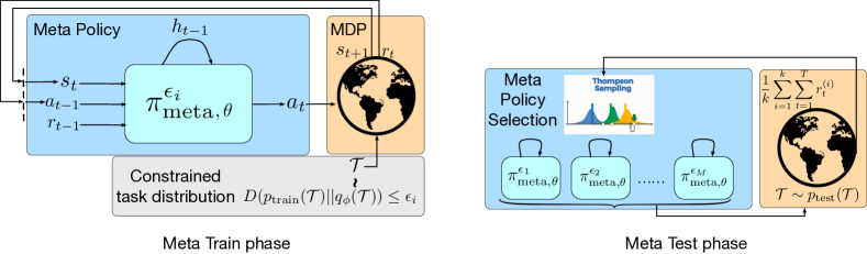
Figure 3: During meta-train phase, DiAMetR learns a family of meta-policies robust to varying levels of distribution shift (as characterized by $\epsilon_{i}$). During meta-test phase, given a potentially shifted test-time distribution of tasks, DiAMetR chooses the meta-policy with the most appropriate level of robustness and use it to perform fast adaptation for new tasks sampled from the same shifted test task distribution.

In this section, we develop a framework for learning meta-policies, that given access to a training distribution of tasks $p_{\text{train}}(\mathcal{T})$, is still able to adapt to tasks from a test-time distribution $p_{\text{test}}(\mathcal{T})$ that is similar but not identical to the training distribution. We introduce a framework for distributionally adaptive meta-RL below and instantiate it as a practical method in Section 5.

4.1 Known Level of Test-Time Distribution Shift

We begin by studying a simplified problem where we can exactly quantify the degree to which the test distribution deviates from the training distribution. Suppose we know that $p_{\text{test}}$ satisfies $D(p_{\text{test}}({\mathcal{T}})||p_{\text{train}}({\mathcal{T}}))<\epsilon$ for some $\epsilon>0$, where $D(\cdot\|\cdot)$ is a probability divergence on the set of task distributions (e.g. an $f$-divergence [34] or a Wasserstein distance [40]). A natural learning objective to learn a meta-policy under this assumption is to minimize the worst-case test-time regret across any test task distribution $q({\mathcal{T}})$ that is within some $\epsilon$ divergence of the train distribution:

$$\min_{\pi_{\text{meta}}}~{} {\mathcal{R}}(\pi_{\text{meta}},p_{\text{train}}({\mathcal{T}}),\epsilon),$$

$${\mathcal{R}}(\pi_{\text{meta}},p_{\text{train}}({\mathcal{T}}),\epsilon) =\max_{q({\mathcal{T}})}\mathbb{E}_{{\mathcal{T}}\sim q({\mathcal{T}})}\left[\operatorname{Regret}(\pi_{\text{meta}},{\mathcal{T}})\right]~{}~{}~{}~{}~{}~{}\text{s.t.}~{}~{}D(p_{\text{train}}({\mathcal{T}})\|q({\mathcal{T}}))\leq\epsilon$$ (3)

Solving this optimization problem results in a meta-policy that has been trained to adapt to tasks from a wider task distribution than the original training distribution. It is worthwhile distinguishing this robust meta-objective, which incentivizes a robust adaptation mechanism to a wider set of tasks, from robust objectives in standard RL, which produce base policies robust to a wider set of dynamics conditions. The objective in Eq 3 incentivizes an agent to explore and adapt more broadly, not act more conservatively as standard robust RL methods  [32] would encourage. Naturally, the quality of the robust meta-policy depends on the size of the uncertainty set. If $\epsilon$ is large, or the geometry of the divergence poorly reflect natural task variations, then the robust policy will have to adapt to an overly large set of tasks, potentially degrading the speed of adaptation.

4.2 Handling Arbitrary Levels of Distribution Shift

In practice, it is not known how the test distribution $p_{\text{test}}$ deviates from the training distribution, and consequently it is challenging to determine what $\epsilon$ to use in the meta-robustness objective. We propose to overcome this via an adaptive strategy: to train meta-policies for varying degrees of distribution shift, and at test-time, inferring which distribution shift is most appropriate through experience.

We train a population of meta-policies $\{\pi_{\text{meta}}^{(i)}\}_{i=1}^{M}$, each solving the distributionally robust meta-RL objective (eq 3) for a different level of robustness $\epsilon_{i}$:

$$\left\{\pi_{\text{meta}}^{\epsilon_{i}}\coloneqq\arg\min_{\pi_{\text{meta}}}{\mathcal{R}}(\pi_{\text{meta}},p_{\text{train}}({\mathcal{T}}),\epsilon_{i})\right\}_{i=1}^{M}~{}~{}~{}\text{ where }\epsilon_{M}>\epsilon_{M-1}>\ldots>\epsilon_{1}=0$$ (4)

In choosing a spectrum of $\epsilon_{i}$, we learn a set of meta-policies that have been trained on increasingly large set of tasks: at one end ($i=1$), the meta-policy is trained only on the original training distribution, and at the other ($i=M$), the meta-policy trained to adapt to any possible task within the parametric family of tasks. These policies span a tradeoff between being robust to a wider set of task distributions with larger $\epsilon$ (allowing for larger distribution shifts), and being able to adapt quickly to any given task with smaller $\epsilon$ (allowing for better per-task regret minimization).

With a set of meta-policies in hand, we must now decide how to leverage test-time experience to discover the right one to use for the actual test distribution $p_{\text{test}}$. We recognize that the problem of policy selection can be treated as a stochastic multi-armed bandit problem (precise formulation in Appendix C), where pulling arm $i$ corresponds to running the meta-policy $\pi_{\text{meta}}^{\epsilon_{i}}$ for an entire meta-episode ($k$ task episodes). If a zero-regret bandit algorithm (eg: Thompson’s sampling [42]) is used , then after a certain number of test-time meta episodes, we can guarantee that the meta-policy selection mechanism will converge to the meta-policy that best balances the tradeoff between adapting quickly while still being able to adapt to all the tasks from $p_{\text{test}}({\mathcal{T}})$.

To summarize our framework for distributionally adaptive meta-RL, we train a population of meta-policies at varying levels of robustness on a distributionally robust objective that forces the learned adaptation mechanism to also be robust to tasks not in the training task distribution. At test-time, we use a bandit algorithm to select the meta-policy whose adaptation mechanism has the best tradeoff between robustness and speed of adaptation specifically on the test task distribution. Combining distributional robustness with test-time adaptation allows the adaptation mechanism to work even if distribution shift is present, while obviating the decreased performance that usually accompanies overly conservative, distributionally robust solutions.

4.3 Analysis

To provide some intuition on the properties of this algorithm, we formally analyze adaptive distributional robustness in a simplified meta RL problem involving tasks ${\mathcal{T}}_{g}$ corresponding to reaching some unknown goal $g$ in a deterministic MDP ${\mathcal{M}}$, exactly at the final timestep of an episode. We assume that all goals are reachable, and use the family of meta-policies that use a stochastic exploratory policy $\pi$ until the goal is discovered and return to the discovered goal in all future episodes. The performance of a meta-policy on a task ${\mathcal{T}}_{g}$ under this model can be expressed in terms of the state distribution of the exploratory policy: $\operatorname{Regret}(\pi_{\text{meta}},{\mathcal{T}}_{g})=\frac{1}{d_{\pi}^{T}(g)}$. This particular framework has been studied in  [12, 19], and is a simple, interpretable framework for analysis.

We seek to understand performance under distribution shift when the original training task distribution is relatively concentrated on a subset of possible tasks. We choose the training distribution $p_{\text{train}}({\mathcal{T}}_{g})=(1-\beta)\text{Uniform}({\mathcal{S}}_{0})+\beta\text{Uniform}({\mathcal{S}}\backslash{\mathcal{S}}_{0})$, so that $p_{\text{train}}$ is concentrated on tasks involving a subset of the state space ${\mathcal{S}}_{0}\subset{\mathcal{S}}$, with $\beta$ a parameter dictating the level of concentration, and consider test distributions that perturb under the TV metric. Our main result compares the performance of a meta-policy trained to an $\epsilon_{2}$-level of robustness when the true test distribution deviates by $\epsilon_{1}$.

Proposition 4.1.

Let $\overline{\epsilon_{i}}=\min\{\epsilon_{i}+\beta,1-\frac{|{\mathcal{S}}_{0}|}{|{\mathcal{S}}|}\}$. There exists $q({\mathcal{T}})$ satisfying $D_{TV}(p_{\text{train}},q)\leq\epsilon_{1}$ where an $\epsilon_{2}$-robust meta policy incurs excess regret over the optimal $\epsilon_{1}$-robust meta-policy:

$$\mathbb{E}_{q({\mathcal{T}})}[\operatorname{Regret}(\pi_{\text{meta}}^{\epsilon_{2}},{\mathcal{T}})-\operatorname{Regret}(\pi_{\text{meta}}^{\epsilon_{1}},{\mathcal{T}})]\geq~{}\left(c(\epsilon_{1},\epsilon_{2})+\frac{1}{c(\epsilon_{1},\epsilon_{2})}-2\right)$$ (5)

$$~{}\sqrt{\overline{\epsilon_{1}}(1-\overline{\epsilon_{1}})|{\mathcal{S}}_{0}|(|{\mathcal{S}}|-{\mathcal{S}}_{0}|)}$$ (6)

The scale of regret depends on $c(\epsilon_{1},\epsilon_{2})=\sqrt{\tfrac{\overline{\epsilon_{2}}^{-1}-1}{\overline{\epsilon_{1}}^{-1}-1}}$, a measure of the mismatch between $\epsilon_{1}$ and $\epsilon_{2}$.

We first compare robust and non-robust solutions by analyzing the bound when $\epsilon_{2}=0$. In the regime of $\beta\ll 1$, excess regret scales as ${\mathcal{O}}(\epsilon_{1}\sqrt{\tfrac{1}{\beta}})$, meaning that the robust solution is most necessary when the training distribution is highly concentrated in a subset of the task space. At one extreme, if the training distribution contains no examples of tasks outside ${\mathcal{S}}_{0}$ ($\beta=0$), the non-robust solution incurs infinite excess regret; at the other extreme, if the training distribution is uniform on the set of all possible tasks ($\beta=1-\tfrac{|{\mathcal{S}}_{0}|}{|{\mathcal{S}}|}$), robustness provides no benefit.

We next quantify the effect of mis-specifying the level of robustness in the meta-robustness objective, and what benefits adaptive distributional robustness can confer. For small $\beta$ and fixed $\epsilon_{1}$, the excess regret of an $\epsilon_{2}$-robust policy scales as ${\mathcal{O}}(\sqrt{\max\{\tfrac{\epsilon_{2}}{\epsilon_{1}},\tfrac{\epsilon_{1}}{\epsilon_{2}}\}})$, meaning that excess regret gets incurred if the meta-policy is trained either to be too robust $(\epsilon_{2}\gg\epsilon_{1})$ or not robust enough $\epsilon_{1}\gg\epsilon_{2}$. Compared to a fixed robustness level, our strategy of training meta-policies for a sequence of robustness levels $\{\epsilon_{i}\}_{i=1}^{M}$ ensures that this misspecification constant is at most the relative spacing between robustness levels: $\max_{i}\frac{\epsilon_{i}}{\epsilon_{i-1}}$. This enables the distributionally adaptive approach to control the amount of excess regret by making the sequence more fine-grained, while a fixed choice of robustness incurs larger regret (as we verify empirically in our experiments as well).

Algorithm 1 DiAMetR:Meta-training phase

1:  Given: $p_{\text{train}}({\mathcal{T}})$, Return: $\{\pi_{\text{meta},\theta}^{\epsilon_{i}}\}_{i=1}^{M}$

2:  $\pi_{\text{meta},\theta}^{\epsilon_{1}}$, ${\mathcal{D}}_{\text{Replay-Buffer}}\leftarrow$ Solve equation 1 with off-policy $\text{RL}^{2}$

3:  Prior $p_{\text{train}}({\mathcal{T}})\leftarrow$ Solve eq 8 using ${\mathcal{D}}_{\text{Replay-Buffer}}$

4:  for $\epsilon$ in $\{\epsilon_{2},\ldots,\epsilon_{M}\}$ do

5:    Initialize $q_{\phi}$, $\pi_{\text{meta},\theta}^{\epsilon}$ and $\lambda\geq 0$.

6:    for iteration $n=1,2,...$ do

7:       Meta-policy: Update $\pi_{\text{meta},\theta}^{\epsilon}$ using off-policy $\text{RL}^{2}$ [30]

$$\theta\coloneqq\theta+\alpha\nabla_{\theta}\mathbb{E}_{{\mathcal{T}}\sim q_{\phi}({\mathcal{T}})}[\mathbb{E}_{\pi_{\text{meta},\theta}^{\epsilon},{\mathcal{P}}_{\mathcal{T}}}[\frac{1}{k}\sum_{i=1}^{k}\sum_{t=1}^{T}r_{\mathcal{T}}(s_{t}^{(i)},a_{t}^{(i)})]]$$

8:       Adversarial task distribution: Update $q_{\phi}$ using Reinforce [38]

$$\phi\coloneqq\phi-\alpha\nabla_{\phi}(\mathbb{E}_{{\mathcal{T}}\sim q_{\phi}({\mathcal{T}})}[\mathbb{E}_{\pi_{\text{meta},\theta}^{\epsilon},{\mathcal{P}}_{\mathcal{T}}}[\frac{1}{k}\sum_{i=1}^{k}\sum_{t=1}^{T}r_{\mathcal{T}}(s_{t}^{(i)},a_{t}^{(i)})]]+\lambda D_{\text{KL}}(p_{\text{train}}({\mathcal{T}})\|q_{\phi}({\mathcal{T}})))$$

9:       Lagrange constraint multiplier: Update $\lambda$ to enforce $D_{\text{KL}}(p_{\text{train}}\|q_{\phi})<\epsilon$,

$$\lambda\coloneqq_{\lambda\geq 0}\lambda+\alpha(D_{\text{KL}}(p_{\text{train}}({\mathcal{T}})\|q_{\phi}({\mathcal{T}}))-\epsilon)$$

10:    end for

11:  end for

5 DiAMetR: A Practical Algorithm for Meta-Distribution Shift

In order to instantiate our distributionally adaptive framework into a practical algorithm, we must address how task distributions should be parameterized and optimized over . We must also address how the robust meta-RL problem can be solved with stochastic gradient methods. We first introduce the individual components of task parameterization and robust optimization, describe the overall algorithm in Algorithm 1 and  2, and visualize components of DiAMetR in Fig 3.

5.1 Parameterizing Task Distributions

Handling in-support distribution shifts: For handling in-support task distribution shifts, we propose to represent new task distributions as re-weighted training task distribution $q({\mathcal{T}})\propto w_{\mathcal{T}}p_{\text{train}}({\mathcal{T}})$ where $w_{\mathcal{T}}>0$ is a parameter. Since we have a finite set of training tasks, say $\{{\mathcal{T}}_{i}\}_{i=1}^{n_{\text{tr}}}$, new task distributions become $q({\mathcal{T}}_{i})=\frac{w_{{\mathcal{T}}_{i}}}{\sum_{i=1}^{n_{\text{tr}}}w_{{\mathcal{T}}_{i}}}$. With a slight abuse of notation, we can write empirical training task distribution as $p_{\text{train}}({\mathcal{T}}_{i})=\frac{1}{n_{\text{tr}}}$. We can use KL divergence to measure the divergence between training task distribution and test task distribution $D(p_{\text{train}}({\mathcal{T}})\|q_{\phi}({\mathcal{T}}))=\sum_{i=1}^{n_{\text{tr}}}\frac{1}{n_{\text{tr}}}\log\frac{\sum_{i=1}^{n_{\text{tr}}}w_{{\mathcal{T}}_{i}}}{n_{\text{tr}}w_{{\mathcal{T}}_{i}}}$. We collectively represent the parameters $\phi=\{w_{{\mathcal{T}}_{i}}\}_{i=1}^{n_{\text{tr}}}$. Using this parameterization, the training objective (equation 3) becomes

$$\max_{\theta} \min_{\phi}\mathbb{E}_{{\mathcal{T}}\sim p_{\text{train}}({\mathcal{T}})}\left[\mathbb{E}_{\pi_{\text{meta},\theta}^{\epsilon},{\mathcal{P}}}\left[\frac{nw_{\mathcal{T}}}{\sum_{i=1}^{n_{\text{tr}}}w_{{\mathcal{T}}_{i}}}\frac{1}{k}\sum_{i=1}^{k}\sum_{t=1}^{T}r_{t}^{(i)}\right]\right]$$

$$~{}D_{\text{KL}}(p_{\text{train}}({\mathcal{T}})||q_{\phi}({\mathcal{T}}))\leq\epsilon$$ (7)

Handling out-of-support distribution shift: For handling out-of-support task distribution shifts, we propose to learn a probabilistic model of the training task distribution, and use the learned latent representation as a space on which to parameterize uncertainty sets over new task distributions. Specifically, we jointly train a task encoder $q_{\psi}(z|h)$ that encodes an environment history into the latent space, and a decoder ${\mathcal{T}}_{\omega}(s,a,z)$ mapping a latent vector $z$ to a property of the task using a dataset of trajectories collected from the training tasks. To describe the exact form of ${\mathcal{T}}_{\omega}$, we consider how tasks can differ and list two scenarios: (1) Tasks differ in reward functions: ${\mathcal{T}}_{\omega}$ takes form of reward functions $r_{\omega}(s,a,z)$ that maps a latent vector $z$ to a reward function and (2) Tasks differ in dynamics: ${\mathcal{T}}_{\omega}$ takes form of dynamics $p_{\omega}(s,a,z)$ that maps a latent vector $z$ to a dynamics function. This generative model can be trained as a standard latent variable model by maximizing a standard evidence lower bound (ELBO), trading off reward prediction and matching a prior $p_{\text{train}}(z)$ (chosen to be the unit gaussian).

$$\min_{\omega,\psi}\mathbb{E}_{h\sim{\mathcal{D}}}\left[\mathbb{E}_{z\sim q_{\psi}(z|h)}\left[\sum_{t=1}^{T}l({\mathcal{T}}_{\omega}(s_{t},a_{t},z),h,t)\right]+D_{\text{KL}}(q_{\psi}(z|h)||{\mathcal{N}}(0,I))\right]$$

$$l({\mathcal{T}}_{\omega}(s_{t},a_{t},z),h,t)={\color[rgb]{.75,0,.25}(r_{\omega}(s_{t},a_{t},z)-r_{t})^{2}}\;\;\;\text{{\color[rgb]{.75,0,.25}when rewards differ}}$$

$$l({\mathcal{T}}_{\omega}(s_{t},a_{t},z),h,t)={\color[rgb]{.75,.5,.25}\|p_{\omega}(s_{t},a_{t},z)-s_{t+1}\|^{2}}\;\;\;\text{{\color[rgb]{.75,.5,.25}when dynamics differ}}$$ (8)

Having learned a latent space, we can parameterize new task distributions $q({\mathcal{T}})$ as distributions $q_{\phi}(z)$ (the original training distribution corresponds to $p_{\text{train}}(z)={\mathcal{N}}(0,I)$, and measure the divergence between task distributions as well using the KL divergence in this latent space $D(p_{\text{train}}(z)\|q_{\phi}(z))$. Using this parameterization, the training objective (equation 3) becomes

$$\max_{\theta} \min_{\phi}\mathbb{E}_{z\sim q_{\phi}(z)}\left[\mathbb{E}_{\pi_{\text{meta},\theta}^{\epsilon},{\mathcal{P}}}\left[\frac{1}{k}\sum_{i=1}^{k}\sum_{t=1}^{T}{\color[rgb]{.75,0,.25}r_{\omega}(s_{t}^{(i)},a_{t}^{(i)},z)}\right]\right]\;\;\;{\color[rgb]{.75,0,.25}\text{when rewards differ}}$$

$$\max_{\theta} \min_{\phi}\mathbb{E}_{z\sim q_{\phi}(z)}\left[\mathbb{E}_{\pi_{\text{meta},\theta}^{\epsilon},{\color[rgb]{.75,.5,.25}p_{\omega}(\cdot,\cdot,z)}}\left[\frac{1}{k}\sum_{i=1}^{k}\sum_{t=1}^{T}r_{t}^{(i)}\right]\right]\;\;\;{\color[rgb]{.75,.5,.25}\text{when dynamics differ}}$$

$$~{}D_{\text{KL}}(p_{\text{train}}(z)||q_{\phi}(z))\leq\epsilon$$ (9)

5.2 Training and test-time selection of meta-policies

Learning Robust Meta-Policies: Given this task parameterization, the next question becomes how to actually perform the robust optimization laid out in Eq:3. The distributional meta-robustness objective can be modelled as an adversarial game between a meta-policy $\pi_{\text{meta}}^{\epsilon}$ and a task proposal distribution $q({\mathcal{T}})$. As described above, this task proposal distribution is parameterized as a distribution over latent space $q_{\phi}(z)$, while $\pi_{\text{meta}}^{\epsilon}$ is parameterized a typical recurrent neural network policy as in  [30]. We parameterize $\{\pi_{\text{meta}}^{\epsilon_{i}}\}_{i=1}^{M}$ as a discrete set of meta-policies, with one for each chosen value of $\epsilon$.

This leads to a simple alternating optimization scheme (see Algorithm 1), where the meta-policy is trained using a standard meta-RL algorithm (we use off-policy RL² [30] as a base learner), and the task proposal distribution with an constrained optimization method (we use dual gradient descent [29]). Each iteration $n$, three updates are performed: 1) the meta-policy $\pi_{\text{meta},\theta}$ updated to improve performance on the current task distribution, 2) the task distribution $q_{\phi}({\mathcal{T}})$ updated to increase weight on tasks where the current meta-policy adapts poorly and decreases weight on tasks that the current meta-policy can learn, while staying close to the original training distribution, and 3) a penalty coefficient $\lambda$ is updated to ensure that $q_{\phi}({\mathcal{T}})$ satisfies the divergence constraint.

Algorithm 2 DiAMetR: Meta-test phase

1:  Given: $p_{\text{test}}({\mathcal{T}})$, $\Pi=\{\pi_{\text{meta},\theta}^{\epsilon_{i}}\}_{i=1}^{M}$

2:  Initialize TS = Thompson-Sampler()

3:  for meta-episode $n=1,2,...$ do

4:    Choose meta-policy $i$ = TS.sample()

5:    Run $\pi_{\text{meta},\theta}^{\epsilon_{i}}$ for meta-episode

6:    TS.update(    arm=i,    reward=meta-episode return)

7:  end for

Test-time meta-policy selection: Since test-time meta-policy selection can be framed as a multi-armed bandit problem, we use a generic Thompson’s sampling [42] algorithm (see Algorithm 2). Each meta-episode $n$, we sample a meta-policy $\pi_{\text{meta}}^{\epsilon}$ with probability proportional to its estimated average episodic reward, run the sampled meta-policy $\pi_{\text{meta}}^{\epsilon}$ for an meta-episode ($k$ environment episodes) and then update the estimate of the average episodic reward. Since Thompson’s sampling is a zero-regret bandit algorithm, it will converge to the meta-policy that achieves the highest average episodic reward and lowest regret on the test task distribution.

6 Experimental Evaluation

(a) Ant navigation

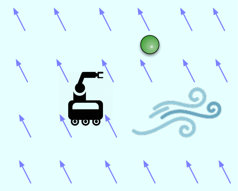
(b) Wind navigation

(c) Object localization

(d) Block push

Figure 4: The agent needs to either navigate in absence of winds, navigate in presence of winds, use its gripper to localize an object at an unobserved target location or push the block to an unobserved target location, indicated by green sphere (or cube), by exploring its environment and experiencing reward. While tasks vary in reward functions for Ant navigation, Object localization and Block push, they vary in dynamics function for Wind navigation.

We aim to comprehensively evaluate DiAMetR and answer the following questions: (1) Do meta-policies learned via DiAMetR allow for quick adaptation under different distribution shifts in the test-time task distribution? (2) Does learning for multiple levels of robustness actually help the algorithm adapt more effectively than a particular chosen uncertainty level? (3) Does proposing uncertainty sets via generative modeling provide useful distributions of tasks for robustness?

Setup. We use DiAMetR on four continuous control environments: Ant navigation (controlling a four-legged robotic quadruped), Wind navigation [6] (controlling a linear system robot in presence of wind), Object localization (controlling a Fetch robot to localize an object through its gripper) and Block push (controlling a robot arm to push an object) [13] (Figures 4(a), 4(b), 4(c) and 4(d)) (see Appendix D for details about reward function and dynamics). We design various meta RL tasks from these environments. Each meta RL task has a train task distribution $\mathcal{T}_{i}\sim p_{\text{train}}(\mathcal{T})$ such that each task $\mathcal{T}_{i}$ either parameterizes a reward function $r_{i}(s,a)\coloneqq r(s,a,\mathcal{T}_{i})$ or a dynamics function $p_{i}(s,a)\coloneqq p(s,a,\mathcal{T}_{i})$. ${\mathcal{T}}_{i}$ itself remains unobserved, the agent simply has access to reward values and executing actions in the environment. The learned meta-policies are evaluated on different distributionally shifted test task distributions $\{p^{i}_{\text{test}}(\mathcal{T})\}_{i=1}^{K}$ which are either in-support or out-of-support of training task distribution. In all meta RL tasks, the train and test task distribution is determined by the distribution of an underlying task parameter (i.e. wind velocity $w_{\mathcal{T}}$ for Wind navigation and target location $s_{\mathcal{T}}$ for other environments), which either determines the reward function or the dynamics function. While tasks vary in reward functions for Ant navigation, Object localization and Block push, they vary in dynamics function for Wind navigation (exact task distributions in Table 2). We use $4$ random seeds for all our experiments and include the standard error bars in our plots.

6.1 Adaptation to Varying Levels of Distribution Shift

During meta test, given a test task distribution $p_{\text{test}}({\mathcal{T}})$, DiAMetR uses Thompson sampling to select the appropriate meta-policy $\pi_{\text{meta},\theta}^{\epsilon}$ within $N=250$ meta episodes. $\pi_{\text{meta},\theta}^{\epsilon}$ can then solve any new task ${\mathcal{T}}\sim p_{\text{test}}({\mathcal{T}})$ within $1$ meta episode ($k$ environment episode). To test DiAMetR’s ability to adapt to varying levels of distribution shift, we evaluate it on different test task distributions, as detailed in Table 2. We compare DiAMetR with meta RL algorithms such as (off-policy) $\text{RL}^{2}$ [30], VariBAD [48] and HyperX [49]. Since DiAMetR uses $250$ meta-episodes to adaptively choose a meta-policy during test time, we finetune $\text{RL}^{2}$, VariBAD and HyperX with $250$ meta-episodes of test task distribution to make the comparisons fair (see Appendix G for the finetuning curves). Figure 5 show that DiAMetR outperforms $\text{RL}^{2}$, VariBAD and HyperX on out-of-support and in-support shifted test task distributions. Furthermore, the performance gap between DiAMetR and other baselines increase as distribution shift between test task distribution and train task distribution increases. Naturally, the performance of DiAMetR also deteriorates as the distribution shift is increased, but as shown in Fig 5, it does so much more slowly than other algorithms. We also evaluate DiAMetR on train task distribution to see if it incurs any performance loss. Figure 5 shows that DiAMetR either matches or outperforms $\text{RL}^{2}$, VariBAD, and HyperX on the train task distribution. We refer readers to Appendix H for ablation studies and further experimental evaluations.

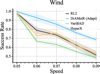
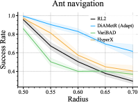
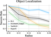
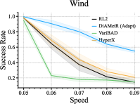
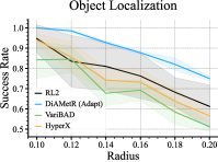
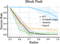
Figure 5: We evaluate DiAMetR and meta RL algorithms ($\text{RL}^{2}$, VariBAD and HyperX) on different in-support (top row) and out-of-support (bottom row) shifted test task distributions. DiAMetR either matches or outperforms $\text{RL}^{2}$, VariBAD and HyperX on these task distributions. The first point $p_{1}$ on the horizontal axis indicates the task parameter ($\Delta$) distribution $\mathcal{U}(0,p_{1})$ and the subsequent points $p_{i}$ indicate task parameter ($\Delta$) distribution $\mathcal{U}(p_{i-1},p_{i})$. While task parameter for wind navigation is wind velocity $w_{\mathcal{T}}$, it is target location $s_{\mathcal{T}}$ for other environments. Table 2 details the task distributions used in this evaluation.

6.2 Analysis of Tasks Proposed by Latent Conditional Uncertainty Sets

We visualize the imagined test reward distribution through their heatmaps for various distribution shifts. To generate an imagined reward function, we sample $z\sim q_{\phi}(z)$ and pass the $z$ into $r_{\omega}(s,a,z)=r_{\omega}(s,z)$ (given the learned reward is only dependent on state as mentioned in Appendix A.1). We then take the agent (for instance the ant) and reset its $(x,y)$ location to different points in the (discretized) grid $[-1,1]^{2}$ and calculate $r_{\omega}(s,z)$ at all those points. This gives us a reward map for a single imagined reward function. We sample $10000$ of these reward functions and plot them together. Figure 6 visualizes the imagined test reward distribution in Ant-navigation environment in increasing order of distribution shifts with respect to train reward distribution (with distribution shift parameter $\epsilon$ increasing from left to right). The train distribution of rewards has uniformly distributed target locations within the red circle. As clearly seen in Figure 6, the learned reward distribution model imagines more target locations outside the red circle as we increase the distribution shifts.

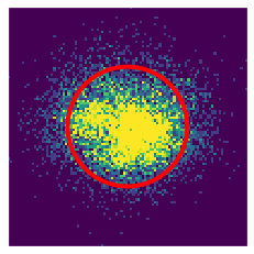
(a) $\epsilon=0.1$

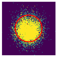
(b) $\epsilon=0.2$

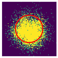
(c) $\epsilon=0.4$

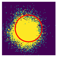
(d) $\epsilon=0.8$

Figure 6: Imagined test reward distributions in Ant-navigation environment in increasing order of distribution shifts. Train reward distribution is uniform within the red circle.

6.3 Analysis of Importance of Multiple Uncertainty Sets

DiAMetR meta-learns a family of adaptation policies, each conditioned on different uncertainty set. As discussed in section 4, selecting a policy conditioned on a large uncertainty set would lead to overly conservative behavior. Furthermore, selecting a policy conditioned on a small uncertainty set would result in failure if the test time distribution shift is high. Therefore, we need to adaptively select an uncertainty set during test time. To validate this phenomenon empirically, we performed an ablation study in Figure 7. As clearly visible, adaptively choosing an uncertainty set during test time allows for better test time distribution adaptation when compared to selecting an uncertainty set beforehand or selecting a large uncertainty set. These results suggest that a combination of training robust meta-learners and constructing various uncertainty sets allows for effective test-time adaptation under distribution shift. DiAMetR  is able to avoid both overly conservative behavior and under-exploration at test-time.

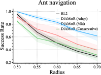
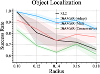
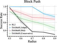
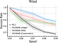
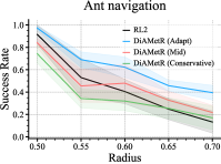
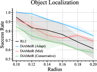
Figure 7: Adaptively choosing an uncertainty set for DiAMetR policy (Adapt) during test time allows it to better adapt to test time distribution shift than choosing an uncertainty set beforehand (Mid). Choosing a large uncertainty set for DiAMetR policy (Conservative) leads to a conservative behavior and hurts its performance when test time distribution shift is low. While top row contains in-support task distribution shifts, the bottom row contains out-of-support task distribution shifts.

7 Discussion

In this work, we discussed the challenge of distribution shift in meta-reinforcement learning and showed how we can build meta-reinforcement learning algorithms that are robust to varying levels of distribution shift. We show how we can build distributionally “adaptive" reinforcement learning algorithms that can adapt to varying levels of distribution shift, retaining a tradeoff between fast learning and maintaining asymptotic performance. We then show we can instantiate this algorithm practically by parameterizing uncertainty sets with a learned generative model. We empirically showed that this allows for learning meta-learners robust to changes in task distribution.

There are several avenues for future work we are keen on exploring, for instance extending adaptive distributional robustness to more complex meta RL tasks, including those with differing transition dynamics. Another interesting direction would be to develop a more formal theory providing adaptive robustness guarantees in meta-RL problems under these inherent distribution shifts.

Author Contributions

Anurag Ajay helped in coming up with the framework of distributionally adaptive meta RL, implemented the DiaMetR algorithm, ran the experiments, helped with writing the paper and led the project.

Abhishek Gupta came up with the framework of distributionally adaptive meta RL, ran initial proof-of-concept experiments, helped with writing the paper and co-led the project.

Dibya Ghosh analyzed the framework of distributionally adaptive meta RL (Section 4.3), wrote all the related proofs, participated in research discussions and helped with writing the paper.

Sergey Levine provided feedback on the work, and participated in research discussions.

Pulkit Agrawal participated in research discussions and advised on the project.

Checklist

1. For all authors…

   1. Do the main claims made in the abstract and introduction accurately reflect the paper’s contributions and scope? [Yes]

   2. Did you describe the limitations of your work? [Yes] See Section 7

   3. Did you discuss any potential negative societal impacts of your work? [N/A] Our work is done in simulation and won’t have any negative societal impact.

   4. Have you read the ethics review guidelines and ensured that your paper conforms to them? [Yes] This work does not actually use human subjects, and is done in simulation. We have reviewed ethics guidelines and ensured that our paper conforms to them.

2. If you are including theoretical results…

   1. Did you state the full set of assumptions of all theoretical results? [N/A] Math is used as a theory/formalism, but we don’t make any provable claims about it.

   2. Did you include complete proofs of all theoretical results? [N/A]

3. If you ran experiments…

   1. Did you include the code, data, and instructions needed to reproduce the main experimental results (either in the supplemental material or as a URL)? [Yes] We have included the code along with a README in the supplemental material

   2. Did you specify all the training details (e.g., data splits, hyperparameters, how they were chosen)? [Yes] See Appendix L

   3. Did you report error bars (e.g., with respect to the random seed after running experiments multiple times)? [Yes] All plots were created with 4 random seeds with std error bars.

   4. Did you include the total amount of compute and the type of resources used (e.g., type of GPUs, internal cluster, or cloud provider)? [Yes] See Appendix L

4. If you are using existing assets (e.g., code, data, models) or curating/releasing new assets…

   1. If your work uses existing assets, did you cite the creators? [Yes] Environments we used are cited in section 6. Codebase used are cited in Appendix L

   2. Did you mention the license of the assets? [N/A]

   3. Did you include any new assets either in the supplemental material or as a URL? [Yes] We published the code and included all environments and assets as a part of this

   4. Did you discuss whether and how consent was obtained from people whose data you’re using/curating? [Yes] Environments and codebases we used are open-source.

   5. Did you discuss whether the data you are using/curating contains personally identifiable information or offensive content? [N/A]

5. If you used crowdsourcing or conducted research with human subjects…

   1. Did you include the full text of instructions given to participants and screenshots, if applicable? [N/A]

   2. Did you describe any potential participant risks, with links to Institutional Review Board (IRB) approvals, if applicable? [N/A]

   3. Did you include the estimated hourly wage paid to participants and the total amount spent on participant compensation? [N/A]

Appendix A DiAMetR for handling out-of-support task distribution shifts

To handle out-of-support task distribution shifts, we parameterized new task distribution as latent space distributions $q_{\phi}(z)$ and measure the divergence between train and test task distribution via KL divergence in latent space $D(p_{\text{train}}(z)||q_{\phi}(z))$ in Section 5. Using this parameterization, equation 3 becomes

$$\max_{\theta} \min_{\phi}\mathbb{E}_{z\sim q_{\phi}(z)}\left[\mathbb{E}_{\pi_{\text{meta},\theta}^{\epsilon},{\mathcal{P}}}\left[\frac{1}{k}\sum_{i=1}^{k}\sum_{t=1}^{T}{\color[rgb]{.75,0,.25}r_{\omega}(s_{t}^{(i)},a_{t}^{(i)},z)}\right]\right]\;\;\;{\color[rgb]{.75,0,.25}\text{when rewards differ}}$$

$$\max_{\theta} \min_{\phi}\mathbb{E}_{z\sim q_{\phi}(z)}\left[\mathbb{E}_{\pi_{\text{meta},\theta}^{\epsilon},{\color[rgb]{.75,.5,.25}p_{\omega}(\cdot,\cdot,z)}}\left[\frac{1}{k}\sum_{i=1}^{k}\sum_{t=1}^{T}r_{t}^{(i)}\right]\right]\;\;\;{\color[rgb]{.75,.5,.25}\text{when dynamics differ}}$$

$$~{}D_{\text{KL}}(p_{\text{train}}(z)||q_{\phi}(z))\leq\epsilon$$ (10)

This objective function is solved in Algorithm 1 for different values of $\epsilon$. To imagine out-of-support distributionally shifted task (i.e. reward or dynamics) distributions, DiAMetR leverages structured VAE which we describe in subsequent subsections.

A.1 Structured VAE for modeling reward distributions

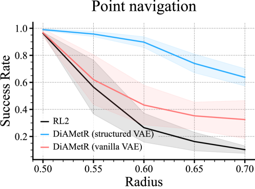
Figure 8: Using a vanilla VAE, in lieu of a structured VAE, to model task distribution hurts DiAMetR’s performance on test-task distributions.

We leverage the sparsity in reward functions (i.e. $0/1$ rewards) in the environments used and describe a structured VAE to model $r_{\omega}(s,a,z)$ with $p(z)={\mathcal{N}}(0,I)$ and KL-divergence for $D(\cdot||\cdot)$. Let $\overline{h}=(\sum_{t=1}^{T}r_{t}s_{t})/(\sum_{t=1}^{T}r_{t})$ be the mean of states achieving a $+1$ reward in trajectory $h$. The encoder $z\sim q_{\psi}(z|\overline{h})$ encodes $\overline{h}$ into a latent vector $z$. The reward model $r_{\omega}(s,a,z)$ consists of 2 components: (i) latent decoder $\hat{\overline{h}}=r^{h}_{\omega}(z)$ which reconstructs $\overline{h}$ and (ii) reward predictor $r^{\text{rew}}_{\omega}(s,\hat{\overline{h}})=\exp(-\|M\odot(s-\hat{\overline{h}})\|_{2}^{2}/\sigma^{2})$ which predicts reward for a state given the decoded latent vector. $M$ is a masking function and $\sigma$ is a learned parameter. The training objective becomes

$$\min_{\omega,\psi}\mathbb{E}_{h\sim{\mathcal{D}}}\left[\mathbb{E}_{z\sim q_{\psi}(z|\overline{h})}\left[\left\|\overline{h}-r^{h}_{\omega}(z)\right\|_{2}^{2}+\sum_{t=1}^{T}\left\|r^{\text{rew}}_{\omega}(s_{t},r^{h}_{\omega}(z))-r_{t}\right\|^{2}\right]+D_{\text{KL}}(q_{\psi}(z|\overline{h})||p(z))\right]$$ (11)

The structure in the VAE helps in extrapolating reward functions when $z\sim q_{\phi}(z)$. This can be further verified by reduction in DiAMetR’s performance on test-task distributions when using vanilla VAE (see Figure 8).

A.2 Structured VAE for modelling dynamics distributions

We describe our structured VAE architecture for modelling dynamics distribution $p_{\omega}(s,a,z)$ with $p(z)={\mathcal{N}}(0,I)$ and KL-divergence for $D(\cdot||\cdot)$. It handles out-of-support shifted test task distributions where only dynamics vary across tasks. We leverage the fact that dynamics differ by an additive term. The encoder $z\sim q_{\phi}(z|(s_{t},a_{t})_{t=1}^{T})$ encodes the state action trajectory to a latent vector $z$. The dynamics model takes the form $p_{\omega}(s,a,z)=W_{\omega}z+p_{\omega}^{\text{dyn}}(s,a)$ where $W_{\omega}$ is a parameter. The training objective becomes:

$$\min_{\omega,\psi}\mathbb{E}_{(s_{t},a_{t})_{t=1}^{T}\sim{\mathcal{D}}}\left[\mathbb{E}_{z\sim q_{\psi}(z|(s_{t},a_{t})_{t=1}^{T})}\left[\sum_{t=1}^{T-1}\left\|p^{\text{dyn}}_{\omega}(s_{t},a_{t})+W_{\omega}z-s_{t+1}\right\|^{2}\right]+D_{\text{KL}}(q_{\psi}(z|(s_{t},a_{t})_{t=1}^{T})||p(z))\right]$$ (12)

The structure in the VAE helps in extrapolating dynamics when $z\sim q_{\phi}(z)$.

Appendix B DiAMetR for handling in-support task distribution shifts

To handle in-support task distribution shifts, we parameterized new task distribution as re-weighted (empirical) training task distribution $q_{\phi}({\mathcal{T}})\propto w_{\mathcal{T}}p_{\text{train}}({\mathcal{T}})$ (where $\phi=\{w_{{\mathcal{T}}_{i}}\}_{i=1}^{n_{\text{tr}}}$) in Section 5. Using this parameterization, equation 3 becomes

$$\max_{\theta} \min_{\phi}\mathbb{E}_{{\mathcal{T}}\sim p_{\text{train}}({\mathcal{T}})}\left[\mathbb{E}_{\pi_{\text{meta},\theta}^{\epsilon},{\mathcal{P}}}\left[\frac{nw_{\mathcal{T}}}{\sum_{i=1}^{n_{\text{tr}}}w_{{\mathcal{T}}_{i}}}\frac{1}{k}\sum_{i=1}^{k}\sum_{t=1}^{T}r_{t}^{(i)}\right]\right]$$

$$~{}D_{\text{KL}}(p_{\text{train}}({\mathcal{T}})||q_{\phi}({\mathcal{T}}))\leq\epsilon$$ (13)

This objective function is solved in Algorithm 1 for different values of $\epsilon$. For in-support task distribution shifts, shifts in dynamics distribution and reward distribution don’t require separate treatment.

Appendix C Test time Meta Policy Selection

Algorithm 3 (Detailed) DiAMetR:Meta-training phase

1:  Given: $p_{\text{train}}({\mathcal{T}})$, Return: $\{\pi_{\text{meta},\theta}^{\epsilon_{i}}\}_{i=1}^{M}$

2:  $\pi_{\text{meta},\theta}^{\epsilon_{1}}$, ${\mathcal{D}}_{\text{Replay-Buffer}}\leftarrow$ Solve equation 1 with off-policy $\text{RL}^{2}$

3:  Reward distribution $r_{\omega}$ / Dynamic distribution $p_{\omega}$, prior $p_{\text{train}}(z)\leftarrow$ Solve eq 8 using ${\mathcal{D}}_{\text{Replay-Buffer}}$

4:  for $\epsilon$ in $\{\epsilon_{2},\ldots,\epsilon_{M}\}$ do

5:    Initialize $q_{\phi}$, $\pi_{\text{meta},\theta}^{\epsilon}$ and $\lambda\geq 0$.

6:    for iteration $n=1,2,...$ do

7:       Meta-policy: Update $\pi_{\text{meta},\theta}^{\epsilon}$ using off-policy $\text{RL}^{2}$ [30]

$$\theta\coloneqq\theta+\alpha\nabla_{\theta}\mathbb{E}_{{\mathcal{T}}\sim p_{\text{train}}({\mathcal{T}})}[\mathbb{E}_{\pi_{\text{meta},\theta}^{\epsilon},{\mathcal{T}}}[\frac{nw_{\mathcal{T}}}{k\sum_{i=1}^{n_{\text{tr}}}w_{{\mathcal{T}}_{i}}}\sum_{i=1}^{k}\sum_{t=1}^{T}r_{t}^{(i)}]]$$

$$\theta\coloneqq\theta+\alpha\nabla_{\theta}\mathbb{E}_{z\sim q_{\phi}(z)}[\mathbb{E}_{\pi_{\text{meta},\theta}^{\epsilon},{\mathcal{P}}}[\frac{1}{k}\sum_{i=1}^{k}\sum_{t=1}^{T}r_{\omega}(s_{t}^{(i)},a_{t}^{(i)},z)]]$$

$$\theta\coloneqq\theta+\alpha\nabla_{\theta}\mathbb{E}_{z\sim q_{\phi}(z)}[\mathbb{E}_{\pi_{\text{meta},\theta}^{\epsilon},p_{\omega}(\cdot,\cdot,z)}[\frac{1}{k}\sum_{i=1}^{k}\sum_{t=1}^{T}r_{t}^{(i)}]]$$

8:       Adversarial task distribution: Update $q_{\phi}$ using Reinforce [38]

$$\phi\coloneqq\phi-\alpha\nabla_{\phi}(\mathbb{E}_{{\mathcal{T}}\sim p_{\text{train}}({\mathcal{T}})}[\mathbb{E}_{\pi_{\text{meta},\theta}^{\epsilon},{\mathcal{T}}}[\frac{nw_{\mathcal{T}}}{k\sum_{i=1}^{n_{\text{tr}}}w_{{\mathcal{T}}_{i}}}\sum_{i=1}^{k}\sum_{t=1}^{T}r_{t}^{(i)}]]+\lambda D_{\text{KL}}(p_{\text{train}}({\mathcal{T}})\|q_{\phi}({\mathcal{T}}))$$

$$\phi\coloneqq\phi-\alpha\nabla_{\phi}(\mathbb{E}_{z\sim q_{\phi}(z)}[\mathbb{E}_{\pi_{\text{meta},\theta}^{\epsilon},{\mathcal{P}}}[\frac{1}{k}\sum_{i=1}^{k}\sum_{t=1}^{T}r_{\omega}(s_{t}^{(i)},a_{t}^{(i)},z)]]+\lambda D_{\text{KL}}(p_{\text{train}}(z)\|q_{\phi}(z))$$

$$\phi\coloneqq\phi-\alpha\nabla_{\phi}(\mathbb{E}_{z\sim q_{\phi}(z)}[\mathbb{E}_{\pi_{\text{meta},\theta}^{\epsilon},p_{\omega}(\cdot,\cdot,z)}[\frac{1}{k}\sum_{i=1}^{k}\sum_{t=1}^{T}r_{t}^{(i)}]]+\lambda D_{\text{KL}}(p_{\text{train}}(z)\|q_{\phi}(z))$$

9:       Lagrange constraint multiplier: Update $\lambda$ to enforce $D_{\text{KL}}(p_{\text{train}}\|q_{\phi})<\epsilon$,

$$\lambda\coloneqq_{\lambda\geq 0}\lambda+\alpha(D_{\text{KL}}(p_{\text{train}}({\mathcal{T}})\|q_{\phi}({\mathcal{T}}))-\epsilon)$$

$${\color[rgb]{.75,0,.25}\lambda\coloneqq_{\lambda\geq 0}\lambda+\alpha(D_{\text{KL}}(p_{\text{train}}(z)\|q_{\phi}(z))-\epsilon)}\;\;\;\;{\color[rgb]{.75,.5,.25}\lambda\coloneqq_{\lambda\geq 0}\lambda+\alpha(D_{\text{KL}}(p_{\text{train}}(z)\|q_{\phi}(z))-\epsilon)}$$

10:    end for

11:  end for

As discussed in Section 4, to adapt to test time task distribution shifts, we train a family of meta-policies $\Pi=\{\pi_{\text{meta}}^{\epsilon_{i}}\}$ to be robust to varying degrees of distribution shifts. We then choose the appropriate meta-policy during test-time based on the inferred task distribution shift. In this section, we frame the test-time selection of meta-policy from the family $\Pi$ as a stochastic multi-arm bandit problem. Every iteration involves pulling an arm $i$ which corresponds to executing $\pi_{\text{meta}}^{\epsilon_{i}}$ for $1$ meta-episode ($k$ environment episodes) on a task ${\mathcal{T}}\sim p_{\text{test}}({\mathcal{T}})$. Let $R_{i}$ be the expected return for pulling arm $i$

$$R_{i}=\mathbb{E}_{\pi_{\text{meta}}^{\epsilon_{i}},{\mathcal{T}}\sim p_{\text{test}}({\mathcal{T}})}\left[\frac{1}{k}\sum_{i=1}^{k}\sum_{t=1}^{T}r_{t}^{(i)}\right]$$ (14)

Let $R^{*}=\max_{i\in\{1,\ldots,M\}}R_{i}$ and $\pi_{\text{meta}}^{\epsilon}$ be the corresponding meta-policy. The goal of the stochastic bandit problem is to pull arms $i_{1},\ldots,i_{N}\in\{1,\ldots,M\}$ such that the test-time regret ${\mathcal{R}}_{N}$ is minimized

$${\mathcal{R}}_{N}^{\text{test}}=NR^{*}-\sum_{t=1}^{N}R_{i_{t}}$$ (15)

with constraint that $i_{t}$ can depend only on the information available prior to iteration $t$. We choose Thompson sampling, a zero-regret bandit algorithm, to solve this problem. In principle, Thompson sampling should learn to choose $\pi_{\text{meta}}^{\epsilon}$ after $N$ iterations.

Appendix D Environment Description

We describe the environments used in the paper:

• {Point,Wheeled,Ant}-navigation: The rewards for each task correspond to reaching an unobserved target location $s_{{\mathcal{T}}}$. The agent (i.e. Wheeled, Ant) must explore the environment to find the unobserved target location (Wheeled driving a differential drive robot, Ant controlling a four legged robotic quadruped). It receives a reward of $1$ once it gets within a small $\delta$ distance of the target $s_{t}$, as in  [13].

• Dense Ant-navigation: The rewards for each task correspond to reaching an unobserved target location $s_{{\mathcal{T}}}$. The Ant (a four legged robotic quadruped) must explore the environment to find the unobserved target location. It receives a reward of $-\|\text{agent}_{x,y}-s_{\mathcal{T}}\|$ where $\text{agent}_{x,y}$ is the (x,y) position of the Ant.

• Wind navigation: The rewards for each task correspond to reaching an unobserved target location $s_{t}$. While $s_{{\mathcal{T}}}$ is fixed across tasks (i.e. at $(1/\sqrt{2},1/\sqrt{2})$), the agent (a linear system robot) much navigate in the presence of wind (i.e. a noise vector $w_{{\mathcal{T}}}$) that varies across tasks. It receives a reward of $1$ once it gets within a small $\delta$ distance of the target $s_{{\mathcal{T}}}$.

• Object localization: Each task corresponds to using the gripper to localize an object kept at an unobserved target location $s_{t}$. The Fetch robot must move its gripper around and explore the environment to find the object. Once the gripper touches the object kept at target location $s_{t}$, it receives a reward of $1$.

• Block push: Each task corresponds to moving the block to an unobserved target location $s_{t}$. The robot arm must move the block around and explore the environment to find the unobserved target location. Once the block gets within a small $\delta$ distance of the target $s_{t}$, it receives a reward of $1$, as in  [13].

Furthermore, Table 1 describes the state space ${\mathcal{S}}$, action space ${\mathcal{A}}$, episodic horizon $H$, frameskip for each environment and $k$ (i.e. number of environment episodes in $1$ meta episode). Table 2 provides parameters for train and test task distributions for different meta-RL tasks used in the paper.

Table 1: Environment Description

Name	State space ${\mathcal{S}}$	Action space ${\mathcal{A}}$	Episodic Horizon $H$	Frameskip	$k$
Point-navigation	Box(2,)	Box(2,)	60	1	2
Wind-navigation	Box(2,)	Box(2,)	25	1	1
Wheeled-navigation	Box(12,)	Box(2,)	60	10	2
Ant-navigation	Box(29,)	Box(8,)	200	5	2
Dense Ant-navigation	Box(29,)	Box(8,)	200	5	2
Object localization	Box(17,)	Box(6,)	50	10	2
Block Push	Box(10,)	Box(4,)	60	10	2

Table 2: Parameters for train and test task distribution for {Point,Wheeled, Ant}-navigation, Dense Ant-navigation, Wind-navigation, Object localization and Block-push. While tasks in Wind-navigation vary in dynamics, tasks in other environments vary in reward function. The shifted test task distributions can be either in-support or out-of-support of the training task distribution. All these task distributions are determined by distributions of underlying task parameters (say target location $s_{\mathcal{T}}$ or wind velocity $w_{\mathcal{T}}$), which either determine the reward function or the dynamics function.

Environment	Task type	Task parameter distribution	$p_{\text{train}}({\mathcal{T}})$	$\{p_{\text{test}}^{i}({\mathcal{T}})\}_{i=1}^{K}$
Point, Wheeled, Ant-navigation	reward change, out-of-support shift	$s_{\mathcal{T}}=(\Delta\cos\theta,\Delta\sin\theta)$ $\Delta\sim\mathcal{U}(\Delta_{\min},\Delta_{\max})$ $\theta\sim\mathcal{U}(0,2\pi)$	$\Delta\sim\mathcal{U}(0,0.5)$	$\Delta\sim\mathcal{U}(0,0.5),\mathcal{U}(0.5,0.55)$ $\mathcal{U}(0.55,0.6),\mathcal{U}(0.6,0.65)$ $\mathcal{U}(0.65,0.7)$
Point, Wheeled, Ant-navigation	reward change, in-support shift	$s_{\mathcal{T}}=(\Delta\cos\theta,\Delta\sin\theta)$ $\Delta\sim\mathcal{U}(\Delta_{\min},\Delta_{\max})$ $\theta\sim\mathcal{U}(0,2\pi)$	$\Delta\sim\text{Exp}(\lambda=5)$	$\Delta\sim\mathcal{U}(0,0.5),\mathcal{U}(0.5,0.55)$ $\mathcal{U}(0.55,0.6),\mathcal{U}(0.6,0.65)$ $\mathcal{U}(0.65,0.7)$
Dense Ant-navigation	reward change, in-support shift	$s_{\mathcal{T}}=(\Delta\cos\theta,\Delta\sin\theta)$ $\Delta\sim\mathcal{U}(\Delta_{\min},\Delta_{\max})$ $\theta\sim\mathcal{U}(0,2\pi)$	$\Delta\sim\text{Exp}(\lambda=5)$	$\Delta\sim\mathcal{U}(0,0.5),\mathcal{U}(0.5,0.55)$ $\mathcal{U}(0.55,0.6),\mathcal{U}(0.6,0.65)$ $\mathcal{U}(0.65,0.7)$
Wind -navigation	dynamics change, out-of-support shift	$w_{\mathcal{T}}=(\Delta\cos\theta,\Delta\sin\theta)$ $\Delta\sim\mathcal{U}(\Delta_{\min},\Delta_{\max})$ $\theta\sim\mathcal{U}(0,2\pi)$	$\Delta\sim\mathcal{U}(0,0.05)$	$\Delta\sim\mathcal{U}(0,0.05),\mathcal{U}(0.05,0.06)$ $\mathcal{U}(0.06,0.07),\mathcal{U}(0.07,0.08)$ $\mathcal{U}(0.08,0.09)$
Wind -navigation	dynamics change, in-support shift	$w_{\mathcal{T}}=(\Delta\cos\theta,\Delta\sin\theta)$ $\Delta\sim\mathcal{U}(\Delta_{\min},\Delta_{\max})$ $\theta\sim\mathcal{U}(0,2\pi)$	$\Delta\sim\text{Exp}(\lambda=40)$	$\Delta\sim\mathcal{U}(0,0.05),\mathcal{U}(0.05,0.06)$ $\mathcal{U}(0.06,0.07),\mathcal{U}(0.07,0.08)$ $\mathcal{U}(0.08,0.09)$
Object localization	reward change, out-of-support shift	$s_{\mathcal{T}}=(\Delta\cos\theta,\Delta\sin\theta)$ $\Delta\sim\mathcal{U}(\Delta_{\min},\Delta_{\max})$ $\theta\sim\mathcal{U}(0,2\pi)$	$\Delta\sim\mathcal{U}(0,0.1)$	$\Delta\sim\mathcal{U}(0,0.1),\mathcal{U}(0.1,0.12)$ $\mathcal{U}(0.12,0.14),\mathcal{U}(0.14,0.16)$ $\mathcal{U}(0.16,0.18),\mathcal{U}(0.18,0.2)$
Object localization	reward change, in-support shift	$s_{\mathcal{T}}=(\Delta\cos\theta,\Delta\sin\theta)$ $\Delta\sim\mathcal{U}(\Delta_{\min},\Delta_{\max})$ $\theta\sim\mathcal{U}(0,2\pi)$	$\Delta\sim\text{Exp}(\lambda=20)$	$\Delta\sim\mathcal{U}(0,0.1),\mathcal{U}(0.1,0.12)$ $\mathcal{U}(0.12,0.14),\mathcal{U}(0.14,0.16)$ $\mathcal{U}(0.16,0.18)$
Block-push	reward change, out-of-support shift	$s_{\mathcal{T}}=(\Delta\cos\theta,\Delta\sin\theta)$ $\Delta\sim\mathcal{U}(\Delta_{\min},\Delta_{\max})$ $\theta\sim\mathcal{U}(0,\pi/2)$	$\Delta\sim\mathcal{U}(0,0.5)$	$\Delta\sim\mathcal{U}(0,0.5),\mathcal{U}(0.5,0.6)$ $\mathcal{U}(0.6,0.7),\mathcal{U}(0.7,0.8)$ $\mathcal{U}(0.8,0.9),\mathcal{U}(0.9,1.0)$
Block-push	reward change, in-support shift	$s_{\mathcal{T}}=(\Delta\cos\theta,\Delta\sin\theta)$ $\Delta\sim\mathcal{U}(\Delta_{\min},\Delta_{\max})$ $\theta\sim\mathcal{U}(0,\pi/2)$	$\Delta\sim\text{Exp}(\lambda=4)$	$\Delta\sim\mathcal{U}(0,0.5),\mathcal{U}(0.5,0.6)$ $\mathcal{U}(0.6,0.7),\mathcal{U}(0.7,0.8)$ $\mathcal{U}(0.8,0.9),\mathcal{U}(0.9,1.0)$

Appendix E Experimental Evaluation on Wheeled and Point Robot Navigation

In Section 6, we evaluated DiAMetR on Wind-navigation, Ant-navigation, Fetch-reach and Block-push. We continue the experimental evaluation of DiAMetR in this section and compare it to $\text{RL}^{2}$, VariBAD, and HyperX on train task distribution and different test task distributions of Point navigation and Wheeled navigation [13]. We see that DiAMetR either matches or outperforms the baselines on train task distribution and outperforms the baselines on test task distributions. Furthermore, adaptively selecting an uncertainty set during test time allows for better test time distribution adaptation when compared to selecting an uncertainty set beforehand or selecting a large uncertainty set.

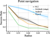
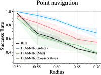
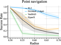
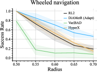
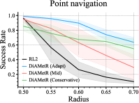
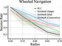
Figure 9: We evaluate DiAMetR and meta RL algorithms ($\text{RL}^{2}$, VariBAD and HyperX) on different in-support and out-of-support shifted test task distribution of Point navigation and Wheeled navigation. DiAMetR either matches or outperforms $\text{RL}^{2}$, VariBAD and HyperX on these task distributions. Furthermore, adaptively selecting an uncertainty set of DiAMetR policy (Adapt) during test time allows it to better adapt to test time distribution shift than choosing an uncertainty set beforehand (Mid). Choosing a large uncertainty set of DiAMetR policy (Conservative) leads to a conservative behavior and hurts its performance when test time distribution shift is low. The first point $p_{1}$ on the horizontal axis indicates the task parameter ($\Delta$) distribution $\mathcal{U}(0,p_{1})$ and the subsequent points $p_{i}$ indicate task parameter ($\Delta$) distribution $\mathcal{U}(p_{i-1},p_{i})$. Here, task parameter is target location $s_{\mathcal{T}}$. Table 2 details the task distributions used in this evaluation.

Appendix F Evaluations on dense reward environments with in-support distribution shifts

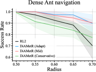
Figure 10: We evaluate DiAMetR and meta RL algorithms ($\text{RL}^{2}$, VariBAD and HyperX) on different in-support shifted test task distributions of Dense Ant-navigation. DiAMetR either matches or outperforms $\text{RL}^{2}$, VariBAD and HyperX on these test task distributions. Furthermore, selecting a single uncertainty set (that is neither too small nor too large) is sufficient in Dense Ant-navigation as DiAMetR(Adapt) and DiAMetR(Mid) have similar performances (within standard error). The first point $p_{1}$ on the horizontal axis indicates the task target distance ($\Delta$) distribution $\mathcal{U}(0,p_{1})$ and the subsequent points $p_{i}$ indicate task target distance ($\Delta$) distribution $\mathcal{U}(p_{i-1},p_{i})$.

We test the applicability of DiAMetR on an environment with dense rewards. We use a variant of Ant navigation, namely Dense Ant-navigation for this evaluation. Furthermore, the shifted test task distributions are in-support of the training task distribution (see Table 2 for a detailed description of these task distributions). Figure 10 shows that DiAMetR still outperforms existing meta RL algorithms ($\text{RL}^{2}$, VariBAD, HyperX) on shifted test task distributions. However, the gap between DiAMetR and other meta RL algorithms is less than in sparse reward environments. Furthermore, Figure 10 shows that selecting a single uncertainty set (that is neither too small nor too large) is sufficient in Dense Ant-navigation as DiAMetR(Adapt) and DiAMetR(Mid) have similar performances (within standard error).

Appendix G Meta-policy Selection and Adaptation during Meta-test

In this section, we show that DiAMetR is able adapt to various test task distributions across different environments by selecting an appropriate meta-policy based on the inferred test-time distribution shift and then quickly adapting the meta-policy to new tasks drawn from the same test-distribution. The performance of meta-RL baselines ($\text{RL}^{2}$, variBAD, HyperX) remains more or less the same after test-time finetuning showing that $10$ iteration (with $25$ rollouts per iteration) isn’t enough for the meta-RL baselines to adapt to a new task distribution. For comparison, these meta-RL baselines take 1500 iterations (with 25 meta-episodes per iteration) during training to learn a meta-policy for train task distribution.

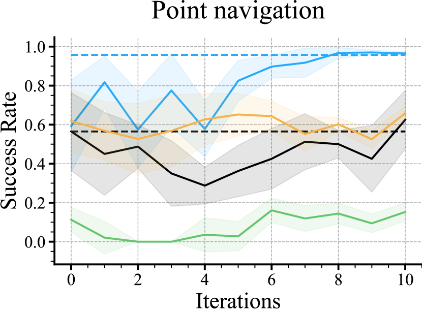
(a) $\Delta\sim\mathcal{U}(0.5,0.55)$

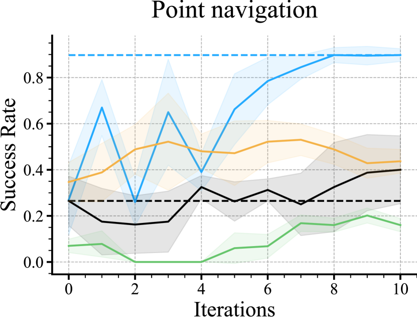
(b) $\Delta\sim\mathcal{U}(0.55,0.6)$

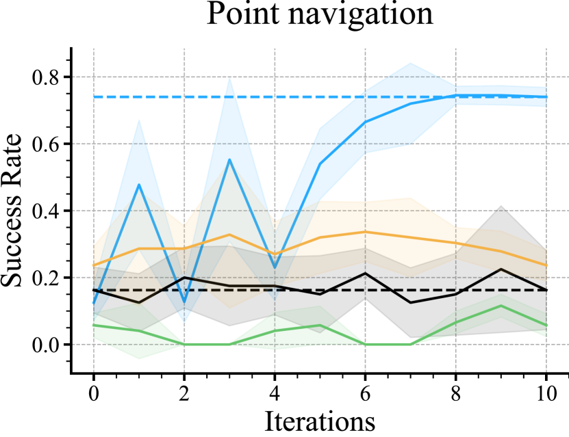
(c) $\Delta\sim\mathcal{U}(0.6,0.65)$

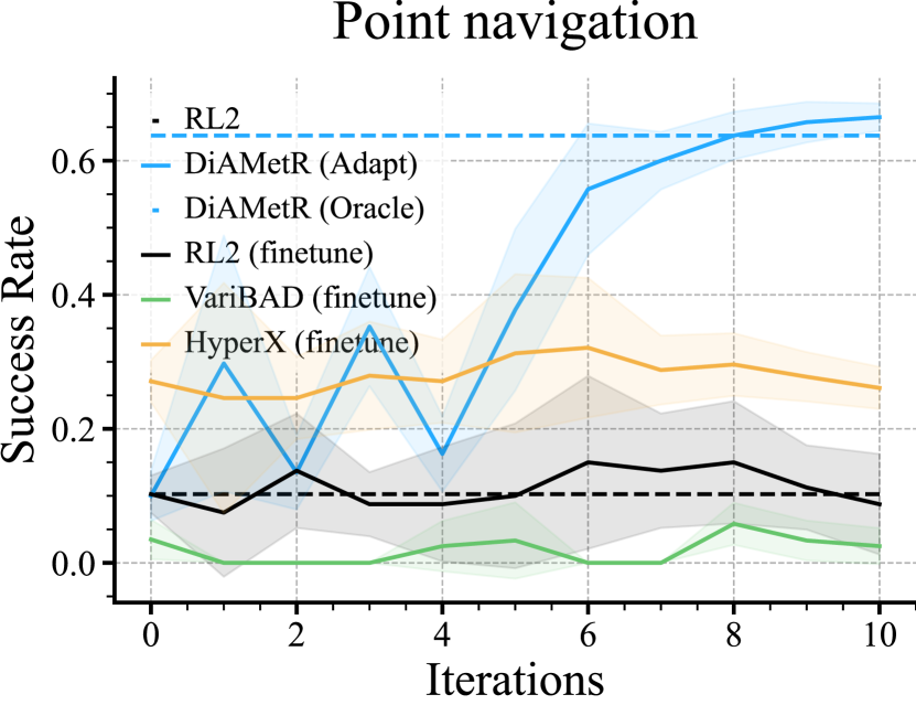
(d) $\Delta\sim\mathcal{U}(0.65,0.7)$

Figure 11: We compare test time adaptation of DiAMetR with test time finetuning of $\text{RL}^{2}$ on point robot navigation for various test task distributions. We run the adaptation procedure for $10$ iterations collecting $25$ rollouts per iteration.

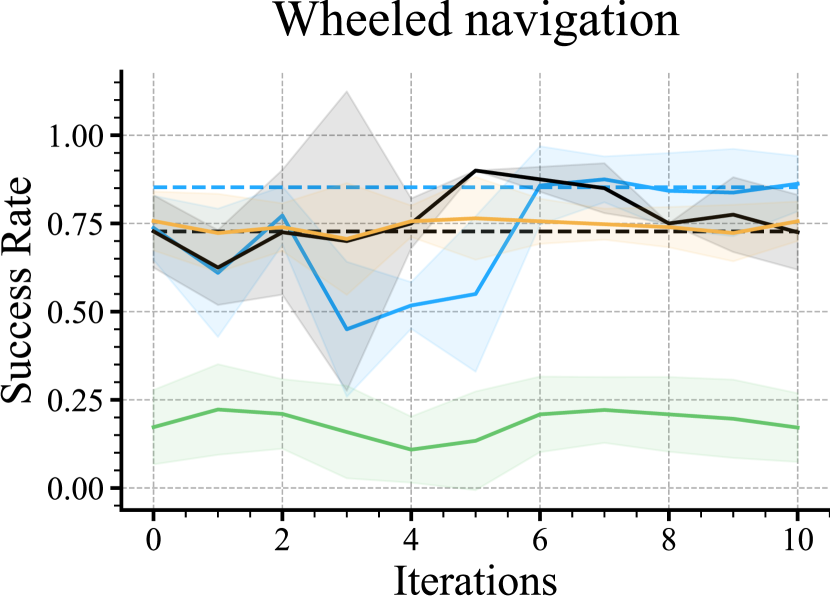
(a) $\Delta\sim\mathcal{U}(0.5,0.55)$

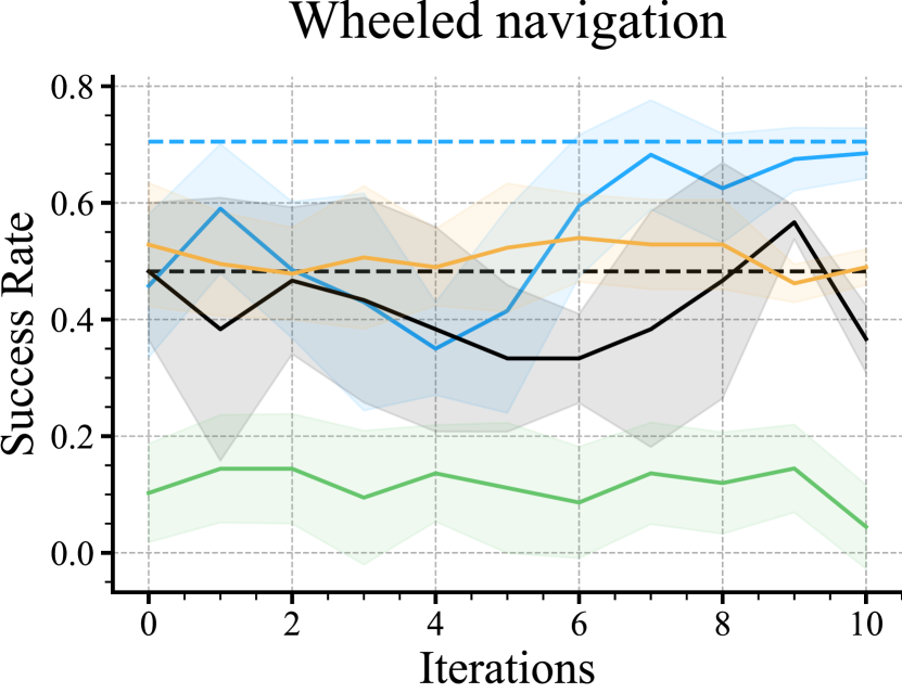
(b) $\Delta\sim\mathcal{U}(0.55,0.6)$

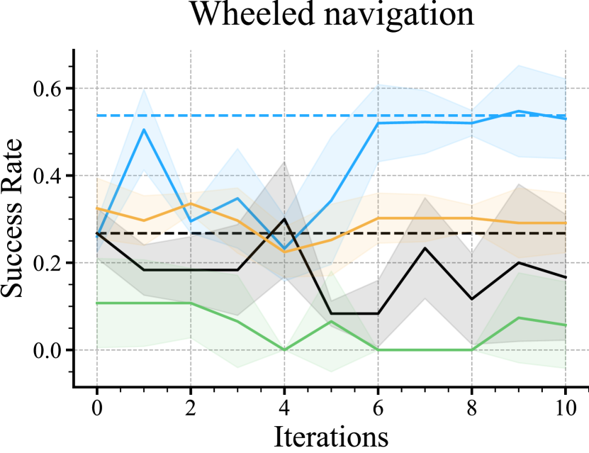
(c) $\Delta\sim\mathcal{U}(0.6,0.65)$

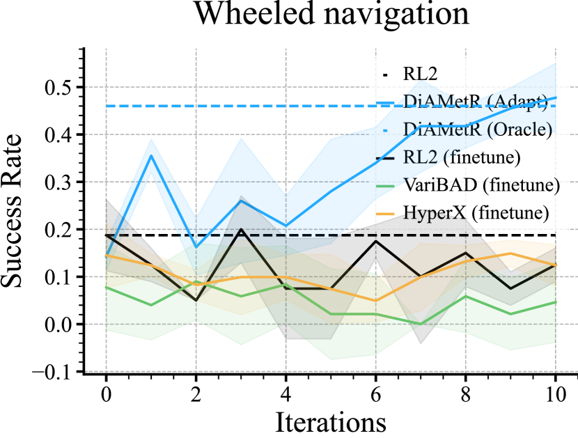
(d) $\Delta\sim\mathcal{U}(0.65,0.7)$

Figure 12: We compare test time adaptation of DiAMetR with test time finetuning of $\text{RL}^{2}$ on wheeled navigation for various test task distributions. We run the adaptation procedure for $10$ iterations collecting $25$ rollouts per iteration.

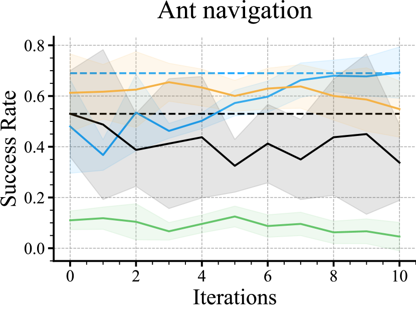
(a) $\Delta\sim\mathcal{U}(0.5,0.55)$

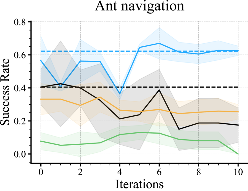
(b) $\Delta\sim\mathcal{U}(0.55,0.6)$

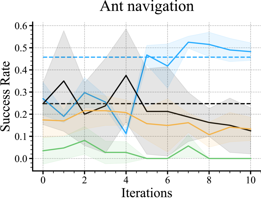
(c) $\Delta\sim\mathcal{U}(0.6,0.65)$

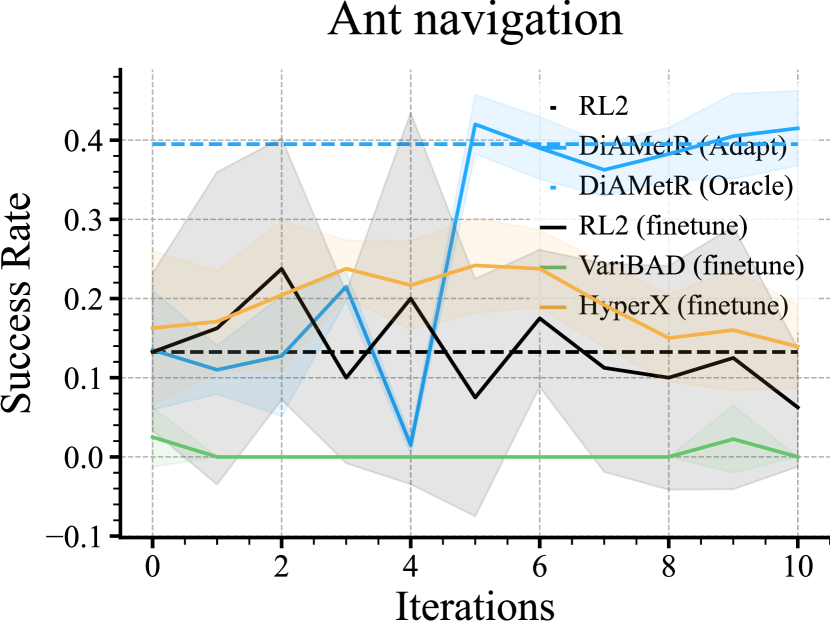
(d) $\Delta\sim\mathcal{U}(0.65,0.7)$

Figure 13: We compare test time adaptation of DiAMetR with test time finetuning of $\text{RL}^{2}$ on ant navigation for various test task distributions. We run the adaptation procedure for $10$ iterations collecting $25$ rollouts per iteration.

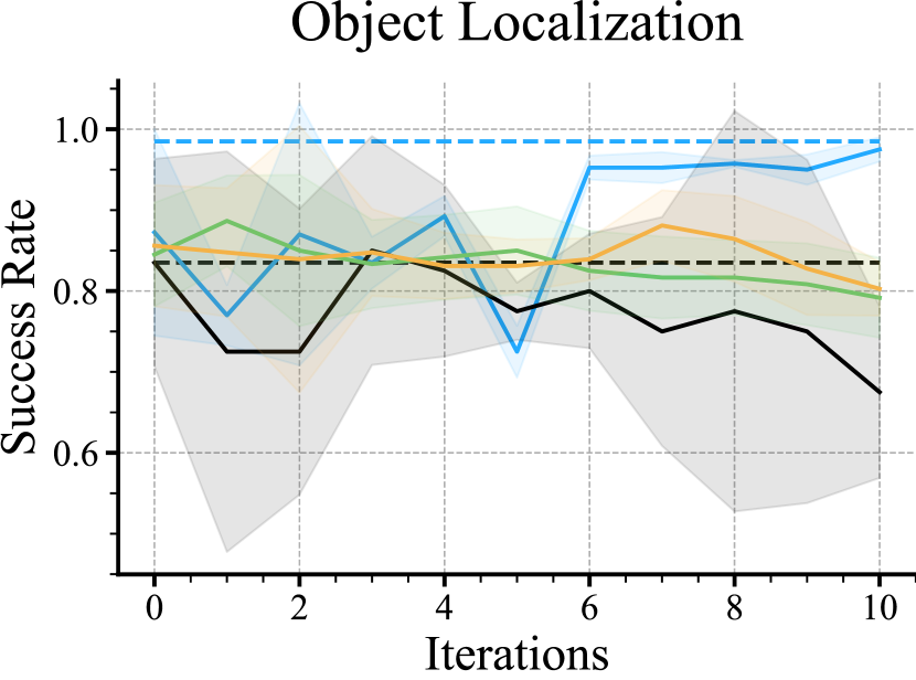
(a) $\Delta\sim\mathcal{U}(0.1,0.12)$

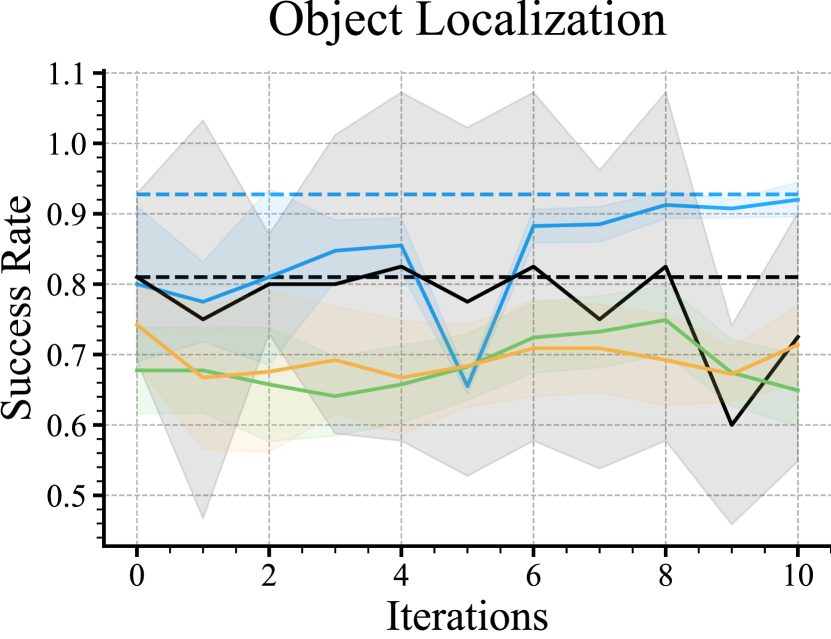
(b) $\Delta\sim\mathcal{U}(0.12,0.14)$

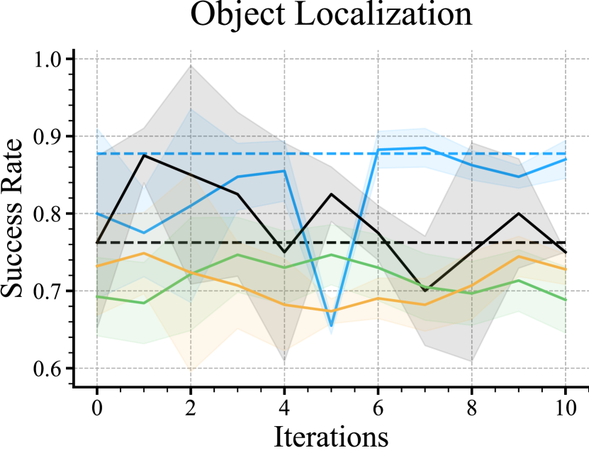
(c) $\Delta\sim\mathcal{U}(0.14,0.16)$

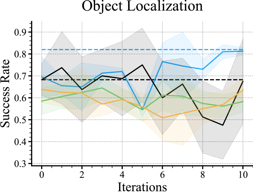
(d) $\Delta\sim\mathcal{U}(0.16,0.18)$

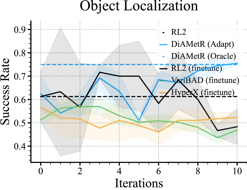
(e) $\Delta\sim\mathcal{U}(0.18,0.20)$

Figure 14: We compare test time adaptation of DiAMetR with test time finetuning of $\text{RL}^{2}$ on object localization for various test task distributions. We run the adaptation procedure for $10$ iterations collecting $25$ rollouts per iteration.

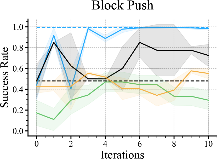
(a) $\Delta\sim\mathcal{U}(0.5,0.6)$

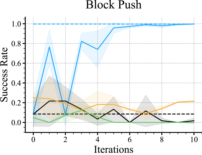
(b) $\Delta\sim\mathcal{U}(0.6,0.7)$

(c) $\Delta\sim\mathcal{U}(0.7,0.8)$

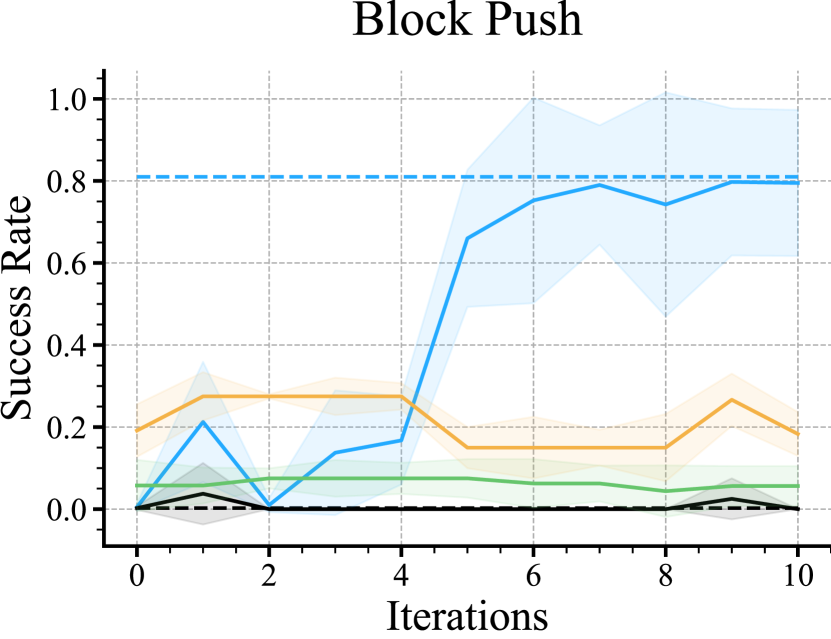
(d) $\Delta\sim\mathcal{U}(0.8,0.9)$

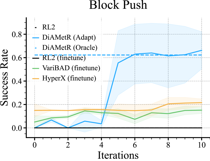
(e) $\Delta\sim\mathcal{U}(0.9,1.0)$

Figure 15: We compare test time adaptation of DiAMetR with test time finetuning of $\text{RL}^{2}$ on block push for various test task distributions. We run the adaptation procedure for $10$ iterations collecting $25$ rollouts per iteration.

Appendix H Ablation studies

Can meta RL achieve robustness to task distribution shifts with improved meta-exploration?

To test if improved meta-exploration can help meta-RL algorithm achieve robustness to test-time task distribution shifts, we test HyperX [49] on test-task distributions in different environments. HyperX leverages curiosity-driven exploration to visit novel states for improved meta-exploration during meta-training. Despite improved meta-exploration, HyperX fails to adapt to test-time task distribution shifts (see Figure 5 and Figure 9 for results on results on different environments). This is because HyperX aims to minimize regret on train-task distribution and doesn’t leverage the visited novel states to learn new behaviors helpful in adapting to test-time task distribution shifts. Furthermore, we note that the contributions of HyperX is complementary to our contributions as improved meta-exploration would help us better learn robust meta-policies.

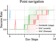
Figure 16: Both SAC trained from scratch (SAC scratch) and SAC pre-trained on training task distribution (SAC finetune) take more than a million timesteps to solve test tasks. In comparison, DiAMetR takes $30k$ timesteps to select the right meta-policy which then solves new tasks from test distribution in $k-1$ environment episodes (i.e. $60$ timesteps given $k=2$ and horizon $H=60$).

Can RL quickly solve test time tasks?

To test if RL can quickly solve test-time tasks, we train Soft Actor Critic (SAC) [14] on $5$ tasks sampled from a particular test task distribution. To make the comparison fair, we include a baseline that pre-trains SAC on train-task distribution. Figure 16 shows results on Point-navigation. We see that both SAC trained from scratch and SAC pre-trained on training task distribution take more than a million timesteps to solve test tasks. In comparison, DiAMetR takes $30k$ timesteps to select the right meta-policy which then solves new tasks from test distribution in $k-1$ environment episodes (i.e. $60$ timesteps given $k=2$ and horizon $H=60$). This shows that meta-RL formulation is required for quick-adaptation to test tasks.

Appendix I Learning meta-policies with different support

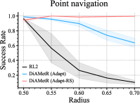
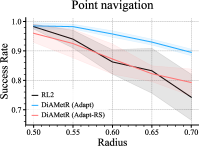
Figure 17: We investigate if learning meta-policies with different support (DiAMetR(Adapt-RS)) is better than learning meta-policies with overlapping support (DiAMetR(Adapt)). We evaluate it on two different families of shifted task distributions. While the left figure shows evaluations on shifted task distributions with different support (i.e. $\mathcal{U}(0,0.5)$, $\mathcal{U}(0.5,0.55)$, $\mathcal{U}(0.55,0.6)$, $\mathcal{U}(0.6,0.65)$, $\mathcal{U}(0.65,0.7)$), the right figure shows evaluations on shifted task distributions with overlapping support (i.e. $\mathcal{U}(0,0.55)$, $\mathcal{U}(0.0,0.6)$, $\mathcal{U}(0.0,0.65)$, $\mathcal{U}(0.0,0.7)$). While DiAMetR(Adapt-RS) performs the best on shifted task distributions with different support, DiAMetR(Adapt) performs the best on shifted task distributions with overlapping support. Hence, whether meta-policies should have overlapping support depends on the nature of shifted test task distributions.

We can alternatively try to learn multiple meta-policies, each with small and different (but slightly overlapping) support. In this way, there won’t be any conservativeness tradeoff. To analyze this further, we focus on point navigation domain (with train target distance distribution as $\Delta\sim{\mathcal{U}}(0,0.5)$) and experiment with out-of-support test task distribution.

Let’s say we are learning the $i^{\text{th}}$ meta-policy (corresponding to $\epsilon_{i}$). Let $q_{\phi}^{i-1}(z)=\mathcal{N}(\mu^{i-1},\sigma^{i-1})$ be the learned adversarial task distribution for $(i-1)^{\text{th}}$ meta-policy (corresponding to $\epsilon_{i-1}$). To learn meta-policies with small and different support, we make 2 changes to Algorithm 1:

1. In step $7$, we do a rejection sampling $z\sim q_{\phi}(z)$ with the condition that $\log q_{\phi}^{i-1}(z)\leq\beta$ (where $\beta$ is a hyperparameter. We found $\beta=-45$ to work well).

2. In step $8$ and $9$, we add another constraint that $D_{\text{KL}}(p_{\text{train}}(z)||q_{\phi}(z))\geq\epsilon_{i-1}$ (in addition to $D_{\text{KL}}(p_{\text{train}}(z)||q_{\phi}(z))\leq\epsilon_{i}$). This leads to learning of two weighting factors $\lambda_{1}$ and $\lambda_{2}$ (instead of just $\lambda$) that tries to ensure $D_{\text{KL}}(p_{\text{train}}(z)||q_{\phi}(z))\in(\epsilon_{i-1},\epsilon_{i})$. We call this modified algorithm as DiAMetR (Adapt-RS) (where RS comes from rejection sampling).

The performance of this variant depends heavily on the form of the test task distribution. We first test it on task target distance distributions $\mathcal{U}(0,0.5),\mathcal{U}(0.5,0.55),\mathcal{U}(0.55,0.6),\mathcal{U}(0.6,0.65),\mathcal{U}(0.65,0.7)$ (essentially testing on rings of disjoint support around the training distribution). We see that DiAMetR(Adapt-RS) maintains a consistent success rate of $\sim 1$ across various target task distributions and outperforms DiAMetR(Adapt) and $\text{RL}^{2}$. This is because each meta-policy has overall smaller (hence are less conservative) and mostly different support and for this type of test distribution, this scheme can be very effective.

However, when we test it on task target distance distributions $\mathcal{U}(0,0.5),\mathcal{U}(0,0.55),\mathcal{U}(0.0,0.6),\mathcal{U}(0.0,0.65),\mathcal{U}(0.0,0.7)$ (essentially testing on discs which mostly include the training distribution), we see that DiAMetR(Adapt-RS) performs same as $\text{RL}^{2}$ and mostly relies on the base $\text{RL}^{2}$ (i.e. $\epsilon=0$) for its performance.

Whether meta-policies should have overlapping support will depend on the nature of shifted test task distributions. If supports of test task distributions overlap, then it’s better to have meta-policies with overlapping support. Otherwise, it’s more efficient to have meta-policies with different support.

Appendix J Meta-policy Selection with CEM during Meta-test

We explore using Cross-entropy method (CEM) [4] for meta-policy selection during meta-test phase, as an alternative to Thompson’s sampling. Algorithm 4 details the use of the CEM algorithm for meta-policy selection. For this evaluation, we use point navigation environment where tasks vary in reward functions and test task distribution is out-of-support of training task distribution. Table 2 provides detailed information about these train and test task distributions. Figure 18 shows that CEM has similar performance as Thompson’s sampling.

Algorithm 4 DiAMetR: Meta-test phase with CEM

1:  Given: $p_{\text{test}}({\mathcal{T}})$, $\Pi=\{\pi_{\text{meta},\theta}^{\epsilon_{i}}\}_{i=1}^{M}$

2:  Sample $\pi\sim\Pi$ (with uniform probability) to collect $25$ meta-episodes

3:  Calculate $(\mu_{\epsilon},\sigma_{\epsilon})$ using $10$ (of $25$) (i.e. top $40$%) meta-episodes with highest returns

4:  for iter $t=2,3,...,10$ do

5:    for meta-episode $n=1,2,..,25$ do

6:       Sample $\epsilon\sim{\mathcal{N}}(\mu_{\epsilon},\sigma_{\epsilon})$

7:       Choose $\epsilon_{i}$ closest to $\epsilon$

8:       Run $\pi_{\text{meta},\theta}^{\epsilon_{i}}$ for meta-episode

9:    end for

10:    Calculate $(\mu_{\epsilon},\sigma_{\epsilon})$ using $10$ (of $25$) (i.e. top $40$%) meta-episodes with highest returns

11:  end for

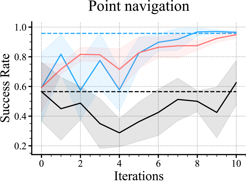
(a) $\Delta\sim\mathcal{U}(0.5,0.55)$

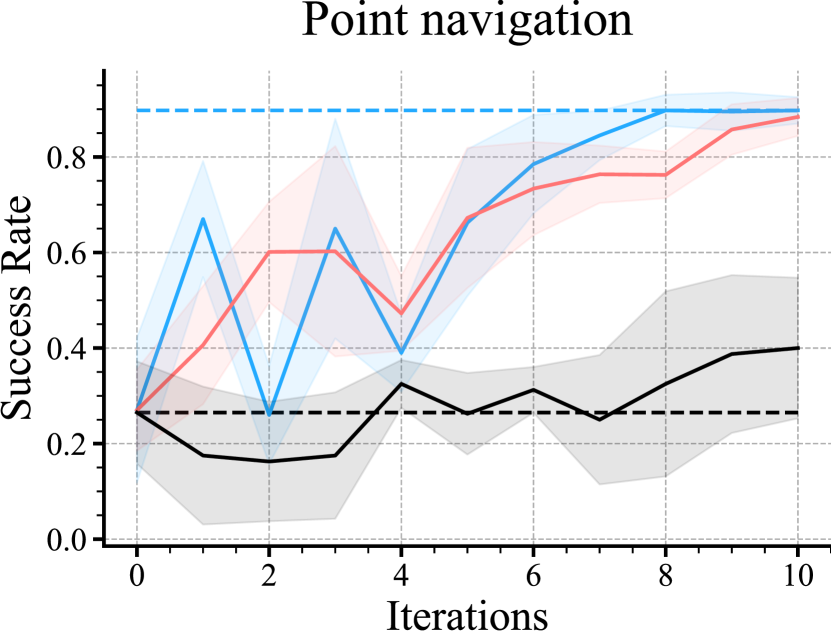
(b) $\Delta\sim\mathcal{U}(0.55,0.6)$

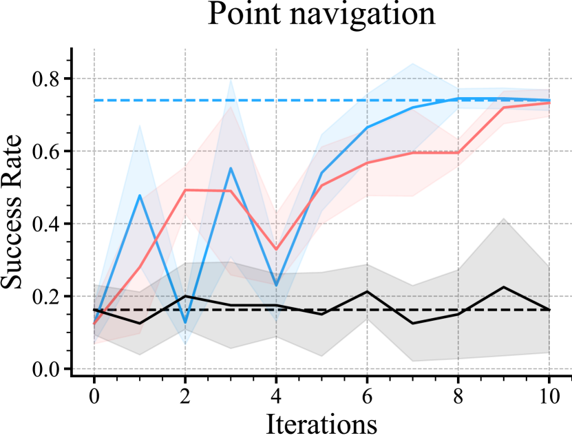
(c) $\Delta\sim\mathcal{U}(0.6,0.65)$

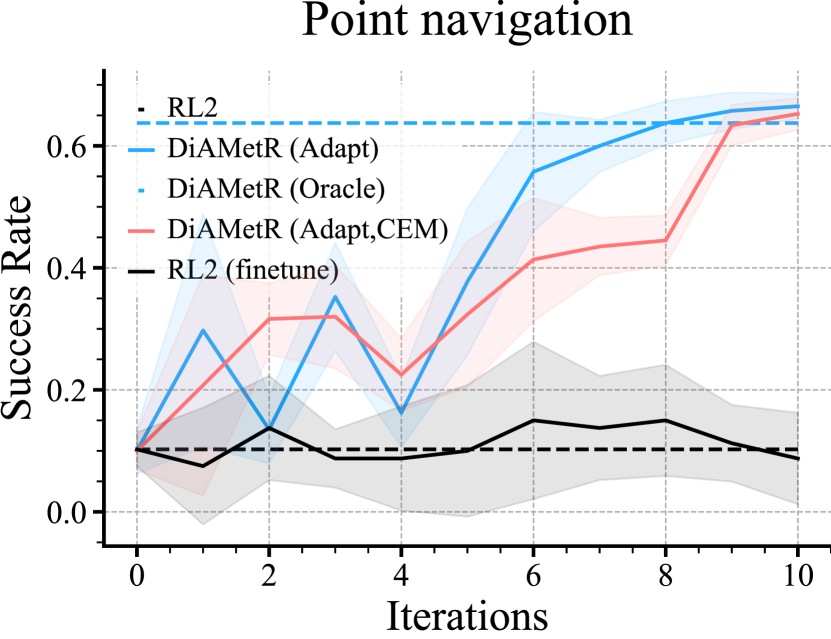
(d) $\Delta\sim\mathcal{U}(0.65,0.7)$

Figure 18: We compare use of Thompson’s sampling (DiAMetR(Adapt)) and Cross-entropy method (DiAMetR(Adapt, CEM)) for test time adaptation of DiAMetR on point robot navigation for various test task distributions. While they have similar performance, they are both better than test-time finetuning of $\text{RL}^{2}$. We run the adaptation procedure for $10$ iterations collecting $25$ rollouts per iteration.

Appendix K Proof of Proposition 4.1

In this section, we prove the proposition in the main text about the excess regret of an $\epsilon_{2}$-robust policy under and $\epsilon_{1}$-perturbation (restated below).

See 4.1

Summary of proof: The proof proceeds in three stages: 1) deriving a form for the optimal meta-policy for a fixed task distribution 2) proving that the optimal $\epsilon$-robust meta-policy takes form:

$$\pi_{\text{meta}}^{\epsilon}(s)\propto\begin{cases}\sqrt{\frac{1-\overline{\epsilon}}{|{\mathcal{S}}_{0}|}}&s\in{\mathcal{S}}_{0}\\ \sqrt{\frac{\overline{\epsilon}}{|{\mathcal{S}}|-|{\mathcal{S}}_{0}|}}&s\notin{\mathcal{S}}_{0}\end{cases}$$

and finally 3) showing that under the task distribution $p({\mathcal{T}}_{g})=(1-\overline{\epsilon_{1}})\text{Uniform}({\mathcal{S}}_{0})+\overline{\epsilon_{1}}\text{Uniform}({\mathcal{S}}\backslash{\mathcal{S}}_{0})$, the gap in regret takes the form in the proposition.

Proof.

For convenience, denote ${\mathcal{S}}_{1}={\mathcal{S}}\backslash{\mathcal{S}}_{0}$ and $\operatorname{Regret}(\pi_{\text{meta}},q({\mathcal{T}}))=\mathbb{E}_{q}[\operatorname{Regret}(\pi,{\mathcal{T}})]$. Furthermore, since the performance of a meta-policy depends only on its final-timestep visitation distribution (and any such distribution is attainable), we directly refer to $\pi(g)$ as the visited goal distribution of the meta-policy $\pi_{\text{meta}}$. Recall that the regret of $\pi_{\text{meta}}$ on task ${\mathcal{T}}_{g}$ is given by $\frac{1}{\pi(g)}$.

We begin with the following lemma that demonstrates the optimal policy for a fixed task distribution.

Lemma K.1.

The optimal meta-policy $\pi_{q}^{*}=\operatorname*{arg\,min}_{\pi}\operatorname{Regret}(\pi,q({\mathcal{T}}_{g}))$ for a given task distribution $q({\mathcal{T}}_{g})$ is given by

$$\pi_{q}^{*}(g)=\frac{1}{\int\sqrt{q(g^{\prime})}\,dg^{\prime}}\sqrt{q(g)}$$ (16)

The proof of the lemma is similar to the argument in Gupta et al. [12], Lee et al. [19]:

$$\pi_{q}^{*} =\operatorname*{arg\,min}_{\pi(g)}\operatorname{Regret}(\pi,q({\mathcal{T}}_{g}))=\operatorname*{arg\,min}_{\pi(g)}\mathbb{E}_{{\mathcal{T}}_{g}\sim q}[\frac{1}{\pi(g)}]$$ (17)

Letting $$Z=\int_{g}\sqrt{q(g)} f f(x)=\frac{1}{x}$$, we can rewrite the optimization problem as minimizing an -divergence (with )

$$=\int\frac{1}{\pi(g)}q(g)\,dg$$ (18)

$$=Z^{2}\int\frac{\sqrt{q(g)}/Z}{\pi(g)}\sqrt{q(g)}/Z\,dg$$ (19)

$$=Z^{2}D_{f}(\pi\|\sqrt{q}(g)/Z)$$ (20)

This is minimized when both are equal, i.e. when $\pi_{q}^{*}(g)=\sqrt{q}/Z$, concluding the proof.

Lemma K.2.

The optimal $\epsilon$-robust meta-policy $\pi^{*\epsilon}=\operatorname*{arg\,min}{\mathcal{R}}(\pi,p_{\text{train}},\epsilon)$ takes form

$$\pi^{\epsilon}(g)\propto\begin{cases}\sqrt{\frac{1-\overline{\epsilon}}{|{\mathcal{S}}_{0}|}}&g\in{\mathcal{S}}_{0}\\ \sqrt{\frac{\overline{\epsilon}}{|{\mathcal{S}}|-|{\mathcal{S}}_{0}|}}&g\notin{\mathcal{S}}_{0}\end{cases}$$

Define the distribution $q^{\epsilon}({\mathcal{T}}_{g})=(1-\overline{\epsilon})\text{Uniform}({\mathcal{S}}_{0})+\overline{\epsilon}\text{Uniform}({\mathcal{S}}\backslash{\mathcal{S}}_{0})$ , which is an $\epsilon$-perturbation of $p_{\text{train}}$ under the TV metric. We note that there are two main cases: 1) if $\overline{\epsilon}=1-\frac{|{\mathcal{S}}_{0}|}{|{\mathcal{S}}|}$, then $q^{\epsilon}$ is uniform over the entire state space, and otherwise 2) it corresponds to uniformly taking $\epsilon$-mass from ${\mathcal{S}}_{0}$ and uniformly distributing it across ${\mathcal{S}}_{1}$. Using the lemma, we can derive the optimal policy for $q^{\epsilon}$, which we denote $\pi^{\epsilon}$:

$$\pi^{\epsilon} =\operatorname*{arg\,min}_{\pi(g)}\operatorname{Regret}(\pi,q^{\epsilon}({\mathcal{T}}))=\frac{1}{\int\sqrt{q^{\epsilon}(g^{\prime})}\,dg^{\prime}}\sqrt{q(g)},$$ (21)

Writing $$Z_{\epsilon}=\int\sqrt{q(g^{\prime})}\,dg^{\prime}$$, we can write this explicitly as

$$=\frac{1}{Z_{\epsilon}}\begin{cases}\sqrt{\frac{1-\overline{\epsilon}}{|{\mathcal{S}}_{0}|}}&g\in{\mathcal{S}}_{0}\\ \sqrt{\frac{\overline{\epsilon}}{|{\mathcal{S}}|-|{\mathcal{S}}_{0}|}}&g\notin{\mathcal{S}}_{0}\end{cases}$$ (22)

We now show that there exists no other distribution $q^{\prime}({\mathcal{T}})$ with $TV(p_{\text{train}},q^{\prime})\leq\epsilon$ for which $\operatorname{Regret}(\pi^{\epsilon},q^{\prime})\geq\operatorname{Regret}(\pi^{\epsilon},q^{\epsilon})$. We break this into the two cases for $q^{\epsilon}$: if $q^{\epsilon}$ is uniform over all goals, then $\pi^{\epsilon}$ visits all goals equally often, and so incurs the same regret on every task distribution. The more interesting case is the second: consider any other task distribution $q^{\prime}(g)$, and let $q_{0}^{\prime},q_{1}^{\prime}$ be the probabilities of sampling goals in ${\mathcal{S}}_{0}$ and ${\mathcal{S}}_{1}$ respectively under $q^{\prime}$: $q_{0}^{\prime}=\mathbb{E}_{g\sim q^{\prime}}[1(g\in{\mathcal{S}}_{0})]$ and $q_{1}^{\prime}=1-q_{0}^{\prime}$. The regret of $\pi^{\epsilon}$ on $q^{\prime}$ is given by

$$\operatorname{Regret}(\pi^{\epsilon},q^{\prime}({\mathcal{T}})) =\mathbb{E}_{g\sim q^{\prime}}[\frac{1}{\frac{1}{Z_{\epsilon}}\sqrt{q(g)}}]$$ (23)

$$=Z_{\epsilon}(q_{0}^{\prime}\sqrt{\frac{|{\mathcal{S}}_{0}|}{1-\overline{\epsilon}}}+q_{1}^{\prime}\sqrt{\frac{|{\mathcal{S}}|-|{\mathcal{S}}_{0}|}{\overline{\epsilon}}})$$ (24)

By construction of $$\overline{\epsilon} \sqrt{\frac{|{\mathcal{S}}|-|{\mathcal{S}}_{0}|}{\overline{\epsilon}}}\geq\sqrt{\frac{|{\mathcal{S}}_{0}|}{1-\overline{\epsilon}}} q_{1}^{\prime} \epsilon q_{1} \beta+\epsilon=\overline{\epsilon}:$$, we have that , and so this expression is maximized for the largest value of . Under a -perturbation in the TV metric, the maximal value of is given by

$$\leq Z_{\epsilon}((1-\overline{\epsilon})\sqrt{\frac{|{\mathcal{S}}_{0}|}{1-\overline{\epsilon}}}+\overline{\epsilon}\sqrt{\frac{|{\mathcal{S}}|-|{\mathcal{S}}_{0}|}{\overline{\epsilon}}})$$ (25)

This is exactly the regret under our chosen task proposal distribution $$q^{\epsilon}({\mathcal{T}}) q_{1}=\overline{\epsilon}$$ (which has )

$$=\operatorname{Regret}(\pi^{\epsilon},q^{\epsilon}({\mathcal{T}})).$$ (26)

These two steps can be combined to demonstrate that $\pi^{\epsilon}$ is a solution to the robust objective. Specifically, we have that

$${\mathcal{R}}(\pi_{\epsilon},p_{\text{train}},\epsilon)=\max_{q^{\prime}:TV(p_{\text{train}},q^{\prime})\leq\epsilon}\operatorname{Regret}(\pi_{\epsilon},q^{\prime})=\operatorname{Regret}(\pi_{\epsilon},q^{\epsilon})$$ (27)

so, for any other meta-policy $$\pi_{\text{meta}}$$, we have

$${\mathcal{R}}(\pi,p_{\text{train}},\epsilon)=\max_{q^{\prime}:TV(p_{\text{train}},q^{\prime})\leq\epsilon}\operatorname{Regret}(\pi,q^{\prime})\geq\operatorname{Regret}(\pi,q^{\epsilon})\geq\operatorname{Regret}(\pi^{\epsilon},q^{\epsilon})={\mathcal{R}}(\pi^{\epsilon},p_{\text{train}},\epsilon)$$ (28)

This concludes the proof of the lemma. ∎

Finally, to complete the proof of the original proposition, we write down (and simplify) the gap in regret between $\pi^{\epsilon_{1}}$ and $\pi^{\epsilon_{2}}$ for the task distribution $q^{\epsilon_{1}}$ (as described above). We begin by writing down the regret of $\pi^{\epsilon_{1}}$:

$$\operatorname{Regret}(\pi^{\epsilon_{1}},q^{\epsilon_{1}}({\mathcal{T}})) =Z_{\epsilon_{1}}((1-\overline{\epsilon_{1}})\sqrt{\frac{|{\mathcal{S}}_{0}|}{1-\overline{\epsilon_{1}}}}+\overline{\epsilon_{1}}\sqrt{\frac{|{\mathcal{S}}_{1}|}{\overline{\epsilon_{1}}}})$$ (29)

$$=(\sqrt{|{\mathcal{S}}_{0}|(1-\overline{\epsilon_{1}})}+\sqrt{|{\mathcal{S}}_{1}|(\overline{\epsilon_{1}})})((1-\overline{\epsilon_{1}})\sqrt{\frac{|{\mathcal{S}}_{0}|}{1-\overline{\epsilon_{1}}}}+\overline{\epsilon_{1}}\sqrt{\frac{|{\mathcal{S}}_{1}|}{\overline{\epsilon_{1}}}})$$ (30)

$$=(1-\overline{\epsilon_{1}})|{\mathcal{S}}_{0}|+\overline{\epsilon_{1}}|{\mathcal{S}}_{1}|+2\sqrt{\overline{\epsilon_{1}}(1-\overline{\epsilon_{1}})|{\mathcal{S}}_{0}||{\mathcal{S}}_{1}|}$$ (31)

Next, we write the regret of $$\pi^{\epsilon_{2}}$$

$$\operatorname{Regret}(\pi^{\epsilon_{2}},q^{\epsilon_{1}}({\mathcal{T}})) =Z_{\epsilon_{2}}((1-\overline{\epsilon_{1}})\sqrt{\frac{|{\mathcal{S}}_{0}|}{1-\overline{\epsilon_{2}}}}+\overline{\epsilon_{1}}\sqrt{\frac{|{\mathcal{S}}_{1}|}{\overline{\epsilon_{2}}}})$$ (32)

$$=(\sqrt{|{\mathcal{S}}_{0}|(1-\overline{\epsilon_{2}})}+\sqrt{|{\mathcal{S}}_{1}|(\overline{\epsilon_{2}})})((1-\overline{\epsilon_{1}})\sqrt{\frac{|{\mathcal{S}}_{0}|}{1-\overline{\epsilon_{2}}}}+\overline{\epsilon_{1}}\sqrt{\frac{|{\mathcal{S}}_{1}|}{\overline{\epsilon_{2}}}})$$ (33)

$$=(1-\overline{\epsilon_{1}})|{\mathcal{S}}_{0}|+\overline{\epsilon_{1}}|{\mathcal{S}}_{1}|+\overline{\epsilon_{1}}\sqrt{|{\mathcal{S}}_{0}||{\mathcal{S}}_{1}|\frac{(1-\overline{\epsilon_{2}})}{\overline{\epsilon_{2}}}}+(1-\overline{\epsilon_{1}})\sqrt{|{\mathcal{S}}_{0}||{\mathcal{S}}_{1}|\frac{(\overline{\epsilon_{2}})}{1-\overline{\epsilon_{2}}}}$$ (34)

$$=(1-\overline{\epsilon_{1}})|{\mathcal{S}}_{0}|+\overline{\epsilon_{1}}|{\mathcal{S}}_{1}|+\overline{\epsilon_{1}}\sqrt{|{\mathcal{S}}_{0}||{\mathcal{S}}_{1}|\frac{(1-\overline{\epsilon_{2}})}{\overline{\epsilon_{2}}}}+(1-\overline{\epsilon_{1}})\sqrt{|{\mathcal{S}}_{0}||{\mathcal{S}}_{1}|\frac{(\overline{\epsilon_{2}})}{1-\overline{\epsilon_{2}}}}$$ (35)

$$=(1-\overline{\epsilon_{1}})|{\mathcal{S}}_{0}|+\overline{\epsilon_{1}}|{\mathcal{S}}_{1}|+\sqrt{|{\mathcal{S}}_{0}|{\mathcal{S}}_{1}|\overline{\epsilon_{1}}(1-\overline{\epsilon_{1}})}\left(\sqrt{\frac{\overline{\epsilon_{1}}}{(1-\overline{\epsilon_{1}})}\frac{(1-\overline{\epsilon_{2}})}{\overline{\epsilon_{2}}}}+\sqrt{\frac{(1-\overline{\epsilon_{1}})}{\overline{\epsilon_{1}}}\frac{\overline{\epsilon_{2}}}{(1-\overline{\epsilon_{2}})}}\right)$$ (36)

Now writing $$c(\epsilon_{1},\epsilon_{2})=\sqrt{\frac{\overline{\epsilon_{2}}^{-1}-1}{\overline{\epsilon_{1}}^{-1}-1}}=\sqrt{\frac{1-\overline{\epsilon}_{2}}{\overline{\epsilon}_{2}}\frac{\overline{\epsilon}_{1}}{1-\overline{\epsilon_{1}}}}$$

$$=(1-\overline{\epsilon_{1}})|{\mathcal{S}}_{0}|+\overline{\epsilon_{1}}|{\mathcal{S}}_{1}|+\sqrt{|{\mathcal{S}}_{0}|{\mathcal{S}}_{1}|\overline{\epsilon_{1}}(1-\overline{\epsilon_{1}})}\left(c(\epsilon_{1},\epsilon_{2})+\frac{1}{c(\epsilon_{1},\epsilon_{2})}\right)$$ (37)

$$=\operatorname{Regret}(\pi^{\epsilon_{1}},q^{\epsilon_{1}}({\mathcal{T}}))+\sqrt{|{\mathcal{S}}_{0}|{\mathcal{S}}_{1}|\overline{\epsilon_{1}}(1-\overline{\epsilon_{1}})}\left(c(\epsilon_{1},\epsilon_{2})+\frac{1}{c(\epsilon_{1},\epsilon_{2})}-2\right)$$ (38)

This concludes the proof of the proposition.

Appendix L Hyperparameters Used

Table 3 describes the hyperparameters used for the structured VAE for learning reward function distribution

Table 3: Hyperparameters for structured VAE

latent $z$ dimension (for reward and dynamics distribution)	$16$
$p(z)$ (for reward and dynamics distribution)	${\mathcal{N}}(0,I)$
$q_{\psi}(z|\overline{h})$ (for reward distribution)	MLP(hidden-layers=[256, 256, 256])
$r_{\omega}^{h}(z)$	MLP(hidden-layers=[256, 256, 256])
$q_{\psi}(z|(s_{t},a_{t})_{t=1}^{T})$ (for dynamics distribution)	GRU(hidden-layers=[256, 256, 256])
$p_{\omega}^{\text{dyn}}(s,a)$	MLP(hidden-layers=[256, 256, 256])
Train trajectories (from train task replay buffer)	$1e6/(\text{Episodic Horizon }H$)
Train Epochs	$100$
initial $\log\sigma$	$-5$
$\{\epsilon_{i}\}_{i=1}^{M}$ (out-of-support test task distributions)	$\{0.0,0.1,0.2,0.3,0.4,0.5,0.6,0.7,0.8\}$
$\{\epsilon_{i}\}_{i=1}^{M}$ (in-support test task distributions)	$\{0.0,0.05,0.1,0.15,0.2,0.25,0.3,0.35,0.4\}$
$n_{\text{tr}}$ (num tasks in empirical $p_{\text{train}}({\mathcal{T}})$)	$200$

We use off-policy $\text{RL}^{2}$ [30] as our base meta-learning algorithm. We borrow the implementation from https://github.com/twni2016/pomdp-baselines. We use the hyperparameters from the config file https://github.com/twni2016/pomdp-baselines/blob/main/configs/meta/ant_dir/rnn.yml but found $1500$ num-iters was sufficient for convergence of the meta-RL algorithm. Furthermore, we use $200$ num-updates-per-iter. Our codebase can be found at https://drive.google.com/drive/folders/1KTjst_n0PlR0O7Ez3-WVj0jbgnl1ELD3?usp=sharing.

We parameterize $q_{\phi}(z)$ as a normal distribution ${\mathcal{N}}(\mu,\sigma)$ with $\phi=(\mu,\sigma)$ as parameters. We use REINFORCE with trust region constraints (i.e. Proximal Policy Optimization [36]) for optimizing $q_{\phi}(z)$. We borrow our PPO implementation from the package https://github.com/ikostrikov/pytorch-a2c-ppo-acktr-gail and default hyperparameters from https://github.com/ikostrikov/pytorch-a2c-ppo-acktr-gail/blob/master/a2c_ppo_acktr/arguments.py. Table 4 describes the hyperparameters for PPO that we changed.

Table 4: Hyperparameters for PPO for training $q_{\phi}$ per every meta-RL iteration

num-processes	$1$
ppo-epoch	$10$
num-iters	$3$
num-env-trajectories-per-iter	$100$

We use off-policy VariBAD [6] implementation from the package https://github.com/twni2016/pomdp-baselines/tree/main/BOReL with their default hyperparameters. We use HyperX [49] implementation from the package https://github.com/lmzintgraf/hyperx with their default hyperparameters. To make the comparisons fair, we ensure that the policy and the Q-function in VariBAD and HyperX have same architecture as that in off-policy $\text{RL}^{2}$ [30].

Appendix M Visualizing meta-policies chosen by Thompson’s sampling

In this section, we visualize the behavior of different meta-policies (robust to varying levels of distribution shift) towards end of their training. We additionally plot the meta-policies chosen by Thompson’s sampling during meta-test phase for different task distribution shifts. We choose Ant navigation task for this evaluation with training task target distance distribution as ${\mathcal{U}}(0,0.5)$ and test task distributions being out-of-support of training task distribution (see Table 2 for detailed description of these distributions).

To visualize the behavior of different meta-policies, we extract the $x-y$ position of Ant from the states visited by these meta-policies in their last million environment steps (out of their total $15.2$ million environment steps). We pass these $x-y$ positions through a gaussian kernel and generate visitation heatmaps of the Ant’s $x-y$ position, as shown in Figure 20. Figure 19 plots the $\epsilon$ values corresponding to meta-policies chosen by Thompson’s sampling during meta-test for different test task distributions.

Figure 19: $\epsilon$ values corresponding to meta-policies chosen by Thompson’s sampling during meta-test for different test task distributions of Ant navigation. The first point $r_{\text{train}}$ on the horizontal axis indicates the training target distance $\Delta$ distribution $\mathcal{U}(0,r_{\text{train}})$ and the subsequent points $r^{i}_{\text{test}}$ indicate the shifted test target distance $\Delta$ distribution $\mathcal{U}(r^{i-1}_{\text{test}},r^{i}_{\text{test}})$.

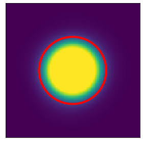
(a) $\epsilon=0.0$

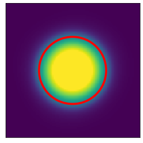
(b) $\epsilon=0.1$

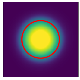
(c) $\epsilon=0.2$

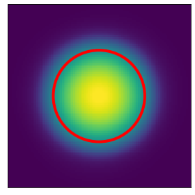
(d) $\epsilon=0.3$

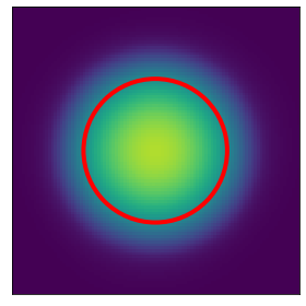
(e) $\epsilon=0.4$

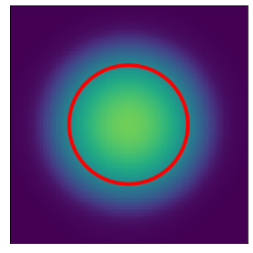
(f) $\epsilon=0.5$

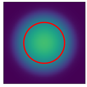
(g) $\epsilon=0.6$

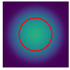
(h) $\epsilon=0.7$

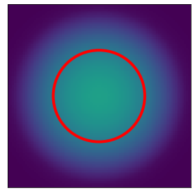
(i) $\epsilon=0.8$

Figure 20: We visualize the Ant’s $x-y$ position visitation heatmaps for different meta-policies towards the end of their training (i.e., in their last $1$ million environment steps, out of $15.2$ million environment steps of training). Here, $\epsilon$ indicates the level of robustness of the meta-policy $\pi_{\theta}^{\epsilon}$. The red circle visualizes the training task distribution for Ant navigation.

Appendix N Cost of learning multiple meta-policies during meta-train phase

Training a population of meta-policies mainly requires more memory (both RAM and GPU) as the meta-policies are trained in parallel. It is true that granularity of epsilon affects the performance of DiAMeTR (as argued in section 4.3). If we increase the number of trained meta-policies, even though DiAMetR’s final performance on various shifted test task distribution would improve, it would take more time/samples for test-time adaptation. While choosing the number of trained meta-policies, we need to balance between final asymptotic performance and time/samples taken for test-time adaptation. The main benefit of learning a distribution of such meta-policies is that it amortizes over many different shifted test time distributions and the meta-policies do not need to be relearned for each of these.

References

- Chen et al. [2022] T. Chen, J. Xu, and P. Agrawal. A system for general in-hand object re-orientation. In A. Faust, D. Hsu, and G. Neumann, editors, Proceedings of the 5th Conference on Robot Learning, volume 164 of Proceedings of Machine Learning Research, pages 297–307. PMLR, 08–11 Nov 2022. URL https://proceedings.mlr.press/v164/chen22a.html.
- Cohen et al. [2019] J. Cohen, E. Rosenfeld, and Z. Kolter. Certified adversarial robustness via randomized smoothing. In International Conference on Machine Learning, pages 1310–1320. PMLR, 2019.
- Collins et al. [2020] L. Collins, A. Mokhtari, and S. Shakkottai. Distribution-agnostic model-agnostic meta-learning. CoRR, abs/2002.04766, 2020. URL https://arxiv.org/abs/2002.04766.
- De Boer et al. [2005] P.-T. De Boer, D. P. Kroese, S. Mannor, and R. Y. Rubinstein. A tutorial on the cross-entropy method. Annals of operations research, 134(1):19–67, 2005.
- Deleu and Bengio [2018] T. Deleu and Y. Bengio. The effects of negative adaptation in model-agnostic meta-learning. arXiv preprint arXiv:1812.02159, 2018.
- Dorfman et al. [2020] R. Dorfman, I. Shenfeld, and A. Tamar. Offline meta learning of exploration. arXiv preprint arXiv:2008.02598, 2020.
- Duan et al. [2016] Y. Duan, J. Schulman, X. Chen, P. L. Bartlett, I. Sutskever, and P. Abbeel. Rl2: Fast reinforcement learning via slow reinforcement learning. arXiv preprint arXiv:1611.02779, 2016.
- Fallah et al. [2021] A. Fallah, A. Mokhtari, and A. Ozdaglar. Generalization of model-agnostic meta-learning algorithms: Recurring and unseen tasks. Advances in Neural Information Processing Systems, 34, 2021.
- Filos et al. [2020] A. Filos, P. Tigkas, R. McAllister, N. Rhinehart, S. Levine, and Y. Gal. Can autonomous vehicles identify, recover from, and adapt to distribution shifts? In International Conference on Machine Learning, pages 3145–3153. PMLR, 2020.
- Finn et al. [2017] C. Finn, P. Abbeel, and S. Levine. Model-agnostic meta-learning for fast adaptation of deep networks. In International conference on machine learning, pages 1126–1135. PMLR, 2017.
- Fu et al. [2021] H. Fu, H. Tang, J. Hao, C. Chen, X. Feng, D. Li, and W. Liu. Towards effective context for meta-reinforcement learning: an approach based on contrastive learning. In Proceedings of the AAAI Conference on Artificial Intelligence, volume 35, pages 7457–7465, 2021.
- Gupta et al. [2018a] A. Gupta, B. Eysenbach, C. Finn, and S. Levine. Unsupervised meta-learning for reinforcement learning. arXiv preprint arXiv:1806.04640, 2018a.
- Gupta et al. [2018b] A. Gupta, R. Mendonca, Y. Liu, P. Abbeel, and S. Levine. Meta-reinforcement learning of structured exploration strategies. Advances in neural information processing systems, 31, 2018b.
- Haarnoja et al. [2018] T. Haarnoja, A. Zhou, P. Abbeel, and S. Levine. Soft actor-critic: Off-policy maximum entropy deep reinforcement learning with a stochastic actor. arXiv preprint arXiv:1801.01290, 2018.
- Hong et al. [2021] J. Hong, H. Wang, Z. Wang, and J. Zhou. Federated robustness propagation: Sharing adversarial robustness in federated learning. arXiv preprint arXiv:2106.10196, 2021.
- Jabri et al. [2019] A. Jabri, K. Hsu, A. Gupta, B. Eysenbach, S. Levine, and C. Finn. Unsupervised curricula for visual meta-reinforcement learning. Advances in Neural Information Processing Systems, 32, 2019.
- Ke et al. [2021] L. Ke, J. Wang, T. Bhattacharjee, B. Boots, and S. Srinivasa. Grasping with chopsticks: Combating covariate shift in model-free imitation learning for fine manipulation. In 2021 IEEE International Conference on Robotics and Automation (ICRA), pages 6185–6191. IEEE, 2021.
- Kumar et al. [2021] A. Kumar, Z. Fu, D. Pathak, and J. Malik. Rma: Rapid motor adaptation for legged robots. arXiv preprint arXiv:2107.04034, 2021.
- Lee et al. [2019] L. Lee, B. Eysenbach, E. Parisotto, E. P. Xing, S. Levine, and R. Salakhutdinov. Efficient exploration via state marginal matching. CoRR, abs/1906.05274, 2019. URL http://arxiv.org/abs/1906.05274.
- Lin et al. [2020] Z. Lin, G. Thomas, G. Yang, and T. Ma. Model-based adversarial meta-reinforcement learning. In H. Larochelle, M. Ranzato, R. Hadsell, M. Balcan, and H. Lin, editors, Advances in Neural Information Processing Systems 33: Annual Conference on Neural Information Processing Systems 2020, NeurIPS 2020, December 6-12, 2020, virtual, 2020. URL https://proceedings.neurips.cc/paper/2020/hash/73634c1dcbe056c1f7dcf5969da406c8-Abstract.html.
- Madry et al. [2017] A. Madry, A. Makelov, L. Schmidt, D. Tsipras, and A. Vladu. Towards deep learning models resistant to adversarial attacks. arXiv preprint arXiv:1706.06083, 2017.
- Margolis et al. [2022] G. B. Margolis, G. Yang, K. Paigwar, T. Chen, and P. Agrawal. Rapid locomotion via reinforcement learning. arXiv preprint arXiv:2205.02824, 2022.
- Mendonca et al. [2020] R. Mendonca, X. Geng, C. Finn, and S. Levine. Meta-reinforcement learning robust to distributional shift via model identification and experience relabeling. CoRR, abs/2006.07178, 2020. URL https://arxiv.org/abs/2006.07178.
- Miki et al. [2022] T. Miki, J. Lee, J. Hwangbo, L. Wellhausen, V. Koltun, and M. Hutter. Learning robust perceptive locomotion for quadrupedal robots in the wild. Science Robotics, 7(62):eabk2822, 2022.
- Mishra et al. [2017] N. Mishra, M. Rohaninejad, X. Chen, and P. Abbeel. A simple neural attentive meta-learner. arXiv preprint arXiv:1707.03141, 2017.
- Mitchell et al. [2021] E. Mitchell, R. Rafailov, X. B. Peng, S. Levine, and C. Finn. Offline meta-reinforcement learning with advantage weighting. In International Conference on Machine Learning, pages 7780–7791. PMLR, 2021.
- Nagabandi et al. [2018] A. Nagabandi, I. Clavera, S. Liu, R. S. Fearing, P. Abbeel, S. Levine, and C. Finn. Learning to adapt in dynamic, real-world environments through meta-reinforcement learning. arXiv preprint arXiv:1803.11347, 2018.
- Nair et al. [2020] A. Nair, A. Gupta, M. Dalal, and S. Levine. Awac: Accelerating online reinforcement learning with offline datasets. arXiv preprint arXiv:2006.09359, 2020.
- Nesterov [2009] Y. Nesterov. Primal-dual subgradient methods for convex problems. Mathematical programming, 120(1):221–259, 2009.
- Ni et al. [2022] T. Ni, B. Eysenbach, S. Levine, and R. Salakhutdinov. Recurrent model-free RL is a strong baseline for many POMDPs, 2022. URL https://openreview.net/forum?id=E0zOKxQsZhN.
- Oikarinen et al. [2021] T. P. Oikarinen, W. Zhang, A. Megretski, L. Daniel, and T. Weng. Robust deep reinforcement learning through adversarial loss. In M. Ranzato, A. Beygelzimer, Y. N. Dauphin, P. Liang, and J. W. Vaughan, editors, Advances in Neural Information Processing Systems 34: Annual Conference on Neural Information Processing Systems 2021, NeurIPS 2021, December 6-14, 2021, virtual, pages 26156–26167, 2021. URL https://proceedings.neurips.cc/paper/2021/hash/dbb422937d7ff56e049d61da730b3e11-Abstract.html.
- Pinto et al. [2017] L. Pinto, J. Davidson, R. Sukthankar, and A. Gupta. Robust adversarial reinforcement learning. In D. Precup and Y. W. Teh, editors, Proceedings of the 34th International Conference on Machine Learning, ICML 2017, Sydney, NSW, Australia, 6-11 August 2017, volume 70 of Proceedings of Machine Learning Research, pages 2817–2826. PMLR, 2017. URL http://proceedings.mlr.press/v70/pinto17a.html.
- Rakelly et al. [2019] K. Rakelly, A. Zhou, C. Finn, S. Levine, and D. Quillen. Efficient off-policy meta-reinforcement learning via probabilistic context variables. In International conference on machine learning, pages 5331–5340. PMLR, 2019.
- Rényi [1961] A. Rényi. On measures of entropy and information. In Proceedings of the Fourth Berkeley Symposium on Mathematical Statistics and Probability, Volume 1: Contributions to the Theory of Statistics, volume 4, pages 547–562. University of California Press, 1961.
- Rothfuss et al. [2018] J. Rothfuss, D. Lee, I. Clavera, T. Asfour, and P. Abbeel. Promp: Proximal meta-policy search. arXiv preprint arXiv:1810.06784, 2018.
- Schulman et al. [2017] J. Schulman, F. Wolski, P. Dhariwal, A. Radford, and O. Klimov. Proximal policy optimization algorithms. CoRR, abs/1707.06347, 2017. URL http://dblp.uni-trier.de/db/journals/corr/corr1707.html#SchulmanWDRK17.
- Sinha et al. [2017] A. Sinha, H. Namkoong, R. Volpi, and J. Duchi. Certifying some distributional robustness with principled adversarial training. arXiv preprint arXiv:1710.10571, 2017.
- Sutton et al. [1999] R. S. Sutton, D. McAllester, S. Singh, and Y. Mansour. Policy gradient methods for reinforcement learning with function approximation. Advances in neural information processing systems, 12, 1999.
- Thrun and Pratt [1998] S. Thrun and L. Y. Pratt, editors. Learning to Learn. Springer, 1998. ISBN 978-1-4613-7527-2. doi: 10.1007/978-1-4615-5529-2. URL https://doi.org/10.1007/978-1-4615-5529-2.
- Vaserstein [1969] L. N. Vaserstein. Markov processes over denumerable products of spaces, describing large systems of automata. Problemy Peredachi Informatsii, 5(3):64–72, 1969.
- Vinitsky et al. [2020] E. Vinitsky, Y. Du, K. Parvate, K. Jang, P. Abbeel, and A. M. Bayen. Robust reinforcement learning using adversarial populations. CoRR, abs/2008.01825, 2020. URL https://arxiv.org/abs/2008.01825.
- Wolpert and Macready [1997] D. Wolpert and W. Macready. No free lunch theorems for optimization. IEEE Transactions on Evolutionary Computation, 1(1):67–82, 1997. doi: 10.1109/4235.585893.
- Wu et al. [2021] M. Wu, N. Goodman, C. Piech, and C. Finn. Prototransformer: A meta-learning approach to providing student feedback. arXiv preprint arXiv:2107.14035, 2021.
- Xie et al. [2022] A. Xie, S. Sodhani, C. Finn, J. Pineau, and A. Zhang. Robust policy learning over multiple uncertainty sets. arXiv preprint arXiv:2202.07013, 2022.
- Zhang et al. [2021a] H. Zhang, H. Chen, D. S. Boning, and C. Hsieh. Robust reinforcement learning on state observations with learned optimal adversary. In 9th International Conference on Learning Representations, ICLR 2021, Virtual Event, Austria, May 3-7, 2021. OpenReview.net, 2021a. URL https://openreview.net/forum?id=sCZbhBvqQaU.
- Zhang et al. [2021b] J. Zhang, J. Wang, H. Hu, T. Chen, Y. Chen, C. Fan, and C. Zhang. Metacure: Meta reinforcement learning with empowerment-driven exploration. In International Conference on Machine Learning, pages 12600–12610. PMLR, 2021b.
- Zhao et al. [2020] T. Z. Zhao, A. Nagabandi, K. Rakelly, C. Finn, and S. Levine. Meld: Meta-reinforcement learning from images via latent state models. arXiv preprint arXiv:2010.13957, 2020.
- Zintgraf et al. [2019] L. Zintgraf, K. Shiarlis, M. Igl, S. Schulze, Y. Gal, K. Hofmann, and S. Whiteson. Varibad: A very good method for bayes-adaptive deep rl via meta-learning. arXiv preprint arXiv:1910.08348, 2019.
- Zintgraf et al. [2021] L. M. Zintgraf, L. Feng, C. Lu, M. Igl, K. Hartikainen, K. Hofmann, and S. Whiteson. Exploration in approximate hyper-state space for meta reinforcement learning. In International Conference on Machine Learning, pages 12991–13001. PMLR, 2021.