Adaptive Ranking-based Sample Selection
for Weakly Supervised Class-imbalanced Text Classification

Abstract

To obtain a large amount of training labels inexpensively, researchers have recently adopted the weak supervision (WS) paradigm, which leverages labeling rules to synthesize training labels rather than using individual annotations to achieve competitive results for natural language processing (NLP) tasks. However, data imbalance is often overlooked in applying the WS paradigm, despite being a common issue in a variety of NLP tasks. To address this challenge, we propose Adaptive Ranking-based Sample Selection (ARS2), a model-agnostic framework to alleviate the data imbalance issue in the WS paradigm. Specifically, it calculates a probabilistic margin score based on the output of the current model to measure and rank the cleanliness of each data point. Then, the ranked data are sampled based on both class-wise and rule-aware ranking. In particular, the two sample strategies corresponds to our motivations: (1) to train the model with balanced data batches to reduce the data imbalance issue and (2) to exploit the expertise of each labeling rule for collecting clean samples. Experiments on four text classification datasets with four different imbalance ratios show that ARS2 outperformed the state-of-the-art imbalanced learning and WS methods, leading to a 2%-57.8% improvement on their F1-score. Our implementation can be found in https://github.com/JieyuZ2/wrench/blob/main/wrench/endmodel/ars2.py.

1 Introduction

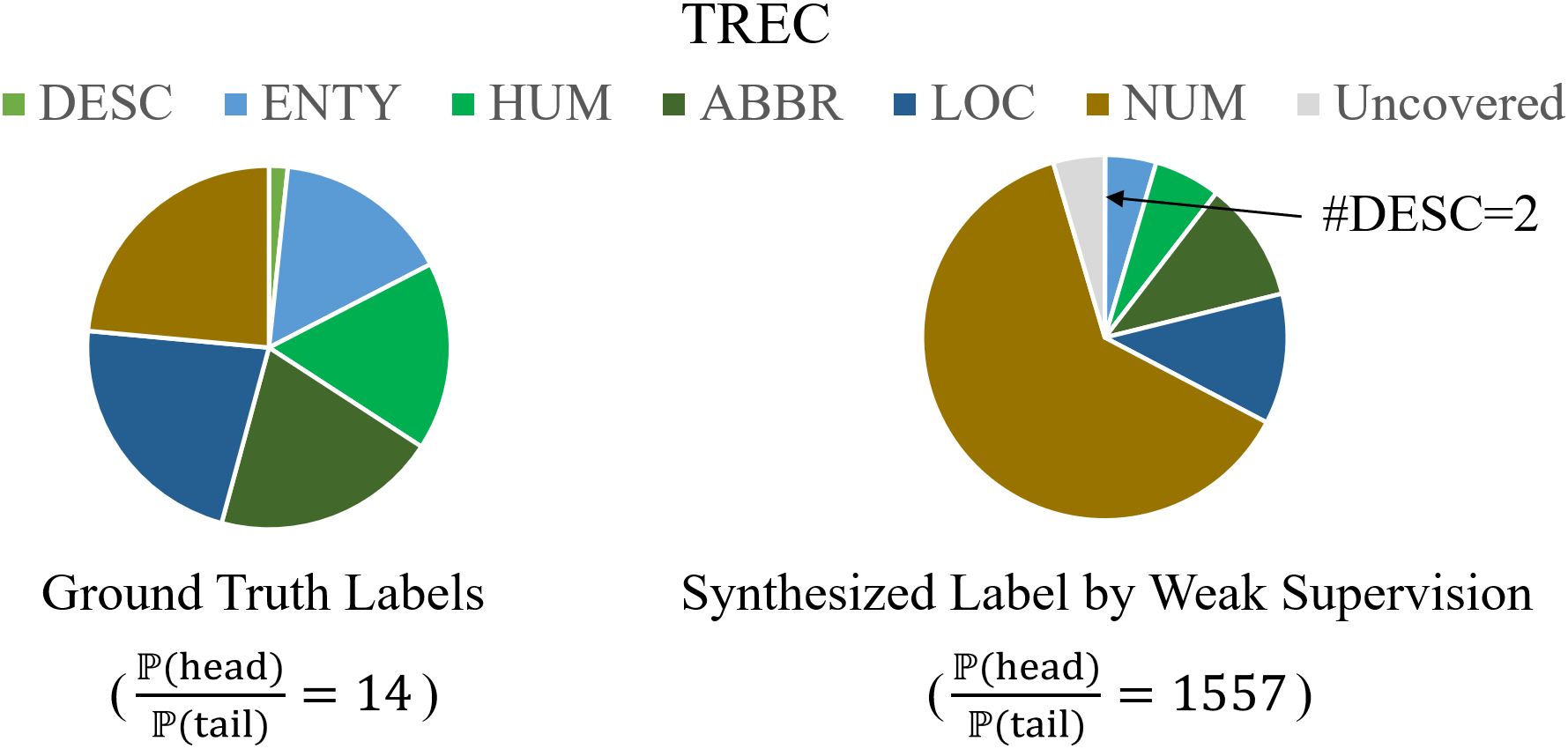
Figure 1: Comparison of class distribution between the ground truth labels and labels produced by weak supervision (WS) on TREC dataset. The uncovered piece represents the data not covered by any labeling rule in WS. It may be observed that WS amplified the class imbalance.

Deep learning models rely heavily on high-quality yet expensive, labeled data. Owing to this considerable cost, the weak supervision (WS) paradigm has increasingly been used to reduce human efforts Ratner et al. (2016a); Zhang et al. (2021). This approach synthesizes training labels with labeling rules to significantly improve the efficiency of creating training sets and have achieved competitive results in natural language processing (NLP) Yu et al. (2020); Ren et al. (2020); Rühling Cachay et al. (2021). However, existing methods leveraging the WS paradigm to perform NLP tasks mostly focus on reducing the noise in training labels brought by labeling rules, while ignoring the common and critical problem of data imbalance. In fact, in a preliminary experiment performed as part of the present work (Fig. 1), we found that the WS paradigm may amplify the imbalance ratio of the dataset because the synthesized training labels tend to have more imbalanced distribution.

To address this issue, we propose ARS2 as a general model-agnostic framework based on the WS paradigm. ARS2 is mainly divided in two steps, including (1) warm-up, in which stage noisy data is used to train the model and obtain a noise detector; (2) continual training with adaptive ranking-based sample selection. In this stage, we use the noise detector trained in the warm-up stage to evaluate the cleanliness of the data, and use the ranking obtained based on this evaluation to sample the data. We followed previous works Ratner et al. (2016a); Ren et al. (2020); Zhang et al. (2022b) in using heuristic programmatic rules to annotate the data. In weak supervised learning, researchers use a label model to aggregate weak labels annotated by rules to estimate the probabilistic class distribution of each data point. In this work, we use a label model to integrate the weak labels given by the rules as pseudo-labels during the training process to obviate the need for manual labeling.

To select the samples most likely to be clean, we adopt a selection strategy based on small-loss, which is a very common method that has been verified to be effective in many situations Jiang et al. (2018); Yu et al. (2019); Yao et al. (2020). Specifically, deep neural networks, have strong ability of memorization Wu et al. (2018); Wei et al. (2021), will first memorize labels of clean data and then those of noisy data with the assumption that the clean data are of the majority in a noisy dataset. Data with small loss can thus be regarded as clean examples with high probability. Inspired by this approach, we propose probabilistic margin score (PMS) as a criterion to judge whether data are clean. Instead of using the confidence given by a model directly, a confidence margin is used for better performance Ye et al. (2020). We also performed a comparative experiment on the use of margin versus the direct use of confidence, as described in Sec. 3.3.

Sample selection based on weak labels can lead to severe class imbalance. Consequently, models trained using these imbalanced subsets can exhibit both superior performance on majority classes and inferior performance on minority classes Cui et al. (2019). A reweighted loss function can partially address this problem. However, performance remains nonetheless limited by noisy labels, that is, data with majority-class features may be annotated as minority-class data incorrectly, which misleads the training process. Therefore, we propose a sample selection strategy based on class-wise ranking (CR) to address imbalanced data. Using this strategy, we can select relatively balanced sample batches for training and avoid the strong influence of the majority class.

To further exploit the expertise of labeling rules, we also propose another sample selection strategy called rule-aware ranking (RR). We use aggregated labels as pseudo-labels in the WS paradigm and discards weak labels. However, the annotations generated by rules are likely to contain a considerable amount of valid information. For example, some rules yield a high proportion of correct results. The higher the PMS, the more likely the labeling result of the rules is to be close to the ground truth. Using this strategy, we can select batches with clean data for training and avoid the influence of noise.

The primary contributions of this work are summarized as follows. (1) We propose a general, model-agnostic weakly supervised leading framework called ARS2 for imbalanced datasets; (2) we also propose two reliable adaptive sampling strategies to address data imbalance issues. (3) The results of experiments on four benchmark datasets are presented to demonstrate that the ARS2 improved on the performance of existing imbalanced learning and weakly supervised learning methods, by 2%-57.8% in terms of F1-score.

2 Weakly Supervised Class-imbalanced Text Classification

2.1 Problem Formulation

In this work, we study class-imbalanced text classification in a setting with weak supervision. Specifically, we consider an unlabeled dataset $\mathcal{D}$ consisting of $N$ documents, each of which is denoted by $x_{i}\in\mathcal{X}$. For each document $x_{i}$, the corresponding label $y_{i}\in\mathcal{Y}=\{1,2,...,C\}$ is unknown to us, whereas the class prior $p(y)$ is given and highly imbalanced. Our goal is to learn a parameterized function $f(\cdot;\bm{\theta}):\mathcal{X}\xrightarrow{}\Delta^{C}$ which outputs the class probability $p(y\mid x)$ and can be used to classify documents during inference.

To address the lack of ground truth training labels, we adopt the two-stage weak supervision paradigm Ratner et al. (2016b); Zhang et al. (2021). In particular, we rely on $k$ user-provided heuristic rules $\{r_{i}\}_{i\in\{1,...,k\}}$ to provide weak labels. Each rule $r_{i}$ is associated with a particular label $y_{r_{i}}\in\mathcal{Y}$, and we denote by $l_{i}$ the output of the rule $r_{i}$. It either assigns the associated label ($l_{i}=y_{r_{i}}$) to a given document or abstains ($l_{i}=-1$) on this example. Note that the user-provided rules could be noisy and conflict with one another. For the document $x$, we concatenate the output weak labels of $k$ rules $l_{1},...,l_{k}$ as $\bm{l}_{x}$. Throughout this work, we apply the weak labels output by heuristic rules to train a text classifier.

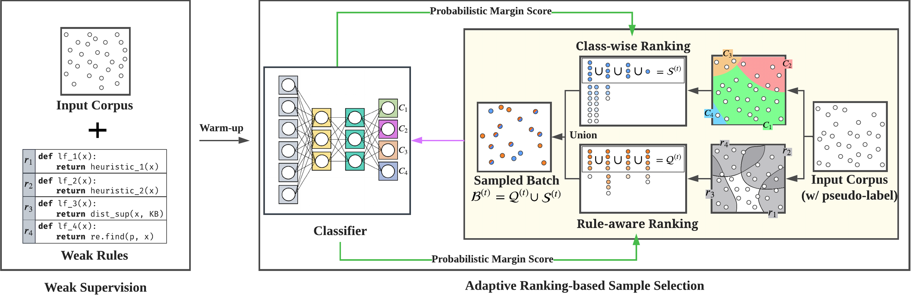
Figure 2: Overview of ARS2. Our framework has two stages: (1) warm-up, which is used to let the model learn how to distinguish noisy data; (2) continual training with adaptive sampling, which is used to sample clean data. We adopt two different adaptive sampling strategies, including class-wise ranking sampling and rule-aware ranking sampling.

2.2 Aggregation of Weak Labels

Label models are used to aggregate weak labels under the weak supervision paradigm, which are in turn used to train the desired end model in the next stage. Existing label models include Majority Voting (MV), Probabilistic Graphical Models (PGM) Dawid and Skene (1979); Ratner et al. (2019b); Fu et al. (2020), etc. In this research, we use PGM implement by Ratner et al. (2019b) as our label model $g(\cdot)$, which can be described as

$$g(\bm{l}_{x})=\mathbb{P}(y\mid\bm{l}_{x}).$$ (1)

This assumes that $\bm{l}_{x}$ as a random variable for label model. After modeling the relationship between the observed variable $\bm{l}_{x}$ and unobserved variable $y$ by Bayes methods, the label model obtains the posterior distribution of $y$ given $\bm{l}_{x}$ by inference process like expectation maximization or variational inference. Finally, we set the maximum value of $\mathbb{P}(y\mid\bm{l}_{x})$ as the hard pseudo-label $\tilde{y}_{x}$ of $x$ for later end model training.

2.3 Adaptive Ranking-based Sample Selection

We propose an adaptive ranking sample selection approach to simultaneously solve the problems caused by data imbalance and those resulting from the noise generated by the application of procedural rules. First, the classification model $f(\cdot;\bm{\theta})$ is warmed up with pseudo-labels $\tilde{y}_{x}$, which are used to train the model as a noise indicator that can discriminate noise in the next stage. Then, we continue training the warmed-up model by using the data sampled by adaptive data sampling strategies, including class-wise ranking (CR) and rule-aware ranking (RR) supported by probabilistic margin score (PMS). The training procedures are summarized in Algorithm 1 and the proposed framework is illustrated in Figure 2.

Input: Weak labeled training data $\mathcal{X}$; Pseudo label $\tilde{y}$; Classification model $f(\cdot;\bm{\theta})$.

// Warm-up $f(\cdot,\bm{\theta})$ with weak labeled data.

for $t=1,2,\cdots,T$ do

       1. Sample a minibatch $\mathcal{B}$ from $\mathcal{X}$.

       2. Update $\theta$ by Eq. (2) before early stop.

// Continue training with sample selection.

for $t=1,2,\cdots,T_{s}$ do

       1. Calculate score for all $x\in\mathcal{X}$ (Sec. 2.4).

       2. Sample $\mathcal{Q}^{(t)}$ from $\mathcal{X}$ (Sec. 2.5).

       3. Sample $\mathcal{S}^{(t)}$ from $\mathcal{X}$ (Sec. 2.6).

       4. Update $\theta$ using $\mathcal{U}^{(t)}=\mathcal{Q}^{(t)}\cup\mathcal{S}^{(t)}$ by Eq. (3).

Output: Output final model $f(\cdot;\bm{\theta})$.

Algorithm 1 ARS2

Warm-up.

Inspired by Zheng et al. (2020), the prediction of a noisy classification model can be a good indicator of whether the label of a training data point is clean. Our method relies on a noise indicator trained at warm-up to determine whether each training data is clean. However, a model with sufficient capacity (e.g., more parameters than training examples) can “memorize” each example, overfitting the training set and yielding poor generalization to validation and test sets Goodfellow et al. (2016). To prevent a model from overfitting noisy data, we warm-up the model $f(\cdot;\bm{\theta})$ with early stopping Dodge et al. (2020), and solve the optimization problem by

$$\min_{\bm{\theta}}\frac{1}{N}\sum_{x\in\mathcal{X}}\mathcal{L}(f(x;\bm{\theta}),\tilde{y}_{x}),$$ (2)

where $\mathcal{L}$ denotes a loss function and $\tilde{y}_{x}$ is pseudo-label aggregated by a label model. In this research, we do not limit the definition of the loss function; that is, any loss function suitable for a multi-classification task can be used.

Continual training with sample selection.

Noisy and imbalanced labels impair the predictive performance of learning models, especially deep neural networks, which tend to exhibit a strong memorization capability Wu et al. (2018); Wei et al. (2021). To reduce the influence of imbalance and noise in the classification model, we adopt the intuitive approach of simply continuing the training process with clean and balanced data. In the continual training phase, we filter for clean data filter using a warmed-up model and sample data in a balanced way to calibrate the model. This procedure provides a more robust performance on a noisy, imbalanced dataset. To achieve this, we propose a measurement of label quality called probabilistic margin score (PMS) (Sec. 2.4), using two sample selection strategies, including class-wise ranking (CR) (Sec. 2.5) and rule-aware ranking (RR) (Sec. 2.6). We adopt batch sampling by using CR as $\mathcal{S}$ and RR as $\mathcal{Q}$ after several steps, using batch $\mathcal{U}=\mathcal{Q}\cup\mathcal{S}$ to continue training the model by solving the following optimization problem.

$$\min_{\bm{\theta}}\frac{1}{|\mathcal{U}|}\sum_{x\in\mathcal{U}}\mathcal{L}(f(x;\bm{\theta}),\tilde{y}_{x}).$$ (3)

Dynamic-Rate Sampling

During the training procedure, the model learns from data with easy/frequent patterns and those with harder/irregular patterns in separate training stages Arpit et al. (2017). According to Chen et al. (2020), a small amount of clean data should be selected first, and then a larger amount of clean data can be selected after the model has been trained well. Therefore, instead of fixing the number of selected data, as the continual training stage proceeds, we linearly increase the size of the training batch $\mathcal{U}$ by

$$k=\frac{B}{C}\times(1+\frac{t(\gamma-1)}{T_{s}}),$$ (4)

where $B$ indicates batch size. The sampling ratio $\gamma$ ranged from 1 to 10 in our experiments.

2.4 Probabilistic Margin Score

To measure the impact of the training label on label quality, inspired by Pleiss et al. (2020), we use the margin of output predictions to identify data with low label quality for later adaptive ranking-based sample selection. The predictions of the network can be regarded as a measurement of the quality of labels, which means that a correct prediction indicates high label quality, and vice versa Jiang et al. (2018); Yu et al. (2019); Yao et al. (2020). Moreover, margins are advantageous because they are simple and efficient to compute during training, and they naturally factorize across samples, which makes it possible to estimate the contribution of each data point to label quality.

Base on this idea, we propose the probabilistic margin score (PMS) to reflect the quality of a given label. PMS is formulated as

$$s(x)=f_{\tilde{y}}(x;\bm{\theta})-\underset{y\in\mathcal{Y}\setminus\{\tilde{y}\}}{\text{max}}f_{y}(x;\bm{\theta}),$$ (5)

where $f_{y}(\cdot;\bm{\theta})$ denotes the prediction of $y$ by classification model $f(\cdot;\bm{\theta})$ and $s(x)\in[-1,1]$. A negative margin corresponds to an incorrect prediction, and vice versa. The margin captures how much lager the (potentially incorrect) assigned confidence is than all other confidences, which indicates the label quality of $x$.

2.5 Class-wise Ranking

If the top-ranked data are directly selected based on PMS to form the training batch, the majority-class data are highly like to dominate the selected batch. This class imbalance in the data results in suboptimal performance. To overcome this problem, we propose class-wise ranking (CR). Specifically, instead of naively selecting the top-k data ranked by PMS from the entire training set, we select top-ranked data from each class to maintain the class balance of the resultant batch. However, CR might introduce more noise if we attempted to construct a perfectly class-balanced data batch. Thus, to reduce the noise while ensuring class balance as much as possible, we set a threshold on PMS to filter the noisy data.

We assume that the set of data belonging to class $y_{i}$ is $\mathcal{X}_{y_{i}}$ and extract the top-k ranked data from each $\mathcal{X}_{y_{i}}$ as $\mathcal{S}^{(t)}_{y_{i}}$ at step $t$ according to the ranking result from $s(\mathcal{X})$. We also set a threshold $\xi$ for $s(\mathcal{X})$ to filter noisy data.

$$\mathcal{S}^{(t)}_{y_{i}}=\underset{x\in\mathcal{X}_{y_{i}},s(x)>\xi}{\text{top-k}}\ s(x).$$ (6)

Then, we concatenate $\mathcal{S}^{(t)}_{y_{i}}$ drawn from each class as a new batch $\mathcal{S}^{(t)}$ as given below.

$$\mathcal{S}^{(t)}=\bigcup_{y_{i}\in\mathcal{Y}}\mathcal{S}^{(t)}_{y_{i}}.$$ (7)

2.6 Rule-aware Ranking

As discussed above, the training labels are synthesized from multiple labeling rules. In the proposed framework, these labeling rules are used not only to produce training labels as in a typical WS pipeline, but also to guide the sample selection. Specifically, each labeling rule typically assigns a certain label, e.g., sports, to only a part of the training set based on its expertise. Within this part of the dataset, some of the data must actually belong to the class sports; otherwise, the relevant labeling rule would be useless. Thus, we propose rule-aware ranking (RR) to separately rank the data covered by each labeling rule and then extract the top-ranked data from each individual ranking. We plan to elaborate on this selection process in a sequel to the present work.

We denote the set of data covered by each labeling rule $r_{i}$ as $\mathcal{X}_{r_{i}}$. We then rank $\mathcal{X}_{r_{i}}$ based on PMS $s(x)$ and extract the top-k data from each $\mathcal{X}_{r_{i}}$ as $\mathcal{Q}^{(t)}_{r_{i}}$ at step $t$.

$$\mathcal{Q}^{(t)}_{r_{i}}=\underset{x\in\mathcal{X}_{r_{i}}}{\text{top-k}}\ s(x).$$ (8)

Specifically, to avoid the error-propagation, we use the weak label $l_{x}$ instead of $\tilde{y}_{x}$ as the new label of $x\in\mathcal{Q}^{(t)}_{r_{i}}$ when $l_{x}$ is unipolar. We claim that data with high confidence will also have a high probability of weak labels being equal to ground truth labels, especially when multiple rules assign the same weak label to the data. The main reason is that those weak labels are not influenced by the training process and are weakly supervised by human level. Then, we take the union of $\mathcal{Q}^{(t)}_{r_{i}}$ drawn from each subset as a new batch $\mathcal{Q}^{(t)}$.

$$\mathcal{Q}^{(t)}=\bigcup_{r_{i}\in\bm{r}}\mathcal{Q}^{(t)}_{r_{i}}.$$ (9)

3 Experiment

3.1 Experiment Setup

Tasks and Datasets.

To evaluate the proposed methods, we used four open benchmark datasets, including AGNews (news topic classification), Yelp (sentiment classification) Zhang et al. (2015), TREC (question classification Li and Roth (2002)) and ChemProt (relation classification Krallinger et al. (2017)). Specifically, each dataset was weakly annotated by several rules provided by Ren et al. (2020); Awasthi et al. (2020); Yu et al. (2020). The relevant statistic for each dataset are shown in Table 1.

Dataset Task # Class # Rule # Train # Valid # Test AG News News Topic Class. 4 9 96k 12k 12k Yelp Sentiment Class. 2 8 30.4k 3.8k 3.8k TREC Question Class. 6 68 4.9k 500 500 ChemProt Relation Class. 10 26 12.8k 1.6k 1.6k

Table 1: Dataset Statistics.

Imbalance Learning Setups.

Following Cui et al. (2019), we created an imbalanced version of AGNews and Yelp by reducing the training and validation examples for each class with an exponential function according to the ground truth data labels. We set four different imbalance ratios $\rho=\max_{y}\mathbb{P}(x)/\min_{y}\mathbb{P}(x)$ for AGNews and Yelp in 1, 10, 20 and 50, respectively. We used the original versions of TREC and Chemprot, as they are known to be imbalanced. Relevant statistics on the imbalanced datasets are shown in A.1.

Weak Supervision Setups.

In weak supervision, assume that the data is not artificially annotated, the labels are annotated by a label model instead of using the ground truth labels. The label model can analyze the results of rule-based annotation and output the most likely label for a given data sample. Throughout the experiments, we used Snorkel Ratner et al. (2019b) as the label model to aggregate the outputs of labeling rules.

	Agnews (Imbalance Ratio ($\downarrow$))				Yelp (Imbalance Ratio ($\downarrow$))				TREC	Chemprot
Method ($\downarrow$)	1	10	20	50	1	10	20	50	-	-
CE+LA	$0.854\pm 0.001$	$0.843\pm 0.005$	$0.826\pm 0.010$	$0.753\pm 0.037$	$0.914\pm 0.003$	$0.877\pm 0.016$	$0.694\pm 0.097$	$0.515\pm 0.145$	$0.394\pm 0.033$	$0.340\pm 0.004$
CE+EN	$0.857\pm 0.003$	$0.834\pm 0.007$	$0.824\pm 0.005$	$0.772\pm 0.016$	$0.916\pm 0.002$	$0.723\pm 0.200$	$0.806\pm 0.012$	$0.658\pm 0.036$	$0.450\pm 0.005$	$0.389\pm 0.030$
CE+EN+LA	$0.854\pm 0.007$	$0.836\pm 0.005$	$0.838\pm 0.004$	$0.786\pm 0.020$	$0.919\pm 0.002$	$0.610\pm 0.204$	$0.807\pm 0.013$	$0.699\pm 0.023$	$0.409\pm 0.152$	$0.336\pm 0.010$
Dice	$0.855\pm 0.003$	$0.846\pm 0.006$	$0.746\pm 0.003$	$0.590\pm 0.033$	$0.882\pm 0.003$	$0.821\pm 0.048$	$0.637\pm 0.241$	$0.323\pm 0.000$	$0.476\pm 0.022$	$0.233\pm 0.010$
LDAM	$0.804\pm 0.090$	$0.828\pm 0.012$	$0.813\pm 0.009$	$0.100\pm 0.002$	$0.819\pm 0.052$	$0.751\pm 0.042$	$0.388\pm 0.100$	$0.342\pm 0.002$	$0.154\pm 0.033$	$0.356\pm 0.005$
COSINE	0.854 $\pm$ 0.004	0.720 $\pm$ 0.068	0.822 $\pm$ 0.003	0.574 $\pm$ 0.004	0.912 $\pm$ 0.001	0.496 $\pm$ 0.192	0.836 $\pm$ 0.008	0.820 $\pm$ 0.000	0.477 $\pm$ 0.001	0.346 $\pm$ 0.009
Denoise	0.852 $\pm$ 0.001	0.537 $\pm$ 0.111	0.526 $\pm$ 0.112	0.471 $\pm$ 0.188	0.811 $\pm$ 0.004	0.343 $\pm$ 0.004	0.498 $\pm$ 0.126	0.323 $\pm$ 0.000	0.236 $\pm$ 0.021	0.259 $\pm$ 0.075
ARS2 (w/o CR&RR)	0.854 $\pm$ 0.001	0.840 $\pm$ 0.006	0.818 $\pm$ 0.035	0.810 $\pm$ 0.024	0.917 $\pm$ 0.006	0.868 $\pm$ 0.011	0.822 $\pm$ 0.057	0.738 $\pm$ 0.066	0.342 $\pm$ 0.033	0.396 $\pm$ 0.021
ARS2 (w/o RR)	0.854 $\pm$ 0.000	0.840 $\pm$ 0.005	0.797 $\pm$ 0.078	0.777 $\pm$ 0.023	0.920 $\pm$ 0.003	0.844 $\pm$ 0.021	0.764 $\pm$ 0.096	0.794 $\pm$ 0.054	0.348 $\pm$ 0.028	0.402 $\pm$ 0.033
ARS2 (w/o CR)	0.884 $\pm$ 0.006	0.842 $\pm$ 0.005	0.818 $\pm$ 0.022	0.759 $\pm$ 0.069	0.929 $\pm$ 0.002	0.861 $\pm$ 0.031	0.750 $\pm$ 0.132	0.555 $\pm$ 0.165	0.490 $\pm$ 0.065	0.303 $\pm$ 0.004
ARS2 (Conf.)	0.854 $\pm$ 0.001	0.847 $\pm$ 0.006	0.821 $\pm$ 0.015	0.819 $\pm$ 0.018	0.939 $\pm$ 0.001	0.908 $\pm$ 0.004	0.851 $\pm$ 0.028	0.835 $\pm$ 0.034	0.574 $\pm$ 0.027	0.342 $\pm$ 0.003
ARS2	0.882 $\pm$ 0.003	0.859 $\pm$ 0.012	0.844 $\pm$ 0.035	0.827 $\pm$ 0.011	0.936 $\pm$ 0.002	0.910 $\pm$ 0.003	0.852 $\pm$ 0.024	0.854 $\pm$ 0.012	0.597 $\pm$ 0.025	0.404 $\pm$ 0.006

Table 2: F1-macro result on 2-layer MLP. Comparison among imbalance learning methods, weak supervision methods, and ASR2 (as well as its variants). The ranking of using confidence is identical to that ranked by negative loss. Note that ARS2 outperform all baselines in all imbalanced datasets.

Implementation Details.

We choose the Multi-Layer Perceptron (MLP) with 2 hidden layers and RoBERTa Liu et al. (2019) as the backbone language model for our method in all baselines. In the case of using RoBERTa as a backbone model, rather than training the RoBERTa as a noise indicator in warm-up stage, we used a warmed-up MLP as a noisy indicator to sample training batches for RoBERTa because a large model may easily overfit noisy data in a few steps. We used the classification macro-average F1 score on the test set as the evaluation metric for all datasets. We implemented our method using PyTorch Paszke et al. (2019) with the WRENCH code-base Zhang et al. (2021).

3.2 Baselines

Imbalance Learning Methods:

(1) Logit Adjustment (LA) Menon et al. (2020): This method combines post-hoc weight normalization and loss modification to balance head and tail classes by adding a class-wise offset to the loss. (2) Effective Number (EN) Cui et al. (2019): This method uses the proportion of sampled data as the class-wise weight of loss function, which helps the model to learn a useful decision boundary. (3) Dice Loss (Dice) Li et al. (2019): The dice loss method uses dynamically adjusted weight to improve the S$\phi$rensen-Dice coefficient (a method that values both false positive and false negative and works well for imbalanced datasets), which reduces the impact of easy negative data during training. (4) LDAM Cao et al. (2019a): This method encourages the model to treat the optimal trade-off problem between per-class margins. (5) Effective Number + Logit Adjustment: Because the effective number is a class-wise re-weighting method, we have also combined this method with logit adjustment as a baseline.

Weak Supervision Methods:

(1) COSINE Yu et al. (2020) The COSINE method uses weakly labeled data to fine-tune pre-trained language models by contrastive self-training. (2) Denoise Ren et al. (2020): This method estimates the source reliability using a conditional soft attention mechanism and then reducing label noise by aggregating weak labels annotated by a set of rules.

3.3 Main Result

Our main results on a 2-layer MLP model are reported in Table 2. Our method outperformed all the baselines on both balanced and imbalanced datasets. The results of the experiment also indicated the following.

The performance of all baseline methods generally showed a downward trend with increasing imbalance ratio, and the decline was more evident in the binary classification problem of Yelp. In contrast, on the multi-classification problem dataset AGNews, although the head class and the tail class exhibited a relatively large gap because the number of each class declined step-by-step, the ratio between the head class and the second head class did not reach the value of the imbalance ratio. Therefore, the model’s performance decline on multi-classification was slightly smaller than in binary classification.

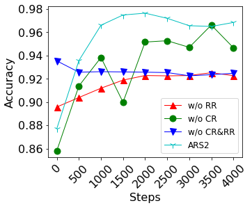
(a) $\rho=10$

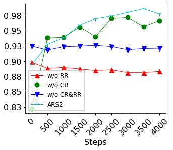
(b) $\rho=20$

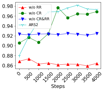
(c) $\rho=50$

Figure 3: The quality of the selected data in AGNews under each imbalance ratio.

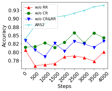
(a) $\rho=10$

(b) $\rho=20$

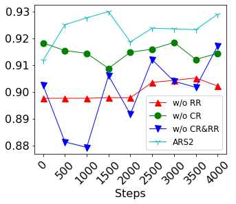
(c) $\rho=50$

Figure 4: The quality of the selected data in Yelp under each imbalance ratio.

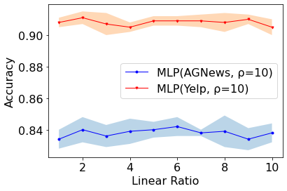
(a) Linear Ratio

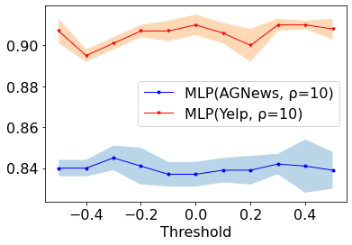
(b) Threshold

Figure 5: Hyperparameter Study

On the balanced dataset, the performance of ARS2 was very similar to that of using RR only, whereas the performance of ARS2 (w/o CR) was slightly better than that of ARS2 in AGNews. This occurred because CR did not operate as intended on the balanced dataset but instead affected the diversity of data, resulting in a small gap between ARS2 and RR on the balanced set. The role of CR became gradually more prominent with increasing imbalance ratio because CR was able to balance the original unbalanced sample set such that the model was not affected by the data from the majority class, improving performance.

The baseline performance gradually weakened with the increase in the imbalance ratio. These baselines were all loss-modification-related methods. In the noisy dataset, if a data point originally belonging to the head class is incorrectly marked as belonging to a tail class, the loss modification feature causes the model to assign a larger weight to the data that may have noise, which deepens the error of the model, and results in poor training performance.

3.4 Ablation Study

We also examined the importance of CR, RR, and different measurements of label quality. The 8th, 9th and 11th rows of Table 2 summarize the results. It may be observed that the performance of ARS2 without CR on the balanced set was almost the same as that of ARS2, which shows that RR was the main contributor to the balanced set. However, the contributions of both start to converge with increasing imbalance ratio. This shows that the data filtered by CR can allow the model to learn more balance features from the imbalance dataset, whereas RR can make the process smoother and reduce the model’s misjudgment of high-ranking data.

We also compared the performance of two ranking scores. The 11th and 12th rows of Table 2 show that ARS2 with PMS performed better than with confidence, except for the Yelp dataset with an imbalance ratio of $1$. However, the difference in performance in this situation was less than 1%. This shows that PMS can reflect the cleanliness of data better, and thus may be considered a more useful ranking score.

3.5 Hyperparameter Study

We studied two hyperparameters, namely $\gamma$ and $\xi$ used in controlling the quality of adaptive sampling. We set the linear ratio from $1$ to $10$, where higher values of the linear ratio indicate larger amounts of data in the sampled batch. We also set the threshold from -0.5 to 0.5, which indicated the quality of the data of our sampled batch. Figures 5(a) shows that ARS2 is insensitive to $\gamma$ as the performance is less than 0.8%. In the case of Yelp, ARS2 cannot perform well with a small threshold (less than 0) because the loose threshold may lead a large amount of noisy data to affect the training process. While in the case of AGNews, the high quality of rules helps RR to re-corrected the noisy label, increase the clean data points accessed by model during training.

	AGNews (Imbalance Ratio ($\downarrow$))				Yelp (Imbalance Ratio ($\downarrow$))				TREC	Chemprot
Method ($\downarrow$)	1	10	20	50	1	10	20	50	-	-
CE+LA	0.858 $\pm$ 0.002	0.847 $\pm$ 0.004	0.833 $\pm$ 0.009	0.823 $\pm$ 0.030	0.949 $\pm$ 0.005	0.900 $\pm$ 0.014	0.837 $\pm$ 0.103	0.323 $\pm$ 0.000	0.545 $\pm$ 0.014	0.349 $\pm$ 0.019
CE+EN	0.859 $\pm$ 0.002	0.841 $\pm$ 0.005	0.852 $\pm$ 0.006	0.823 $\pm$ 0.020	0.941 $\pm$ 0.014	0.897 $\pm$ 0.026	0.653 $\pm$ 0.270	0.323 $\pm$ 0.000	0.561 $\pm$ 0.022	0.453 $\pm$ 0.004
CE+EN+LA	0.861 $\pm$ 0.001	0.851 $\pm$ 0.004	0.838 $\pm$ 0.007	0.809 $\pm$ 0.051	0.947 $\pm$ 0.002	0.882 $\pm$ 0.058	0.839 $\pm$ 0.076	0.323 $\pm$ 0.000	0.505 $\pm$ 0.068	0.039 $\pm$ 0.018
Dice	0.874 $\pm$ 0.001	0.875 $\pm$ 0.002	0.865 $\pm$ 0.005	0.800 $\pm$ 0.064	0.939 $\pm$ 0.007	0.628 $\pm$ 0.267	0.848 $\pm$ 0.102	0.323 $\pm$ 0.000	0.455 $\pm$ 0.029	0.064 $\pm$ 0.008
LDAM	0.859 $\pm$ 0.002	0.823 $\pm$ 0.007	0.815 $\pm$ 0.004	0.836 $\pm$ 0.009	0.943 $\pm$ 0.008	0.828 $\pm$ 0.025	0.350 $\pm$ 0.035	0.323 $\pm$ 0.000	0.479 $\pm$ 0.019	0.121 $\pm$ 0.060
COSINE	0.874 $\pm$ 0.003	0.852 $\pm$ 0.013	0.836 $\pm$ 0.015	0.825 $\pm$ 0.012	0.884 $\pm$ 0.048	0.323 $\pm$ 0.000	0.804 $\pm$ 0.033	0.329 $\pm$ 0.007	0.619 $\pm$ 0.024	0.385 $\pm$ 0.002
Denoise	0.868 $\pm$ 0.003	0.202 $\pm$ 0.002	0.363 $\pm$ 0.243	0.246 $\pm$ 0.096	0.954 $\pm$ 0.002	0.559 $\pm$ 0.037	0.323 $\pm$ 0.000	0.323 $\pm$ 0.000	0.473 $\pm$ 0.015	0.066 $\pm$ 0.015
ARS2	0.893 $\pm$ 0.007	0.890 $\pm$ 0.011	0.868 $\pm$ 0.026	0.851 $\pm$ 0.024	0.954 $\pm$ 0.004	0.956 $\pm$ 0.005	0.955 $\pm$ 0.007	0.910 $\pm$ 0.048	0.647 $\pm$ 0.022	0.500 $\pm$ 0.008

Table 3: F1-macro result on RoBERTa. Comparison among imbalance learning methods, weak supervision methods, and ASR2 (as well as its variants). Note that ARS2 outperform all baselines in all imbalanced datasets.

3.6 Quality Analysis of Sampled Data

Figure 3 and Figure 4 illustrate the cleanliness of the selected data from AGNews and Yelp at each step. It may be observed that ARS2 performed similarly to ARS2 (w/o RR) on the balanced set, which means that combining CR and RR can address the problem of decreasing cleanliness caused by RR. The results also shows that there was noise in the judgment of rules, and using RR alone could not eliminate the weak labels with noise; rather, it further increased the noise of the data. ARS2 generally outperforms a single method with increasing values of the imbalance ratio because the model learns the features of clean data and uses these features to filter out more clean data, gradually improving the cleanliness of the dataset and improving training performance.

3.7 Performance on Fine-tuning Pre-trained Model

From Table 3 it may be observed that our optimized RoBERTa training process was able to achieve state-of-the-art results. On the Yelp dataset with $\rho=50$, all the baselines could not be fitted well, but the data filtered by our method enable RoBERTa to fit well even under such extreme conditions. This occurred because the fine-tuning process of RoBERTa only requires a small amount of data. Hence, we used warmed-up MLP to dynamically choose a small amount of clean and balanced data for training according to the batch size of RoBERTa to achieve good results. When training RoBERTa, we also linearly increased the training set to expose the model to a greater diversity of data.

4 Related Works

Weak Supervision.

Weak supervision aims to reduce the cost of annotation, and has been widely applied to perform both classification Ratner et al. (2016b, 2019a); Fu et al. (2020); Yu et al. (2020); Ren et al. (2020) and sequence tagging Lison et al. (2020); Nguyen et al. (2017); Safranchik et al. (2020); Li et al. (2021); Lan et al. (2020) to help reduce human labor required for annotation. Weak supervision builds on many previous approaches in machine learning, such as distant supervision Mintz et al. (2009); Hoffmann et al. (2011); Takamatsu et al. (2012), crowdsourcing Gao et al. (2011); Krishna et al. (2016), co-training methods Blum and Mitchell (1998), pattern-based supervision Gupta and Manning (2014), and feature annotation Mann and McCallum (2010); Zaidan and Eisner (2008). Specifically, weak supervision methods take multiple noisy supervision sources and an unlabeled dataset as input, aiming to generate training labels to train an end model (two-stage method) or directly produce the end model for the downstream task (single stage method) without any manual annotation. Interested readers are referred to a recent survey Zhang et al. (2022a) for a brief review of the literature on weak supervision.

Class Imbalance Learning.

Four primary methods has been proposed to solve data imbalance problem, including post-hoc correction, loss weighting, data modification and margin modification. Post-hoc correction modifies the logit computed by the model by using the prior of data to bias the training process towards fewer classes with fewer data Fawcett and Provost (1996); Provost (2000); Maloof (2003); King and Zeng (2001); Collell et al. (2016); Kim and Kim (2020); Kang et al. (2019). Loss weighting weights the loss by the prior distribution of the training set, so that the data of the minority class exhibits a larger loss, and thus the model learns more bias towards the minority class to balance the minority and majority classes Xie and Manski (1989); Morik et al. (1999); Menon et al. (2013); Cui et al. (2019); Fan et al. (2017). Data modification balances a training set by increasing the number of data samples of minority classes or decreasing the data for majority classes so that the model is trained without favoring the majority classes or ignoring the minority classes Kubat et al. (1997); Wallace et al. (2011); Chawla et al. (2002). Margin modification balances the minority and majority classes by increasing the margin of minority class data and majority class data, which makes it easier for a model to learn a discriminative, robust decision boundary between the minority and majority class data Masnadi-Shirazi and Vasconcelos (2010); Iranmehr et al. (2019); Zhang et al. (2017); Cao et al. (2019b); Tan et al. (2020). In the case of training on a noisy training set, adding weights or adding data may give incorrect results, causing the model to learn to be biased towards noise.

5 Conclusion

In this article, we have proposed ARS2 as a method based on the WS paradigm to reduce both noise and the impact of natural imbalances in data. We have proposed PMS to evaluate the level of noise in training data. To reduce the impact of noisy data on training, we have proposed two ranking strategies based on PMS, including CR and RR. Finally, adaptive sampling is performed on the data based on this ranking to clean the data. We have also presented experimental results on eight different datasets, which demonstrate that ARS2 outperformed traditional WS and loss modification methods.

6 Limitation

First, because the presented work is focused on adaptive clean data sampling, we use the MLP as a teacher model for a large language model like RoBERTa. In the future research, we can consider using co-teaching methods Han et al. (2018), which provide a more efficient teacher-student structure to train large models, to further improve the efficiency of teacher model. Also, due to the lack of computational resources, we only used a 2-layer MLP and RoBERTa as our backbone model. A larger language model like RoBERTa-large Liu et al. (2019) could be considered in future work. Finally, the proposed approach could be extended to other tasks such as sequence labeling or natural language inference.

Appendix A Datasets Details

A.1 Data Source

We use the data from WRENCH benchmark Zhang et al. (2021).

AGNews

: Dataset is available at https://drive.google.com/drive/u/1/folders/1VFJeVCvckD5-qAd5Sdln4k4zJoryiEun.

Yelp

: The raw dataset is available at https://huggingface.co/datasets/yelp_review_full. The preprocessed dataset is available at https://drive.google.com/drive/u/1/folders/1VFJeVCvckD5-qAd5Sdln4k4zJoryiEun.

TREC, Chemprot

: The preprocessed dataset is available at https://drive.google.com/drive/u/1/folders/1VFJeVCvckD5-qAd5Sdln4k4zJoryiEun.

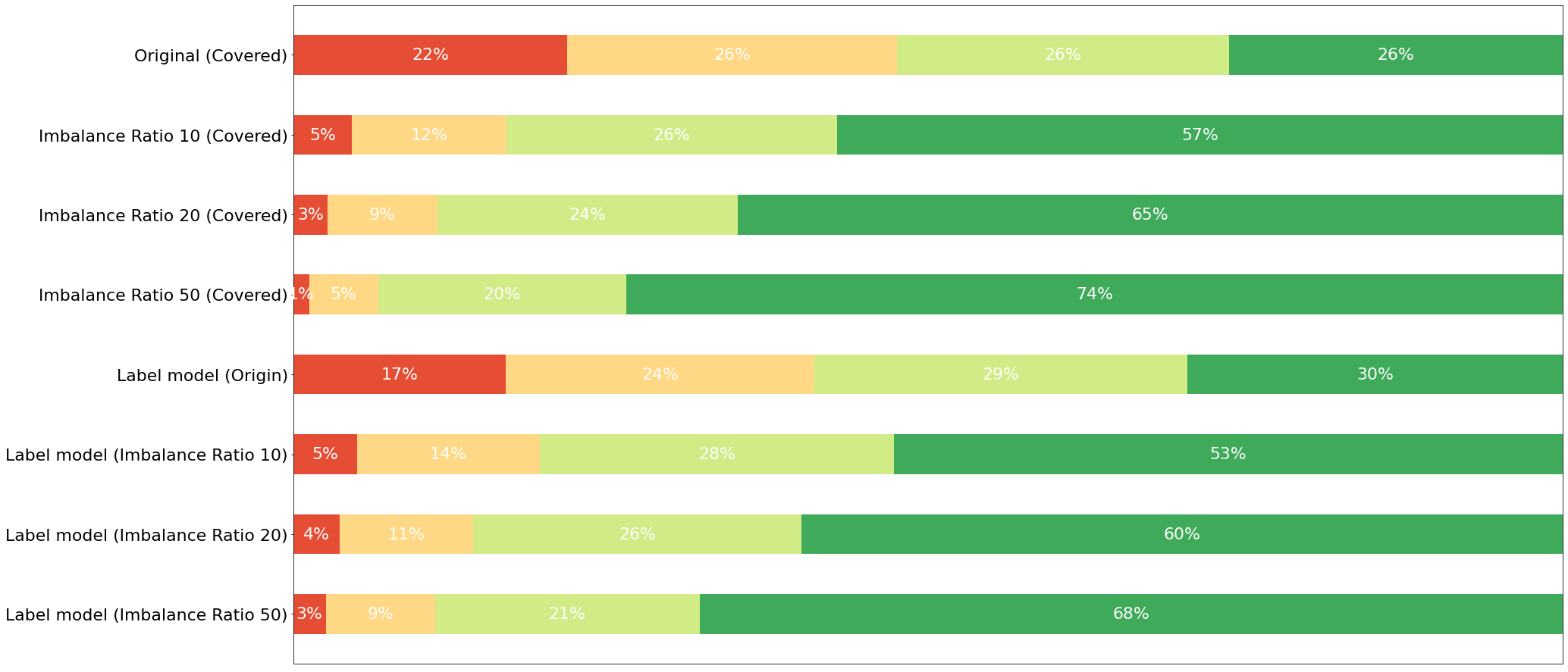
(a) AGNews

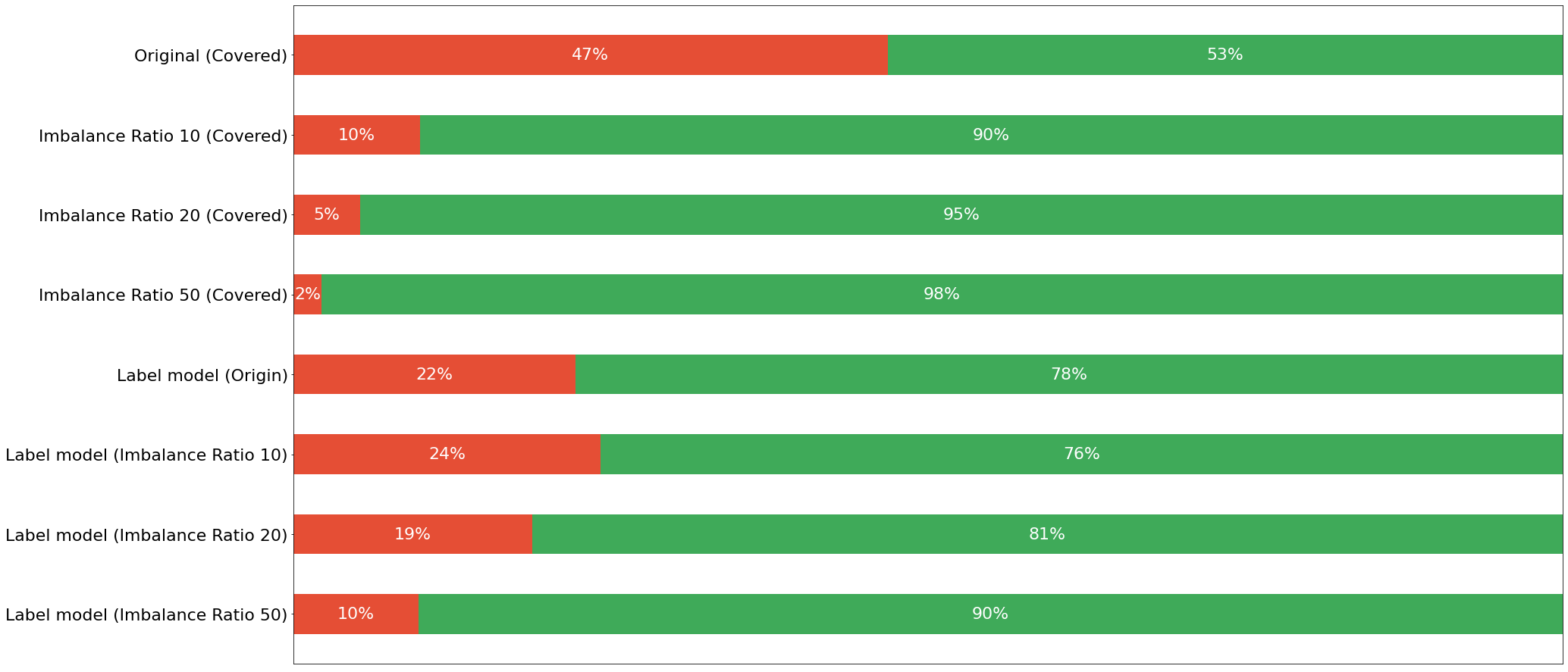
(b) Yelp

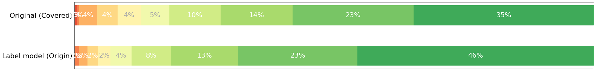
(c) Chemprot

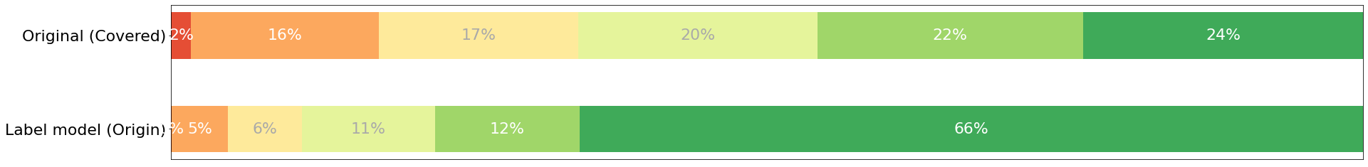
(d) TREC

Figure 6: Label statistic of each dataset.

For these two datasets, we design eight different imbalance ratios to evaluate all methods. The details are shown in Table 4 and the label distribution for each dataset are shown in Fig 6.

Dataset ($\downarrow$) Imbalance Ratio $\rho$ ($\downarrow$) Training Noise #Train #Train (Covered) #Valid AGNews 1 18.4% 96.0k 66.3k 12.0k 10 12.8% 42.7k 30.5k 5.4k 20 12.9% 37.3k 26.9k 4.7k 50 12.5% 32.8k 23.7k 4.1k Yelp 1 29.8% 30.4k 25.2k 3.8k 10 22.3% 16.8k 13.2k 2.0k 20 18.1% 16.0k 12.5k 1.9k 50 10.2% 15.6k 12.1k 1.9k

Table 4: Weakly Annotated Imbalance Dataset Statistics.

Appendix B Details on Implementation and Experiment Setups

B.1 Computing Infrastructure

System: Windows Subsystem Linux 2; Python 3.8; PyTorch 1.9.
CPU: Intel(R) Core(TM) i9-12900K CPU.
GPU: NVIDIA RTX 3090.

		Agnews (Imbalance Ratio ($\downarrow$))				Yelp (Imbalance Ratio ($\downarrow$))
Methods	Hyper-parameter	1	10	20	50	1	10	20	50
	Batch Size	128
	$\gamma$	3	10	1	1	1	1	1	1
	$\xi$	-0.2	-0.3	0	-0.2	0	-0.1	-0.1	-0.3
CE+LA	Dropout Ratio	0.2	0.2	0.0	0.2	0.2	0.0	0.0	0.0
	Learning Rate	0.001	0.001	0.003	0.001	0.001	0.0001	0.0001	0.0006
CE+EN	Dropout Ratio	0.2	0.0	0.0	0.0	0.2	0.0	0.0	0.0
	Learning Rate	0.001	0.001	0.001	0.001	0.001	0.001	0.001	0.001
	$\beta_{EN}$	0.9999	0.999	0.9	0.99	0.9999	0.99	0.999	0.9999
	$\gamma_{EN}$	2.0	0.5	1.0	2.0	1.0	0.5	1.0	0.5
CE+EN+LA	Dropout Ratio	0.0	0.2	0.2	0.2	0.2	0.0	0.0	0.0
	Learning Rate	0.0001	0.001	0.001	0.001	0.001	0.01	0.001	0.001
	$\beta_{EN}$	0.9999	0.99	0.999	0.99	0.999	0.9	0.999	0.99
	$\gamma_{EN}$	2.0	0.5	0.5	0.5	2.0	1.0	0.5	0.5
Dice	Dropout Ratio	0.0	0.2	0.0	0.2	0.0	0.0	0.2	0.0
	Learning Rate	0.001	0.001	0.001	0.001	0.01	0.01	0.001	0.001
	$\alpha$	0.2	0.2	0.2	0.2	0.1	0.1	0.1	0.1
	$\gamma_{Dice}$	0.005	1.0	0.268	0.005	1.0	0.268	0.001	0.001
	Denominator Square	False	True	True	False	True	True	False	False
LDAM	Dropout Ratio	0.2	0.0	0.2	0.0	0.2	0.0	0.0	0.0
	Learning Rate	0.001	0.001	0.001	1e-5	0.001	0.001	1e-5	1e-5
	max margin	0.7	0.8	0.9	0.2	0.8	0.6	0.6	0.3
	$s$	4.0	1.0	1.0	16.0	4.0	1.0	1.0	10.0
COSINE	Learning Rate	1e-5	1e-5	3e-5	1e-5	3e-5	1e-5	3e-5	3e-5
	$T_{3}$	100	50	50	200	200	100	50	200
	$\lambda$	0.1	0.1	0.1	0.1	0.1	0.01	0.05	0.1
	$\gamma_{C}$	0.3	0.9	0.9	0.7	0.3	0.9	0.9	0.3
Denoise	Learning Rate	1e-5	3e-6	1e-6	3e-6	3e-5	3e-5	1e-5	3e-6
	Hidden Size	512	512	256	512	128	64	256	256
	$\alpha$	0.6
	$c_{1}$	0.1	0.1	0.3	0.3	0.7	0.3	0.5	0.1
	$c_{2}$	0.7	0.7	0.3	0.3	0.1	0.5	0.1	0.5

Table 5: Hyperparameter configurations for all baselines.

B.2 Number of Parameters

ARS2 and all baselines use 2-layer MLP and Roberta-base Liu et al. (2019) with a task-specific classification head on the top as the backbone. The 2-layer MLP has 128 neural unit in each layer, the total parameters are $128\times 128\times number\ of\ classes$. The Roberta-base model contains 125M trainable parameters, and we fine-tune the last 4 layers with token size 512. We do not introduce any other parameters in our experiments.

B.3 Experiment Setups

All of our methods and baselines are run with 5 different random seeds and the result is based on the average performance on them. This indeed creates $8$ (the number of datasets with four imbalance ratios) $\times$ $5$ (the number of random seeds) $\times$ $12$ (the number of methods) $\times$ $2$ (the number of end models, MLP and RoBERTa) = $960$ experiments for fine-tuning, which is almost the limit of our computational resources, not to mention grid search for hyperparameter for each method. We have shown both the mean and the standard deviation of the performance criteria in our experiment sections.

B.4 Implementations Baselines

For these three methods listed below, since they are mainly used in CV tasks; thus the code is hard to directly used for our experiments. We re-implement these methods based on their implementations in WRENCH codebase.

EN

: https://github.com/richardaecn/class-balanced-loss.

LA

: https://github.com/google-research/google-research/tree/master/logit_adjustment.

LDAM

: https://github.com/kaidic/LDAM-DRW.

For these two weak supervision baselines listed below, we use the implementation provided by WRENCH.

COSINE, Denoise

: https://github.com/JieyuZ2/wrench.

Our implementation of ARS2 will be published upon acceptance.

B.5 Hyperparameters for General Experiments

We use AdamW Loshchilov and Hutter (2019) as the optimizer, and the learning rate of 2-layer MLP is chosen from $1\times 10^{-5}$ to $1\times 10^{-1}$, and $1\times 10^{-5},3\times 10^{-5},1\times 10^{-6},3\times 10^{-6}$ for RoBERTa. Dropout rate of 2-layer MLP is chosen from $0,0.2$. We set weight decay rate as $0$ and batch size as $128$ for 2-layer MLP, and weight decay rate as $1\times 10^{-4}$ and batch size as $16$ for RoBERTa. We warm-up and continual training until early stop, and evaluate 2-layer MLP in every 100 steps and RoBERTa every 5 steps. Finally, we use the model with the best performance on the development set for testing. The general hyperparameters we use are shown in Table 5.

B.6 Hyperparameters for ARS2

The hyperparameter of ARS2 includes $\gamma,\xi$ thus it does not require heavy hyperparameter tuning. In our experiments, we search $\gamma$ from $1$ to $10$, and $\xi$ from $-0.5$ to $0.5$.

B.7 Hyperparameters for Loss Modification Baselines

For loss modification methods, we mainly tune their key hyperparameters. For EN Cui et al. (2019), we tune the number for effective number $\beta$ from $[0.9,0.99,0.999,0.9999]$, $\gamma$ from $[0.5,1,2]$ and report the best performance. For LA Menon et al. (2020), they use $\tau$ to scale the prior ratio. But in our experiment, we directly set $\tau$ as $1$ to achieve LA’s performance as efficiently as possible. For Dice Li et al. (2019), it use $\alpha$ to scale the $(1-p)$ factor avoiding it become too large, we search $\alpha$ from $0.1$ to $1$. $\gamma_{Dice}$ is designed to help numerator and denominator become smooth, we search $\gamma_{Dice}$ from $1\times 10^{-4}$ to 1. Denominator square is designed to control the size of denominator, we search this hyperparameter in [True, False]. For LDAM Cao et al. (2019a), we search max margin from $0.1$ to $0.9$ and $s$ from $1$ to $30$.

B.8 Hyperparameters for Weak Supervision Baselines

For COSINE Yu et al. (2020), we search learning rate from $[1\times 10^{-5},3\times 10^{-5},1\times 10^{-6},3\times 10^{-6}]$, teacher model update frequency from $[50,100,200]$, regularize power scale from $[0.01,0.05,0.1]$ and margin threshold $\gamma_{C}$ from $[0.1,0.3,0.5,0.7,0.9]$. For Denoise Ren et al. (2020), we search learning rate from $[1\times 10^{-5},3\times 10^{-5},1\times 10^{-6},3\times 10^{-6}]$, denoiser hidden size from $[64,128,256,512]$ and $c_{1},c_{2}$ from $[0.1,0.3,0.5,0.7,0.9]$.

References

- Arpit et al. (2017) Devansh Arpit, Stanisław Jastrzębski, Nicolas Ballas, David Krueger, Emmanuel Bengio, Maxinder S Kanwal, Tegan Maharaj, Asja Fischer, Aaron Courville, Yoshua Bengio, et al. 2017. A closer look at memorization in deep networks. In International conference on machine learning, pages 233–242. PMLR.
- Awasthi et al. (2020) Abhijeet Awasthi, Sabyasachi Ghosh, Rasna Goyal, and Sunita Sarawagi. 2020. Learning from rules generalizing labeled exemplars. arXiv preprint arXiv:2004.06025.
- Blum and Mitchell (1998) A. Blum and Tom. Mitchell. 1998. Combining labeled and unlabeled data with co-training. In COLT.
- Cao et al. (2019a) Kaidi Cao, Colin Wei, Adrien Gaidon, Nikos Arechiga, and Tengyu Ma. 2019a. Learning imbalanced datasets with label-distribution-aware margin loss. arXiv preprint arXiv:1906.07413.
- Cao et al. (2019b) Kaidi Cao, Colin Wei, Adrien Gaidon, Nikos Arechiga, and Tengyu Ma. 2019b. Learning imbalanced datasets with label-distribution-aware margin loss. arXiv preprint arXiv:1906.07413.
- Chawla et al. (2002) Nitesh V Chawla, Kevin W Bowyer, Lawrence O Hall, and W Philip Kegelmeyer. 2002. Smote: synthetic minority over-sampling technique. Journal of artificial intelligence research, 16:321–357.
- Chen et al. (2020) Xuxi Chen, Wuyang Chen, Tianlong Chen, Ye Yuan, Chen Gong, Kewei Chen, and Zhangyang Wang. 2020. Self-pu: Self boosted and calibrated positive-unlabeled training. In International Conference on Machine Learning, pages 1510–1519. PMLR.
- Collell et al. (2016) Guillem Collell, Drazen Prelec, and Kaustubh Patil. 2016. Reviving threshold-moving: a simple plug-in bagging ensemble for binary and multiclass imbalanced data. arXiv preprint arXiv:1606.08698.
- Cui et al. (2019) Yin Cui, Menglin Jia, Tsung-Yi Lin, Yang Song, and Serge Belongie. 2019. Class-balanced loss based on effective number of samples. In Proceedings of the IEEE/CVF Conference on Computer Vision and Pattern Recognition (CVPR).
- Dawid and Skene (1979) Alexander Philip Dawid and Allan M Skene. 1979. Maximum likelihood estimation of observer error-rates using the em algorithm. Journal of the Royal Statistical Society: Series C (Applied Statistics), 28(1):20–28.
- Dodge et al. (2020) Jesse Dodge, Gabriel Ilharco, Roy Schwartz, Ali Farhadi, Hannaneh Hajishirzi, and Noah A. Smith. 2020. Fine-tuning pretrained language models: Weight initializations, data orders, and early stopping. CoRR, abs/2002.06305.
- Fan et al. (2017) Yanbo Fan, Siwei Lyu, Yiming Ying, and Bao-Gang Hu. 2017. Learning with average top-k loss. arXiv preprint arXiv:1705.08826.
- Fawcett and Provost (1996) Tom Fawcett and Foster J Provost. 1996. Combining data mining and machine learning for effective user profiling. In KDD, pages 8–13.
- Fu et al. (2020) Daniel Fu, Mayee Chen, Frederic Sala, Sarah Hooper, Kayvon Fatahalian, and Christopher Ré. 2020. Fast and three-rious: Speeding up weak supervision with triplet methods. In International Conference on Machine Learning, pages 3280–3291. PMLR.
- Gao et al. (2011) Huiji Gao, Geoffrey Barbier, and Rebecca Goolsby. 2011. Harnessing the crowdsourcing power of social media for disaster relief. IEEE Intelligent Systems, 26:10–14.
- Goodfellow et al. (2016) Ian Goodfellow, Yoshua Bengio, and Aaron Courville. 2016. Deep learning. MIT press.
- Gupta and Manning (2014) S. Gupta and Christopher D. Manning. 2014. Improved pattern learning for bootstrapped entity extraction. In CoNLL.
- Han et al. (2018) Bo Han, Quanming Yao, Xingrui Yu, Gang Niu, Miao Xu, Weihua Hu, Ivor Tsang, and Masashi Sugiyama. 2018. Co-teaching: Robust training of deep neural networks with extremely noisy labels. arXiv preprint arXiv:1804.06872.
- Hoffmann et al. (2011) R. Hoffmann, Congle Zhang, Xiao Ling, Luke Zettlemoyer, and Daniel S. Weld. 2011. Knowledge-based weak supervision for information extraction of overlapping relations. In ACL.
- Iranmehr et al. (2019) Arya Iranmehr, Hamed Masnadi-Shirazi, and Nuno Vasconcelos. 2019. Cost-sensitive support vector machines. Neurocomputing, 343:50–64.
- Jiang et al. (2018) Lu Jiang, Zhengyuan Zhou, Thomas Leung, Li-Jia Li, and Li Fei-Fei. 2018. Mentornet: Learning data-driven curriculum for very deep neural networks on corrupted labels. In International Conference on Machine Learning, pages 2304–2313. PMLR.
- Kang et al. (2019) Bingyi Kang, Saining Xie, Marcus Rohrbach, Zhicheng Yan, Albert Gordo, Jiashi Feng, and Yannis Kalantidis. 2019. Decoupling representation and classifier for long-tailed recognition. arXiv preprint arXiv:1910.09217.
- Kim and Kim (2020) Byungju Kim and Junmo Kim. 2020. Adjusting decision boundary for class imbalanced learning. IEEE Access, 8:81674–81685.
- King and Zeng (2001) Gary King and Langche Zeng. 2001. Logistic regression in rare events data. Political analysis, 9(2):137–163.
- Krallinger et al. (2017) Martin Krallinger, Obdulia Rabal, Saber A Akhondi, Martın Pérez Pérez, Jesús Santamaría, Gael Pérez Rodríguez, Georgios Tsatsaronis, Ander Intxaurrondo, José Antonio López, Umesh Nandal, et al. 2017. Overview of the biocreative vi chemical-protein interaction track. In Proceedings of the sixth BioCreative challenge evaluation workshop, volume 1, pages 141–146.
- Krishna et al. (2016) R. Krishna, Yuke Zhu, O. Groth, Justin Johnson, K. Hata, J. Kravitz, Stephanie Chen, Yannis Kalantidis, Li-Jia Li, D. Shamma, Michael S. Bernstein, and Li Fei-Fei. 2016. Visual genome: Connecting language and vision using crowdsourced dense image annotations. IJCV, 123:32–73.
- Kubat et al. (1997) Miroslav Kubat, Stan Matwin, et al. 1997. Addressing the curse of imbalanced training sets: one-sided selection. In Icml, volume 97, pages 179–186. Citeseer.
- Lan et al. (2020) Ouyu Lan, Xiao Huang, Bill Yuchen Lin, He Jiang, Liyuan Liu, and Xiang Ren. 2020. Learning to contextually aggregate multi-source supervision for sequence labeling. In ACL, pages 2134–2146.
- Li et al. (2019) Xiaoya Li, Xiaofei Sun, Yuxian Meng, Junjun Liang, Fei Wu, and Jiwei Li. 2019. Dice loss for data-imbalanced nlp tasks. arXiv preprint arXiv:1911.02855.
- Li and Roth (2002) Xin Li and Dan Roth. 2002. Learning question classifiers. In COLING 2002: The 19th International Conference on Computational Linguistics.
- Li et al. (2021) Yinghao Li, Pranav Shetty, Lucas Liu, Chao Zhang, and Le Song. 2021. Bertifying the hidden markov model for multi-source weakly supervised named entity recognition. In ACL, pages 6178–6190.
- Lison et al. (2020) Pierre Lison, Jeremy Barnes, Aliaksandr Hubin, and Samia Touileb. 2020. Named entity recognition without labelled data: A weak supervision approach. In ACL, pages 1518–1533.
- Liu et al. (2019) Yinhan Liu, Myle Ott, Naman Goyal, Jingfei Du, Mandar Joshi, Danqi Chen, Omer Levy, Mike Lewis, Luke Zettlemoyer, and Veselin Stoyanov. 2019. Roberta: A robustly optimized bert pretraining approach. arXiv preprint arXiv:1907.11692.
- Loshchilov and Hutter (2019) Ilya Loshchilov and Frank Hutter. 2019. Decoupled weight decay regularization. In International Conference on Learning Representations.
- Maloof (2003) Marcus A Maloof. 2003. Learning when data sets are imbalanced and when costs are unequal and unknown. In ICML-2003 workshop on learning from imbalanced data sets II, volume 2, pages 2–1.
- Mann and McCallum (2010) Gideon S. Mann and A. McCallum. 2010. Generalized expectation criteria for semi-supervised learning with weakly labeled data. J. Mach. Learn. Res., 11:955–984.
- Masnadi-Shirazi and Vasconcelos (2010) Hamed Masnadi-Shirazi and Nuno Vasconcelos. 2010. Risk minimization, probability elicitation, and cost-sensitive svms. In ICML.
- Menon et al. (2013) Aditya Menon, Harikrishna Narasimhan, Shivani Agarwal, and Sanjay Chawla. 2013. On the statistical consistency of algorithms for binary classification under class imbalance. In International Conference on Machine Learning, pages 603–611. PMLR.
- Menon et al. (2020) Aditya Krishna Menon, Sadeep Jayasumana, Ankit Singh Rawat, Himanshu Jain, Andreas Veit, and Sanjiv Kumar. 2020. Long-tail learning via logit adjustment. CoRR, abs/2007.07314.
- Mintz et al. (2009) Mike Mintz, Steven Bills, Rion Snow, and Daniel Jurafsky. 2009. Distant supervision for relation extraction without labeled data. In ACL, pages 1003–1011.
- Morik et al. (1999) Katharina Morik, Peter Brockhausen, and Thorsten Joachims. 1999. Combining statistical learning with a knowledge-based approach: a case study in intensive care monitoring. Technical report, Technical Report.
- Nguyen et al. (2017) An Thanh Nguyen, Byron Wallace, Junyi Jessy Li, Ani Nenkova, and Matthew Lease. 2017. Aggregating and predicting sequence labels from crowd annotations. In ACL, pages 299–309.
- Paszke et al. (2019) Adam Paszke, Sam Gross, Francisco Massa, Adam Lerer, James Bradbury, Gregory Chanan, Trevor Killeen, Zeming Lin, Natalia Gimelshein, Luca Antiga, et al. 2019. Pytorch: An imperative style, high-performance deep learning library. Advances in neural information processing systems, 32:8026–8037.
- Pleiss et al. (2020) Geoff Pleiss, Tianyi Zhang, Ethan Elenberg, and Kilian Q Weinberger. 2020. Identifying mislabeled data using the area under the margin ranking. Advances in Neural Information Processing Systems, 33:17044–17056.
- Provost (2000) Foster Provost. 2000. Machine learning from imbalanced data sets 101. In Proceedings of the AAAI’2000 workshop on imbalanced data sets, volume 68, pages 1–3. AAAI Press.
- Ratner et al. (2019a) A. J. Ratner, B. Hancock, J. Dunnmon, F. Sala, S. Pandey, and C. Ré. 2019a. Training complex models with multi-task weak supervision. In AAAI, pages 4763–4771.
- Ratner et al. (2019b) Alexander Ratner, Braden Hancock, Jared Dunnmon, Frederic Sala, Shreyash Pandey, and Christopher Ré. 2019b. Training complex models with multi-task weak supervision. In Proceedings of the AAAI Conference on Artificial Intelligence, volume 33, pages 4763–4771.
- Ratner et al. (2016a) Alexander J Ratner, Christopher M De Sa, Sen Wu, Daniel Selsam, and Christopher Ré. 2016a. Data programming: Creating large training sets, quickly. Advances in neural information processing systems, 29.
- Ratner et al. (2016b) Alexander J Ratner, Christopher M De Sa, Sen Wu, Daniel Selsam, and Christopher Ré. 2016b. Data programming: Creating large training sets, quickly. In NeurIPS, volume 29, pages 3567–3575.
- Ren et al. (2020) Wendi Ren, Yinghao Li, Hanting Su, David Kartchner, Cassie Mitchell, and Chao Zhang. 2020. Denoising multi-source weak supervision for neural text classification. arXiv preprint arXiv:2010.04582.
- Rühling Cachay et al. (2021) Salva Rühling Cachay, Benedikt Boecking, and Artur Dubrawski. 2021. End-to-end weak supervision. Advances in Neural Information Processing Systems, 34.
- Safranchik et al. (2020) Esteban Safranchik, Shiying Luo, and Stephen Bach. 2020. Weakly supervised sequence tagging from noisy rules. In AAAI, volume 34, pages 5570–5578.
- Takamatsu et al. (2012) Shingo Takamatsu, Issei Sato, and H. Nakagawa. 2012. Reducing wrong labels in distant supervision for relation extraction. In ACL.
- Tan et al. (2020) Jingru Tan, Changbao Wang, Buyu Li, Quanquan Li, Wanli Ouyang, Changqing Yin, and Junjie Yan. 2020. Equalization loss for long-tailed object recognition. In Proceedings of the IEEE/CVF conference on computer vision and pattern recognition, pages 11662–11671.
- Wallace et al. (2011) Byron C Wallace, Kevin Small, Carla E Brodley, and Thomas A Trikalinos. 2011. Class imbalance, redux. In 2011 IEEE 11th international conference on data mining, pages 754–763. IEEE.
- Wei et al. (2021) Chen Wei, Kihyuk Sohn, Clayton Mellina, Alan Yuille, and Fan Yang. 2021. Crest: A class-rebalancing self-training framework for imbalanced semi-supervised learning. In Proceedings of the IEEE/CVF Conference on Computer Vision and Pattern Recognition, pages 10857–10866.
- Wu et al. (2018) Xiang Wu, Ran He, Zhenan Sun, and Tieniu Tan. 2018. A light cnn for deep face representation with noisy labels. IEEE Transactions on Information Forensics and Security, 13(11):2884–2896.
- Xie and Manski (1989) Yu Xie and Charles F Manski. 1989. The logit model and response-based samples. Sociological Methods & Research, 17(3):283–302.
- Yao et al. (2020) Quanming Yao, Hansi Yang, Bo Han, Gang Niu, and James Tin-Yau Kwok. 2020. Searching to exploit memorization effect in learning with noisy labels. In International Conference on Machine Learning, pages 10789–10798. PMLR.
- Ye et al. (2020) Han-Jia Ye, Hong-You Chen, De-Chuan Zhan, and Wei-Lun Chao. 2020. Identifying and compensating for feature deviation in imbalanced deep learning. arXiv preprint arXiv:2001.01385.
- Yu et al. (2019) Xingrui Yu, Bo Han, Jiangchao Yao, Gang Niu, Ivor W Tsang, and Masashi Sugiyama. 2019. How does disagreement benefit co-teaching. arXiv preprint arXiv:1901.04215, 3.
- Yu et al. (2020) Yue Yu, Simiao Zuo, Haoming Jiang, Wendi Ren, Tuo Zhao, and Chao Zhang. 2020. Fine-tuning pre-trained language model with weak supervision: A contrastive-regularized self-training approach. arXiv preprint arXiv:2010.07835.
- Zaidan and Eisner (2008) Omar Zaidan and Jason Eisner. 2008. Modeling annotators: A generative approach to learning from annotator rationales. In EMNLP.
- Zhang et al. (2022a) Jieyu Zhang, Cheng-Yu Hsieh, Yue Yu, Chao Zhang, and Alexander Ratner. 2022a. A survey on programmatic weak supervision. arXiv preprint arXiv:2202.05433.
- Zhang et al. (2022b) Jieyu Zhang, Bohan Wang, Xiangchen Song, Yujing Wang, Yaming Yang, Jing Bai, and Alexander Ratner. 2022b. Creating training sets via weak indirect supervision. In ICLR.
- Zhang et al. (2021) Jieyu Zhang, Yue Yu, Yinghao Li, Yujing Wang, Yaming Yang, Mao Yang, and Alexander Ratner. 2021. Wrench: A comprehensive benchmark for weak supervision. In Thirty-fifth Conference on Neural Information Processing Systems Datasets and Benchmarks Track (Round 2).
- Zhang et al. (2015) Xiang Zhang, Junbo Zhao, and Yann LeCun. 2015. Character-level convolutional networks for text classification. Advances in neural information processing systems, 28:649–657.
- Zhang et al. (2017) Xiao Zhang, Zhiyuan Fang, Yandong Wen, Zhifeng Li, and Yu Qiao. 2017. Range loss for deep face recognition with long-tailed training data. In Proceedings of the IEEE International Conference on Computer Vision, pages 5409–5418.
- Zheng et al. (2020) Songzhu Zheng, Pengxiang Wu, Aman Goswami, Mayank Goswami, Dimitris Metaxas, and Chao Chen. 2020. Error-bounded correction of noisy labels. In International Conference on Machine Learning, pages 11447–11457. PMLR.