High-energy neutrinos from choked-jet supernovae: searches and implications

Abstract

The origin of the high-energy astrophysical neutrinos discovered by IceCube remains largely unknown. Multi-messenger studies have indicated that the majority of these neutrinos come from gamma-ray-dark sources. Choked-jet supernovae (cjSNe), which are supernovae powered by relativistic jets stalled in stellar materials, may lead to neutrino emission via photohadronic interactions while the coproduced gamma rays are absorbed. In this paper, we perform an unbinned-maximum-likelihood analysis to search for correlations between IceCube’s 10-year muon-track events and our SN Ib/c sample, collected from publicly available catalogs. In addition to the conventional power-law models, we also consider the impacts of more realistic neutrino emission models for the first time, and study the effects of the jet beaming factor in the analyses. Our results show no significant correlation. Even so, the conservative upper limits we set to the contribution of cjSNe to the diffuse astrophysical neutrino flux still allow SNe Ib/c to be the dominant source of astrophysical neutrinos observed by IceCube. We discuss implications to the cjSNe scenario from our results and the power of future neutrino and supernova observations.

I Introduction

The discovery of high-energy (HE) astrophysical neutrinos by the IceCube Neutrino Observatory Aartsen et al. (2013a, b) has opened a new era of neutrino physics, astrophysics, and multimessenger astronomy. These neutrinos are nearly isotropic on the sky and have energies between 10 TeV to above PeV, suggesting their sources to be the extragalactic populations of extreme cosmic accelerators. Searching for HE neutrino sources is also crucial to identify sources of their parent HE cosmic rays and it offers unique opportunities to understand the acceleration mechanisms of the sources.

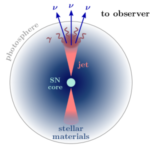
Figure 1: Schematic view of a core-collapse supernova with its jet choked inside the dense envelope of a progenitor star or external circumstellar materials. While neutrinos and gamma rays are both produced by the cosmic rays inside the jet, only neutrinos can freely escape from the optically thick medium.

Various astrophysical objects have been studied as the sources of the HE neutrinos, such as gamma-ray bursts (GRBs) Paczynski and Xu (1994); Waxman and Bahcall (1997); Dermer and Atoyan (2003); Kimura (2022), active galactic nuclei (AGN) Berezinsky (1977); Eichler (1979); Stecker et al. (1991); Murase (2017), supernovae (SNe) Murase et al. (2011); Murase (2018), tidal disruption events (TDEs) Murase (2008); Wang and Liu (2016); Dai and Fang (2017); Senno et al. (2017); Lunardini and Winter (2017), and so on. Motivated by multi-messenger observations of electromagnetic and gravitational-wave signals, significant efforts have been put into searching for the sources over the past decade. Compelling evidence for a few point sources has been reported: blazar TXS 0506+056 Aartsen et al. (2018a, b), Seyfert II galaxy NGC 1068 Aartsen et al. (2020a), and TDE candidates AT2019dsg, AT2019fdr, and AT2019aalc Stein et al. (2021); Reusch et al. (2022); van Velzen et al. (2021). However, stacking analyses show that none of the aforementioned types of sources contribute a major fraction of the all-sky neutrino flux (a possible exception might be the non-jetted AGN if the observed 2.6$\sigma$ significance is interpreted as a signal Abbasi et al. (2022)). Furthermore, the measurement of the extragalactic gamma-ray background by the Fermi Large Area Telescope (LAT) Ackermann et al. (2015) has set robust constraints on gamma-ray-bright sources as dominant HE neutrino emitters, as a comparable flux of gamma rays are expected to be coproduced with neutrinos following $pp$ and $p\gamma$ interactions of cosmic rays Murase et al. (2013). Thus, it is likely that there is a class of HE neutrino sources opaque to GeV – TeV gamma rays, in which only neutrinos can freely escape from the cosmic-ray accelerators Murase et al. (2016); Capanema et al. (2020, 2021); Fang et al. (2022); Fasano et al. (2021).

Choked-jet supernovae (cjSNe) are promising as such hidden neutrino sources Meszaros and Waxman (2001); Razzaque et al. (2004, 2005); Ando and Beacom (2005); Murase and Ioka (2013); He et al. (2018). Figure 1 shows an illustration: in this scenario, the jets are stalled or “choked” inside the progenitor envelopes or circumstellar materials as they are not powerful enough. Gamma rays produced from cosmic rays accelerated in the choked jet are attenuated through optically thick environments below the stellar photosphere, leaving HE neutrinos as primary signals. Previous theoretical studies have shown that cjSNe could even explain all the HE astrophysical neutrinos observed by IceCube Murase and Ioka (2013); Tamborra and Ando (2016); Senno et al. (2016); Guetta et al. (2020); Carpio and Murase (2020).

In addition, cjSN provides a unified scenario for Type Ib/c supernovae (SNe Ib/c), hypernovae, and the different types of GRBs, in which jet properties and shock-breakout conditions are crucial in making the difference Nakar (2015); Senno et al. (2016). The link to low-power (LP) GRBs such as low-luminosity (LL) GRBs and ultralong (UL) GRBs further strengthens the role of cjSNe as gamma-ray dark factories of HE neutrinos Murase and Ioka (2013); Senno et al. (2016); Carpio and Murase (2020). From the observational side, many LP GRBs are missed by current GRB surveys, so current stringent limits on HE neutrino emission from classical, high-luminosity GRBs do not apply. From the theoretical side, the intrinsically weak jets associated with LP GRBs are more ideal for neutrino production than classical GRBs, as powerful jets generally lead to inefficient cosmic-ray acceleration in radiation-mediated shocks Murase and Ioka (2013). Therefore, HE neutrinos also provide us with an essential tool to study the cjSN scenario and the observed GRB-SN connection Galama et al. (1998); Hjorth et al. (2003); Stanek et al. (2003); Modjaz et al. (2016).

In this paper, we search for HE neutrinos from cjSNe and study the theoretical implications. Previous studies Abbasi et al. (2011, 2012); Senno et al. (2018); Esmaili and Murase (2018); Necker et al. (2021) have performed searches using early datasets of IceCube and found no association of neutrinos with supernovae. Here we use 10 years of IceCube neutrino data Abbasi et al. (2021a); () (2021), in which high-quality events are recorded and have never been analyzed for cjSNe. We perform an unbinned-maximum-likelihood analysis to search for a statistical correlation between neutrinos and SNe Ib/c, as cjSNe can in principle be observed as SNe Ib/c, where progenitor stars are more massive and typically enclosed by denser extended materials. Our analyses do not find any excess of neutrinos from SNe Ib/c with respect to the background, from which we set upper limits on cjSN models and their contribution to the total astrophysical neutrino fluxes observed by IceCube. Figure 2 illustrates how muon-neutrino signals from all SNe Ib/c in our analyzed sample would look in IceCube, assuming the highest cjSN flux allowed by our analysis.

Figure 2: A schematic prediction of the muon-track events produced by our 10-year SNe Ib/c sample as a function of the reconstructed muon-energy $E_{\mu}$ in IceCube. Here, the signal events are from the cjSN model with a $E_{\nu}^{-2}$ neutrino spectrum with parameters $\{\mathcal{E}_{\rm CR},f_{\rm jet}\}$ (detailed in Sec. IV) defined by the upper limit from our analysis. In comparison, we also show the effective number of background events associated with the supernovae [within the effective size of time (20 days) and spatial window (9 ${\rm deg}^{2}$); in our analyses, we use more events than shown here (Sec. III.2)]. The sensitivity of our analysis is mainly driven by the neutrino data with energy above few tens of TeV, where the background becomes negligible compared to the signal.

For the first time, we take into account physical models of neutrino emission in LP GRBs, instead of simply assuming HE neutrinos to follow power-law spectra. This is important, as the astrophysical neutrino flux may originate from multiple source populations with various neutrino spectra. Moreover, as the current LP GRB sample is highly incomplete and model uncertainties of LP GRBs are largely unconstrained, our survey in model parameters using SNe Ib/c catalogs is meaningful. Finally, our conservative limits show that, for most cjSN models we consider, SNe Ib/c can still account for 100% of the IceCube diffuse neutrino flux. Moreover, we find that, even with a very conservative approach, 10 years of IceCube data are almost probing all cjSN models, thus implying cjSNe will be robustly tested as HE neutrino sources in the near future.

This paper is organized as follows. In Sec. II, we describe the neutrino dataset and the supernova sample we use and introduce the cjSN models we consider. In Sec. III, we discuss our likelihood formalism and how we obtain the correlation significance from background simulation. In Sec. IV, we detail the procedures of setting upper limits, including how we simulate neutrino signals from cjSNe and how we look for an excess of signals among background fluctuations. In Sec. V, we show our results from single-source and stacking analyses, and present constraints on cjSN models and their contributions to the HE astrophysical neutrino fluxes observed by IceCube. We further discuss the implications of cjSNe as the origin of HE neutrinos. We then comment on the difference between our results and those in Ref. Necker et al. (2021). In Sec. VI, we conclude our findings with a future roadmap.

II Data and Models

II.1 10 years of IceCube neutrino data

The IceCube Neutrino Observatory detects neutrinos through the Cherenkov photons emitted by relativistic charged particles produced from neutrino interactions in (starting events) and outside (throughgoing events) the detector Achterberg et al. (2006); ICw . The Cherenkov photons trigger the nearby digital optical modules and can form two kinds of basic event topologies: elongated tracks formed by muons and showers which looks like a round and big blob formed by electrons (electromagnetic shower) or hadrons (hadronic shower). The track events, which are dominated by throughgoing tracks, have a much better angular resolution (as good as $<1^{\circ}$) though worse energy resolution ($\sim 200\%$ at $\sim 100$ TeV) than the shower events ($\sim$ $10^{\circ}$ – $15^{\circ}$ and $\sim 15\%$ above 100 TeV) ICr . Thus, track events are suited to search for point sources.

The data released by the IceCube Collaboration span from April 2008 to July 2018 Abbasi et al. (2021a); () (2021). The same data have been used in the 10-year time-integrated neutrino point-source search by IceCube collaboration Aartsen et al. (2020b) and searching for high-energy neutrino emission from radio bright AGN Zhou et al. (2021). In total, there are 1,134,450 muon-track events. The information for each track is provided, including arrival time, angular direction, angular error, and reconstructed energy. The arrival time is given in precision of $1\times 10^{-8}$ days ($8.6\times 10^{-4}$ s). These ten years of data are grouped into five samples corresponding to different construction phases of IceCube and instrumental response functions, including 1) IC40, 2) IC59, 3) IC79, 4) IC86-I, and 5) IC86-II to IC86-VII. The numbers in the names represent the numbers of strings in the detector on which digital optical modules are deployed. Distributions of these events in the sky can be found in Figs. 1 and 2 in Ref. Zhou et al. (2021). We use the events with declination (Dec) between $-10^{\circ}$ and $90^{\circ}$ for the following reasons. First, the events from $\rm Dec<-10^{\circ}$ (southern sky with respect to IceCube) have much higher backgrounds from atmospheric muons Abbasi et al. (2021a). Second, we find that the given smearing matrices from simulations have too low statistics to obtain good enough energy PDFs for our analysis (Sec. III.2).

We also process the $19\times 2$ double-counted tracks in the dataset found in Ref. Zhou and Beacom (2022) (listed in its table III). These events arise from an internal reconstruction error that identifies some single muons crossing the dust layer as two separate muons arriving at the same time and closely in direction Zhou and Beacom (2022). This would affect neutrino-source searches, especially transients, as finding two associated events versus one would be quite different. Thus, we combine the 19 misreconstructed pairs into 19 single events by averaging the directions and summing up the reconstructed energies.

II.2 Supernova sample

The supernova sample we use for our analysis is from combining SNe Ib/c from the Open Supernova Catalog Guillochon et al. (2017), the Weizmann Interactive Supernova Data Repository (WISeREP) Yaron and Gal-Yam (2012), and the All-Sky Automated Survey for Supernovae (ASAS-SN) Holoien et al. (2017a, b, c, 2019). These catalogs have collected more than 36,000, 20,000, and 1,300 supernovae, respectively, from a variety of astronomical surveys and existing archives. We further compare our combined supernova sample with the publicly available catalog of bright supernovae BSN ; Gal-Yam et al. (2013) and incorporate those that are missed in the above.

Sometimes a supernova is independently discovered by different groups and thus has multiple aliases. This leads to a small fraction of potentially duplicate sources in our sample. To avoid double counting, we first search for the supernovae with an angular distance smaller than $0.1^{\circ}$. We then merge these supernovae if they are classified as the same type and the difference in their maximal brightness time and redshift are less than 30 days and $10\%$, respectively. The examples of supernova pairs satisfying our criteria are {SN 2010O, SN 2010P} and {SN 2016coi, ASASSN-16fp}. As these potentially duplicate sources have very similar observational properties, we remove one of them from our sample.

Finally, we keep the supernovae in our sample only if they were observed at ${\rm Dec}\geq-10^{\circ}$ and within the uptime of IceCube between April 2008 and July 2018 to match our selected data (Sec. II.1). In total, our final sample consists of 386 SNe Ib/c, including 30, 36, 36, 36, and 248 for IC40, IC59, IC79, IC86-I, and IC86-II – VII, respectively. We provide the details of our supernova sample at this URL .

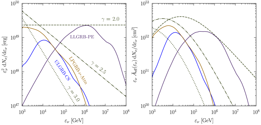
Figure 3: A comparison of single-burst neutrino spectra from the cjSN models we consider. Here, the LLGRB-PE model involves prompt neutrino emission from low-luminosity GRBs Murase et al. (2006); the ULGRB-CS model involves neutrinos from cosmic rays accelerated at the collimation shock of ultra-long-duration GRBs Murase and Ioka (2013); and the LPGRB-$\nu$-Attn model involves neutrinos attenuated in the progenitor star of low-power GRBs Carpio and Murase (2020). All spectra are normalized to have the same isotropic equivalent cosmic ray energy, $\mathcal{E}_{\rm CR}=10^{51}$ erg. Both panels use the same line style for each model while in the right panel each spectrum is weighted by the IceCube effective area (averaged over ${\rm Dec}\geq-10^{\circ}$). The realistic modeling of cjSNe takes into account a variety of cooling mechanisms, leading to the suppression in the neutrino spectra and different energy distributions of neutrino events detected by IceCube.

II.3 cjSN models for neutrino emission

We assume choked jets to be nearly calorimetric sources (except the suppression factor) so that neutrinos are produced by all available energy $\mathcal{E}_{\rm CR}$ in cosmic rays. The all-flavor neutrino spectrum from a single burst of supernova is thus given by Waxman and Bahcall (1999); Murase and Bartos (2019)

$$\left.\frac{{\rm d}N_{\nu}(\varepsilon_{\nu};\mathcal{E}_{\rm CR})}{{\rm d}\varepsilon_{\nu}}\right|_{\varepsilon_{\nu}=0.05\varepsilon_{p}}\approx\frac{3}{8}f_{\rm sup}\,{\rm min}[1,f_{p\gamma}]\frac{\mathcal{E}_{\rm CR}}{{\mathcal{R}}_{p}(\varepsilon_{p})}\varepsilon_{\nu}^{-2}\,,$$ (1)

where the factor $3/8$ is the fraction of energy taken away by neutrinos from charged pions produced in the $p\gamma$ interactions; the energy-dependent suppression factor $f_{\rm sup}(\varepsilon_{p})$ accounts for the meson and muon cooling processes that depend on the detailed modeling of choked jets; and the meson production efficiency ${\rm min}[1,\,f_{p\gamma}]$ is set to $1$ for the choked jets as long as the minimal cosmic-ray energy is larger than the pion production threshold. As the average fraction of energy transferred from a parent proton to each neutrino after an interaction is $1/20$, we have $\varepsilon_{\nu}\approx(1/20)\varepsilon_{p}$. ${\mathcal{R}}_{p}$ denotes the bolometric correction factor for the cosmic-ray spectrum. The cosmic rays are expected to follow a power-law spectrum Waxman (1995) (i.e., ${\rm d}N_{p}/{\rm d}\varepsilon_{p}\propto\varepsilon_{p}^{-\gamma}$) as they are typically accelerated through the first-order Fermi process Fermi (1949) in the shock. In this case, we have ${\mathcal{R}}_{p}(\varepsilon_{p})=\ln{(\varepsilon_{p}^{\rm max}/\varepsilon_{p}^{\rm min})}$ for $\gamma=2$ and ${\mathcal{R}}_{p}(\varepsilon_{p})={(\gamma-2)^{-1}[1-(\varepsilon_{p}^{\rm max}/\varepsilon_{p}^{\rm min})^{2-\gamma}](\varepsilon_{p}/\varepsilon_{p}^{\rm min})^{\gamma-2}}$ for $\gamma\neq 2$. When producing our results in Sections V.2 and V.3, we take $(\varepsilon_{p}^{\rm min},\varepsilon_{p}^{\rm max})=(2\times 10^{3},2\times 10^{10})\,{\rm GeV}$ as this leads to efficient neutrino production within $(\varepsilon_{\nu}^{\rm min},\varepsilon_{\nu}^{\rm max})\approx(10^{2},10^{9})\,{\rm GeV}$, the energy range that could be detected by IceCube.

We also consider two well-motivated cjSN models Murase et al. (2006); Murase and Ioka (2013). Both models assume power-law parent cosmic-ray spectra with $\gamma=2.0$ but the neutrino spectra are different due to various processes of meson and muon cooling in different shocked regions of the jet. In reality, $f_{p\gamma}$ in Eq. 1 is below the unity at low energies and that $f_{\rm sup}<1$ is possible depending on cjSN parameters.

Our first class of models assumes the neutrino spectrum to follow a power law with the same spectral index ($\gamma$) as the parent proton spectrum. This neglects all complicated mechanisms that could lead to a nontrivial neutrino spectrum. We consider $\gamma=2.0$, $\gamma=2.5$, and $\gamma=3.0$ as three benchmark models, which match the best fits to the 10 years of muon-track events Stettner (2020), a combination of track and shower events Aartsen et al. (2015a, 2020c), and the 7.5 years of the high-energy starting events (HESE) Abbasi et al. (2021b), respectively.

Our second class of models takes into account more realistic modeling that links cjSNe with LL GRBs and UL GRBs. We consider three physical models from different detailed considerations of jet propagation inside the progenitor star and energy losses of particles: 1) the LLGRB-PE model (prompt $\nu$ emission from LL GRBs) Murase et al. (2006); 2) the ULGRB-CS model (neutrinos from cosmic rays accelerated at the collimation shock of UL GRBs) Murase and Ioka (2013); and 3) the LPGRB-$\nu$-Attn model (attenuated neutrinos from LP GRBs) Carpio and Murase (2020). Note that the model spectrum used in this work takes into account the inverse-Compton cooling of pions and muons, which slightly affects the flux above $\sim 0.1-1$ PeV compared to the original reference.

Figure 3 left panel shows that for the same $\mathcal{E}_{\rm CR}$, the all-flavor neutrino spectra of a supernova burst from different models can differ by several orders of magnitude at certain energies. The y-axis is shown as $\varepsilon_{\nu}^{2}{\rm d}N_{\nu}/{\rm d}\varepsilon_{\nu}=2.3^{-1}\varepsilon_{\nu}{\rm d}N_{\nu}/{\rm d}\log\varepsilon_{\nu}$ so that the area under each curve is proportional to the total energy of neutrinos. Figure 3 right panel shows the spectra of detectable muon neutrinos in IceCube, calculated from the curves in the left panel and the average IceCube effective area $\bar{A}_{\rm eff}$ over ${\rm Dec}\geq-10^{\circ}$. For comparison, here we assume that neutrinos are evenly distributed among all flavors. The y-axis is shown as $\varepsilon_{\nu}\bar{A}_{\rm eff}{\rm d}N_{\nu}/{\rm d}\varepsilon_{\nu}=2.3^{-1}\bar{A}_{\rm eff}{\rm d}N_{\nu}/{\rm d}\log\varepsilon_{\nu}$ so that the area under each curve is proportional to the total number of detected neutrinos. For the same $\mathcal{E}_{\rm CR}$, power-law models (in which there are no cooling effects) or physical models with harder emission spectra between 10 TeV and 1 PeV (where IceCube has the best sensitivity) tend to produce more neutrino events in detectors.

III Analysis Formalism

III.1 Likelihood function and test statistic

To search for a possible correlation between IceCube events and supernovae, we use an unbinned maximum-likelihood method. A similar formalism was commonly used to search for transient neutrino sources by IceCube Abbasi et al. (2010, 2009); Aartsen et al. (2015b, 2016, 2017a, 2018c); Fahey et al. (2018); Aartsen et al. (2020d); Kheirandish et al. (2021) and other experiments Thrane et al. (2009). The likelihood function is defined as

$$\mathcal{L}(s,b)=\prod_{k}^{5}\prod_{j\in k}^{N^{k}_{\rm SN}}\left[p_{j}(s_{j},b_{j})\prod_{i\in j}^{N_{j}}\mathcal{L}^{k}_{ij}(s_{j},b_{j})\right]\,,$$ (2)

where $k$ labels the five data samples we use in our analysis, $N^{k}_{\rm SN}$ number of supernovae observed during the period of each data sample, and $N_{j}$ is the total number of muon-track events appearing in the temporal and spatial window of the $j$th supernova. Moreover, $s_{j}$ and $b_{j}$ are the signal and background event rates for the $j$th supernova, respectively. In our analysis, $s_{j}$ is the parameter to be determined by maximizing the likelihood function, and $b_{j}$ is computed by scaling the number of track events in the supernova’s spatial window and outside the temporal window by the ratio between the total time outside and inside its time window. Details of the windows are in Sec. III.2.

The $\mathcal{L}^{k}_{ij}(s_{j},b_{j})$ in Eq. (2) is the individual likelihood function of a track event $i$ from the $k$th data sample associated with the $j$th supernova,

$$\mathcal{L}^{k}_{ij}(s_{j},b_{j})=\frac{1}{{s_{j}+b_{j}}}\left(s_{j}S^{k}_{ij}+b_{j}B^{k}_{ij}\right)\,,$$ (3)

with $S_{ij}^{k}$ the signal probability density function (PDF) and $B_{ij}^{k}$ the background PDF, details in Sec. III.2.

The $p_{j}(s_{j},b_{j})$ in Eq. (2) is a weighting factor,

$$p_{j}(s_{j},b_{j})=\frac{(s_{j}+b_{j})^{N_{j}}{\rm e}^{-(s_{j}+b_{j})}}{N_{j}!}\,,$$ (4)

to take into account the Poisson fluctuations of $N_{j}$.

The test statistic (TS) is then defined as the ratio of the likelihood function to its value under the null hypothesis

$${\rm TS}\equiv 2\ln\left[\frac{\mathcal{L}(s,b)}{\mathcal{L}(0,b)}\right]\,.$$ (5)

From Eqs. 2, 3 and 4 we have

$${\rm TS} =\sum_{k}^{5}\sum_{j\in k}^{N^{k}_{\rm SN}}\,2\left[-s_{j}+\sum^{N_{j}}_{i\in j}\ln\left(\frac{s_{j}S^{k}_{ij}}{b_{j}B^{k}_{ij}}+1\right)\right]$$ (6)

$$\equiv\sum_{k}^{5}\sum_{j\in k}^{N^{k}_{\rm SN}}{\rm TS}^{k}_{j}\,,$$ (7)

where ${\rm TS}^{k}_{j}$ is the test statistic for a single source covered by the $k$th data sample. Comparing the TS values from the real with simulated data (details in Sec. III.3), we can get the significance (or p-value) of the correlation between the supernova sample and the real data.

III.2 Signal and background PDFs

Both signal and background PDFs for a track event are multiplications of temporal, spatial, and energy PDFs,

$$S^{k}_{ij} =S^{k}_{T,\,ij}\cdot S^{k}_{{\rm spt},\,ij}\cdot S^{k}_{E,\,ij}\,,$$ (8)

$$B^{k}_{i} =B^{k}_{T,\,ij}\cdot B^{k}_{{\rm spt},\,ij}\cdot B^{k}_{E,\,ij}\,.$$ (9)

These PDFs describe the expected temporal, spatial, and energy distributions of the events if they are from the sources or the background. For the background PDFs, we calculate them directly from data as they have enough statistics.

The signal temporal PDF is taken as a Gaussian distribution in $T_{\rm SN}-T_{\nu}$, the difference between the time of a supernova’s maximum brightness and the arrival time of an event,

$$S^{k}_{T,\,ij}(T_{i}|T_{{\rm SN}j})$$

$$=\frac{1}{\sqrt{2\pi\sigma_{T}^{2}}}\,{\rm exp}\left\{-\frac{[(T_{{\rm SN}j}-T_{i})-\lambda_{T}]^{2}}{2\sigma_{T}^{2}}\right\}\,,$$ (10)

where $\sigma_{T}=4$ days and $\lambda_{T}=13$ days given below.

In the standard scenarios of cjSNe, high-energy neutrinos and gamma rays are produced simultaneously via the interaction of relativistic jet inside the extended stellar envelope. As it is found that SNe Ib/c correlated with GRBs typically reach their maximal optical brightness after $\simeq 13$ days from the prompt gamma-ray emission Cano et al. (2017), we take $\lambda_{T}=13$ days in Eq. 10.

When searching for temporal correlation, the time window of each supernova is determined by the $99\%$ confidence interval of Eq. 10. This gives ${T_{{\rm SN}j}-T_{i}\in[\lambda_{T}-2.58\sigma_{T},\,\lambda_{T}+2.58\sigma_{T}]}$, the width of which is $\simeq 20$ days. The events outside the window are almost impossible to come from the supernova.

For the background temporal PDF, we use a uniform distribution inside the time window and zero outside,

$$B^{k}_{T,\,ij}(T_{i}|T_{{\rm SN}j})=\frac{1}{2\times 2.58\sigma_{T}}\,,$$ (11)

because the background event rate from high-energy atmospheric neutrinos and muon interactions are constant.

The signal spatial PDF is given by the Fisher-Bingham (Kent) distribution Fisher (1953); Bingham and Mardia (1978); Kent (1982),

$$S^{k}_{{\rm spt},\,ij}(\mu_{ij}|\sigma_{\nu i})=\frac{\sigma_{\nu i}^{-2}}{4\pi\,{\rm sinh}\,\left(\sigma_{\nu i}^{-2}\right)}\,{\rm exp}\left(\sigma_{\nu i}^{-2}\mu_{ij}\right),\,$$ (12)

where $\mu_{ij}=\cos(\Delta\psi_{ij})$, with $\Delta\psi_{ij}$ the angular distance between the track $i$ and supernova $j$, and $\sigma_{\nu i}$ is the reconstructed angular error of a track Abbasi et al. (2021a); () (2021). Equation 12 can be understood as a generalization of the 2D Gaussian distribution with the standard deviation $\sigma_{\nu i}$ on a sphere. For small $\Delta\psi_{ij}$, it reduces to a 2D Gaussian distribution.

Similar to the time window, we search for spatial correlation through the spatial window defined by the $99\%$ confidence interval of Eq. 12, which gives $\mu_{ij}\geq\mu_{99}(\sigma_{\nu i})$ where

$$\mu_{99}(\sigma_{\nu i})=1+\sigma_{\nu i}^{2}\ln\left\{1-0.99[1-{\rm exp}(-2\sigma_{\nu i}^{-2})]\right\}\,.$$ (13)

The background spatial PDF is a function of Dec, $\delta_{i}$, as distribution with respect to right ascension (RA) is nearly isotropic because IceCube locates at the South Pole. We use the same sliding-window method as in Ref. Zhou et al. (2021) to calculate the background spatial PDF. We normalize the background spatial PDF over a Dec from $-10^{\circ}$ to $90^{\circ}$, matching the data used in our analysis. The results can be found in Fig. 2 of Ref. Zhou et al. (2021).

The signal energy PDF of an event in sample $k$ can be calculated by

$$S^{k}_{E,\,ij}(E^{\rm prx}_{i}|\delta_{i})$$

$$\propto\int{\rm d}E_{\nu}\phi_{j}(E_{\nu})A^{k}_{\rm eff}(E_{\nu}|\delta_{i})P^{k}(E^{\rm prx}_{i}|E_{\nu},\delta_{i})\,,$$ (14)

where $\phi_{j}(E_{\nu})$ is the expected muon-neutrino fluence from source $j$ (Sec. IV.1), $A^{k}_{\rm eff}(E_{\nu}|\delta_{i})$ the effective area, and $P^{k}$ is the reconstructed muon-energy (energy-proxy; $E^{\rm prx}_{i}$) distribution for a specific $E_{\nu}$ and $\delta_{i}$, given in Refs. Abbasi et al. (2021a); () (2021).

The background energy PDF, $B^{k}_{E,\,ij}(E^{\rm prx}_{i}|\delta_{i})$, is a normalized distribution of $E^{\rm prx}_{i}$ as a function of $\delta_{i}$ and is obtained using a sliding-window method with the window size of $\sin\delta_{i}\pm 0.05$ and $\log_{10}(E^{\rm prx}_{i})\pm 0.2$.

III.3 Significance and simulation

To get the p-value (or the statistical significance) for the correlation between the events and supernovae, we need to simulate a large number of synthetic neutrino datasets and calculate the TS. The p-value quantifies the probability that a correlation is observed due to background alone. In our analysis, it is defined as the fraction of the TS of simulated datasets that are larger than the TS of the real data ($\rm TS_{obs}$) and it can be converted to significance under the standard normal distribution.

The simulation is detailed as follows. We simulate $10^{5}$ synthetic datasets so that the results converge. For each dataset, it has the same fives phases and for each phase, we simulate the same number of events as the real data. For a simulated event in a specific phase of a specific dataset:

• The arrival time and RA are randomly chosen from uniform distributions over the uptime of the phase and $[0,\,2\pi)$, respectively.

• The Dec and the energy proxy are randomly chosen according to the background spatial and energy distributions of the real dataset, given in Sec. III.2.

• Given the Dec and energy proxy of a simulated event, the angular error is drawn from the distribution of the angular errors of the events with similar Dec and proxy energy in the real dataset.

• We keep only the events with $\delta_{i}\gtrsim-10^{\circ}$, matching our selection for the real data.

The signal and background PDFs of the events in the simulated datasets are calculated in the same way as those in the real dataset.

IV Setting upper limits

Here we detail the procedures for setting upper limits on the parameters of cjSN models. All the models are characterized by the same parameters, the isotropic equivalent cosmic ray energy, $\mathcal{E}_{\rm CR}$, and the fraction of supernovae that contribute signal neutrinos, $f_{\rm jet}$. The former represents the total energy budget of which cosmic rays can efficiently produce signal neutrinos in the energy range of interest, and the latter accounts for the uncertainties in the fraction of supernovae developing choked jets towards the Earth. The constraints for each model are set from signal-injected simulations, detailed below.

First, we randomly select $f_{\rm jet}N^{k}_{\rm SN}$ supernovae from our sample and calculate their neutrino spectra for a specific model in Sec. II.3. After convolving with the effective area, we get the detectable neutrino spectra, from which we simulate the neutrino events. Second, we simulate each muon-track event from each parent neutrino event using the smearing matrix Abbasi et al. (2021a); () (2021), which takes into account the effects of neutrino interactions, muon energy losses, and detector efficiency. We detail the calculation of the number of detectable signal events from individual supernovae in Sec. IV.1, and the simulations of neutrino events and track events in Sec. IV.2. In every signal-injected simulation, which corresponds to a specific $\{\mathcal{E}_{\rm CR},f_{\rm jet}\}$ and specific model, the above procedure is done for each supernova in our sample and we inject the simulated signal track events into a randomly selected simulated neutrino dataset (Sec. III.3). Next, we calculate the TS value for each signal-injected simulation following the procedure in the previous section and compare them with the TS-values distribution of the simulated datasets (Sec. III.3).

The above procedure is repeated for different $\{\mathcal{E}_{\rm CR},f_{\rm jet}\}$ and models. For each model, to produce our limits, we scan over $\{\mathcal{E}_{\rm CR},f_{\rm jet}\}$ parameter space, in which the TS-value distribution of each point is obtained by performing $10^{4}$ simulations. We have checked that our results converge well.

Figure 4 exemplifies the exclusion, for a power-law model with index $\gamma=2$. Given {$\mathcal{E}_{\rm CR}$, $f_{\rm jet}$}, the rejection confidence level for a cjSN model is determined by the probability of finding ${\rm TS}$ greater than $90\%$ of the background-only distribution (${\rm TS^{90}_{bkg}}$). For example, the two signal hypotheses (labeled ${\rm TS_{sig}}$) we show in the figure, obtained with $\{\mathcal{E}_{\rm CR},f_{\rm jet}\}=\{6.3\times 10^{50}\,{\rm erg},0.8\}$ and $\{6.3\times 10^{51}\,{\rm erg},0.1\}$, are excluded at $88\%$ and $86\%$ confidence level, respectively.

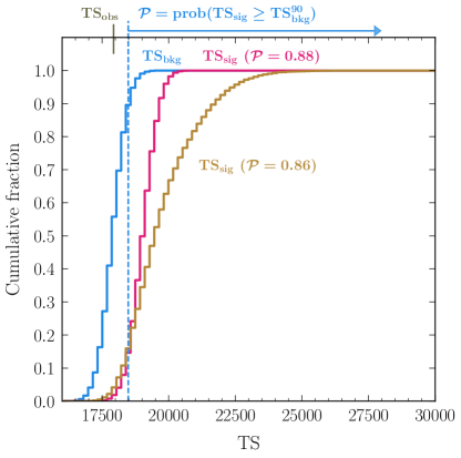
Figure 4: Cumulative TS-value distributions of the data with (labeled with $\rm TS_{sig}$) and without ($\rm TS_{bkg}$) injected signals. Here we use a power-law model with $\gamma=2.0$. We exclude signal hypotheses in which cjSN models lead to excesses of significance compared to the background hypothesis.

IV.1 Neutrino fluence from cjSN

The sensitivity of our analysis to a model strongly depends on its total signal-neutrino flux. For the scenarios of cjSNe, this is closely related to $\mathcal{E}_{\rm CR}$, as the neutrinos are mainly produced through the charged pion decay following the meson production from the $p\gamma$ interactions of accelerated protons in the jet Waxman and Bahcall (1999). For the $k$th data sample, we calculate the number of detected signal neutrino events by the sum of contributions from the individual supernovae, which is

$$N^{k}_{\nu}=\sum^{f_{\rm jet}N^{k}_{\rm SN}}_{j}\int_{E_{\nu}^{\rm min}}^{E_{\nu}^{\rm max}}{\rm d}E_{\nu}A^{k}_{\rm eff}(E_{\nu}|\delta_{{\rm SN}j})\phi_{j}(E_{\nu};\mathcal{E}_{\rm CR})\,,$$ (15)

where, with the flux equally distributed in flavors, the muon-neutrino fluence from a single supernova burst at luminosity distance $d_{j}$ (redshift $z_{j}$) is related to Eq. 1 by

$$\phi_{j}(E_{\nu};\mathcal{E}_{\rm CR})=\frac{(1+z_{j})}{4\pi d_{j}^{2}}\cdot\frac{1}{3}\frac{{\rm d}N_{\nu}(\varepsilon_{\nu};\mathcal{E}_{\rm CR})}{{\rm d}\varepsilon_{\nu}}\,,$$ (16)

the observed neutrino energy is $E_{\nu}=(1+z_{j})^{-1}\varepsilon_{\nu}$, and the Dec of the signal neutrinos is the same as that of their parent supernova, $\delta_{{\rm SN}j}$. $E^{\rm min}_{\nu}$ and $E^{\rm max}_{\nu}$ are determined by the energy range of the accelerated protons at the source.

IV.2 Simulate detected track events

The detected track events from the neutrino events are simulated following the following procedure.

• The arrival time $T_{i}$ is randomly chosen from the signal temporal PDF in Eq. 10.

• The Dec of the neutrino event, $\delta_{i}$, is set to be that of the supernova, $\delta_{{\rm SN}j}$.

• The energy of a detected signal neutrino arriving at Earth, $E^{\rm det}_{\nu i}$, is randomly drawn from the energy spectrum of detected neutrinos; that is, $A^{k}_{\rm eff}(E_{\nu}|\delta_{i})\phi_{j}(E_{\nu})$ in Eq. 15.

• Given the $E^{\rm det}_{\nu i}$ and $\delta_{i}$ of a neutrino event, the proxy energy $E^{\rm prx}_{i}$, angular error, and the point spread function (PSF, the angle between the parent neutrino’s direction and the reconstructed muon direction) of its daughter track event are randomly drawn following the smearing matrix.

• Given the PSF, the angular distance, RA, and Dec of the track are drawn following the signal spatial PDF with $\sigma_{\nu}={\rm PSF}$ in Eq. 12.

V Results and Discussion

In this section, we present our results. In Sec. V.1, we show our single-source and stacking analysis results. Then we show the upper limits on the choked-jet model parameters in Sec. V.2 and their contributions to the diffuse high-energy neutrino flux in Sec. V.3.

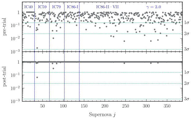
Figure 5: Pre-trial and post-trial p-values of the 386 SNe Ib/c in our sample, given a power-law model with $\gamma=2.0$. The corresponding significance is shown over the y-axis on the right. No significant sources are observed.

V.1 Single-source and stacking analysis results

In our single-source analysis, the pre-trial p-value for individual supernovae ($p^{k}_{{\rm pre},\,j}$) is determined by the probability of finding ${\rm TS}^{k}_{{\rm bkg},\,j}\geq{\rm TS}^{k}_{{\rm obs},\,j}$ in the test statistic distribution under background-only hypothesis. However, a low pre-trial p-value does not necessarily mean a discovery but could be caused by the statistical fluctuations of the background. This can be taken into account by the post-trial p-value, which can be calculated by

$$p^{k}_{{\rm post},\,j}=1-\left(1-p^{k}_{{\rm pre},\,j}\right)^{N^{k}_{\rm SN}}\,.$$ (17)

Figure 5 shows the pre-trial (upper panel) and post-trial (lower panel) p-values of all the SNe Ib/c in our sample, along with the corresponding significance in the unit of standard normal deviations. The results show that none of the supernovae in our sample have significant neutrino emission. The highest pre-trial significance is $\simeq 2.9\sigma$ (SN 2009hy), but its post-trial significance is only $\simeq 1.5\sigma$. Here we only report the p-values based on the power-law spectrum with $\gamma=2.0$, as we find that changing the neutrino spectrum only marginally affects the significance of each source. We provide the p-values for each supernova given all cjSN models at this URL .

Table 1 shows our stacking analysis results. The post-trial p-values are calculated by $p_{\rm post}=1-\left(1-p_{\rm pre}\right)^{6}$, where 6 is the total number of spectra/models we test. The results show that for all the models we consider, the data are consistent with the background-only hypothesis.

Table 1: Pre-trial and post-trial p-values and significance from our stacking analysis for different cjSN models.

Model	$p_{\rm pre}$ (significance)	$p_{\rm post}$ (significance)
$\gamma=2.0$	0.583 (0)	0.995 (0)
$\gamma=2.5$	0.517 (0)	0.987 (0)
$\gamma=3.0$	0.450 (0.1$\sigma$)	0.972 (0)
LLGRB-PE Murase et al. (2006)	0.641 (0)	0.998 (0)
ULGRB-CS Murase and Ioka (2013)	0.613 (0)	0.997 (0)
LPGRB-$\nu$-Attn Carpio and Murase (2020)	0.556 (0)	0.992 (0)

V.2 Stacking constraints on cjSN model parameters

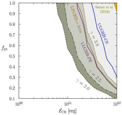
Figure 6: Upper limits on $\mathcal{E}_{\rm CR}$ and $f_{\rm jet}$ for each cjSN model. Also shown in the upper right corner is the existing 90% confidence level limit of $\gamma=2.0$ obtained by previous work Senno et al. (2018) using one year of track events. Realistic models are generally allowed to have larger total energy in cosmic rays, as they are less efficient in producing detectable neutrinos.

Figure 6 shows our upper limits on $\mathcal{E}_{\rm CR}$ and $f_{\rm jet}$ at 90% confidence level for different cjSN models. The parameter space above the curves is excluded. Among all the scenarios we consider, the power-law model with $\gamma=2.0$ have the strongest constraints, because it produces the most signal events in the energy range to which IceCube detectors are most sensitive. For the same reason, power-law models with softer spectra are less constrained, and the limit on the ULGRB-CS model is relatively weak, as it produces the least amount of neutrinos in that energy range.

Our limit on $\mathcal{E}_{\rm CR}$ for the power-law model with $\gamma=2.0$ is stronger than the existing one-year limit in Ref. Senno et al. (2018) by more than an order of magnitude at $f_{\rm jet}=1$. The improvement is expected because our supernovae sample covered by the 10-year IceCube dataset is more than ten times larger than that used in Ref. Senno et al. (2018).

Theoretically, $\mathcal{E}_{\rm CR}$ and to $f_{\rm jet}$ are completely degenerate. In that case, the contours should all follow $\sim 1/\mathcal{E}_{\rm CR}$. However, there is a small deviation at small $f_{\rm jet}$. This is due to the limited number of supernovae in our sample, and for small $f_{\rm jet}$ the uncertainty of our limits on $\mathcal{E}_{\rm CR}$ is larger. Also, it should be noted that our limits are mainly driven by nearby supernovae. Thus, the degeneracy holds when $\sum_{k}f_{\rm jet}(N^{k}_{\rm SN}\cdot f_{\rm nb})>1$, where $f_{\rm nb}$ is the fraction of nearby sources in our samples. During our signal-inject procedure, we find that more than $50\%$ of the signal events are contributed by the supernovae with luminosity distance $d_{j}\lesssim 16\,{\rm Mpc}$, which account for $\lesssim 2\%$ of all the supernovae in our sample, so we set $f_{\rm nb}=0.02$. With $\sum_{k}N^{k}_{\rm SN}=386$ we expect that the limits are obtained for $f_{\rm jet}\gtrsim 0.1$. This implies that with the present supernova sample, the limits on cjSNe models are rather meaningful only if the jets have relatively wide opening angles, $\theta_{j}\gtrsim 0.3$ rad. To test cjSN models with smaller opening angles, e.g., $\theta_{j}\sim 0.1$ rad, better samples with more nearby supernovae are required.

V.3 Upper limits on diffuse neutrino flux

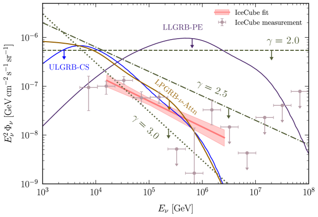
Figure 7: Upper limits on the all-flavor diffuse neutrino flux contributed from each of our cjSN models. The red band corresponds to the IceCube measurement of the all-sky astrophysical neutrino flux and its uncertainties, assuming unbroken single power law: $E_{\nu}^{2}\Phi_{\nu}=\Phi_{0}(E_{\nu}/100\,{\rm TeV})^{2-\gamma}$ with $\Phi_{0}=\left(4.98^{+0.75}_{-0.81}\right)\times 10^{-8}\,{\rm GeV\,cm^{-2}\,s^{-1}\,sr^{-1}}$ and $\gamma=2.53\pm 0.07$ Aartsen et al. (2015a, 2020c). The data points with error bars and the red band represent the best-fit results from the 2010 – 2015 shower data of IceCube Aartsen et al. (2020c). Because of the high local rate density of supernovae, most cjSN models we consider remain viable to explain the diffuse flux of astrophysical neutrinos measured by IceCube.

Now we convert our limits on $\mathcal{E}_{\rm CR}$ and $f_{\rm jet}$ to upper limits on the contribution to diffuse neutrino flux from all the cjSN models. The diffuse flux can be calculated by (e.g., Murase et al. (2016))

$$\Phi_{\nu}(E_{\nu}) =\frac{c}{4\pi H_{0}}\int_{0}^{z_{\rm max}}{\rm d}z\int_{L_{\rm min}}^{L_{\rm max}}{\rm d}L_{\gamma}\hfill$$ (18)

$$\times\frac{{\rm d}\rho(z)/{\rm d}L_{\gamma}}{\sqrt{\Omega_{\Lambda}+\Omega_{\rm m}(1+z)^{3}}}\left.\frac{{\rm d}N_{\nu}(\varepsilon_{\nu};\mathcal{E}_{\rm CR})}{{\rm d}\varepsilon_{\nu}}\right|_{\varepsilon_{\nu}=0.05\varepsilon_{p}}\,,$$

where $\varepsilon_{\nu}\equiv(1+z)E_{\nu}$, ${\rm d}\rho(z)/{\rm d}L_{\gamma}$ is the luminosity function that takes into account the distribution of on-axis choked-jet supernova rate density $\rho(z)=f_{\rm jet}R(z)$ with respect to the observed GRB luminosity, $H_{0}$ is the Hubble constant, and $\{\Omega_{\Lambda},\Omega_{\rm m}\}$ are the cosmological energy density parameters. Combining the above equation with Eq. 1 gives the all-flavor diffuse neutrino flux by Bahcall and Waxman (2001); Murase et al. (2016)

$$E_{\nu}^{2} \Phi_{\nu}(E_{\nu})\sim 7.6\times 10^{-8}\,{\rm GeV\,cm^{-2}\,s^{-1}\,sr^{-1}}$$

$$\times f_{\rm sup}(\varepsilon_{p})\,{\rm min}[1,f_{p\gamma}]\frac{\xi_{z}}{3}\left.\left[\frac{{\mathcal{R}}_{p}(\varepsilon_{p})}{10}\right]^{-1}\right|_{\varepsilon_{p}\sim 20\varepsilon_{\nu}}$$

$$\times\left(\frac{f_{\rm jet}\,\mathcal{E}_{\rm CR}\cdot R_{\rm L}}{10^{51}\,{\rm erg}\cdot 10^{3}\,{\rm Gpc^{-3}\,yr^{-1}}}\right)\,,$$ (19)

where $\xi_{z}$ and $R_{\rm L}\equiv R(0)$ are the redshift evolution factor Waxman and Bahcall (1999); Bahcall and Waxman (2001) and the true local rate density (i.e., volumetric rate) of the supernovae that harbor choked jets (including off-axis ones), respectively. Eq. (19) shows that an upper limit on $f_{\rm jet}\mathcal{E}_{\rm CR}$ directly constrains the maximal neutrino flux we can detect.

Figure 7 shows the upper limits (at $90\%$ confidence level) on the all-flavor diffuse neutrino flux from SNe Ib/c for different cjSN models. The bounds are set via the $\mathcal{E}_{\rm CR}$ limits for $f_{\rm jet}=1$ from Fig. 6. (Note that our limits are sensible for $f_{\rm jet}\gtrsim 0.1$, as discussed below.) To be conservative and consistent with our supernova sample, we take $R_{\rm L}=R_{\rm Ib/c}\sim 2\times 10^{4}\,{\rm Gpc}^{-3}\,{\rm yr}^{-1}$, the local rate density of SNe Ib/c Li et al. (2011); Melinder et al. (2012). We find that most of the models can still explain all the astrophysical neutrino fluxes. In general, the harder the spectrum, the weaker constraints we get. Although we focus on cjSN models, SNe Ib/c may be aided by newborn pulsar winds, which could be emitters of neutrinos in the PeV – EeV range Murase et al. (2009); Fang (2015); Fang et al. (2019). Our analysis results can be applied to such models but the limits are still above the model predictions.

It is worth noting that, although we constrain physical cjSN models motivated by various types of rarer types of supernovae or GRBs, one should not simply downscale our diffuse flux limits by applying the local rate density of rarer source classes to Eq. (19). This is because our SN Ib/c sample does not necessarily include any GRBs or hypernovae. If hypernovae or GRBs (including LL GRBs) only compose a small fraction of the entire supernova sample (i.e., $R_{\rm L}<R_{\rm Ib/c}$), our approach described in Sec. (V.2) may not give a sensible limit. This is the case even if all SNe Ib/c harbor jets (i.e., $R_{\rm L}=R_{\rm Ib/c}$) because only a fraction of them have jets pointing to us. In the current analysis with $\sim 400$ supernovae, we can apply the limits down to $f_{\rm jet}\sim 0.1$ and more supernova samples are necessary to probe cjSN models with smaller jet opening angles. This point is important not to misinterpret the results of the stacking analyses. The choice of the source rate density in the stacking analysis presented here must always be consistent with the sample of sources one takes into account.

V.4 Comparison with prior work

Ref. Necker et al. (2021) performed a similar stacking analysis with cjSNe and 7 years of track events. The result shows that a power-law neutrino spectrum with $\gamma=2.5$ and a similar width of time window contributes no more than $16.4\%$ of the diffuse astrophysical neutrino flux. The constraint is about 10 times stronger than our 10-year limit for $\gamma=2.5$ in Fig. 7, as Ref. Necker et al. (2021) constrained the isotropic equivalent energy to be $\mathcal{E}_{\rm CR}<8\times({\rm limit~{}on~{}total~{}muon~{}neutrino~{}energy})\sim 4\times 10^{49}\,{\rm erg}$, which is also $\sim 10$ times smaller than our result in Section V.2 ($\gamma=2.5$, $f_{\rm jet}=1$: $\mathcal{E}_{\rm CR}<8.3\times 10^{50}\,{\rm erg}$).

A few reasons may cause such discrepancy. First, Ref. Necker et al. (2021) analyzed a subsample of 19 nearby supernovae that accounts for 70% the total neutrino flux. We find that, for all models, our limits on $\mathcal{E}_{\rm CR}$ in Fig. 6 (with $f_{\rm jet}=1$) and the diffuse neutrino flux in Fig. 7 could be stronger by a factor of $3$ – $4$ if we analyze the subsample that dominates the total neutrino flux because the total background would be reduced. We emphasize that, for our main results, we do not select any subsamples in the analyses, so our limits are regarded as robust and ‘conservative’ constraints on cjSN models. Importantly, even if all supernovae harbor jets, only a fraction ($f_{\rm jet}$) of them would point to us. In reality, the viewing angle of choked jets can be small so that $f_{\rm jet}\ll 1$. We caution that the stacking analysis with a small subsample will greatly decrease the sensitivity for $f_{\rm jet}\ll 1$. If none of the on-axis events are included in the nearby sample, sensible constraints cannot be placed as the viewing angle of choked jets is unknown.

Second, there is an important difference between the source catalog of Ref. Necker et al. (2021) and ours: their catalog includes some nearby Type IIb supernovae (e.g., SN 2011dh), while we only include Type Ib/c supernovae as cjSNe are typically expected to be detected as these types. We find that the large flux produced by the additional SNe IIb would affect the final constraints by a factor of $\sim 2$.

Third, Ref. Necker et al. (2021) constructed signal energy PDFs through the smearing matrices from IceCube’s internal Monte-Carlo simulations, which are different from the publicly released smearing matrices we use and may also lead to an improvement in the final sensitivity.

Finally, the likelihood formalism used in Ref. Necker et al. (2021) is slightly different from ours. We use the same formalism as IceCube’s search for neutrino emission from transient sources like GRBs Abbasi et al. (2010, 2009); Aartsen et al. (2015b, 2016, 2017a) and fast-radio bursts Aartsen et al. (2018c); Fahey et al. (2018, 2018); Aartsen et al. (2020d); Kheirandish et al. (2021), which includes a Poisson weighting factor (Eq. (4)). Ref. Necker et al. (2021) used a different weighting method, as some of their analyses have much longer time windows (up to 1000 days).

Furthermore, we note that the constraints with steep spectral indices such as $\gamma=2.5$ lead to aggressive limits on the contribution to the diffuse neutrino flux. As shown in Fig. 7, the limits for harder indices are weaker for neutrinos at energies above $\sim 30$ TeV. Also, models with steep spectra down to TeV energies cannot make a significant contribution to the diffuse flux in light of energetics of GRBs and SNe, and most of the viable models in the literature have a low-energy break or cutoff. Ref. Necker et al. (2021) did not provide the constraints on models with harder indices or more realistic neutrino spectra, and their limits are used for constraining models with much caution.

All in all, our results are complementary to Ref. Necker et al. (2021) in various aspects. We focus on setting robust constraints on various physical neutrino emission models of cjSNe with $f_{\rm jet}\leq 1$ using SNe Ib/c, while Ref. Necker et al. (2021) puts constraints on power-law models with $f_{\rm jet}=1$ using both SNe Ib/c and SNe IIb, but we stress that these limits should be interpreted with much caution from the theoretical perspectives.

VI Conclusions

The detection of TeV – PeV astrophysical neutrino flux by IceCube is a breakthrough in neutrino physics, astrophysics, and multimessenger astronomy. These neutrinos are unique probes of neutrino physics at high energies in the standard model Glashow (1960); Seckel (1998); Alikhanov (2016); Aartsen et al. (2017b); Bustamante and Connolly (2019); Zhou and Beacom (2020a, b); Abbasi et al. (2020); Aartsen et al. (2021a); Zhou and Beacom (2022) and beyond Lipari (2001); Cornet et al. (2001); Beacom et al. (2003, 2007); Yuksel et al. (2007); Murase and Beacom (2012); Feldstein et al. (2013); Esmaili and Serpico (2013); Murase et al. (2015); Shoemaker and Murase (2016); Bustamante et al. (2017); Aartsen et al. (2017c); Coloma et al. (2017); Denton and Tamborra (2018); Aartsen et al. (2018d); Argüelles et al. (2021); Esteban et al. (2021). They also directly probe the interior of astrophysical dense environments opaque to photons and will cast light on the long-standing problems: the origin of HE cosmic rays and their acceleration mechanisms. To fully exploit the exclusive opportunities brought by HE astrophysical neutrinos, searching for and studying their sources are the essential steps.

Previous studies indicated that most astrophysical neutrino sources should be optically thick to gamma rays Murase et al. (2016). Among promising gamma-ray dark candidates, core-collapse supernovae with jets choked by surrounding materials are especially interesting Murase and Ioka (2013); Tamborra and Ando (2016); Senno et al. (2016), as they 1) naturally explain the potential connections between SNe Ib/c, hypernovae, and classical, LL, and UL GRBs, and 2) are efficient in producing HE astrophysical neutrinos.

In this paper, we studied whether cjSNe can be the dominant source contributing to the diffuse astrophysical neutrinos detected by IceCube. We used the unbinned-maximum-likelihood method to search for the associations between IceCube neutrinos and SNe Ib/c. Compared to existing searches, our analysis takes advantage of 10 years of IceCube neutrino data. We also collected SNe Ib/c from publicly available supernova catalogs covering the same period. Importantly, for the first time, we looked for the neutrino signals of physical cjSN models in IceCube data. These models take into account a variety of time-dependent cooling processes for cosmic rays and mesons in LP GRBs, which are well-motivated but have never been constrained by data.

For all the cjSN models we considered, our single-source analysis (Fig. 5) and stacking analysis (Table 1) found no significant correlation between the muon-track events and any SNe Ib/c in our source sample with respect to the backgrounds. Thus, we put upper limits on, $\mathcal{E}_{\rm CR}$, the total energy budget of cosmic rays and, $f_{\rm jet}$, the fraction of SNe Ib/c that has choked jets pointing to us for different cjSN models. Our 10-year limit improves the prior 1-year limit in Ref. Senno et al. (2018) by more than an order of magnitude (Fig. 6). Moreover, the limits of both parameters are generally sensitive to the efficiency of a cjSN model in producing detectable neutrinos by IceCube (see the right panel of Fig. 3), which can vary by a factor up to $\sim 5$ among the models we consider.

We set the corresponding upper limits of the cumulative astrophysical neutrino fluxes contributed by all SNe Ib/c for each model (Fig. 7). In contrast to strongly-constrained transient neutrino sources such as classical GRBs Abbasi et al. (2010, 2009); Aartsen et al. (2015b, 2016, 2017a), jetted TDEs Stein (2020), gamma-ray blazars Aartsen et al. (2017d); Hooper et al. (2019); Yuan et al. (2020); Luo and Zhang (2020); Smith et al. (2021), and radio-loud AGN Plavin et al. (2020, 2021); Zhou et al. (2021), SNe Ib/c have a much higher volumetric rate (see Table 1 of Ref. Murase and Bartos (2019)), so they could potentially make a large contribution to HE neutrino fluxes whether they have choked jets or not.

Future prospects of testing cjSNe as neutrino sources are very promising. From Fig. 7, we clearly see that most of our conservative limits obtained from 10 years of data are close to the measured astrophysical neutrino flux in IceCube. Given that IceCube-Gen2 Aartsen et al. (2021b) will be at least 5 times more sensitive than IceCube, IceCube-Gen2 will effectively strengthen our stacking limits and critically constrain most cjSN models with just 2 years of operation. Additionally, there will be much more high-quality data from other observatories such as KM3NeT Adrian-Martinez et al. (2016), Baikal-GVD Avrorin et al. (2018), P-ONE Agostini et al. (2020), and TRIDENT Ye et al. (2022), which are sensitive to different parts of the sky. Importantly, the Vera C. Rubin Observatory’s upcoming Legacy Survey of Space and Time (LSST) Abell et al. (2009); Ivezić et al. (2019) will increase the detection rate of supernovae by more than an order of magnitude ($>10^{5}$ core-collapse supernovae per year Lien and Fields (2009); Lien et al. (2010)). The improvement of the redshift completeness of nearby supernova samples at low redshift ($z\lesssim 10^{-2}$) will dramatically boost the sensitivities of future stacking analyses; furthermore, an increase of the observed supernovae at higher redshift will be beneficial to constraining the cjSN models with $f_{\rm jet}\ll 0.1$. This is crucial because the typical beaming factor of GRB jets is believed to be $f_{\rm jet}\sim 0.01$. Together, core-collapse supernovae with choked jets have reached the fork of being discovered or ruled out as dominant neutrino sources. Our insights into the interrelationship between the most elusive high-energy particles and the stellar explosions within dense environments will drastically grow in the near future.

References

- Aartsen et al. (2013a) M. G. Aartsen et al. (IceCube), “First observation of PeV-energy neutrinos with IceCube,” Phys. Rev. Lett. 111, 021103 (2013a), arXiv:1304.5356 [astro-ph.HE] .
- Aartsen et al. (2013b) M. G. Aartsen et al. (IceCube), “Evidence for High-Energy Extraterrestrial Neutrinos at the IceCube Detector,” Science 342, 1242856 (2013b), arXiv:1311.5238 [astro-ph.HE] .
- Paczynski and Xu (1994) B. Paczynski and G. H. Xu, “Neutrino bursts from gamma-ray bursts,” Astrophys. J. 427, 708–713 (1994).
- Waxman and Bahcall (1997) Eli Waxman and John N. Bahcall, “High-energy neutrinos from cosmological gamma-ray burst fireballs,” Phys. Rev. Lett. 78, 2292–2295 (1997), arXiv:astro-ph/9701231 [astro-ph] .
- Dermer and Atoyan (2003) Charles D. Dermer and Armen Atoyan, “High energy neutrinos from gamma-ray bursts,” Phys. Rev. Lett. 91, 071102 (2003), arXiv:astro-ph/0301030 .
- Kimura (2022) Shigeo S. Kimura, “Neutrinos from Gamma-ray Bursts,” (2022), arXiv:2202.06480 [astro-ph.HE] .
- Berezinsky (1977) V. S. Berezinsky, in Proc. of Neutrinos-1977, Elbros. (1977).
- Eichler (1979) D. Eichler, “HIGH-ENERGY NEUTRINO ASTRONOMY: A PROBE OF GALACTIC NUCLEI?” Astrophys. J. 232, 106–112 (1979).
- Stecker et al. (1991) F. W. Stecker, C. Done, M. H. Salamon, and P. Sommers, “High-energy neutrinos from active galactic nuclei,” Phys. Rev. Lett. 66, 2697–2700 (1991).
- Murase (2017) Kohta Murase, “Active Galactic Nuclei as High-Energy Neutrino Sources,” in Neutrino Astronomy: Current Status, Future Prospects, edited by Thomas Gaisser and Albrecht Karle (2017) pp. 15–31, arXiv:1511.01590 [astro-ph.HE] .
- Murase et al. (2011) Kohta Murase, Todd A. Thompson, Brian C. Lacki, and John F. Beacom, “New Class of High-Energy Transients from Crashes of Supernova Ejecta with Massive Circumstellar Material Shells,” Phys. Rev. D84, 043003 (2011), arXiv:1012.2834 [astro-ph.HE] .
- Murase (2018) Kohta Murase, “New Prospects for Detecting High-Energy Neutrinos from Nearby Supernovae,” Phys. Rev. D 97, 081301 (2018), arXiv:1705.04750 [astro-ph.HE] .
- Murase (2008) Kohta Murase, “Astrophysical high-energy neutrinos and gamma-ray bursts,” AIP Conf. Proc. 1065, 201–206 (2008).
- Wang and Liu (2016) Xiang-Yu Wang and Ruo-Yu Liu, “Tidal disruption jets of supermassive black holes as hidden sources of cosmic rays: explaining the IceCube TeV-PeV neutrinos,” Phys. Rev. D 93, 083005 (2016), arXiv:1512.08596 [astro-ph.HE] .
- Dai and Fang (2017) Lixin Dai and Ke Fang, “Can tidal disruption events produce the IceCube neutrinos?” Mon. Not. Roy. Astron. Soc. 469, 1354–1359 (2017), arXiv:1612.00011 [astro-ph.HE] .
- Senno et al. (2017) Nicholas Senno, Kohta Murase, and Peter Meszaros, “High-energy Neutrino Flares from X-Ray Bright and Dark Tidal Disruption Events,” Astrophys. J. 838, 3 (2017), arXiv:1612.00918 [astro-ph.HE] .
- Lunardini and Winter (2017) Cecilia Lunardini and Walter Winter, “High Energy Neutrinos from the Tidal Disruption of Stars,” Phys. Rev. D 95, 123001 (2017), arXiv:1612.03160 [astro-ph.HE] .
- Aartsen et al. (2018a) M. G. Aartsen et al. (IceCube, Fermi-LAT, MAGIC, AGILE, ASAS-SN, HAWC, H.E.S.S., INTEGRAL, Kanata, Kiso, Kapteyn, Liverpool Telescope, Subaru, Swift NuSTAR, VERITAS, VLA/17B-403), “Multimessenger observations of a flaring blazar coincident with high-energy neutrino IceCube-170922A,” Science 361, eaat1378 (2018a), arXiv:1807.08816 [astro-ph.HE] .
- Aartsen et al. (2018b) M. G. Aartsen et al. (IceCube), “Neutrino emission from the direction of the blazar TXS 0506+056 prior to the IceCube-170922A alert,” Science 361, 147–151 (2018b), arXiv:1807.08794 [astro-ph.HE] .
- Aartsen et al. (2020a) M. G. Aartsen et al. (IceCube), “Time-Integrated Neutrino Source Searches with 10 Years of IceCube Data,” Phys. Rev. Lett. 124, 051103 (2020a), arXiv:1910.08488 [astro-ph.HE] .
- Stein et al. (2021) Robert Stein et al., “A tidal disruption event coincident with a high-energy neutrino,” Nature Astron. 5, 510–518 (2021), arXiv:2005.05340 [astro-ph.HE] .
- Reusch et al. (2022) Simeon Reusch et al., “Candidate Tidal Disruption Event AT2019fdr Coincident with a High-Energy Neutrino,” Phys. Rev. Lett. 128, 221101 (2022), arXiv:2111.09390 [astro-ph.HE] .
- van Velzen et al. (2021) S. van Velzen et al., “Establishing accretion flares from massive black holes as a major source of high-energy neutrinos,” (2021), arXiv:2111.09391 [astro-ph.HE] .
- Abbasi et al. (2022) R. Abbasi et al. (IceCube), “Search for neutrino emission from cores of active galactic nuclei,” Phys. Rev. D 106, 022005 (2022), arXiv:2111.10169 [astro-ph.HE] .
- Ackermann et al. (2015) M. Ackermann et al. (Fermi-LAT), “The spectrum of isotropic diffuse gamma-ray emission between 100 MeV and 820 GeV,” Astrophys. J. 799, 86 (2015), arXiv:1410.3696 [astro-ph.HE] .
- Murase et al. (2013) Kohta Murase, Markus Ahlers, and Brian C. Lacki, “Testing the Hadronuclear Origin of PeV Neutrinos Observed with IceCube,” Phys. Rev. D88, 121301 (2013), arXiv:1306.3417 [astro-ph.HE] .
- Murase et al. (2016) Kohta Murase, Dafne Guetta, and Markus Ahlers, “Hidden Cosmic-Ray Accelerators as an Origin of TeV-PeV Cosmic Neutrinos,” Phys. Rev. Lett. 116, 071101 (2016), arXiv:1509.00805 [astro-ph.HE] .
- Capanema et al. (2020) Antonio Capanema, Arman Esmaili, and Kohta Murase, “New constraints on the origin of medium-energy neutrinos observed by IceCube,” Phys. Rev. D101, 103012 (2020), arXiv:2002.07192 [hep-ph] .
- Capanema et al. (2021) Antonio Capanema, Arman Esmaili, and Pasquale Dario Serpico, “Where do IceCube neutrinos come from? Hints from the diffuse gamma-ray flux,” JCAP 2102, 037 (2021), arXiv:2007.07911 [hep-ph] .
- Fang et al. (2022) Ke Fang, John S. Gallagher, and Francis Halzen, “The TeV Diffuse Cosmic Neutrino Spectrum and the Nature of Astrophysical Neutrino Sources,” Astrophys. J. 933, 190 (2022), arXiv:2205.03740 [astro-ph.HE] .
- Fasano et al. (2021) Michela Fasano, Silvia Celli, Dafne Guetta, Antonio Capone, Angela Zegarelli, and Irene Di Palma, “Estimating the neutrino flux from choked gamma-ray bursts,” JCAP 09, 044 (2021), arXiv:2101.03502 [astro-ph.HE] .
- Meszaros and Waxman (2001) Peter Meszaros and Eli Waxman, “TeV neutrinos from successful and choked gamma-ray bursts,” Phys. Rev. Lett. 87, 171102 (2001), arXiv:astro-ph/0103275 .
- Razzaque et al. (2004) Soebur Razzaque, Peter Meszaros, and Eli Waxman, “TeV neutrinos from core collapse supernovae and hypernovae,” Phys. Rev. Lett. 93, 181101 (2004), [Erratum: Phys.Rev.Lett. 94, 109903 (2005)], arXiv:astro-ph/0407064 .
- Razzaque et al. (2005) Soebur Razzaque, Peter Meszaros, and Eli Waxman, “High energy neutrinos from a slow jet model of core collapse supernovae,” Mod. Phys. Lett. A 20, 2351–2368 (2005), arXiv:astro-ph/0509729 .
- Ando and Beacom (2005) Shin’ichiro Ando and John F. Beacom, “Revealing the supernova-gamma-ray burst connection with TeV neutrinos,” Phys. Rev. Lett. 95, 061103 (2005), arXiv:astro-ph/0502521 .
- Murase and Ioka (2013) Kohta Murase and Kunihito Ioka, “TeV – PeV Neutrinos from Low-Power Gamma-Ray Burst Jets inside Stars,” Phys. Rev. Lett. 111, 121102 (2013), arXiv:1306.2274 [astro-ph.HE] .
- He et al. (2018) Hao-Ning He, Alexander Kusenko, Shigehiro Nagataki, Yi-Zhong Fan, and Da-Ming Wei, “Neutrinos from Choked Jets Accompanied by Type-II Supernovae,” Astrophys. J. 856, 119 (2018), arXiv:1803.07478 [astro-ph.HE] .
- Tamborra and Ando (2016) Irene Tamborra and Shin’ichiro Ando, “Inspecting the supernova–gamma-ray-burst connection with high-energy neutrinos,” Phys. Rev. D 93, 053010 (2016), arXiv:1512.01559 [astro-ph.HE] .
- Senno et al. (2016) Nicholas Senno, Kohta Murase, and Peter Meszaros, “Choked Jets and Low-Luminosity Gamma-Ray Bursts as Hidden Neutrino Sources,” Phys. Rev. D 93, 083003 (2016), arXiv:1512.08513 [astro-ph.HE] .
- Guetta et al. (2020) Dafne Guetta, Roi Rahin, Imre Bartos, and Massimo Della Valle, “Constraining the fraction of core-collapse supernovae harbouring choked jets with high-energy neutrinos,” Mon. Not. Roy. Astron. Soc. 492, 843–847 (2020), arXiv:1906.07399 [astro-ph.HE] .
- Carpio and Murase (2020) Jose Carpio and Kohta Murase, “Oscillation of high-energy neutrinos from choked jets in stellar and merger ejecta,” Phys. Rev. D 101, 123002 (2020), arXiv:2002.10575 [astro-ph.HE] .
- Nakar (2015) Ehud Nakar, “A unified picture for low-luminosity and long gamma-ray bursts based on the extended progenitor of llgrb 060218/SN 2006aj,” Astrophys. J. 807, 172 (2015), arXiv:1503.00441 [astro-ph.HE] .
- Galama et al. (1998) T. J. Galama et al., “An unusual supernova in the error box of the -ray burst of 25 April 1998,” Nature (London) 395, 670–672 (1998), arXiv:astro-ph/9806175 [astro-ph] .
- Hjorth et al. (2003) Jens Hjorth et al., “A Very energetic supernova associated with the gamma-ray burst of 29 March 2003,” Nature 423, 847–850 (2003), arXiv:astro-ph/0306347 .
- Stanek et al. (2003) Krzysztof Z. Stanek et al., “Spectroscopic discovery of the supernova 2003dh associated with GRB 030329,” Astrophys. J. Lett. 591, L17–L20 (2003), arXiv:astro-ph/0304173 .
- Modjaz et al. (2016) Maryam Modjaz, Yuqian. Q. Liu, Federica B. Bianco, and Or Graur, “The Spectral SN-GRB Connection: Systematic Spectral Comparisons between Type Ic Supernovae, and broad-lined Type Ic Supernovae with and without Gamma-Ray Bursts,” Astrophys. J. 832, 108 (2016), arXiv:1509.07124 [astro-ph.HE] .
- Abbasi et al. (2011) R. Abbasi et al. (IceCube), “Constraints on high-energy neutrino emission from SN 2008D,” Astron. Astrophys. 527, A28 (2011), arXiv:1101.3942 [astro-ph.HE] .
- Abbasi et al. (2012) R. Abbasi et al. (IceCube, ROTSE), “Searching for soft relativistic jets in Core-collapse Supernovae with the IceCube Optical Follow-up Program,” Astron. Astrophys. 539, A60 (2012), arXiv:1111.7030 [astro-ph.HE] .
- Senno et al. (2018) Nicholas Senno, Kohta Murase, and Peter Mészáros, “Constraining high-energy neutrino emission from choked jets in stripped-envelope supernovae,” JCAP 01, 025 (2018), arXiv:1706.02175 [astro-ph.HE] .
- Esmaili and Murase (2018) Arman Esmaili and Kohta Murase, “Constraining high-energy neutrinos from choked-jet supernovae with IceCube high-energy starting events,” JCAP 1812, 008 (2018), arXiv:1809.09610 [hep-ph] .
- Necker et al. (2021) Jannis Necker et al. (IceCube), “Searching for High-Energy Neutrinos from Core-Collapse Supernovae with IceCube,” PoS ICRC2021, 1116 (2021), arXiv:2107.09317 [astro-ph.HE] .
- Abbasi et al. (2021a) R. Abbasi et al. (IceCube), “IceCube Data for Neutrino Point-Source Searches Years 2008-2018,” (2021a), 10.21234/CPKQ-K003, arXiv:2101.09836 [astro-ph.HE] .
- (53) IceCube Collaboration (2021), “All-sky point-source IceCube data: years 2008-2018. Dataset. ,” 10.21234/sxvs-mt83.
- Achterberg et al. (2006) A. Achterberg et al. (IceCube), “First Year Performance of The IceCube Neutrino Telescope,” Astropart. Phys. 26, 155–173 (2006), arXiv:astro-ph/0604450 [astro-ph] .
- (55) https://icecube.wisc.edu/.
- (56) https://www.icrc2019.org/uploads/1/1/9/0/119067782/nu4b_schneider.pdf.
- Aartsen et al. (2020b) M. G. Aartsen et al. (IceCube), “Time-Integrated Neutrino Source Searches with 10 Years of IceCube Data,” Phys. Rev. Lett. 124, 051103 (2020b), arXiv:1910.08488 [astro-ph.HE] .
- Zhou et al. (2021) Bei Zhou, Marc Kamionkowski, and Yun-feng Liang, “Search for High-Energy Neutrino Emission from Radio-Bright AGN,” Phys. Rev. D 103, 123018 (2021), arXiv:2103.12813 [astro-ph.HE] .
- Zhou and Beacom (2022) Bei Zhou and John F. Beacom, “Dimuons in neutrino telescopes: New predictions and first search in IceCube,” Phys. Rev. D 105, 093005 (2022), arXiv:2110.02974 [hep-ph] .
- Guillochon et al. (2017) James Guillochon, Jerod Parrent, Luke Zoltan Kelley, and Raffaella Margutti, “An Open Catalog for Supernova Data,” Astrophys. J. 835, 64 (2017), arXiv:1605.01054 [astro-ph.SR] .
- Yaron and Gal-Yam (2012) Ofer Yaron and Avishay Gal-Yam, “WISeREP - An Interactive Supernova Data Repository,” Publ. Astron. Soc. Pac. 124, 668 (2012), arXiv:1204.1891 [astro-ph.IM] .
- Holoien et al. (2017a) T. W. S. Holoien et al., “The ASAS-SN bright supernova catalogue – I. 2013–2014,” Mon. Not. Roy. Astron. Soc. 464, 2672–2686 (2017a), arXiv:1604.00396 [astro-ph.HE] .
- Holoien et al. (2017b) T. W. S. Holoien et al., “The ASAS-SN bright supernova catalogue – II. 2015,” Mon. Not. Roy. Astron. Soc. 467, 1098–1111 (2017b), arXiv:1610.03061 [astro-ph.HE] .
- Holoien et al. (2017c) T. W. S. Holoien et al., “The ASAS-SN bright supernova catalogue – III. 2016,” Mon. Not. Roy. Astron. Soc. 471, 4966–4981 (2017c), arXiv:1704.02320 [astro-ph.HE] .
- Holoien et al. (2019) T. W. S. Holoien et al., “The ASAS-SN bright supernova catalogue – IV. 2017,” Mon. Not. Roy. Astron. Soc. 484, 1899–1911 (2019), arXiv:1811.08904 [astro-ph.HE] .
- (66) https://www.rochesterastronomy.org/snimages/.
- Gal-Yam et al. (2013) Avishay Gal-Yam, P. A. Mazzali, I. Manulis, and D. Bishop, “Supernova discoveries 2010–2011: Statistics and trends,” Publications of the Astronomical Society of the Pacific 125, 749–752 (2013).
- Murase et al. (2006) Kohta Murase, Kunihito Ioka, Shigehiro Nagataki, and Takashi Nakamura, “High Energy Neutrinos and Cosmic-Rays from Low-Luminosity Gamma-Ray Bursts?” Astrophys. J. Lett. 651, L5–L8 (2006), arXiv:astro-ph/0607104 .
- Waxman and Bahcall (1999) Eli Waxman and John N. Bahcall, “High-energy neutrinos from astrophysical sources: An Upper bound,” Phys. Rev. D 59, 023002 (1999), arXiv:hep-ph/9807282 .
- Murase and Bartos (2019) Kohta Murase and Imre Bartos, “High-Energy Multimessenger Transient Astrophysics,” Ann. Rev. Nucl. Part. Sci. 69, 477–506 (2019), arXiv:1907.12506 [astro-ph.HE] .
- Waxman (1995) Eli Waxman, “Cosmological origin for cosmic rays above eV,” Astrophys. J. Lett. 452, L1–L4 (1995), arXiv:astro-ph/9508037 .
- Fermi (1949) Enrico Fermi, “On the Origin of the Cosmic Radiation,” Phys. Rev. 75, 1169–1174 (1949).
- Stettner (2020) J. Stettner (IceCube), “Measurement of the Diffuse Astrophysical Muon-Neutrino Spectrum with Ten Years of IceCube Data,” PoS ICRC2019, 1017 (2020), arXiv:1908.09551 [astro-ph.HE] .
- Aartsen et al. (2015a) M. G. Aartsen et al. (IceCube), “A combined maximum-likelihood analysis of the high-energy astrophysical neutrino flux measured with IceCube,” Astrophys. J. 809, 98 (2015a), arXiv:1507.03991 [astro-ph.HE] .
- Aartsen et al. (2020c) M. G. Aartsen et al. (IceCube), “Characteristics of the diffuse astrophysical electron and tau neutrino flux with six years of IceCube high energy cascade data,” Phys. Rev. Lett. 125, 121104 (2020c), arXiv:2001.09520 [astro-ph.HE] .
- Abbasi et al. (2021b) R. Abbasi et al. (IceCube), “The IceCube high-energy starting event sample: Description and flux characterization with 7.5 years of data,” Phys. Rev. D 104, 022002 (2021b), arXiv:2011.03545 [astro-ph.HE] .
- Abbasi et al. (2010) R. Abbasi et al. (IceCube), “Search for muon neutrinos from Gamma-Ray Bursts with the IceCube neutrino telescope,” Astrophys. J. 710, 346–359 (2010), arXiv:0907.2227 [astro-ph.HE] .
- Abbasi et al. (2009) R. Abbasi et al. (IceCube), “Search for high-energy muon neutrinos from the ’naked-eye’ GRB 080319B with the IceCube neutrino telescope,” Astrophys. J. 701, 1721–1731 (2009), [Erratum: Astrophys.J. 708, 911–912 (2010)], arXiv:0902.0131 [astro-ph.HE] .
- Aartsen et al. (2015b) M. G. Aartsen et al. (IceCube), “Search for Prompt Neutrino Emission from Gamma-Ray Bursts with IceCube,” Astrophys. J. Lett. 805, L5 (2015b), arXiv:1412.6510 [astro-ph.HE] .
- Aartsen et al. (2016) M. G. Aartsen et al. (IceCube), “An All-Sky Search for Three Flavors of Neutrinos from Gamma-Ray Bursts with the IceCube Neutrino Observatory,” Astrophys. J. 824, 115 (2016), arXiv:1601.06484 [astro-ph.HE] .
- Aartsen et al. (2017a) M. G. Aartsen et al. (IceCube), “Extending the search for muon neutrinos coincident with gamma-ray bursts in IceCube data,” Astrophys. J. 843, 112 (2017a), arXiv:1702.06868 [astro-ph.HE] .
- Aartsen et al. (2018c) M. G. Aartsen et al. (IceCube), “A Search for Neutrino Emission from Fast Radio Bursts with Six Years of IceCube Data,” Astrophys. J. 857, 117 (2018c), arXiv:1712.06277 [astro-ph.HE] .
- Fahey et al. (2018) Sam Fahey, Justin Vandenbroucke, and Donglian Xu (IceCube), “Search for High-Energy Neutrino Emission from Fast Radio Bursts,” PoS ICRC2017, 980 (2018).
- Aartsen et al. (2020d) M. G. Aartsen et al. (IceCube), “A Search for MeV to TeV Neutrinos from Fast Radio Bursts with IceCube,” Astrophys. J. 890, 111 (2020d), arXiv:1908.09997 [astro-ph.HE] .
- Kheirandish et al. (2021) Ali Kheirandish, Alex Pizzuto, and Justin Vandenbroucke (IceCube), “Searches for neutrinos from fast radio bursts with IceCube,” PoS ICRC2019, 982 (2021), arXiv:1909.00078 [astro-ph.HE] .
- Thrane et al. (2009) E. Thrane et al. (Super-Kamiokande), “Search for Astrophysical Neutrino Point Sources at Super-Kamiokande,” Astrophys. J. 704, 503–512 (2009), arXiv:0907.1594 [astro-ph.HE] .
- Cano et al. (2017) Zach Cano, Shan-Qin Wang, Zi-Gao Dai, and Xue-Feng Wu, “The Observer’s Guide to the Gamma-Ray Burst Supernova Connection,” Adv. Astron. 2017, 8929054 (2017), arXiv:1604.03549 [astro-ph.HE] .
- Fisher (1953) Ronald Fisher, “Dispersion on a sphere,” Proceedings of the Royal Society of London. Series A, Mathematical and Physical Sciences 217, 295–305 (1953).
- Bingham and Mardia (1978) Christopher Bingham and K. V. Mardia, “A small circle distribution on the sphere,” Biometrika 65, 379–389 (1978).
- Kent (1982) John T. Kent, “The fisher-bingham distribution on the sphere,” Journal of the Royal Statistical Society. Series B (Methodological) 44, 71–80 (1982).
- Bahcall and Waxman (2001) John N. Bahcall and Eli Waxman, “High-energy astrophysical neutrinos: The Upper bound is robust,” Phys. Rev. D 64, 023002 (2001), arXiv:hep-ph/9902383 .
- Li et al. (2011) Weidong Li et al., “Nearby Supernova Rates from the Lick Observatory Supernova Search. II. The Observed Luminosity Functions and Fractions of Supernovae in a Complete Sample,” Mon. Not. Roy. Astron. Soc. 412, 1441 (2011), arXiv:1006.4612 [astro-ph.SR] .
- Melinder et al. (2012) J. Melinder, T. Dahlen, L. Mencia Trinchant, G. Ostlin, S. Mattila, J. Sollerman, C. Fransson, M. Hayes, E. Kankare, and S. Nasoudi-Shoar, “The Rate of Supernovae at Redshift 0.1-1.0 - the Stockholm VIMOS Supernova Survey IV,” Astron. Astrophys. 545, A96 (2012), arXiv:1206.6897 [astro-ph.CO] .
- Murase et al. (2009) Kohta Murase, Peter Meszaros, and Bing Zhang, “Probing the birth of fast rotating magnetars through high-energy neutrinos,” Phys. Rev. D 79, 103001 (2009), arXiv:0904.2509 [astro-ph.HE] .
- Fang (2015) Ke Fang, “High-Energy Neutrino Signatures of Newborn Pulsars In the Local Universe,” JCAP 06, 004 (2015), arXiv:1411.2174 [astro-ph.HE] .
- Fang et al. (2019) Ke Fang, Brian D. Metzger, Kohta Murase, Imre Bartos, and Kumiko Kotera, “Multimessenger Implications of AT2018cow: High-energy Cosmic-Ray and Neutrino Emissions from Magnetar-powered Superluminous Transients,” Astrophys. J. 878, 34 (2019), arXiv:1812.11673 [astro-ph.HE] .
- Glashow (1960) Sheldon L. Glashow, “Resonant Scattering of Antineutrinos,” Phys. Rev. 118, 316–317 (1960).
- Seckel (1998) D. Seckel, “Neutrino photon reactions in astrophysics and cosmology,” Phys. Rev. Lett. 80, 900–903 (1998), arXiv:hep-ph/9709290 [hep-ph] .
- Alikhanov (2016) I. Alikhanov, “Hidden Glashow resonance in neutrino-nucleus collisions,” Phys. Lett. B756, 247–253 (2016), arXiv:1503.08817 [hep-ph] .
- Aartsen et al. (2017b) M. G. Aartsen et al. (IceCube), “Measurement of the multi-TeV neutrino cross section with IceCube using Earth absorption,” Nature 551, 596–600 (2017b), arXiv:1711.08119 [hep-ex] .
- Bustamante and Connolly (2019) Mauricio Bustamante and Amy Connolly, “Extracting the Energy-Dependent Neutrino-Nucleon Cross Section above 10 TeV Using IceCube Showers,” Phys. Rev. Lett. 122, 041101 (2019), arXiv:1711.11043 [astro-ph.HE] .
- Zhou and Beacom (2020a) Bei Zhou and John F. Beacom, “Neutrino-nucleus cross sections for W-boson and trident production,” Phys. Rev. D 101, 036011 (2020a), arXiv:1910.08090 [hep-ph] .
- Zhou and Beacom (2020b) Bei Zhou and John F. Beacom, “W-boson and trident production in TeV–PeV neutrino observatories,” Phys. Rev. D 101, 036010 (2020b), arXiv:1910.10720 [hep-ph] .
- Abbasi et al. (2020) R. Abbasi et al. (IceCube), “Measurement of the high-energy all-flavor neutrino-nucleon cross section with IceCube,” (2020), arXiv:2011.03560 [hep-ex] .
- Aartsen et al. (2021a) M. G. Aartsen et al. (IceCube), “Detection of a particle shower at the Glashow resonance with IceCube,” Nature 591, 220–224 (2021a), [Erratum: Nature 592, E11 (2021)].
- Lipari (2001) Paolo Lipari, “CP violation effects and high-energy neutrinos,” Phys. Rev. D64, 033002 (2001), arXiv:hep-ph/0102046 [hep-ph] .
- Cornet et al. (2001) F. Cornet, Jose I. Illana, and M. Masip, “TeV strings and the neutrino nucleon cross-section at ultrahigh-energies,” Phys. Rev. Lett. 86, 4235–4238 (2001), arXiv:hep-ph/0102065 [hep-ph] .
- Beacom et al. (2003) John F. Beacom, Nicole F. Bell, Dan Hooper, Sandip Pakvasa, and Thomas J. Weiler, “Decay of High-Energy Astrophysical Neutrinos,” Phys. Rev. Lett. 90, 181301 (2003), arXiv:hep-ph/0211305 [hep-ph] .
- Beacom et al. (2007) John F. Beacom, Nicole F. Bell, and Gregory D. Mack, “General Upper Bound on the Dark Matter Total Annihilation Cross Section,” Phys. Rev. Lett. 99, 231301 (2007), arXiv:astro-ph/0608090 .
- Yuksel et al. (2007) Hasan Yuksel, Shunsaku Horiuchi, John F. Beacom, and Shin’ichiro Ando, “Neutrino Constraints on the Dark Matter Total Annihilation Cross Section,” Phys. Rev. D 76, 123506 (2007), arXiv:0707.0196 [astro-ph] .
- Murase and Beacom (2012) Kohta Murase and John F. Beacom, “Constraining Very Heavy Dark Matter Using Diffuse Backgrounds of Neutrinos and Cascaded Gamma Rays,” JCAP 10, 043 (2012), arXiv:1206.2595 [hep-ph] .
- Feldstein et al. (2013) Brian Feldstein, Alexander Kusenko, Shigeki Matsumoto, and Tsutomu T. Yanagida, “Neutrinos at IceCube from Heavy Decaying Dark Matter,” Phys. Rev. D88, 015004 (2013), arXiv:1303.7320 [hep-ph] .
- Esmaili and Serpico (2013) Arman Esmaili and Pasquale Dario Serpico, “Are IceCube neutrinos unveiling PeV-scale decaying dark matter?” JCAP 1311, 054 (2013), arXiv:1308.1105 [hep-ph] .
- Murase et al. (2015) Kohta Murase, Ranjan Laha, Shin’ichiro Ando, and Markus Ahlers, “Testing the Dark Matter Scenario for PeV Neutrinos Observed in IceCube,” Phys. Rev. Lett. 115, 071301 (2015), arXiv:1503.04663 [hep-ph] .
- Shoemaker and Murase (2016) Ian M. Shoemaker and Kohta Murase, “Probing BSM Neutrino Physics with Flavor and Spectral Distortions: Prospects for Future High-Energy Neutrino Telescopes,” Phys. Rev. D 93, 085004 (2016), arXiv:1512.07228 [astro-ph.HE] .
- Bustamante et al. (2017) Mauricio Bustamante, John F. Beacom, and Kohta Murase, “Testing decay of astrophysical neutrinos with incomplete information,” Phys. Rev. D95, 063013 (2017), arXiv:1610.02096 [astro-ph.HE] .
- Aartsen et al. (2017c) M. G. Aartsen et al. (IceCube), “Search for annihilating dark matter in the Sun with 3 years of IceCube data,” Eur. Phys. J. C 77, 146 (2017c), [Erratum: Eur.Phys.J.C 79, 214 (2019)], arXiv:1612.05949 [astro-ph.HE] .
- Coloma et al. (2017) Pilar Coloma, Pedro A. N. Machado, Ivan Martinez-Soler, and Ian M. Shoemaker, “Double-Cascade Events from New Physics in Icecube,” Phys. Rev. Lett. 119, 201804 (2017), arXiv:1707.08573 [hep-ph] .
- Denton and Tamborra (2018) Peter B. Denton and Irene Tamborra, “Invisible Neutrino Decay Could Resolve IceCube’s Track and Cascade Tension,” Phys. Rev. Lett. 121, 121802 (2018), arXiv:1805.05950 [hep-ph] .
- Aartsen et al. (2018d) M. G. Aartsen et al. (IceCube), “Search for neutrinos from decaying dark matter with IceCube,” Eur. Phys. J. C 78, 831 (2018d), arXiv:1804.03848 [astro-ph.HE] .
- Argüelles et al. (2021) Carlos A. Argüelles, Alejandro Diaz, Ali Kheirandish, Andrés Olivares-Del-Campo, Ibrahim Safa, and Aaron C. Vincent, “Dark matter annihilation to neutrinos,” Rev. Mod. Phys. 93, 035007 (2021), arXiv:1912.09486 [hep-ph] .
- Esteban et al. (2021) Ivan Esteban, Sujata Pandey, Vedran Brdar, and John F. Beacom, “Probing secret interactions of astrophysical neutrinos in the high-statistics era,” Phys. Rev. D 104, 123014 (2021), arXiv:2107.13568 [hep-ph] .
- Stein (2020) Robert Stein (IceCube), “Search for Neutrinos from Populations of Optical Transients,” PoS ICRC2019, 1016 (2020), arXiv:1908.08547 [astro-ph.HE] .
- Aartsen et al. (2017d) M. G. Aartsen et al. (IceCube), “The contribution of Fermi-2LAC blazars to the diffuse TeV-PeV neutrino flux,” Astrophys. J. 835, 45 (2017d), arXiv:1611.03874 [astro-ph.HE] .
- Hooper et al. (2019) Dan Hooper, Tim Linden, and Abby Vieregg, “Active Galactic Nuclei and the Origin of IceCube’s Diffuse Neutrino Flux,” JCAP 1902, 012 (2019), arXiv:1810.02823 [astro-ph.HE] .
- Yuan et al. (2020) Chengchao Yuan, Kohta Murase, and Peter Mészáros, “Complementarity of Stacking and Multiplet Constraints on the Blazar Contribution to the Cumulative High-Energy Neutrino Intensity,” Astrophys. J. 890, 25 (2020), arXiv:1904.06371 [astro-ph.HE] .
- Luo and Zhang (2020) Jia-Wei Luo and Bing Zhang, “Blazar - IceCube neutrino association revisited,” Phys. Rev. D101, 103015 (2020), arXiv:2004.09686 [astro-ph.HE] .
- Smith et al. (2021) Daniel Smith, Dan Hooper, and Abigail Vieregg, “Revisiting AGN as the source of IceCube’s diffuse neutrino flux,” JCAP 2103, 031 (2021), arXiv:2007.12706 [astro-ph.HE] .
- Plavin et al. (2020) Alexander Plavin, Yuri Y. Kovalev, Yuri A. Kovalev, and Sergey Troitsky, “Observational Evidence for the Origin of High-energy Neutrinos in Parsec-scale Nuclei of Radio-bright Active Galaxies,” Astrophys. J. 894, 101 (2020), arXiv:2001.00930 [astro-ph.HE] .
- Plavin et al. (2021) A. V. Plavin, Y. Y. Kovalev, Yu. A. Kovalev, and S. V. Troitsky, “Directional Association of TeV to PeV Astrophysical Neutrinos with Radio Blazars,” Astrophys. J. 908, 157 (2021), arXiv:2009.08914 [astro-ph.HE] .
- Aartsen et al. (2021b) M. G. Aartsen et al. (IceCube-Gen2), “IceCube-Gen2: the window to the extreme Universe,” J. Phys. G 48, 060501 (2021b), arXiv:2008.04323 [astro-ph.HE] .
- Adrian-Martinez et al. (2016) S. Adrian-Martinez et al. (KM3NeT), “Letter of intent for KM3NeT 2.0,” J. Phys. G43, 084001 (2016), arXiv:1601.07459 [astro-ph.IM] .
- Avrorin et al. (2018) A. D. Avrorin et al. (Baikal-GVD), “Baikal-GVD: status and prospects,” EPJ Web Conf. 191, 01006 (2018), arXiv:1808.10353 [astro-ph.IM] .
- Agostini et al. (2020) Matteo Agostini et al. (P-ONE), “The Pacific Ocean Neutrino Experiment,” Nature Astron. 4, 913–915 (2020), arXiv:2005.09493 [astro-ph.HE] .
- Ye et al. (2022) Z. P. Ye et al., “Proposal for a neutrino telescope in South China Sea,” (2022), arXiv:2207.04519 [astro-ph.HE] .
- Abell et al. (2009) Paul A. Abell et al. (LSST Science, LSST Project), “LSST Science Book, Version 2.0,” (2009), arXiv:0912.0201 [astro-ph.IM] .
- Ivezić et al. (2019) Željko Ivezić et al. (LSST), “LSST: from Science Drivers to Reference Design and Anticipated Data Products,” Astrophys. J. 873, 111 (2019), arXiv:0805.2366 [astro-ph] .
- Lien and Fields (2009) Amy Lien and Brian D. Fields, “Cosmic Core-Collapse Supernovae from Upcoming Sky Surveys,” JCAP 01, 047 (2009), arXiv:0902.0979 [astro-ph.CO] .
- Lien et al. (2010) Amy Lien, Brian D. Fields, and John F. Beacom, “Synoptic Sky Surveys and the Diffuse Supernova Neutrino Background: Removing Astrophysical Uncertainties and Revealing Invisible Supernovae,” Phys. Rev. D81, 083001 (2010), arXiv:1001.3678 [astro-ph.CO] .
- Center (1987) Ohio Supercomputer Center, “Ohio supercomputer center,” (1987).