Studying chirality imbalance with quantum algorithms

Abstract

To describe the chiral magnetic effect, the chiral chemical potential $\mu_{5}$ is introduced to imitate the impact of topological charge changing transitions in the quark-gluon plasma under the influence of an external magnetic field. We employ the $(1+1)$ dimensional Nambu-Jona-Lasinio (NJL) model to study the chiral phase structure and chirality charge density of strongly interacting matter with finite chiral chemical potential $\mu_{5}$ in a quantum simulator. By performing the Quantum imaginary time evolution (QITE) algorithm, we simulate the $(1+1)$ dimensional NJL model on the lattice at various temperature $T$ and chemical potentials $\mu,\ \mu_{5}$ and find that the quantum simulations are in good agreement with analytical calculations as well as exact diagonalization of the lattice Hamiltonian.

I Introduction

In quantum chromodynamics (QCD), several major challenges have gained considerable attention, including how the vacuum structures of QCD are affected in extreme environments Fukushima et al. (2010). QCD research in hot and dense conditions is of great importance, not only from a purely theoretical perspective, but also for its numerous applications to the studies of the quark matter in the ultradense compact stars Buballa (2005); McLerran and Pisarski (2007); McLerran et al. (2009); Menezes et al. (2009a); Orsaria et al. (2014); Ruggieri and Peng (2016); Jiménez (2021), and the Quark-Gluon Plasma (QGP) which is abundantly produced in relativistic collisions of heavy ions Gyulassy and McLerran (2005); Soloveva et al. (2021). Studying how non-perturbative features of QCD are affected by thermal excitations at high temperatures $T$ and by baryon-rich matter at finite chemical potentials $\mu$ Fukushima and Hatsuda (2011) is highly interesting.

Besides the effects of finite $T$ and $\mu$, the influence of a strong magnetic field $B$ is an exciting topic relevant to phenomenology in relativistic heavy-ion collisions, where strong magnetic fields are generated in non-central collisions Choudhury et al. (2022); Feng et al. (2022); Abdallah et al. (2022a); Milton et al. (2021); Kharzeev et al. (2022); Kharzeev (2022). Many studies have been conducted on the effect of magnetic fields on the QCD vacuum Adhikari (2022); Tawfik and Diab (2021); Cao (2021); Moreira et al. (2021); Ding et al. (2021); Zhao and Wang (2019); Tawfik et al. (2019), and it has been determined that magnetic fields $B$ act as a catalyst of dynamical chiral symmetry breaking Gusynin et al. (1999); Klimenko (1991); Klevansky and Lemmer (1989). In the presence of a magnetic field, a finite current is induced along the direction of the field lines due to the anomalous production of an imbalance between right- and left-handed quarks, namely that the number of right-handed quarks $N_{R}$ is not equal to the number of left-handed quarks $N_{L}$. This effect is known as the Chiral Magnetic Effect (CME) Kharzeev and Zhitnitsky (2007); Kharzeev et al. (2008); Fukushima et al. (2008).

The axial anomaly and topological objects in QCD are the fundamental physics of the CME. At low or zero temperatures, the change of non-trivial topological structure is related to instanton Diakonov (2003); Schäfer and Shuryak (1996) with the quantum tunneling effect. However, at finite temperatures, the transition is caused by sphalarons Arnold and McLerran (1988); Fukugita and Yanagida (1990); McLerran et al. (1991) and the chiral asymmetry shows up. Unbalanced left- and right-handed quarks can produce observable effects that can be used to investigate topological $\mathcal{P}$- and $\mathcal{CP}$-odd excitations Witten (1979); Veneziano (1979); Schäfer and Shuryak (1998); Vicari and Panagopoulos (2009); Kharzeev et al. (2016); Bzdak et al. (2020); Chen and Feng (2020). Thus the CME is a phenomenologically and experimentally interesting effect of the strong magnetic field in heavy-ion collisions. In Voloshin (2004), an observable sensitive to local $\mathcal{P}$- and $\mathcal{CP}$-violation has been proposed for experiments. Measurements of charge correlations were made by STAR at RHIC Abelev et al. (2010, 2009); Hu (2022); Abdallah et al. (2022a, b); Zhao (2021), where conclusive evidence of charge azimuthal correlations was observed, which could be a possible result from CME with local $\mathcal{P}$- and $\mathcal{CP}$-odd effects. Furthermore, consistent experimental data was provided by ALICE Abelev et al. (2013); Adam et al. (2016); Parmar (2018); Acharya et al. (2018, 2020) and CMS Sirunyan et al. (2018); Khachatryan et al. (2017) at the LHC, where the azimuthal correlator was measured to search for the CME in heavy-ion collisions.

By introducing a finite chiral chemical potential $\mu_{5}$ that imitates the effects of the topological charge changing transitions, one can study the QCD phase diagram Kharzeev and Kikuchi (2020) as well as the thermal behavior of the total chirality charge $N_{5}=N_{R}-N_{L}$ under the influence of an external magnetic field at finite temperature $T$ and baryon chemical potential $\mu$. At sufficiently high temperatures/densities, the strongly-interacting matter goes through a deconfinement phase transition from hadronic matter to quark-gluon plasma, and it is possible that a chirality charge is produced in the phase transition as a result of the flip of fermion helicity in the interaction with the gauge field. Moreover, it has been demonstrated that immediately after a heavy-ion collision, the chirality charge comes to and stays at an equilibrium value Ruggieri et al. (2016); Ruggieri and Peng (2016); Ruggieri et al. (2020). In light of these considerations, it is evident that exploring the chiral imbalance in the QCD phase diagrams is crucial for the description of heavy-ion collisions.

To study the chiral magnetic effect and the QCD chiral phase transition, the Nambu-Jona-Lasinio (NJL) model Nambu and Jona-Lasinio (1961a, b) has been playing an important role for many years Fukushima (2008); Costa et al. (2007); Lu et al. (2015); Du et al. (2015); Cui et al. (2015); Du et al. (2013); Shi et al. (2015); Menezes et al. (2009b, a); Ghosh et al. (2007); Bali et al. (2012). As an effective model for QCD, the NJL model is amenable to analytical calculations at finite temperature $T$ and chemical potentials $\mu$ and $\mu_{5}$.

In recent years, lattice QCD simulations have significantly improved our understanding of the QCD phase diagram at zero or small chemical potentials $\mu$ Yamamoto (2011); Braguta et al. (2016, 2015); Alexandru et al. (2016); Scorzato (2016); Braguta and Kotov (2016). However, as a result of the sign problem Kapusta and Gale (2006), at finite $\mu$, Monte-Carlo simulation is unable to be directly applied because the fermion determinant becomes complex, and its phase fluctuations prohibit its interpretation as a probability density Yamamoto (2011). As a result, the sign problem is a fundamental impediment to comprehending the phase structure of nuclear matter. This is, however, not a flaw in QCD theory, but rather in the attempt to mimic quantum statistics via the functional integral using a classical Monte Carlo approach.

Fortunately, as indicated in Kharzeev and Kikuchi (2020); Feynman (1982), the statistical properties of a quantum computer can be used to obviate the necessity for a Monte Carlo study by modeling the lattice system on a quantum computer. And there have been abundant developments in applying quantum computing to solving physics problems. In recent years, it has been shown that using the current generation of Noisy Intermediate-Scale Quantum (NISQ) technology that quantum computers can solve complex problems like simulating thermal properties Bauer et al. (2020); Terhal and DiVincenzo (2000a); Poulin and Wocjan (2009); Riera et al. (2012); Temme et al. (2011a); Yung and Aspuru-Guzik (2012); Li et al. (2021); Zhang et al. (2021); Tomiya (2022); Xie et al. (2022); Davoudi et al. (2022), evaluating ground states and real-time dynamics Arute et al. (2020); Ma et al. (2020); Kandala et al. (2019); O’Malley et al. (2016); Kandala et al. (2017); Peruzzo et al. (2014); Colless et al. (2018); Chiesa et al. (2019); Smith et al. (2019); Zhang et al. (2017); Islam et al. (2013); Francis et al. (2020); Feynman (1982); Lloyd (1996); De Jong et al. (2021); de Jong et al. (2021), modeling many-body systems and relativistic effects  Wallraff et al. (2004); Majer et al. (2007); Jordan et al. (2012); Zohar et al. (2012, 2013); Banerjee et al. (2013, 2012); Wiese (2013, 2014); Jordan et al. (2014); García-Álvarez et al. (2015); Marcos et al. (2014); Bazavov et al. (2015); Zohar et al. (2015); Mezzacapo et al. (2015); Dalmonte and Montangero (2016); Zohar et al. (2017); Martinez et al. (2016); Bermudez et al. (2017); Gambetta et al. (2017); Krinner et al. (2018); Macridin et al. (2018); Zache et al. (2018); Zhang et al. (2018); Klco et al. (2018); Klco and Savage (2019); Gustafson et al. (2019); NuQS Collaboration et al. (2019); Magnifico et al. (2020); Jordan et al. (2019); Lu et al. (2019); Klco and Savage (2020); Lamm and Lawrence (2018); Klco et al. (2020); Alexandru et al. (2019); Mueller et al. (2020); Lamm et al. (2020); Chakraborty et al. (2020); Bermudez et al. (2018); Ziegler et al. (2020, 2021), etc. Though digital quantum simulations on thermal physical systems were researched earlier on, finite-temperature physics is less well-known and still has to be improved on quantum computers Sun et al. (2021). Several algorithms for imaginary time evolution on quantum computers, both with and without ansatz dependency, have been introduced in recent years. In particular, the Quantum Imaginary Time Evolution (QITE) algorithm applies a unitary operation to simulate imaginary time evolution and has been performed to simulate energy and magnetism in the Transverse Field Ising Model (TFIM) Ville et al. (2021), the chiral condensate in NJL model Czajka et al. (2022) and so on. This study, along with previous studies, demonstrates that NISQ quantum computers can provide consistent and correct answers to physical problems that cannot be solved efficiently or effectively using classical computing algorithms, indicating promising future applications of quantum computing in non-perturbative QCD and beyond.

The remainder of this paper is organized as follows: In Sec. II, we provide a brief description of the $(1+1)$ dimensional NJL model and the QITE algorithm used for the quantum simulation. In Sec. III, we show the analytic calculations of chiral condensate and chirality charge density at finite temperature, baryon and chiral chemical potentials. We then present and discuss our numerical results from the quantum simulation in comparison with analytical computations and exact diagonalization results in Sec. IV. Finally, our conclusions are summarized in Sec. V.

II Background

In this section, we first briefly introduce the $(1+1)$-dimensional Nambu-Jona-Lasinio (NJL) model, and present the lattice discretization of the NJL Hamiltonian. Next, we provide a brief introduction of the QITE algorithm used for the quantum simulation.

II.1 The NJL model in $(1+1)$ dimensions

The NJL model was defined in Nambu and Jona-Lasinio (1961a, b) with the Lagrangian density

$$\mathcal{L}_{\rm NJL} =\bar{\psi}(i\not{\partial}-m)\psi+g\left[(\bar{\psi}\psi)^{2}+(\bar{\psi}i\gamma_{5}\psi)^{2}\right]\,,$$ (1)

where $m$ and $g$ represent the bare quark mass and coupling constant, respectively, and $\not{\partial}\equiv\gamma^{\mu}\partial_{\mu}$. The explicit representation of the $(1+1)$-dimensional Clifford algebra $\{\gamma^{\mu},\gamma^{\nu}\}=2\eta^{\mu\nu}$ used in this work is

$$\gamma_{0}=Z,\quad\gamma_{1}=-iY,\quad\gamma_{5}=\gamma_{0}\gamma_{1}=-X$$ (2)

where the Pauli gates are

$$X=\begin{pmatrix}0&1\\ 1&0\end{pmatrix},\ Y=\begin{pmatrix}0&-i\\ i&0\end{pmatrix},\ Z=\begin{pmatrix}1&0\\ 0&-1\end{pmatrix}$$ (3)

A simplified version of the NJL Model, the Gross-Neveu (GN) model Gross and Neveu (1974), is given by

$$\mathcal{L} =\bar{\psi}(i\not{\partial}-m)\psi+g(\bar{\psi}\psi)^{2}\,.$$ (4)

To study the chiral phase transition and chirality imbalance in the GN model, we introduce additional terms related to non-zero chemical potential $\mu$ and chiral chemical potential $\mu_{5}$, which mimics the chiral imbalance between right- and left-chirality quarks coupled with the chirality charge density operator $n_{5}=\bar{\psi}\gamma_{0}\gamma_{5}\psi$. Therefore, the modified Lagrangian is

$$\mathcal{L}= \bar{\psi}(i\not{\partial}-m)\psi+g(\bar{\psi}\psi)^{2}+\mu\bar{\psi}\gamma_{0}\psi+\mu_{5}\bar{\psi}\gamma_{0}\gamma_{5}\psi\,.$$ (5)

In our previous work Czajka et al. (2022), we have studied the behavior of the chiral condensate $\langle\bar{\psi}\psi\rangle$ at $\mu_{5}=0$ with finite and non-zero temperature $T$ and chemical potential $\mu$. The Hamiltonian $\mathcal{H}=i\psi^{\dagger}\partial_{0}\psi-\mathcal{L}$ corresponding to Eq. (5) is given by

$$\mathcal{H}= \bar{\psi}(i\gamma_{1}{\partial_{1}}+m)\psi-g(\bar{\psi}\psi)^{2}-\mu\bar{\psi}\gamma_{0}\psi$$

$$-\mu_{5}\bar{\psi}\gamma_{0}\gamma_{5}\psi\,.$$ (6)

For clarification, when we mention “NJL model” in this work, we refer to the Hamiltonian given in Eq. (II.1).

As in our previous work Czajka et al. (2022), we first use a staggered fermion field $\chi_{2n},\ \chi_{2n+1}$ to discretize the Dirac fermion field $\psi(x)$. With the lattice spacing $a$ and $n=0,\cdots,\,N/2-1$ where $N$ is an even integer, one has Borsanyi et al. (2010); Kogut and Susskind (1975); Borsanyi et al. (2014); Aoki et al. (2006); Bazavov et al. (2014); Aubin et al. (2020)

$$\psi(x)=\frac{1}{\sqrt{a}}\begin{pmatrix}\chi_{2n}\ \\ \chi_{2n+1}\ \end{pmatrix}.$$ (7)

Therefore, one obtains the following discrete approximations of the various operators appearing in the Hamiltonian $H=\int dx\,\mathcal{H}$ where periodic boundary conditions are considered,

$$\int dx\bar{\psi}i\gamma_{1}\partial_{1}\psi= \ a\sum_{n=0}^{N/2-1}{\psi}_{n}^{\dagger}i\gamma_{5}\partial_{1}\psi_{n}$$

$$= -\frac{i}{2a}\bigg{[}\sum_{n=0}^{N-2}\left(\chi_{n}^{\dagger}\chi_{n+1}-\chi_{n+1}^{\dagger}\chi_{n}\right)$$

$$\hskip 28.45274pt+\left(\chi_{N-1}^{\dagger}\chi_{0}-\chi_{0}^{\dagger}\chi_{N-1}\right)\bigg{]}\,,$$ (8)

$$\int dx\bar{\psi}\psi= \ a\sum_{n=0}^{N/2-1}{\psi}_{n}^{\dagger}\gamma_{0}\psi_{n}=\sum_{n=0}^{N-1}(-1)^{n}\chi_{n}^{\dagger}\chi_{n}\,,$$ (9)

$$\int dx(\bar{\psi}\psi)^{2}= \ a\sum_{n=0}^{N/2-1}({\psi}_{n}^{\dagger}\gamma_{0}\psi_{n})^{2}$$

$$= \ \frac{1}{a}\sum_{n=0}^{N/2-1}\left(\chi_{2n}^{\dagger}\chi_{2n}-\chi_{2n+1}^{\dagger}\chi_{2n+1}\right)^{2}$$

$$= -\frac{2}{a}\sum_{n=0}^{N/2-1}\left(\chi_{2n}^{\dagger}\chi_{2n}\chi_{2n+1}^{\dagger}\chi_{2n+1}\right)$$

$$+\frac{1}{a}\sum_{n=0}^{N-1}\left(\chi_{n}^{\dagger}\chi_{n}\right)^{2}\,,$$ (10)

$$\int dx\bar{\psi}\gamma_{0}\psi= \ a\sum_{n=0}^{N/2-1}{\psi}_{n}^{\dagger}\psi_{n}=\sum_{n=0}^{N-1}\chi_{n}^{\dagger}\chi_{n}\,,$$ (11)

$$\int dx\bar{\psi}\gamma_{0}\gamma_{5}\psi= \ a\sum_{n=0}^{N/2-1}\psi^{\dagger}_{n}\gamma_{5}\psi_{n}$$

$$= -\sum_{n=0}^{N/2-1}\left(\chi_{2n}^{\dagger}\chi_{2n+1}+\chi_{2n+1}^{\dagger}\chi_{2n}\right)\,.$$ (12)

Subsequently, the Hamiltonian in Eq. (II.1) becomes

$$H= \int dx\big{[}\bar{\psi}(m+i\gamma_{1}\partial_{1}-\mu\gamma_{0}-\mu_{5}\gamma_{0}\gamma_{5})\psi-g(\bar{\psi}\psi)^{2}\big{]}$$

$$= \,m\sum_{n=0}^{N-1}(-1)^{n}\chi_{n}^{\dagger}\chi_{n}-\frac{i}{2a}\bigg{[}\sum_{n=0}^{N-2}\left(\chi_{n}^{\dagger}\chi_{n+1}-\chi_{n+1}^{\dagger}\chi_{n}\right)$$

$$+\left(\chi_{N-1}^{\dagger}\chi_{0}-\chi_{0}^{\dagger}\chi_{N-1}\right)\bigg{]}-\mu\sum_{n=0}^{N-1}\chi_{n}^{\dagger}\chi_{n}$$

$$+{\mu_{5}}\sum_{n=0}^{N/2-1}\left(\chi_{2n}^{\dagger}\chi_{2n+1}+\chi_{2n+1}^{\dagger}\chi_{2n}\right)-\frac{g}{a}\sum_{n=0}^{N-1}\left(\chi_{n}^{\dagger}\chi_{n}\right)^{2}$$

$$+\frac{2g}{a}\sum_{n=0}^{N/2-1}\left(\chi_{2n}^{\dagger}\chi_{2n}\chi_{2n+1}^{\dagger}\chi_{2n+1}\right)^{2}\,.$$ (13)

In order to implement the Hamiltonian to a quantum circuit, we write down the spin representation of the Hamiltonian using the Jordan-Wigner transformation Jordan and Wigner (1928),

$$\chi_{n}=\frac{X_{n}-iY_{n}}{2}\prod_{\mu=0}^{n-1}\left(-iZ_{\mu}\right)\,,$$ (14)

where $X_{n},\ Y_{n}$ and $Z_{n}$ are the Pauli-$X,\ Y$ and $Z$ matrices acting on the $n$-th lattice site. In such spin representation, the discrete approximations of the relevant operators are then given by

$$\int dx\bar{\psi}i\gamma_{1}\partial_{1}\psi= \sum_{n=0}^{N-2}\frac{1}{4a}\left(X_{n}X_{n+1}+Y_{n}Y_{n+1}\right)$$

$$+\frac{(-1)^{N/2}}{4a}\left(X_{N-1}X_{0}+Y_{N-1}Y_{0}\right)\prod_{i=1}^{N-2}Z_{i}\,,$$ (15)

$$\int dx\bar{\psi}\psi= \sum_{n=0}^{N-1}(-1)^{n}\frac{Z_{n}}{2}\,,$$ (16)

$$\int dx(\bar{\psi}\psi)^{2}= -\frac{1}{2a}\sum_{n=0}^{N/2-1}(\mathbb{1}+Z_{2n})(\mathbb{1}+Z_{2n+1})$$

$$+\frac{1}{2a}\sum_{n=0}^{N-1}(\mathbb{1}+Z_{n})\,,$$ (17)

$$\int dx\bar{\psi}\gamma_{0}\psi= \sum_{n=0}^{N-1}\frac{Z_{n}}{2}\,,$$ (18)

$$\int dx\bar{\psi}\gamma_{0}\gamma_{5}\psi= \frac{1}{2}\sum_{n=0}^{N/2-1}\left(X_{2n}Y_{2n+1}-Y_{2n}X_{2n+1}\right)\,.$$ (19)

In Eqs. (15) and  (17), we have imposed periodic boundary conditions. With the relations in Eqs. (15)–(19), we decompose the total $(1+1)$-dimensional NJL Hamiltonian into 6 pieces, writing $\displaystyle H=\sum_{j=1}^{6}H_{j}$ with

$$H_{1}= \sum_{n=0}^{N/2-1}\frac{1}{4a}\left(X_{2n}X_{2n+1}+Y_{2n}Y_{2n+1}\right)\,,$$ (20)

$$H_{2}= \sum_{n=1}^{N/2-1}\frac{1}{4a}\left(X_{2n-1}X_{2n}+Y_{2n-1}Y_{2n}\right)$$ (21)

$$+\frac{(-1)^{N/2}}{4a}\left(X_{N-1}X_{0}+Y_{N-1}Y_{0}\right)\prod_{i=1}^{N-2}Z_{i}\,,$$

$$H_{3}= \frac{m}{2}\sum_{n=0}^{N-1}(-1)^{n}Z_{n}\,,$$ (22)

$$H_{4}= \frac{g}{2a}\bigg{(}\sum_{n=0}^{N/2-1}(\mathbb{1}+Z_{2n})(\mathbb{1}+Z_{2n+1})-\sum_{n=0}^{N-1}(\mathbb{1}+Z_{n})\bigg{)}$$ (23)

$$H_{5}= -\frac{\mu}{2}\sum_{n=0}^{N-1}Z_{n}\,,$$ (24)

$$H_{6}= -\frac{\mu_{5}}{2}\sum_{n=0}^{N/2-1}\left(X_{2n}Y_{2n+1}-Y_{2n}X_{2n+1}\right)\,.$$ (25)

Finally, with the decomposition of the Hamiltonian shown in Eqs. (20)–(25), we are able to perform the Suzuki-Trotter decomposition Trotter (1959); Suzuki (1976) to study the effects of the chiral chemical potential $\mu_{5}$ on the finite temperature properties of the chiral condensate $\langle\bar{\psi}\psi\rangle$ and chirality charge density $n_{5}$ of the $(1+1)$-dimensional NJL model on a quantum simulator.

II.2 Quantum imaginary time evolution algorithm

In this section, we introduce the quantum imaginary time evolution (QITE) algorithm Motta et al. (2020), which is use for evaluating the temperature dependence of the NJL model for various values of the baryochemical potential $\mu$ and chiral chemical potential $\mu_{5}$. As pointed out in Motta et al. (2020), compared with other techniques for quantum thermal averaging procedures Terhal and DiVincenzo (2000b); Temme et al. (2011b); Chowdhury and Somma (2016); Brandão and Kastoryano (2019), the QITE algorithm is advantageous in generating thermal averages of observables without any ancillae or deep circuits. Moreover, the QITE algorithm is more resource-efficient and requires exponentially less space and time in each iteration than its classical equivalents.

Generally, for a given Hamiltonian $H$, one can approximate the (Euclidean) evolution operator $e^{-\beta H}$ by applying the Suzuki-Trotter decomposition Trotter (1959); Suzuki (1976)

$$e^{-\beta H}=\left(e^{-\Delta\beta H}\right)^{N}+O(\Delta\beta^{2}),$$ (26)

where $\Delta\beta$ is a chosen imaginary time step and $N=\beta/\Delta\beta$ is the number of iterations needed to reach imaginary time $\beta=1/T$ with temperature $T$. However, since the evolution operator $e^{-\Delta\beta H}$ is not unitary, it cannot be implemented as a sequence of unitary quantum gates. In order to compute the Euclidean time evolution of a state $\left|\Psi\right>$ on a quantum computer, one needs to approximate the action of the operator $e^{-\Delta\beta H}$ by some unitary operator. Fortunately, the QITE algorithm provides a procedure for doing this.

In the QITE algorithm, to approximate the Euclidean time evolution of $\left|\Psi\right>$, a Hermitian operator $A$ is introduced such that the effect of the non-unitary operator $e^{-\Delta\beta H}$ on a quantum state $\left|\Psi\right>$ is replicated by the unitary operator $e^{-i\Delta\beta A}$, namely

$$\frac{1}{\sqrt{c(\Delta\beta)}}e^{-\Delta\beta H}\left|\Psi\right>\approx e^{-i\Delta\beta A}\left|\Psi\right>\,,$$ (27)

where the normalization $c(\Delta\beta)=\langle\Psi|e^{-2\Delta\beta H}\left|\Psi\right>$.

When $\Delta\beta$ is very small, one is able to expand Eq. (27) up to $\mathcal{O}(\Delta\beta)$, truncating after the first nontrivial term. Then at imaginary time $\beta$, the change of the quantum states under the operators $e^{-\Delta\beta H}$ and $e^{-i\Delta\beta A}$ per small imaginary time interval $\Delta\beta$ can be represented by

$$\left|\Delta\Psi_{H}(\beta)\right> =\frac{1}{\Delta\beta}\left(\frac{1}{\sqrt{c(\Delta\beta)}}e^{-\Delta\beta H}\left|\Psi(\beta)\right>-\left|\Psi(\beta)\right>\right)\,,$$ (28)

$$\left|\Delta\Psi_{A}(\beta)\right> =\frac{1}{\Delta\beta}\bigg{(}e^{-i\Delta\beta A}\left|\Psi(\beta)\right>-\left|\Psi(\beta)\right>\bigg{)}\,,$$ (29)

As proposed in Motta et al. (2020), to determine the Hermitian operator $A$, we first parameterize it in terms of Pauli matrices as below

$$A(\bm{a})=\sum_{\mu}a_{\mu}\hat{\sigma}_{\mu}\,.$$ (30)

Here $\hat{\sigma}_{\mu}=\prod_{l}{\sigma}_{\mu_{l},l}$ is a Pauli string and the subscript $\mu$ of $a_{\mu}$ labels the various Pauli strings. To evaluate the Hermitian operator $A$, we need to minimize the objective function $F(a)$ defined by

$$F(a)= ||\big{(}\left|\Delta\Psi_{H}(\beta)\right>-\left|\Delta_{A}\Psi(\beta)\right>\big{)}||^{2}$$ (31)

$$= ||\,\left|\Delta\Psi_{H}(\beta)\right>\,||^{2}+\sum_{\mu,\nu}a_{\nu}a_{\mu}\left<\Psi(\beta)\right|\hat{\sigma}_{\nu}^{\dagger}\hat{\sigma}_{\mu}\left|\Psi(\beta)\right>$$

$$+i\sum_{\mu}\frac{a_{\mu}}{\sqrt{c(\Delta\beta)}}\left<\Psi(\beta)\right|\big{(}H\hat{\sigma}_{\mu}-\hat{\sigma}_{\mu}^{\dagger}H\big{)}\left|\Psi(\beta)\right>\,.$$

The first term $||\,\left|\Delta\Psi_{H}(\beta)\right>\,||^{2}$ is irrelevant to $a_{\mu}$. Thus, we take the derivative with respect to $a_{\mu}$ and set it equal to zero, yielding the linear equation $({\bm{S}}+{\bm{S}}^{T})\,{\bm{a}}={\bm{b}}$, where the matrix ${\bm{S}}$ and vector ${\bm{b}}$ are defined by

$$S_{\mu\nu} =\left<\Psi(\beta)\right|\hat{\sigma}_{\nu}^{\dagger}\hat{\sigma}_{\mu}\left|\Psi(\beta)\right>\,,$$ (32)

$$b_{\mu} =-\frac{i}{\sqrt{c(\Delta\beta)}}\left<\Psi(\beta)\right|\big{(}H\hat{\sigma}_{\mu}+\hat{\sigma}_{\mu}^{\dagger}H\big{)}\left|\Psi(\beta)\right>\,.$$ (33)

From this equation, we are able to solve for $a_{\mu}$ and evolve an initial quantum state under the unitary operator $e^{-i\Delta\beta A}$ to any imaginary time $\beta$ by Trotterization,

$$\left|\Psi(\beta)\right> =\left(e^{-i\Delta\beta A}\right)^{N}\left|\Psi(0)\right>+\mathcal{O}(\Delta\beta)\,.$$ (34)

In the remainder of this section, we compare the performance of the QITE algorithm to the Variational Quantum Eigensolver (VQE) algorithms in obtaining the ground-state energy of the $(1+1)$-dimensional NJL model defined above. As pointed out in Motta et al. (2020), the QITE algorithm is efficient for calculating ground-state energies. In Fig. 1, we plot the ground-state energy with bare mass $m=100$ MeV, chemical potentials $\mu=100$ MeV and $\mu_{5}=10$ MeV at $g=1$ and $g=5$, respectively, as a function of the number of operation steps performed by the various agorithms. The VQE algorithms have been used to obtain many stellar results on NISQ hardware Barison et al. (2022); Johnson et al. (2022); Cao et al. (2021); Omiya* et al. (2022); Johnson et al. (2022), sparking a lot of attention recently. However, the reliance on an ansatz limits the effectiveness of the algorithm, as the part of the Hilbert space that the VQE can scan is influenced by the specific variational ansatz used, and the classical component of the algorithm requires optimization as well. The QITE algorithm, on the other hand, does not need an ansatz and evolves the prepared state closer to the ground state after each time-step in a controlled manner. The state should converge to the ground state provided the initial state has some overlap with it, with a quantifiable error.

As presented in Fig. 1, we plot $500$ operation steps for both QITE (blue points with curve) and VQE algorithms (light-blue, green and orange curves for various optimizers). For the QITE algorithm, we chose imaginary time step $\Delta\beta=0.001$ and the quantum circuit is implemented in QFORTE Stair and Evangelista (2021), a quantum algorithms library based on PYTHON. For the VQE algorithm, operation steps are the optimizer steps and the results are given by QISKIT ANIS et al. (2021) of IBMQ ibm , where various optimizers are applied for comparison with QITE simulations. One can find that the QITE algorithm reaches the ground-state energy at a higher accuracy in less operation steps compared to the optimizers of VQE shown in the plot. In fact, one can see that the error of the VQE implementations “levels off” at around $1\%$, a consequence of the variational ansatz scanning a set that is a finite distance from the true vacuum.

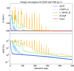
Figure 1: Comparison between the QITE algorithms and VQE of various optimizers (QOBYLA, L_BFGS_B and SLSQP) for $g=1$ (top panel) and $g=5$ (bottom panel) to reach the ground state energy of the NJL Hamiltonian. We use 4 qubits for the NJL model with $m=100$ MeV, $g=1$, $\mu=100$ MeV and $\mu_{5}=10$ MeV. For the VQE algorithm, the $x$-axis represents the number of optimization steps while for the QITE algorithms, the $x$-axis is the number of thermal evolution steps $x=\beta/\Delta\beta$ ($\Delta\beta=0.001$). We chose three optimizers provided by QISKIT and set the maximum optimization steps as 500 for all optimizers.

Besides calculating the ground state energy, another powerful application of the QITE algorithm is to simulating the temperature dependence of a thermal process. In this work, we will use the QITE algorithm introduced above to generate the thermal state $|\Psi(\beta/2)\rangle$, then apply the following relation to obtain the thermal average of an observable $\hat{O}$,

$$\langle\hat{O}\rangle_{\beta}=\frac{{\rm Tr}(e^{-\beta\hat{H}}\hat{O})}{{\rm Tr}(e^{-\beta\hat{H}})}=\frac{\sum_{i\in\mathcal{S}}\left<i\right|e^{-\beta\hat{H}/2}\hat{O}e^{-\beta\hat{H}/2}\left|i\right>}{\sum_{i\in\mathcal{S}}\left<i\right|e^{-\beta\hat{H}}\left|i\right>}\,.$$ (35)

Here $\mathcal{S}$ is a complete set as the basis of the ground state Motta et al. (2020). Specifically, we will choose $\hat{O}=\bar{\psi}\psi$ and $\hat{O}=\bar{\psi}\gamma_{0}\gamma_{5}\psi$ for calculating the thermal average of chiral condensate $\langle\bar{\psi}\psi\rangle$ and chirality charge density $n_{5}=\langle\bar{\psi}\gamma_{0}\gamma_{5}\psi\rangle$.

III Analytical calculation

In this section, before reaching out to quantum simulations, we first provide the analytical calculations for the chiral condensate and chirality charge density at finite temperature $T$, baryochemical potential $\mu$ and chiral chemical potential $\mu_{5}$ using the Lagrangian provided in Eq. (5) by minimizing the thermodynamic (Landau) potential.

III.1 The Landau potential and chiral condensate

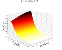
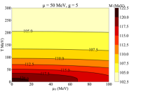
Figure 2: The effective mass $M$ as a function of the chiral chemical potential $\mu_{5}$ and temperature $T$ at $g=5$, chemical potential $\mu=50$ MeV. Upper: 3D Surface Plot. Lower: Contour Plot.

We first provide theoretical calculations for the vacuum chiral condensate $\langle\bar{\psi}\psi\rangle$ at various temperatures $T$, chemical potentials $\mu$ and $\mu_{5}$ under the Hamiltonian $\mathcal{H}$ as defined in Eq. (II.1). The chiral condensate $\langle\bar{\psi}\psi\rangle$, known to be an order parameter Gross et al. (1981); Nambu and Jona-Lasinio (1961c); McLerran and Svetitsky (1981); Polyakov (1978); Fang et al. (2018) for the chiral phase transition in the chiral limit ($m\sim 0$), has been studied in the mean field approximation. That is to say, as introduced in Gross and Neveu (1974); Walecka (1974), one writes $\bar{\psi}\psi=\langle\bar{\psi}\psi\rangle+\sigma$ with a constant term $\langle\bar{\psi}\psi\rangle$ and a small real scalar field $\sigma$, corresponding to fluctuations about the vacuum value, and then drop terms that are $\mathcal{O}(\sigma^{2})$. Then the four-fermion contact interaction $g(\bar{\psi}\psi)^{2}$ can be written as

$$g(\bar{\psi}\psi)^{2}= g\left(\langle\bar{\psi}\psi\rangle+\sigma\right)^{2}$$ (36)

$$= 2g\bar{\psi}\psi\langle\bar{\psi}\psi\rangle-g\langle\bar{\psi}\psi\rangle^{2}+\mathcal{O}(\sigma^{2}).$$

Furthermore, by defining the effective mass $M(\mu,\mu_{5},T)$ by

$$M(\mu,\mu_{5},T)=m-2g\langle\bar{\psi}\psi\rangle(\mu,\mu_{5},T),$$ (37)

the Lagrangian is given by $\mathcal{L}=\mathcal{L}_{\mathrm{eff}}+\mathcal{O}(\sigma^{2})$, where

$$\mathcal{L}_{\mathrm{eff}}= \bar{\psi}(i\not{\partial}-M+\mu\gamma_{0}+\mu_{5}\gamma_{0}\gamma_{5})\psi-\frac{(M-m)^{2}}{4g}$$

$$= \mathcal{L}_{\mathrm{Dirac}}-\mathcal{V}\,,$$ (38)

where the potential $\mathcal{V}$ is related to the chiral condensate as well as the effective mass

$$\mathcal{V}=g\langle\bar{\psi}\psi\rangle^{2}=(M-m)^{2}/4g.$$ (39)

Following Kapusta and Gale (2006); Buballa (2005), the Grand Canonical Potential $\Omega_{\mathrm{Dirac}}$ of $\mathcal{L}_{\mathrm{Dirac}}$ with mass $M$ is given in the following form

$$\Omega_{\mathrm{Dirac}}(\mu,\mu_{5},T;M)=-\frac{2}{\pi}\sum_{s=\pm 1}\int_{0}^{\infty}\bigg{[}T\ln(1+e^{-\beta(\omega_{k,s}+\mu)})$$

$$+T\ln(1+e^{-\beta(\omega_{k,s}-\mu)})+\omega_{k,s}\bigg{]}dk\,,$$ (40)

where the energy spectrum of the free fermions $\omega_{k,s}=\sqrt{(k+s\mu_{5})^{2}+M^{2}}$ with $s=\pm 1$. Then, by adding the potential $\mathcal{V}=(M-m)^{2}/4g$, we obtain the grand canonical potential for the NJL model as follows

$$\Omega(\mu,\mu_{5},T;M)=\mathcal{V}-\frac{2}{\pi}\sum_{s}\int_{0}^{\infty}\bigg{[}T\ln(1+e^{-\beta(\omega_{k,s}+\mu)})$$

$$+T\ln(1+e^{-\beta(\omega_{k,s}-\mu)})+\omega_{k,s}\bigg{]}dk\,.$$ (41)

Due to the divergent behavior of this quantity, one has to regularize it. In this work, for comparison with numerical results with the lattice spacing $a$, the natural momentum cutoff is $\Lambda=\pi/a$. With this hard momentum cutoff imposed for the integral shown in Eq. (III.1), one is able to determine the effective mass $M$ at fixed values of $\mu,~{}\mu_{5}$ and $T$ numerically by minimizing $\Omega(\mu,\mu_{5},T;M)$ in regard to $M$, namely solving the gap equation,

$$\frac{\partial\Omega(\mu,\mu_{5},T;M)}{\partial M}=0\,.$$ (42)

Then the chiral condensate is given by $\langle\bar{\psi}\psi\rangle=(m-M)/2g$ following Eq. (37).

As an example, in Fig. 2, we present the effective mass $M$ plot as a function of temperature $T$ and chiral chemical potential $\mu_{5}$ with bare mass $m=100$ MeV, coupling constant $g=5$, lattice spacing $a=1$ MeV^-1 and chemical potential $\mu=50$ MeV. As expected, at high $\mu_{5}$ or $T$, one has $M\rightarrow m$, corresponding to a restoration of chiral symmetry. Conversely, at low $(\mu_{5}^{2}+T^{2})$, one finds a dynamically generated mass of around $\Delta m\equiv M-m\sim 20$ MeV. Therefore, a free field theory is expected at asymptotically high temperatures/chemical potentials Gross and Neveu (1974).

III.2 The chirality charge density

In a magnetic field, under the imbalance of right/left-handed chirality, a finite induced current is produced along the magnetic field. Specifically, when the number of right-handed quarks, $N_{R}$ is unequal to that of the left-handed quarks $N_{L}$, positive charge is separated from negative charge along the magnetic field, which is the so-called “Chiral Magnetic Effect” Kharzeev and Zhitnitsky (2007); Kharzeev et al. (2008); Fukushima et al. (2008). The axial anomaly and topological objects in QCD are the fundamental physics of the CME. Unbalanced left- and right-handed quarks can produce observable effects that can be used to investigate topological $\mathcal{P}$- and $\mathcal{CP}$-odd excitations Witten (1979); Veneziano (1979); Schäfer and Shuryak (1998); Vicari and Panagopoulos (2009).

In Eq. (5), we have introduced an additional term with the chiral chemical potential $\mu_{5}$ coupled with the chirality charge density operator $n_{5}=\bar{\psi}\gamma_{0}\gamma_{5}\psi$, which has been known as a distinctive characteristic in hot and dense QCD matter and is not conserved as a consequence of the chiral anomaly. In the presence of a chiral chemical potential $\mu_{5}$, a manifestation of the chiral imbalance, the non-vanishing finite chirality charge density $n_{5}$ is required for the CME effect and recognized as a unique property of hot and dense QCD matter. Despite the fact that the chiral chemical potential $\mu_{5}$ is introduced for studying topological charge fluctuations, it is considered as a time-independent quantity that represents the chiral imbalance. And the chirality charge density $n_{5}=\langle\bar{\psi}\gamma_{0}\gamma_{5}\psi\rangle$ is a constant in the coordinates like the chiral condensate $\langle\bar{\psi}\psi\rangle$ .

When describing the induced electric current density as a function of the chirality density, the relationship between $n_{5}$ and $\mu_{5}$ is important and the chirality charge density $n_{5}$ can be calculated by Fukushima et al. (2010)

$$n_{5}= -\frac{\partial\Omega(\mu,\mu_{5},T;M)}{\partial\mu_{5}}\,,$$ (43)

where the grand potential $\Omega(\mu,\mu_{5},T;M)$ is given in Eq. (III.1). In the next section, we will present the analytical calculations of $n_{5}$ in comparison with QITE and exact diagonalization results.

IV Results

In this subsection, we study the finite temperature behaviors of the chiral condensate $\langle\bar{\psi}\psi\rangle$ and chirality charge density $n_{5}=\langle\bar{\psi}\gamma_{0}\gamma_{5}\psi\rangle$ in the $(1+1)$-dimensional NJL model given in Eq. (13). As emphasized in previous sections, we apply a quantum algorithm to simulate the thermal behaviours of physical observables. To demonstrate the reliability of our simulations, we will provide all the result from three different approaches:

1. QITE simulations of the thermal observable;

2. Exact diagonalizations from the discretization of the NJL Hamiltonian;

3. Analytical calculations given by solving the gap equation numerically.

For the consistency among the three procedures, we have chosen the same bare mass $m=100$ MeV and lattice spacing $a=1$ MeV^-1. The coupling constant $g$ at $g=1$ and $g=5$ are applied for testing the effects of the four-fermion interaction term in the Lagrangian.

To apply the quantum circuits, many quantum simulation packages have been developed and give similar results for quantum simulations. These quantum simulators, such as PYQUILL Smith et al. (2016) (Rigetti), TEQUILA Kottmann et al. (2021), Q# qsh (Microsoft), QISKIT Aleksandrowicz et al. (2019) (IBM), QFORTE Stair and Evangelista (2021), XACC McCaskey et al. (2020), FQE Rubin et al. (2021) CIRQ Developers (2021), are PYTHON software libraries and the outputs are the expected outputs of an ideal quantum computer. One can find a list of general quantum simulation packages in Bharti et al. (2022) and some implementations of the quantum algorithms are listed in Anand et al. (2021). To execute the QITE algorithm, we construct a quantum circuit using the open-source software package QFORTE Stair and Evangelista (2021), where many useful quantum algorithms have been implemented.

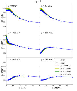
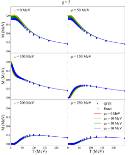
Figure 3: Chiral Condensate $\langle\bar{\psi}\psi\rangle$ as a function of temperature $T$ MeV at coupling constant $g=1$ (top panel) and $g=5$ (bottom panel) with a fixed chemical potential $\mu$ in each panel. Filled diamond points are given by QITE algorithm, hollow circle points are from exact diagonalization and solid curves are calculated analytically.

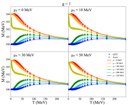
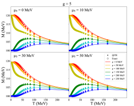
Figure 4: Chiral Condensate $\langle\bar{\psi}\psi\rangle$ as a function of temperature $T$ MeV at coupling constant $g=1$ (top panel) and $g=5$ (bottom panel) at a fixed chiral chemical potential $\mu_{5}$ in each panel.

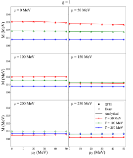
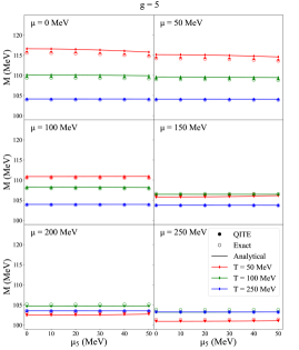
Figure 5: Chiral Condensate $\langle\bar{\psi}\psi\rangle$ as a function of $\mu_{5}$ at coupling constant $g=1$ (top panel) and $g=5$ (bottom panel).

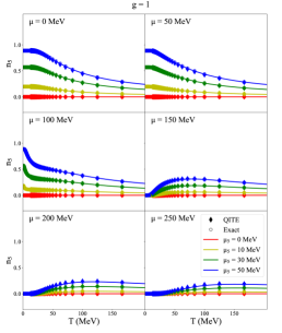
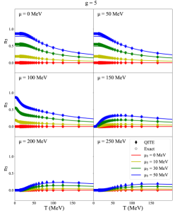
Figure 6: Chirality charge density $n_{5}$ as a function of temperature $T$ at $g=1$ (top panel) and $g=5$ (bottom panel) at a fixed chemical potential $\mu=0,50,100,\cdots,250$ MeV in each panel.

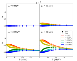
Figure 7: Chirality charge density $n_{5}$ as a function of temperature at $g=1$ (top panel) and $g=5$ (bottom panel) with a fixed chiral chemical potential $\mu_{5}$ in each panel.

IV.1 Chiral condensate

To study the effects of the chiral imbalance on the the chiral condensate at finite temperatures and chemical potentials, we present plots of the effective mass $M$ at various chemical potentials $\mu$, $\mu_{5}$ and temperatures $T$ in Figs. 3, 4 and 5, respectively. In Fig. 3, we compare the temperature dependence of the effective mass $M$ at $g=1$ and $g=5$ as a function of temperature $T$ at chiral chemical potential $\mu_{5}=0,\ 10,\ 30$ and $50$ MeV with a fixed baryochemical potentials $\mu\in\{0,\ 50,\cdots,250\}$ MeV in each panel, where filled diamond points are given by the QITE algorithm, hollow circle points are from exact diagonalization and solid curve results are calculated analytically. Between $\mu=100$ MeV and $\mu=150$ MeV panels, the pattern of the effective mass changed from decreasing ($\mu\leq 100$ MeV) to increasing with temperature ($\mu\geq 150$ MeV). Also for $\mu\leq 100$ MeV panels, the effective mass $M$ at smaller $\mu_{5}$ is larger, while for $\mu\geq 150$ MeV panels, the effective mass $M$ at smaller $\mu_{5}$ is smaller.

In Fig. 4, we fix the value of chiral chemical potentials $\mu_{5}$ in each panel and plot the $M\mathrm{-}T$ curves at various baryochemical potentials $\mu=0,\ 50,\cdots,250$ MeV at $g=1$ and $g=5$. A non-trivial phase transition at $100<\mu<150$ MeV is observed in all the panels and this has also been pointed out when interpreting Fig. 4. The patterns look similar at various $\mu_{5}$ and we find that at smaller $\mu_{5}$, the effective mass $M$ changes more rapidly as a function of $T$.

To better illustrate the effects of $\mu_{5}$, we present the effective mass $M$ as a function of chiral chemical potentials $\mu_{5}$ and show the results at several temperatures and baryochemical potentials in Fig. 5 for $g=1$ and $g=5$. The effective mass changes slightly as the chiral chemical potential increases, indicating that the chiral chemical potential plays a lesser role in chiral symmetry breaking than the temperature and chemical potential, at least in this model. At $\mu\leq 100$ MeV, $M$ is lower for higher temperature, which is expected by the asymptotic freedom. While as $\mu$ increases, the effective mass $M$ becomes smaller at lower temperatures.

IV.2 Chirality charge density

In this subsection, we present the results for the chirality charge density $n_{5}$ using the QITE algorithm in comparison with analytical calculations as introduced in Sec. III.2 and exact diagonalization.

In Fig. 6, we plot the chirality charge density as a function of temperature $T$ at coupling constant $g=1$ and $g=5$. We use different colors to distinguish various chiral chemical potentials $\mu_{5}=0,\ 10,\ 30$ and $50$ MeV and in each panel, the chemical potential $\mu$ is fixed at $0,\ 50,\ 100,\cdots$ or $250$ MeV. At $\mu_{5}=0$ MeV, one obtains $n_{5}=0$ since there is no other mechanism for generating a nonzero $\mathcal{N}_{5}=\bar{\psi}\gamma_{0}\gamma_{5}\psi=\psi^{\dagger}_{R}\psi_{R}-\psi^{\dagger}_{L}\psi_{L}$. As a result, only when $\mu_{5}\neq 0$, there exists non-zero $n_{5}=\langle\mathcal{N}_{5}\rangle$.

Similar to what was observed in the effective mass plots in Fig. 3, a non-trivial phase transition is observed between $\mu=100$ MeV and $\mu=150$ MeV. For $\mu\leq 100$ MeV, the chirality charge density decreases as temperature rises, while for $\mu\geq 150$ MeV, the chirality charge density first increases then drops and converges to $0$ with the increasing of temperature.

In Fig. 7, we plot the chirality charge density $n_{5}$ as a function of temperature $T$ at coupling constants $g=1$ and $g=5$. We use different colors to distinguish various chemical potentials $\mu\in\{0,\ 50,\cdots,250\}$ MeV and in each panel, the chemical potential $\mu_{5}$ is fixed at $0,\ 10,\ 30$ or $50$ MeV. At $\mu_{5}=0$ MeV, the chirality charge density is $0$ at all temperatures and chemical potentials, as expected from the previous figure. At non-zero $\mu_{5}$ values, the phase transition between $\mu=100$ MeV and $\mu=150$ MeV can also be observed: for $\mu\leq 100$ MeV, the chirality charge density begins at some non-zero value at $T=0$ MeV and decreases with temperature, while for curves $\mu\geq 150$ MeV, the chirality charge density begins at $0$ at $T=0$ MeV and first increases before decreasing and converging to 0 with increasing temperature. At greater values of $\mu_{5}$, curves with $\mu\leq 100$ MeV begin at higher chirality charge densities.

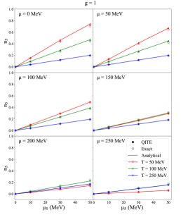
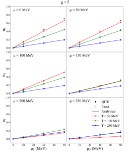
Figure 8: Chirality charge density $n_{5}$ as a function of chiral chemical potential $\mu_{5}$ at $g=1$ (top panel) and $g=5$ (bottom panel) with a fixed temperature $T$ in each panel.

In Fig. 8, we plot the chirality charge density $n_{5}$ as a function of chiral chemical potential $\mu_{5}$ at coupling constants $g=1$ and $g=5$. Colors are used to distinguish between different various temperatures $T=50,\ 100,\$ or $200$ MeV, and the chemical potential is fixed at $\mu=0,\ 50,\cdots,250$ MeV in each panel. At all chemical potentials $\mu$ and temperatures $T$, we see that (approximately) $n_{5}\propto\mu_{5}$: the chirality charge density $n_{5}$ begins at $0$ MeV at $\mu_{5}=0$ MeV, and increases linearly with $\mu_{5}$. The chiral chemical potential $\mu_{5}$, at least in this model, is thus a direct measure of chiral imbalance in the plasma. Higher chemical potentials $\mu$ result in a slower increase of $n_{5}$ with $\mu_{5}$. Once again, a phase transition can be observed between $\mu\leq 100$ MeV and $\mu\geq 150$ MeV. For $\mu\leq 100$ MeV, at each $\mu_{5}$, $n_{5}$ decreases with increasing temperature. For $\mu\geq 150$ MeV, $n_{5}$ first increases with temperature from $T=50$ MeV to $T=100$ MeV, but then decreases from $T=100$ MeV to $T=200$ MeV.

V Conclusion

In conclusion, using the QITE algorithm, we performed a quantum simulation for the chiral phase transition of the 1+1 dimensional NJL model at finite temperature, baryochemical potential and chiral chemical potential. Specifically, we use a 4-qubit quantum circuit to simulate the NJL Hamiltonian and find that the results among the digital quantum simulation, exact diagonalization, and analytical analysis are all consistent, implying that quantum computing will be a promising tool in simulating finite-temperature behaviors in the future for QCD.

The quantum simulations’ efficacy has been shown to be insensitive to the chemical potentials $\mu$ and $\mu_{5}$ (and possibly other external parameters), which opens up new possibilities for studying finite density effects in QCD and other field theories. Owing to technological constraints (nonperturbative dynamics, Monte Carlo failure due to the sign problem, etc.) restricting the use of typical computing methods, this element of quark physics remains substantially unexplored in comparison to other fields. With the development of scalable quantum computing technologies on the horizon, Lattice QCD calculations on quantum computers are becoming not only conceivable, but also practical.

This research, together with prior research, shows that NISQ quantum computers may produce consistent and correct answers to physical issues that cannot be solved efficiently or effectively using classical computing algorithms, reflecting bright prospects for future applications of quantum computing to non-perturbative QCD in the NISQ era and beyond.

References

- Fukushima et al. (2010) K. Fukushima, M. Ruggieri, and R. Gatto, Phys. Rev. D 81, 114031 (2010), arXiv:1003.0047 [hep-ph] .
- Buballa (2005) M. Buballa, Phys. Rept. 407, 205 (2005), arXiv:hep-ph/0402234 .
- McLerran and Pisarski (2007) L. McLerran and R. D. Pisarski, Nucl. Phys. A 796, 83 (2007), arXiv:0706.2191 [hep-ph] .
- McLerran et al. (2009) L. McLerran, K. Redlich, and C. Sasaki, Nucl. Phys. A 824, 86 (2009), arXiv:0812.3585 [hep-ph] .
- Menezes et al. (2009a) D. P. Menezes, M. B. Pinto, S. S. Avancini, A. P. Martínez, and C. Providência, Phys. Rev. C 79, 035807 (2009a).
- Orsaria et al. (2014) M. Orsaria, H. Rodrigues, F. Weber, and G. A. Contrera, Phys. Rev. C 89, 015806 (2014), arXiv:1308.1657 [nucl-th] .
- Ruggieri and Peng (2016) M. Ruggieri and G. X. Peng, Phys. Rev. D 93, 094021 (2016), arXiv:1602.08994 [hep-ph] .
- Jiménez (2021) J. C. Jiménez, Interacting quark matter effects on the structure of compact stars, Other thesis (2021), arXiv:2104.03551 [hep-ph] .
- Gyulassy and McLerran (2005) M. Gyulassy and L. McLerran, Nucl. Phys. A 750, 30 (2005), arXiv:nucl-th/0405013 .
- Soloveva et al. (2021) O. Soloveva, D. Fuseau, J. Aichelin, and E. Bratkovskaya, Phys. Rev. C 103, 054901 (2021), arXiv:2011.03505 [nucl-th] .
- Fukushima and Hatsuda (2011) K. Fukushima and T. Hatsuda, Rept. Prog. Phys. 74, 014001 (2011), arXiv:1005.4814 [hep-ph] .
- Choudhury et al. (2022) S. Choudhury et al., Chin. Phys. C 46, 014101 (2022), arXiv:2105.06044 [nucl-ex] .
- Feng et al. (2022) Y. Feng, J. Zhao, H. Li, H.-j. Xu, and F. Wang, Phys. Rev. C 105, 024913 (2022), arXiv:2106.15595 [nucl-ex] .
- Abdallah et al. (2022a) M. Abdallah et al. (STAR), Phys. Rev. C 105, 014901 (2022a), arXiv:2109.00131 [nucl-ex] .
- Milton et al. (2021) R. Milton, G. Wang, M. Sergeeva, S. Shi, J. Liao, and H. Z. Huang, Phys. Rev. C 104, 064906 (2021), arXiv:2110.01435 [nucl-th] .
- Kharzeev et al. (2022) D. E. Kharzeev, J. Liao, and S. Shi, (2022), arXiv:2205.00120 [nucl-th] .
- Kharzeev (2022) D. E. Kharzeev (2022) arXiv:2204.10903 [hep-ph] .
- Adhikari (2022) P. Adhikari, Nucl. Phys. B 974, 115627 (2022), arXiv:2111.06196 [hep-ph] .
- Tawfik and Diab (2021) A. N. Tawfik and A. M. Diab, Eur. Phys. J. A 57, 200 (2021), arXiv:2106.04576 [hep-ph] .
- Cao (2021) G. Cao, Eur. Phys. J. A 57, 264 (2021), arXiv:2103.00456 [hep-ph] .
- Moreira et al. (2021) J. a. Moreira, P. Costa, and T. E. Restrepo, Eur. Phys. J. A 57, 123 (2021), arXiv:2101.12004 [hep-ph] .
- Ding et al. (2021) H. T. Ding, S. T. Li, A. Tomiya, X. D. Wang, and Y. Zhang, Phys. Rev. D 104, 014505 (2021), arXiv:2008.00493 [hep-lat] .
- Zhao and Wang (2019) J. Zhao and F. Wang, Prog. Part. Nucl. Phys. 107, 200 (2019), arXiv:1906.11413 [nucl-ex] .
- Tawfik et al. (2019) A. N. Tawfik, A. M. Diab, and M. T. Hussein, Chin. Phys. C 43, 034103 (2019), arXiv:1901.03293 [hep-ph] .
- Gusynin et al. (1999) V. P. Gusynin, V. A. Miransky, and I. A. Shovkovy, Nucl. Phys. B 563, 361 (1999), arXiv:hep-ph/9908320 .
- Klimenko (1991) K. G. Klimenko, Teor. Mat. Fiz. 89, 211 (1991).
- Klevansky and Lemmer (1989) S. P. Klevansky and R. H. Lemmer, Phys. Rev. D 39, 3478 (1989).
- Kharzeev and Zhitnitsky (2007) D. Kharzeev and A. Zhitnitsky, Nucl. Phys. A 797, 67 (2007), arXiv:0706.1026 [hep-ph] .
- Kharzeev et al. (2008) D. E. Kharzeev, L. D. McLerran, and H. J. Warringa, Nucl. Phys. A 803, 227 (2008), arXiv:0711.0950 [hep-ph] .
- Fukushima et al. (2008) K. Fukushima, D. E. Kharzeev, and H. J. Warringa, Phys. Rev. D 78, 074033 (2008), arXiv:0808.3382 [hep-ph] .
- Diakonov (2003) D. Diakonov, Prog. Part. Nucl. Phys. 51, 173 (2003), arXiv:hep-ph/0212026 .
- Schäfer and Shuryak (1996) T. Schäfer and E. V. Shuryak, Phys. Rev. D 53, 6522 (1996), arXiv:hep-ph/9509337 .
- Arnold and McLerran (1988) P. B. Arnold and L. D. McLerran, Phys. Rev. D 37, 1020 (1988).
- Fukugita and Yanagida (1990) M. Fukugita and T. Yanagida, Phys. Rev. D 42, 1285 (1990).
- McLerran et al. (1991) L. D. McLerran, E. Mottola, and M. E. Shaposhnikov, Phys. Rev. D 43, 2027 (1991).
- Witten (1979) E. Witten, Nucl. Phys. B 156, 269 (1979).
- Veneziano (1979) G. Veneziano, Nucl. Phys. B 159, 213 (1979).
- Schäfer and Shuryak (1998) T. Schäfer and E. V. Shuryak, Rev. Mod. Phys. 70, 323 (1998), arXiv:hep-ph/9610451 .
- Vicari and Panagopoulos (2009) E. Vicari and H. Panagopoulos, Phys. Rept. 470, 93 (2009), arXiv:0803.1593 [hep-th] .
- Kharzeev et al. (2016) D. E. Kharzeev, J. Liao, S. A. Voloshin, and G. Wang, Prog. Part. Nucl. Phys. 88, 1 (2016), arXiv:1511.04050 [hep-ph] .
- Bzdak et al. (2020) A. Bzdak, S. Esumi, V. Koch, J. Liao, M. Stephanov, and N. Xu, Phys. Rept. 853, 1 (2020), arXiv:1906.00936 [nucl-th] .
- Chen and Feng (2020) B.-X. Chen and S.-Q. Feng, Chin. Phys. C 44, 024104 (2020), arXiv:1909.10836 [hep-ph] .
- Voloshin (2004) S. A. Voloshin, Phys. Rev. C 70, 057901 (2004), arXiv:hep-ph/0406311 .
- Abelev et al. (2010) B. I. Abelev et al. (STAR), Phys. Rev. C 81, 054908 (2010), arXiv:0909.1717 [nucl-ex] .
- Abelev et al. (2009) B. I. Abelev et al. (STAR), Phys. Rev. Lett. 103, 251601 (2009), arXiv:0909.1739 [nucl-ex] .
- Hu (2022) Y. Hu (STAR), EPJ Web Conf. 259, 13013 (2022), arXiv:2110.15937 [nucl-ex] .
- Abdallah et al. (2022b) M. Abdallah et al. (STAR), Phys. Rev. Lett. 128, 092301 (2022b), arXiv:2106.09243 [nucl-ex] .
- Zhao (2021) J. Zhao (STAR), Nucl. Phys. A 1005, 121766 (2021), arXiv:2002.09410 [nucl-ex] .
- Abelev et al. (2013) B. Abelev et al. (ALICE), Phys. Rev. Lett. 110, 012301 (2013), arXiv:1207.0900 [nucl-ex] .
- Adam et al. (2016) J. Adam et al. (ALICE), Phys. Rev. C 93, 044903 (2016), arXiv:1512.05739 [nucl-ex] .
- Parmar (2018) S. Parmar (ALICE), Springer Proc. Phys. 203, 785 (2018), arXiv:1703.09496 [hep-ex] .
- Acharya et al. (2018) S. Acharya et al. (ALICE), Phys. Lett. B 777, 151 (2018), arXiv:1709.04723 [nucl-ex] .
- Acharya et al. (2020) S. Acharya et al. (ALICE), JHEP 09, 160 (2020), arXiv:2005.14640 [nucl-ex] .
- Sirunyan et al. (2018) A. M. Sirunyan et al. (CMS), Phys. Rev. C 97, 044912 (2018), arXiv:1708.01602 [nucl-ex] .
- Khachatryan et al. (2017) V. Khachatryan et al. (CMS), Phys. Rev. Lett. 118, 122301 (2017), arXiv:1610.00263 [nucl-ex] .
- Kharzeev and Kikuchi (2020) D. E. Kharzeev and Y. Kikuchi, Phys. Rev. Res. 2, 023342 (2020), arXiv:2001.00698 [hep-ph] .
- Ruggieri et al. (2016) M. Ruggieri, G. X. Peng, and M. Chernodub, Phys. Rev. D 94, 054011 (2016), arXiv:1606.03287 [hep-ph] .
- Ruggieri et al. (2020) M. Ruggieri, M. N. Chernodub, and Z.-Y. Lu, Phys. Rev. D 102, 014031 (2020), arXiv:2004.09393 [hep-ph] .
- Nambu and Jona-Lasinio (1961a) Y. Nambu and G. Jona-Lasinio, Phys. Rev. 122, 345 (1961a).
- Nambu and Jona-Lasinio (1961b) Y. Nambu and G. Jona-Lasinio, Phys. Rev. 124, 246 (1961b).
- Fukushima (2008) K. Fukushima, Phys. Rev. D 77, 114028 (2008).
- Costa et al. (2007) P. Costa, C. de Sousa, M. Ruivo, and Y. Kalinovsky, Physics Letters B 647, 431 (2007).
- Lu et al. (2015) Y. Lu, Y.-L. Du, Z.-F. Cui, and H.-S. Zong, The European Physical Journal C 75, 495 (2015).
- Du et al. (2015) Y.-L. Du, Y. Lu, S.-S. Xu, Z.-F. Cui, C. Shi, and H.-S. Zong, International Journal of Modern Physics A 30, 1550199 (2015), https://doi.org/10.1142/S0217751X15501997 .
- Cui et al. (2015) Z.-F. Cui, F.-Y. Hou, Y.-M. Shi, Y.-L. Wang, and H.-S. Zong, Annals of Physics 358, 172 (2015), school of Physics at Nanjing University.
- Du et al. (2013) Y.-l. Du, Z.-f. Cui, Y.-h. Xia, and H.-s. Zong, Phys. Rev. D 88, 114019 (2013).
- Shi et al. (2015) S. Shi, Y.-C. Yang, Y.-H. Xia, Z.-F. Cui, X.-J. Liu, and H.-S. Zong, Phys. Rev. D 91, 036006 (2015).
- Menezes et al. (2009b) D. P. Menezes, M. B. Pinto, S. S. Avancini, and C. Providência, Phys. Rev. C 80, 065805 (2009b).
- Ghosh et al. (2007) S. Ghosh, S. Mandal, and S. Chakrabarty, Phys. Rev. C 75, 015805 (2007).
- Bali et al. (2012) G. S. Bali, F. Bruckmann, G. Endrődi, Z. Fodor, S. D. Katz, and A. Schäfer, Phys. Rev. D 86, 071502 (2012).
- Yamamoto (2011) A. Yamamoto, Phys. Rev. Lett. 107, 031601 (2011), arXiv:1105.0385 [hep-lat] .
- Braguta et al. (2016) V. V. Braguta, E. M. Ilgenfritz, A. Y. Kotov, B. Petersson, and S. A. Skinderev, Phys. Rev. D 93, 034509 (2016), arXiv:1512.05873 [hep-lat] .
- Braguta et al. (2015) V. V. Braguta, V. A. Goy, E. M. Ilgenfritz, A. Y. Kotov, A. V. Molochkov, M. Muller-Preussker, and B. Petersson, JHEP 06, 094 (2015), arXiv:1503.06670 [hep-lat] .
- Alexandru et al. (2016) A. Alexandru, G. Basar, and P. Bedaque, Phys. Rev. D 93, 014504 (2016), arXiv:1510.03258 [hep-lat] .
- Scorzato (2016) L. Scorzato, PoS LATTICE2015, 016 (2016), arXiv:1512.08039 [hep-lat] .
- Braguta and Kotov (2016) V. V. Braguta and A. Y. Kotov, Phys. Rev. D 93, 105025 (2016), arXiv:1601.04957 [hep-th] .
- Kapusta and Gale (2006) J. I. Kapusta and C. Gale, Finite-Temperature Field Theory: Principles and Applications, 2nd ed., Cambridge Monographs on Mathematical Physics (Cambridge University Press, 2006).
- Feynman (1982) R. P. Feynman, International Journal of Theoretical Physics 21, 467 (1982).
- Bauer et al. (2020) B. Bauer, S. Bravyi, M. Motta, and G. K.-L. Chan, Chemical Reviews 120, 12685–12717 (2020).
- Terhal and DiVincenzo (2000a) B. M. Terhal and D. P. DiVincenzo, Phys. Rev. A 61, 022301 (2000a).
- Poulin and Wocjan (2009) D. Poulin and P. Wocjan, Phys. Rev. Lett. 103, 220502 (2009).
- Riera et al. (2012) A. Riera, C. Gogolin, and J. Eisert, Phys. Rev. Lett. 108, 080402 (2012).
- Temme et al. (2011a) K. Temme, T. J. Osborne, K. G. Vollbrecht, D. Poulin, and F. Verstraete, Nature 471, 87 (2011a).
- Yung and Aspuru-Guzik (2012) M.-H. Yung and A. Aspuru-Guzik, Proceedings of the National Academy of Sciences 109, 754 (2012).
- Li et al. (2021) T. Li, X. Guo, W. K. Lai, X. Liu, E. Wang, H. Xing, D.-B. Zhang, and S.-L. Zhu, (2021), arXiv:2106.03865 [hep-ph] .
- Zhang et al. (2021) D.-B. Zhang, H. Xing, H. Yan, E. Wang, and S.-L. Zhu, Chin. Phys. B 30, 020306 (2021), arXiv:2011.01431 [quant-ph] .
- Tomiya (2022) A. Tomiya, (2022), arXiv:2205.08860 [hep-lat] .
- Xie et al. (2022) X.-D. Xie, X. Guo, H. Xing, Z.-Y. Xue, D.-B. Zhang, and S.-L. Zhu (QuNu), Phys. Rev. D 106, 054509 (2022), arXiv:2205.12767 [quant-ph] .
- Davoudi et al. (2022) Z. Davoudi, N. Mueller, and C. Powers, (2022), arXiv:2208.13112 [hep-lat] .
- Arute et al. (2020) F. Arute et al., Science 369, 1084 (2020), arXiv:2004.04174 [quant-ph] .
- Ma et al. (2020) H. Ma, M. Govoni, and G. Galli, npj Computational Materials 6, 85 (2020).
- Kandala et al. (2019) A. Kandala, K. Temme, A. D. Córcoles, A. Mezzacapo, J. M. Chow, and J. M. Gambetta, Nature 567, 491 (2019).
- O’Malley et al. (2016) P. J. J. O’Malley, R. Babbush, I. D. Kivlichan, J. Romero, J. R. McClean, R. Barends, J. Kelly, P. Roushan, A. Tranter, N. Ding, B. Campbell, Y. Chen, Z. Chen, B. Chiaro, A. Dunsworth, A. G. Fowler, E. Jeffrey, E. Lucero, A. Megrant, J. Y. Mutus, M. Neeley, C. Neill, C. Quintana, D. Sank, A. Vainsencher, J. Wenner, T. C. White, P. V. Coveney, P. J. Love, H. Neven, A. Aspuru-Guzik, and J. M. Martinis, Phys. Rev. X 6, 031007 (2016).
- Kandala et al. (2017) A. Kandala, A. Mezzacapo, K. Temme, M. Takita, M. Brink, J. M. Chow, and J. M. Gambetta, Nature 549, 242 (2017).
- Peruzzo et al. (2014) A. Peruzzo, J. McClean, P. Shadbolt, M.-H. Yung, X.-Q. Zhou, P. J. Love, A. Aspuru-Guzik, and J. L. O’Brien, Nature Communications 5, 4213 (2014).
- Colless et al. (2018) J. I. Colless, V. V. Ramasesh, D. Dahlen, M. S. Blok, M. E. Kimchi-Schwartz, J. R. McClean, J. Carter, W. A. de Jong, and I. Siddiqi, Phys. Rev. X 8, 011021 (2018).
- Chiesa et al. (2019) A. Chiesa, F. Tacchino, M. Grossi, P. Santini, I. Tavernelli, D. Gerace, and S. Carretta, Nature Physics 15, 455 (2019).
- Smith et al. (2019) A. Smith, M. S. Kim, F. Pollmann, and J. Knolle, npj Quantum Information 5, 106 (2019).
- Zhang et al. (2017) J. Zhang, G. Pagano, P. W. Hess, A. Kyprianidis, P. Becker, H. Kaplan, A. V. Gorshkov, Z. X. Gong, and C. Monroe, Nature 551, 601 (2017).
- Islam et al. (2013) R. Islam, C. Senko, W. C. Campbell, S. Korenblit, J. Smith, A. Lee, E. E. Edwards, C.-C. J. Wang, J. K. Freericks, and C. Monroe, Science 340, 583 (2013).
- Francis et al. (2020) A. Francis, J. K. Freericks, and A. F. Kemper, Phys. Rev. B 101, 014411 (2020).
- Lloyd (1996) S. Lloyd, Science 273, 1073 (1996).
- De Jong et al. (2021) W. A. De Jong, M. Metcalf, J. Mulligan, M. Płoskoń, F. Ringer, and X. Yao, Phys. Rev. D 104, 051501 (2021), arXiv:2010.03571 [hep-ph] .
- de Jong et al. (2021) W. A. de Jong, K. Lee, J. Mulligan, M. Płoskoń, F. Ringer, and X. Yao, (2021), arXiv:2106.08394 [quant-ph] .
- Wallraff et al. (2004) A. Wallraff, D. I. Schuster, A. Blais, L. Frunzio, R.-S. Huang, J. Majer, S. Kumar, S. M. Girvin, and R. J. Schoelkopf, Nature 431, 162 (2004), bandiera_abtest: a Cg_type: Nature Research Journals Number: 7005 Primary_atype: Research Publisher: Nature Publishing Group.
- Majer et al. (2007) J. Majer, J. M. Chow, J. M. Gambetta, J. Koch, B. R. Johnson, J. A. Schreier, L. Frunzio, D. I. Schuster, A. A. Houck, A. Wallraff, A. Blais, M. H. Devoret, S. M. Girvin, and R. J. Schoelkopf, Nature 449, 443 (2007), bandiera_abtest: a Cg_type: Nature Research Journals Number: 7161 Primary_atype: Research Publisher: Nature Publishing Group.
- Jordan et al. (2012) S. P. Jordan, K. S. M. Lee, and J. Preskill, Science 336, 1130 (2012), arXiv: 1111.3633.
- Zohar et al. (2012) E. Zohar, J. I. Cirac, and B. Reznik, Physical Review Letters 109, 125302 (2012), publisher: American Physical Society.
- Zohar et al. (2013) E. Zohar, J. I. Cirac, and B. Reznik, Physical Review Letters 110, 125304 (2013), publisher: American Physical Society.
- Banerjee et al. (2013) D. Banerjee, M. Bögli, M. Dalmonte, E. Rico, P. Stebler, U.-J. Wiese, and P. Zoller, Physical Review Letters 110, 125303 (2013), publisher: American Physical Society.
- Banerjee et al. (2012) D. Banerjee, M. Dalmonte, M. Müller, E. Rico, P. Stebler, U.-J. Wiese, and P. Zoller, Physical Review Letters 109, 175302 (2012), arXiv: 1205.6366.
- Wiese (2013) U.-J. Wiese, Annalen der Physik 525, 777 (2013), _eprint: https://onlinelibrary.wiley.com/doi/pdf/10.1002/andp.201300104.
- Wiese (2014) U.-J. Wiese, Nuclear Physics A QUARK MATTER 2014, 931, 246 (2014).
- Jordan et al. (2014) S. P. Jordan, K. S. M. Lee, and J. Preskill, arXiv:1404.7115 [hep-th, physics:quant-ph] (2014), arXiv: 1404.7115.
- García-Álvarez et al. (2015) L. García-Álvarez, J. Casanova, A. Mezzacapo, I. L. Egusquiza, L. Lamata, G. Romero, and E. Solano, Physical Review Letters 114, 070502 (2015), publisher: American Physical Society.
- Marcos et al. (2014) D. Marcos, P. Widmer, E. Rico, M. Hafezi, P. Rabl, U. J. Wiese, and P. Zoller, Annals of Physics 351, 634 (2014).
- Bazavov et al. (2015) A. Bazavov, Y. Meurice, S.-W. Tsai, J. Unmuth-Yockey, and J. Zhang, Physical Review D 92, 076003 (2015), publisher: American Physical Society.
- Zohar et al. (2015) E. Zohar, J. I. Cirac, and B. Reznik, Reports on Progress in Physics 79, 014401 (2015), publisher: IOP Publishing.
- Mezzacapo et al. (2015) A. Mezzacapo, E. Rico, C. Sabín, I. L. Egusquiza, L. Lamata, and E. Solano, Physical Review Letters 115, 240502 (2015), publisher: American Physical Society.
- Dalmonte and Montangero (2016) M. Dalmonte and S. Montangero, Contemporary Physics 57, 388 (2016), arXiv: 1602.03776.
- Zohar et al. (2017) E. Zohar, A. Farace, B. Reznik, and J. I. Cirac, Physical Review A 95, 023604 (2017), arXiv: 1607.08121.
- Martinez et al. (2016) E. A. Martinez, C. A. Muschik, P. Schindler, D. Nigg, A. Erhard, M. Heyl, P. Hauke, M. Dalmonte, T. Monz, P. Zoller, and R. Blatt, Nature 534, 516 (2016), arXiv: 1605.04570.
- Bermudez et al. (2017) A. Bermudez, G. Aarts, and M. Müller, Physical Review X 7, 041012 (2017), publisher: American Physical Society.
- Gambetta et al. (2017) J. M. Gambetta, J. M. Chow, and M. Steffen, npj Quantum Information 3, 1 (2017), bandiera_abtest: a Cc_license_type: cc_by Cg_type: Nature Research Journals Number: 1 Primary_atype: Reviews Publisher: Nature Publishing Group Subject_term: Quantum information;Qubits Subject_term_id: quantum-information;qubits.
- Krinner et al. (2018) L. Krinner, M. Stewart, A. Pazmiño, J. Kwon, and D. Schneble, Nature 559, 589 (2018), bandiera_abtest: a Cg_type: Nature Research Journals Number: 7715 Primary_atype: Research Publisher: Nature Publishing Group Subject_term: Matter waves and particle beams;Quantum simulation;Single photons and quantum effects;Ultracold gases Subject_term_id: matter-waves-and-particle-beams;quantum-simulation;single-photons-and-quantum-effects;ultracold-gases.
- Macridin et al. (2018) A. Macridin, P. Spentzouris, J. Amundson, and R. Harnik, Physical Review Letters 121, 110504 (2018), publisher: American Physical Society.
- Zache et al. (2018) T. V. Zache, F. Hebenstreit, F. Jendrzejewski, M. K. Oberthaler, J. Berges, and P. Hauke, Quantum Science and Technology 3, 034010 (2018), publisher: IOP Publishing.
- Zhang et al. (2018) J. Zhang, J. Unmuth-Yockey, J. Zeiher, A. Bazavov, S.-W. Tsai, and Y. Meurice, Physical Review Letters 121, 223201 (2018), publisher: American Physical Society.
- Klco et al. (2018) N. Klco, E. F. Dumitrescu, A. J. McCaskey, T. D. Morris, R. C. Pooser, M. Sanz, E. Solano, P. Lougovski, and M. J. Savage, Physical Review A 98, 032331 (2018), arXiv: 1803.03326.
- Klco and Savage (2019) N. Klco and M. J. Savage, Physical Review A 99, 052335 (2019), arXiv: 1808.10378.
- Gustafson et al. (2019) E. Gustafson, Y. Meurice, and J. Unmuth-Yockey, Physical Review D 99, 094503 (2019), publisher: American Physical Society.
- NuQS Collaboration et al. (2019) NuQS Collaboration, A. Alexandru, P. F. Bedaque, H. Lamm, and S. Lawrence, Physical Review Letters 123, 090501 (2019), publisher: American Physical Society.
- Magnifico et al. (2020) G. Magnifico, M. Dalmonte, P. Facchi, S. Pascazio, F. V. Pepe, and E. Ercolessi, Quantum 4, 281 (2020), arXiv: 1909.04821.
- Jordan et al. (2019) S. P. Jordan, K. S. M. Lee, and J. Preskill, arXiv:1112.4833 [hep-th, physics:quant-ph] (2019), arXiv: 1112.4833.
- Lu et al. (2019) H.-H. Lu, N. Klco, J. M. Lukens, T. D. Morris, A. Bansal, A. Ekström, G. Hagen, T. Papenbrock, A. M. Weiner, M. J. Savage, and P. Lougovski, Physical Review A 100, 012320 (2019), arXiv: 1810.03959.
- Klco and Savage (2020) N. Klco and M. J. Savage, Physical Review A 102, 012612 (2020), arXiv: 1904.10440.
- Lamm and Lawrence (2018) H. Lamm and S. Lawrence, Physical Review Letters 121, 170501 (2018), arXiv: 1806.06649.
- Klco et al. (2020) N. Klco, J. R. Stryker, and M. J. Savage, Physical Review D 101, 074512 (2020), arXiv: 1908.06935.
- Alexandru et al. (2019) A. Alexandru, P. F. Bedaque, S. Harmalkar, H. Lamm, S. Lawrence, and N. C. Warrington, Physical Review D 100, 114501 (2019), arXiv: 1906.11213.
- Mueller et al. (2020) N. Mueller, A. Tarasov, and R. Venugopalan, Physical Review D 102, 016007 (2020), arXiv: 1908.07051.
- Lamm et al. (2020) H. Lamm, S. Lawrence, and Y. Yamauchi, Physical Review Research 2, 013272 (2020), arXiv: 1908.10439.
- Chakraborty et al. (2020) B. Chakraborty, M. Honda, T. Izubuchi, Y. Kikuchi, and A. Tomiya, arXiv:2001.00485 [cond-mat, physics:hep-lat, physics:hep-ph, physics:hep-th, physics:quant-ph] (2020), arXiv: 2001.00485.
- Bermudez et al. (2018) A. Bermudez, E. Tirrito, M. Rizzi, M. Lewenstein, and S. Hands, Annals Phys. 399, 149 (2018), arXiv:1807.03202 [cond-mat.quant-gas] .
- Ziegler et al. (2020) L. Ziegler, E. Tirrito, M. Lewenstein, S. Hands, and A. Bermudez, (2020), arXiv:2011.08744 [cond-mat.quant-gas] .
- Ziegler et al. (2021) L. Ziegler, E. Tirrito, M. Lewenstein, S. Hands, and A. Bermudez, (2021), arXiv:2111.04485 [cond-mat.quant-gas] .
- Sun et al. (2021) S.-N. Sun, M. Motta, R. N. Tazhigulov, A. T. Tan, G. K.-L. Chan, and A. J. Minnich, PRX Quantum 2, 010317 (2021).
- Ville et al. (2021) J.-L. Ville et al., (2021), arXiv:2104.08785 [quant-ph] .
- Czajka et al. (2022) A. M. Czajka, Z.-B. Kang, H. Ma, and F. Zhao, JHEP 08, 209 (2022), arXiv:2112.03944 [hep-ph] .
- Gross and Neveu (1974) D. J. Gross and A. Neveu, Phys. Rev. D 10, 3235 (1974).
- Borsanyi et al. (2010) S. Borsanyi, G. Endrodi, Z. Fodor, A. Jakovac, S. D. Katz, S. Krieg, C. Ratti, and K. K. Szabo, JHEP 11, 077 (2010), arXiv:1007.2580 [hep-lat] .
- Kogut and Susskind (1975) J. Kogut and L. Susskind, Phys. Rev. D 11, 395 (1975).
- Borsanyi et al. (2014) S. Borsanyi, Z. Fodor, C. Hoelbling, S. D. Katz, S. Krieg, and K. K. Szabo, Phys. Lett. B 730, 99 (2014), arXiv:1309.5258 [hep-lat] .
- Aoki et al. (2006) Y. Aoki, Z. Fodor, S. D. Katz, and K. K. Szabo, JHEP 01, 089 (2006), arXiv:hep-lat/0510084 .
- Bazavov et al. (2014) A. Bazavov et al. (HotQCD), Phys. Rev. D 90, 094503 (2014), arXiv:1407.6387 [hep-lat] .
- Aubin et al. (2020) C. Aubin, T. Blum, C. Tu, M. Golterman, C. Jung, and S. Peris, Phys. Rev. D 101, 014503 (2020), arXiv:1905.09307 [hep-lat] .
- Jordan and Wigner (1928) P. Jordan and E. Wigner, Zeitschrift für Physik 47, 631 (1928).
- Trotter (1959) H. F. Trotter, Proceedings of the American Mathematical Society 10, 545 (1959).
- Suzuki (1976) M. Suzuki, Communications in Mathematical Physics 51, 183 (1976).
- Motta et al. (2020) M. Motta, C. Sun, A. T. K. Tan, M. J. O’Rourke, E. Ye, A. J. Minnich, F. G. S. L. Brandão, and G. K.-L. Chan, Nature Physics 16, 205 (2020).
- Terhal and DiVincenzo (2000b) B. M. Terhal and D. P. DiVincenzo, Phys. Rev. A 61, 22301 (2000b), arXiv:quant-ph/9810063 .
- Temme et al. (2011b) K. Temme, T. J. Osborne, K. G. Vollbrecht, D. Poulin, and F. Verstraete, Nature 471, 87 (2011b), arXiv:0911.3635 [quant-ph] .
- Chowdhury and Somma (2016) A. N. Chowdhury and R. D. Somma, (2016), 10.48550/ARXIV.1603.02940.
- Brandão and Kastoryano (2019) F. G. S. L. Brandão and M. J. Kastoryano, Commun. Math. Phys. 365, 1 (2019), arXiv:1609.07877 [quant-ph] .
- Barison et al. (2022) S. Barison, F. Vicentini, I. Cirac, and G. Carleo, (2022), arXiv:2204.03454 [quant-ph] .
- Johnson et al. (2022) P. D. Johnson, A. A. Kunitsa, J. F. Gonthier, M. D. Radin, C. Buda, E. J. Doskocil, C. M. Abuan, and J. Romero, (2022), arXiv:2203.07275 [quant-ph] .
- Cao et al. (2021) C. Cao, Y. Yu, Z. Wu, N. Shannon, B. Zeng, and R. Joynt, (2021), arXiv:2109.08132 [quant-ph] .
- Omiya* et al. (2022) K. Omiya*, Y. O. Nakagawa*, S. Koh, W. Mizukami, Q. Gao, and T. Kobayashi, J. Chem. Theor. Comput. 18, 741 (2022), arXiv:2107.12705 [physics.chem-ph] .
- Stair and Evangelista (2021) N. H. Stair and F. A. Evangelista, “Qforte: an efficient state simulator and quantum algorithms library for molecular electronic structure,” (2021), arXiv:2108.04413 [quant-ph] .
- ANIS et al. (2021) M. S. ANIS, Abby-Mitchell, H. Abraham, AduOffei, R. Agarwal, G. Agliardi, M. Aharoni, I. Y. Akhalwaya, G. Aleksandrowicz, T. Alexander, M. Amy, S. Anagolum, Anthony-Gandon, E. Arbel, A. Asfaw, A. Athalye, A. Avkhadiev, C. Azaustre, P. BHOLE, A. Banerjee, S. Banerjee, W. Bang, A. Bansal, P. Barkoutsos, A. Barnawal, G. Barron, G. S. Barron, L. Bello, Y. Ben-Haim, M. C. Bennett, D. Bevenius, D. Bhatnagar, A. Bhobe, P. Bianchini, L. S. Bishop, C. Blank, S. Bolos, S. Bopardikar, S. Bosch, S. Brandhofer, Brandon, S. Bravyi, N. Bronn, Bryce-Fuller, D. Bucher, A. Burov, F. Cabrera, P. Calpin, L. Capelluto, J. Carballo, G. Carrascal, A. Carriker, I. Carvalho, A. Chen, C.-F. Chen, E. Chen, J. C. Chen, R. Chen, F. Chevallier, K. Chinda, R. Cholarajan, J. M. Chow, S. Churchill, CisterMoke, C. Claus, C. Clauss, C. Clothier, R. Cocking, R. Cocuzzo, J. Connor, F. Correa, Z. Crockett, A. J. Cross, A. W. Cross, S. Cross, J. Cruz-Benito, C. Culver, A. D. Córcoles-Gonzales, N. D, S. Dague, T. E. Dandachi, A. N. Dangwal, J. Daniel, M. Daniels, M. Dartiailh, A. R. Davila, F. Debouni, A. Dekusar, A. Deshmukh, M. Deshpande, D. Ding, J. Doi, E. M. Dow, E. Drechsler, E. Dumitrescu, K. Dumon, I. Duran, K. EL-Safty, E. Eastman, G. Eberle, A. Ebrahimi, P. Eendebak, D. Egger, ElePT, Emilio, A. Espiricueta, M. Everitt, D. Facoetti, Farida, P. M. Fernández, S. Ferracin, D. Ferrari, A. H. Ferrera, R. Fouilland, A. Frisch, A. Fuhrer, B. Fuller, M. GEORGE, J. Gacon, B. G. Gago, C. Gambella, J. M. Gambetta, A. Gammanpila, L. Garcia, T. Garg, S. Garion, J. R. Garrison, T. Gates, L. Gil, A. Gilliam, A. Giridharan, J. Gomez-Mosquera, Gonzalo, S. de la Puente González, J. Gorzinski, I. Gould, D. Greenberg, D. Grinko, W. Guan, D. Guijo, J. A. Gunnels, H. Gupta, N. Gupta, J. M. Günther, M. Haglund, I. Haide, I. Hamamura, O. C. Hamido, F. Harkins, K. Hartman, A. Hasan, V. Havlicek, J. Hellmers, Ł. Herok, S. Hillmich, H. Horii, C. Howington, S. Hu, W. Hu, J. Huang, R. Huisman, H. Imai, T. Imamichi, K. Ishizaki, Ishwor, R. Iten, T. Itoko, A. Ivrii, A. Javadi, A. Javadi-Abhari, W. Javed, Q. Jianhua, M. Jivrajani, K. Johns, S. Johnstun, Jonathan-Shoemaker, JosDenmark, JoshDumo, J. Judge, T. Kachmann, A. Kale, N. Kanazawa, J. Kane, Kang-Bae, A. Kapila, A. Karazeev, P. Kassebaum, J. Kelso, S. Kelso, V. Khanderao, S. King, Y. Kobayashi, Kovi11Day, A. Kovyrshin, R. Krishnakumar, V. Krishnan, K. Krsulich, P. Kumkar, G. Kus, R. LaRose, E. Lacal, R. Lambert, H. Landa, J. Lapeyre, J. Latone, S. Lawrence, C. Lee, G. Li, J. Lishman, D. Liu, P. Liu, Lolcroc, A. K. M, L. Madden, Y. Maeng, S. Maheshkar, K. Majmudar, A. Malyshev, M. E. Mandouh, J. Manela, Manjula, J. Marecek, M. Marques, K. Marwaha, D. Maslov, P. Maszota, D. Mathews, A. Matsuo, F. Mazhandu, D. McClure, M. McElaney, C. McGarry, D. McKay, D. McPherson, S. Meesala, D. Meirom, C. Mendell, T. Metcalfe, M. Mevissen, A. Meyer, A. Mezzacapo, R. Midha, D. Miller, Z. Minev, A. Mitchell, N. Moll, A. Montanez, G. Monteiro, M. D. Mooring, R. Morales, N. Moran, D. Morcuende, S. Mostafa, M. Motta, R. Moyard, P. Murali, J. Müggenburg, T. NEMOZ, D. Nadlinger, K. Nakanishi, G. Nannicini, P. Nation, E. Navarro, Y. Naveh, S. W. Neagle, P. Neuweiler, A. Ngoueya, J. Nicander, Nick-Singstock, P. Niroula, H. Norlen, NuoWenLei, L. J. O’Riordan, O. Ogunbayo, P. Ollitrault, T. Onodera, R. Otaolea, S. Oud, D. Padilha, H. Paik, S. Pal, Y. Pang, A. Panigrahi, V. R. Pascuzzi, S. Perriello, E. Peterson, A. Phan, K. Pilch, F. Piro, M. Pistoia, C. Piveteau, J. Plewa, P. Pocreau, A. Pozas-Kerstjens, R. Pracht, M. Prokop, V. Prutyanov, S. Puri, D. Puzzuoli, J. Pérez, Quant02, Quintiii, R. I. Rahman, A. Raja, R. Rajeev, I. Rajput, N. Ramagiri, A. Rao, R. Raymond, O. Reardon-Smith, R. M.-C. Redondo, M. Reuter, J. Rice, M. Riedemann, Rietesh, D. Risinger, M. L. Rocca, D. M. Rodríguez, RohithKarur, B. Rosand, M. Rossmannek, M. Ryu, T. SAPV, N. R. C. Sa, A. Saha, A. Ash-Saki, S. Sanand, M. Sandberg, H. Sandesara, R. Sapra, H. Sargsyan, A. Sarkar, N. Sathaye, B. Schmitt, C. Schnabel, Z. Schoenfeld, T. L. Scholten, E. Schoute, M. Schulterbrandt, J. Schwarm, J. Seaward, Sergi, I. F. Sertage, K. Setia, F. Shah, N. Shammah, R. Sharma, Y. Shi, J. Shoemaker, A. Silva, A. Simonetto, D. Singh, D. Singh, P. Singh, P. Singkanipa, Y. Siraichi, Siri, J. Sistos, I. Sitdikov, S. Sivarajah, M. B. Sletfjerding, J. A. Smolin, M. Soeken, I. O. Sokolov, I. Sokolov, V. P. Soloviev, SooluThomas, Starfish, D. Steenken, M. Stypulkoski, A. Suau, S. Sun, K. J. Sung, M. Suwama, O. Słowik, H. Takahashi, T. Takawale, I. Tavernelli, C. Taylor, P. Taylour, S. Thomas, K. Tian, M. Tillet, M. Tod, M. Tomasik, C. Tornow, E. de la Torre, J. L. S. Toural, K. Trabing, M. Treinish, D. Trenev, TrishaPe, F. Truger, G. Tsilimigkounakis, D. Tulsi, W. Turner, Y. Vaknin, C. R. Valcarce, F. Varchon, A. Vartak, A. C. Vazquez, P. Vijaywargiya, V. Villar, B. Vishnu, D. Vogt-Lee, C. Vuillot, J. Weaver, J. Weidenfeller, R. Wieczorek, J. A. Wildstrom, J. Wilson, E. Winston, WinterSoldier, J. J. Woehr, S. Woerner, R. Woo, C. J. Wood, R. Wood, S. Wood, J. Wootton, M. Wright, L. Xing, J. YU, B. Yang, U. Yang, J. Yao, D. Yeralin, R. Yonekura, D. Yonge-Mallo, R. Yoshida, R. Young, J. Yu, L. Yu, C. Zachow, L. Zdanski, H. Zhang, I. Zidaru, C. Zoufal, aeddins ibm, alexzhang13, b63, bartek bartlomiej, bcamorrison, brandhsn, charmerDark, deeplokhande, dekel.meirom, dime10, dlasecki, ehchen, fanizzamarco, fs1132429, gadial, galeinston, georgezhou20, georgios ts, gruu, hhorii, hykavitha, itoko, jeppevinkel, jessica angel7, jezerjojo14, jliu45, jscott2, klinvill, krutik2966, ma5x, michelle4654, msuwama, nico lgrs, ntgiwsvp, ordmoj, sagar pahwa, pritamsinha2304, ryancocuzzo, saktar unr, saswati qiskit, septembrr, sethmerkel, sg495, shaashwat, smturro2, sternparky, strickroman, tigerjack, tsura crisaldo, vadebayo49, welien, willhbang, wmurphy collabstar, yang.luh, and M. Čepulkovskis, “Qiskit: An open-source framework for quantum computing,” (2021).
- (170) “Ibm quantum,” .
- Gross et al. (1981) D. J. Gross, R. D. Pisarski, and L. G. Yaffe, Rev. Mod. Phys. 53, 43 (1981).
- Nambu and Jona-Lasinio (1961c) Y. Nambu and G. Jona-Lasinio, Phys. Rev. 122, 345 (1961c).
- McLerran and Svetitsky (1981) L. D. McLerran and B. Svetitsky, Phys. Rev. D 24, 450 (1981).
- Polyakov (1978) A. Polyakov, Physics Letters B 72, 477 (1978).
- Fang et al. (2018) Z. Fang, Y.-L. Wu, and L. Zhang, Phys. Rev. D 98, 114003 (2018), arXiv:1805.05019 [hep-ph] .
- Walecka (1974) J. Walecka, Annals of Physics 83, 491 (1974).
- Ohata and Suganuma (2021) H. Ohata and H. Suganuma, Phys. Rev. D 103, 054505 (2021), arXiv:2012.03537 [hep-lat] .
- Carabba and Meggiolaro (2022) N. Carabba and E. Meggiolaro, Phys. Rev. D 105, 054034 (2022), arXiv:2106.10074 [hep-ph] .
- Smith et al. (2016) R. S. Smith, M. J. Curtis, and W. J. Zeng, “A practical quantum instruction set architecture,” (2016).
- Kottmann et al. (2021) J. S. Kottmann, S. Alperin-Lea, T. Tamayo-Mendoza, A. Cervera-Lierta, C. Lavigne, T.-C. Yen, V. Verteletskyi, P. Schleich, A. Anand, M. Degroote, S. Chaney, M. Kesibi, N. G. Curnow, B. Solo, G. Tsilimigkounakis, C. Zendejas-Morales, A. F. Izmaylov, and A. Aspuru-Guzik, Quantum Science and Technology 6, 024009 (2021).
- (181) “Q# language and core libraries design,” Https://github.com/microsoft/qsharp-language.
- Aleksandrowicz et al. (2019) G. Aleksandrowicz, T. Alexander, P. Barkoutsos, L. Bello, Y. Ben-Haim, D. Bucher, F. J. Cabrera-Hernández, J. Carballo-Franquis, A. Chen, C.-F. Chen, J. M. Chow, A. D. Córcoles-Gonzales, A. J. Cross, A. Cross, J. Cruz-Benito, C. Culver, S. D. L. P. González, E. D. L. Torre, D. Ding, E. Dumitrescu, I. Duran, P. Eendebak, M. Everitt, I. F. Sertage, A. Frisch, A. Fuhrer, J. Gambetta, B. G. Gago, J. Gomez-Mosquera, D. Greenberg, I. Hamamura, V. Havlicek, J. Hellmers, Łukasz Herok, H. Horii, S. Hu, T. Imamichi, T. Itoko, A. Javadi-Abhari, N. Kanazawa, A. Karazeev, K. Krsulich, P. Liu, Y. Luh, Y. Maeng, M. Marques, F. J. Martín-Fernández, D. T. McClure, D. McKay, S. Meesala, A. Mezzacapo, N. Moll, D. M. Rodríguez, G. Nannicini, P. Nation, P. Ollitrault, L. J. O’Riordan, H. Paik, J. Pérez, A. Phan, M. Pistoia, V. Prutyanov, M. Reuter, J. Rice, A. R. Davila, R. H. P. Rudy, M. Ryu, N. Sathaye, C. Schnabel, E. Schoute, K. Setia, Y. Shi, A. Silva, Y. Siraichi, S. Sivarajah, J. A. Smolin, M. Soeken, H. Takahashi, I. Tavernelli, C. Taylor, P. Taylour, K. Trabing, M. Treinish, W. Turner, D. Vogt-Lee, C. Vuillot, J. A. Wildstrom, J. Wilson, E. Winston, C. Wood, S. Wood, S. Wörner, I. Y. Akhalwaya, and C. Zoufal, (2019), 10.5281/zenodo.2562111.
- McCaskey et al. (2020) A. J. McCaskey, D. I. Lyakh, E. F. Dumitrescu, S. S. Powers, and T. S. Humble, Quantum Science and Technology 5, 024002 (2020).
- Rubin et al. (2021) N. C. Rubin, K. Gunst, A. White, L. Freitag, K. Throssell, G. K.-L. Chan, R. Babbush, and T. Shiozaki, Quantum 5, 568 (2021), arXiv:2104.13944 [quant-ph] .
- Developers (2021) C. Developers, “Cirq,” (2021), See full list of authors on Github: https://github .com/quantumlib/Cirq/graphs/contributors.
- Bharti et al. (2022) K. Bharti et al., Rev. Mod. Phys. 94, 015004 (2022), arXiv:2101.08448 [quant-ph] .
- Anand et al. (2021) A. Anand, P. Schleich, S. Alperin-Lea, P. W. K. Jensen, S. Sim, M. Díaz-Tinoco, J. S. Kottmann, M. Degroote, A. F. Izmaylov, and A. Aspuru-Guzik, (2021), 10.1039/D1CS00932J, arXiv:2109.15176 [quant-ph] .