Inducing Lattices in Non-Lattice-Linear Problems

Abstract

Lattice-linearity was introduced as modelling problems using predicates that induce a lattice among the global states (Garg, SPAA 2020). Such modelling enables permitting asynchronous execution in multiprocessor systems. A key property of the predicate representing such problems is that it induces one lattice in the state space. Such representation guarantees the execution to be correct even if nodes execute asynchronously. However, many interesting problems do not exhibit lattice-linearity. This issue was alleviated with the introduction of eventually lattice-linear algorithms (Gupta and Kulkarni, SSS 2021). They induce single or multiple lattices in a subset of the state space even when the problem cannot be defined by a predicate under which the states form a lattice.

In this paper, we focus on analyzing and differentiating between lattice-linear problems and algorithms. We introduce a new class of algorithms called fully lattice-linear algorithms. These algorithms partition the entire reachable state space into one or more lattices. For illustration, we present lattice-linear self-stabilizing algorithms for minimal dominating set (MDS) and graph colouring (GC) problems, and a parallel processing lattice-linear 2-approximation algorithm for vertex cover (VC).

The algorithms for MDS and GC converge in $n$ moves and $n+2m$ moves respectively. These algorithms preserve this time complexity while allowing the nodes to execute asynchronously, where these nodes may execute based on old or inconsistent information about their neighbours. The algorithm for VC is the first lattice-linear approximation algorithm for an NP-Hard problem; it converges in $n$ moves.

I Introduction

A concurrent algorithm can be viewed as a loop where in each step/iteration, a node reads the shared memory, based on which it decides to take action and update its own memory. As an example, in an algorithm for graph colouring, in each step, a node reads the colour of its neighbours and, if necessary, updates its own colour. Execution of this algorithm in a parallel or distributed system requires synchronization to ensure correct behaviour. For example, if two nodes, say $i$ and $j$ change their colour simultaneously, the resulting action may be incorrect. Mutual exclusion, transactions, dining philosopher, and locking are examples of synchronization primitives.

Let us consider that we allow such algorithms to execute in asynchrony: consider that $i$ and $j$ from above execute asynchronously. Let us suppose that the $i$ updates first. The action of $i$ is acceptable till now. However, when we observe $j$, it is possible that $j$ has already read the variables of $i$, and consequently, these values are now old/inconsistent, as $i$ has updated its variables. The synchronization primitives eliminate such behaviour. However, they introduce significant overhead.

Generally, reading old values in this manner causes the algorithm to fail. However, if the correctness of the algorithm can be proved even when a node executes based on old information, then such an algorithm can benefit from asynchronous execution; such execution would not suffer from synchronization overheads and each node can execute independently.

Garg [2] introduced modelling problems such that the state space forms a lattice. Such induction allows asynchronous executions. We introduced eventually lattice-linear algorithms [3] for problems that cannot be modelled under the constraints of [2]. These algorithms induce a lattice in a subset of the state space. We discuss more on this in Section III.

In this paper, we introduce fully lattice-linear algorithms that are capable of imposing single or multiple lattices on the entire state space. We also show that with fully lattice-linear algorithms, it is possible to combine lattice-linearity with self-stabilization, which ensures that the system converges to a legitimate state even if it starts from an arbitrary state.

I-A Contributions of the paper

• We alleviate the limitations of, and bridge the gap between, [2] and [3] by introducing fully lattice-linear algorithms (FLLAs). The former creates a single lattice in the state space and does not allow self-stabilization whereas the latter creates multiple lattices in a subset of the state space. FLLAs induce one or more lattices among the reachable states and can enable self-stabilization. This overcomes the limitations of [2] and [3].

• We present fully lattice-linear self-stabilizing algorithms for the minimal dominating set (MDS) and graph colouring (GC) problems, and a lattice-linear 2-approximation algorithm for vertex cover (VC).

• We provide upper bounds to the convergence time for an arbitrary algorithm traversing a lattice of global states.

• The algorithms for MDS and GC converge in $n$ moves and $n+2m$ moves respectively. These algorithms are fully tolerant to consistency violations and asynchrony.

• The algorithm for VC is the first lattice-linear approximation algorithm for an NP-Hard problem; it converges in $n$ moves.

The major focus and benefit of this paper is inducing lattices algorithmically in non-lattice-linear problems to allow asynchronous executions. Some applications of the specific problems studied in this paper are listed as follows. Dominating set is applied in communication and wireless networks where it is used to compute the virtual backbone of a network. Graph colouring is applicable in (1) chemistry, where it is used to design storage of chemicals – a pair of reacting chemicals are not stored together, and (2) communication networks, where it is used in wireless networks to compute radio frequency assignment. Vertex cover is applicable in (1) computational biology, where it is used to eliminate repetitive DNA sequences – providing a set covering all desired sequences, and (2) economics, where it is used in camera instalments – it provides a set of locations covering all hallways of a building.

I-B Organization of the paper

In Section II, we discuss the preliminaries that we utilize in this paper. In Section III, we discuss some background results related to lattice-linearity that are present in the literature. In Section IV, we describe the general structure of a (fully) lattice-linear algorithm. In Section V, we present a fully lattice-linear algorithm for minimal dominating set, and that for graph colouring in Section VI. We present a lattice-linear 2-approximation algorithm for vertex cover in Section VII. In Section VIII, we provide an upper bound to the number of moves required for convergence in an algorithm traversing a lattice of states. We discuss related works in Section IX. Then, in Section X, we compare the convergence speed of the algorithm presented in Section V with other algorithms (for the minimal dominating set problem) in the literature (specifically, algorithms in [4] and [5]). Finally, we conclude in Section XI.

II Preliminaries

In this paper, we are mainly interested in graph algorithms where the input is a graph $G$, $V(G)$ is the set of its nodes and $E(G)$ is the set of its edges. For a node $i\in V(G)$, $Adj_{i}$ is the set of nodes connected to $i$ by an edge, and $Adj^{x}_{i}$ is the set of nodes within $x$ hops from $i$, excluding $i$. While writing the time complexity of the algorithms, we notate $n$ to be $|V(G)|$ and $m$ to be $|E(G)|$. For a node $i$, $deg(i)=|Adj_{i}|$. The symbol ‘$\top$’ stands for $null$.

A global state $s$ is represented as a vector such that $s[i]$ represent the local state of node $i$. $s[i]$ denotes the variables of node $i$, and is represented in the form of a vector of the variables of node $i$. We use $S$ to denote the state space, the set of all global states that a system can be in.

Each node in $V(G)$ is associated with rules. Each rule at node $i$ checks values of the variables of the nodes in $Adj_{i}^{x}\cup\{i\}$ (where the value of $x$ is problem dependent) and updates the variables of $i$. A rule at a node $i$ is of the form $g\longrightarrow a_{c}$ where $g$, a guard, is a Boolean expression over variables in $Adj_{i}^{x}\cup\{i\}$ and action $a_{c}$ is a set of instructions that updates the variables of $i$ if $g$ is true. A node is enabled iff at least one of its guards is true, otherwise it is disabled. A move is an event in which an enabled node updates its variables.

An algorithm $A$ is self-stabilizing with respect to the subset $S_{o}$ of $S$ iff (1) convergence: starting from an arbitrary state, any sequence of computations of $A$ reaches a state in $S_{o}$, and (2) closure: any computation of $A$ starting from $S_{o}$ always stays in $S_{o}$. We assume $S_{o}$ to be the set of optimal states: the system is deemed converged once it reaches a state in $S_{o}$. $A$ is a silent self-stabilizing algorithm if no node makes a move once a state in $S_{o}$ is reached.

II-A Execution without synchronization.

Typically, we view the computation of an algorithm as a sequence of global states $\langle s_{0},s_{1},\cdots\rangle$, where $s_{t+1},t\geq 0,$ is obtained by executing some rule by one or more nodes (as decided by the scheduler) in $s_{t}$. For the sake of discussion, assume that only node $i$ executes in state $s_{t}$. The computation prefix uptil $s_{t}$ is $\langle s_{0},s_{1},\cdots,s_{t}\rangle$. The state that the system traverses to after $s_{t}$ is $s_{t+1}$. Under proper synchronization, $i$ would evaluate its guards on the current local states of its neighbours in $s_{t}$, and the resultant state $s_{t+1}$ can be computed accordingly.

To understand the execution in asynchrony, let $x(s)$ be the value of some variable $x$ in state $s$. If $i$ executes in asynchrony, then it views the global state that it is in to be $s^{\prime}$, where $x(s^{\prime})\in\{x(s_{0}),x(s_{1}),\cdots,x(s_{t})\}.$ In this case, $s_{t+1}$ is evaluated as follows. If all guards in $i$ evaluate to false, then the system will continue to remain in state $s_{t}$, i.e., $s_{t+1}=s_{t}$. If a guard $g$ evaluates to true then $i$ will execute its corresponding action $a_{c}$. Here, we have the following observations: (1) $s_{t+1}[i]$ is the state that $i$ obtains after executing an action in $s^{\prime}$, and (2) $\forall j\neq i$, $s_{t+1}[j]=s_{t}[j]$.

The model described in the above paragraph is arbitrary asynchrony, a model in which a node can read old values of other nodes arbitrarily, requiring that if some information is sent from a node, it eventually reaches the target node. In this paper, however, we are interested in asynchrony with monotonous read (AMR) model. AMR model is arbitrary asynchrony with an additional restriction: when node $i$ reads the state of node $j$, the reads are monotonic, i.e., if $i$ reads a newer value of the state of $j$ then it cannot read an older value of $j$ at a later time. For example, if the state of $j$ changes from $0$ to $1$ to $2$ and node $i$ reads the state of $j$ to be $1$ then its subsequent read will either return $1$ or $2$, it cannot return $0$.

II-B Embedding a $\prec$-lattice in global states.

In this part, we discuss the structure of a lattice in the state space which, under proper constraints, allows an algorithm to converge to an optimal state. To describe the embedding, we define a total order $\prec_{l}$; all local states of a node $i$ are totally ordered under $\prec_{l}$. Using $\prec_{l}$, we define a partial order $\prec_{g}$ among global states as follows.

We say that $s\prec_{g}s^{\prime}$ iff $(\forall i:s[i]=s^{\prime}[i]\lor s[i]\prec_{l}s^{\prime}[i])\land(\exists i:s[i]\prec_{l}s^{\prime}[i])$. Also, $s=s^{\prime}$ iff $\forall i~{}s[i]=s^{\prime}[i]$. For brevity, we use $\prec$ to denote $\prec_{l}$ and $\prec_{g}$: $\prec$ corresponds to $\prec_{l}$ while comparing local states, and $\prec$ corresponds to $\prec_{g}$ while comparing global states. We also use the symbol ‘$\succ$’ which is such that $s\succ s^{\prime}$ iff $s^{\prime}\prec s$. Similarly, we use symbols ‘$\preceq$’ and ‘$\succeq$’; e.g., $s\preceq s^{\prime}$ iff $s=s^{\prime}\lor s\prec s^{\prime}$. We call the lattice, formed from such partial order, a $\prec$-lattice.

Definition 1.

$\prec$-lattice. Given a total relation $\prec_{l}$ that orders the values of $s[i]$ (the local state of node $i$ in state $s$), for each $i$, the $\prec$-lattice corresponding to $\prec_{l}$ is defined by the following partial order: $s\prec s^{\prime}$ iff $(\forall i\ \ s[i]\preceq_{l}s^{\prime}[i])\wedge(\exists i\ \ s[i]\prec_{l}s^{\prime}[i])$.

A $\prec$-lattice constraints how global states can transition among one another: a global state $s$ can transition to state $s^{\prime}$ iff $s\prec s^{\prime}$. In the $\prec$-lattice discussed above, we can define the meet and join of two states in the standard way: the meet (respectively, join), of two states $s_{1}$ and $s_{2}$ is a state $s_{3}$ where $\forall i,s_{3}[i]$ is equal to $min(s_{1}[i],s_{2}[i])$ (respectively, $max(s_{1}[i],s_{2}[i])$), where $\min(x,y)=min(y,x)=x$ iff $(x\prec_{l}y\lor x=y)$, and $\max(x,y)=\max(y,x)=y$ iff $(y\succ_{l}x\lor y=x)$.

By varying $\prec_{l}$ that identifies a total order among the states of a node, one can obtain different lattices. A $\prec$-lattice, embedded in the state space, is useful for permitting the algorithm to execute asynchronously. Under proper constraints on how the lattice is formed, convergence is ensured.

III Background: Types of Lattice-Linear Systems

Lattice-linearity has been shown to be induced in problems in two ways: one, where the problem naturally manifests lattice-linearity, and another, where the problem does not manifest lattice-linearity but the algorithm imposes it. We discuss these in Section III-A and Section III-B respectively.

III-A Natural Lattice-Linearity: Lattice-Linear Problems

In this subsection, we discuss lattice-linear problems, i.e., the problems where the description of the problem statement creates the lattice structure. Such problems can be represented by a predicate under which the states in $S$ form a lattice. Such problems have been discussed in [2, 6, 7].

A lattice-linear problem $P$ can be represented by a predicate $\mathcal{P}$ such that if any node $i$ is violating $\mathcal{P}$ in a state $s$, then it must change its state. Otherwise, the system will not satisfy $\mathcal{P}$. Let $\mathcal{P}(s)$ be true iff state $s$ satisfies $\mathcal{P}$. A node violating $\mathcal{P}$ in $s$ is called an impedensable node (an impediment to progress if does not execute, indispensable to execute for progress).

Definition 2.

[2] Impedensable node. Impedensable $(i$, $s$, $\mathcal{P})\equiv\lnot\mathcal{P}(s)$ $\land$ $(\forall s^{\prime}\succ s:s^{\prime}[i]=s[i]\Rightarrow\lnot\mathcal{P}(s^{\prime}))$.

If a node $i$ is impedensable in state $s$, then in any state $s^{\prime}$ such that $s^{\prime}\succ s$, if the state of $i$ remains the same, then the algorithm will not converge. Thus, predicate $\mathcal{P}$ induces a total order among the local states visited by a node, for all nodes. Consequently, the discrete structure that gets induced among the global states is a $\prec$-lattice, as described in Definition 1. We say that $\mathcal{P}$, satisfying Definition 2, is lattice-linear with respect to that $\prec$-lattice.

There can be multiple arbitrary lattices that can be induced among the global states. A system cannot guarantee convergence while traversing an arbitrary lattice. To guarantee convergence, we design the predicate $\mathcal{P}$ such that it fulfils some properties, and guarantees reachability to an optimal state. $\mathcal{P}$ is used by the nodes to determine if they are impedensable, using Definition 2. Thus, in any suboptimal global state, there will be at least one impedensable node. Formally,

Definition 3.

[2]Lattice-linear predicate (LLP). $\mathcal{P}$ is an LLP with respect to a $\prec$-lattice induced among the global states iff $\forall s\in S:\lnot\mathcal{P}(s)\Rightarrow\exists i:\textsc{Impedensable}(i,s,\mathcal{P})$.

Now we complete the definition of lattice-linear problems. In a lattice-linear problem $P$, given any suboptimal global state $s$, we can identify all and the only nodes which cannot retain their local states. $\mathcal{P}$ is thus designed conserving this nature of the subject problem $P$.

Definition 4.

Lattice-linear problems. Problem $P$ is lattice-linear iff there exists a predicate $\mathcal{P}$ and a $\prec$-lattice such that

• $P$ is deemed solved iff the system reaches a state where $\mathcal{P}$ is true,

• $\mathcal{P}$ is lattice-linear with respect to the $\prec$-lattice induced among the states in $S$, i.e., $\forall s:\neg\mathcal{P}(s)\Rightarrow\exists i:\textsc{Impedensable}(i,s,\mathcal{P})$, and

• $\forall s:(\forall i:\textsc{Impedensable}(i,s,\mathcal{P})\Rightarrow(\forall s^{\prime}:\mathcal{P}(s^{\prime})\Rightarrow s^{\prime}[i]\neq s[i]))$.

Remark: A $\prec$-lattice, induced under $\mathcal{P}$, allows asynchrony because if a node, reading old values, reads the current state $s$ as $s^{\prime}$, then $s^{\prime}\prec s$. So $\lnot\mathcal{P}(s^{\prime})\Rightarrow\lnot\mathcal{P}(s)$ because $\textsc{Impedensable}(i,s^{\prime},\mathcal{P})$ and $s^{\prime}[i]=s[i]$.

Definition 5.

Self-stabilizing lattice-linear predicate. Continuing from Definition 4, $\mathcal{P}$ is a self-stabilizing lattice-linear predicate if and only if the supremum of the lattice, that $\mathcal{P}$ induces, is an optimal state.

Note that a self-stabilizing lattice-linear predicate $\mathcal{P}$ can also be true in states other than the supremum of the $\prec$-lattice.

Example 1.

SMP. We describe a lattice-linear problem, the stable (man-optimal) marriage problem (SMP) from [2]. In SMP, all men (respectively, women) rank women (respectively men) in terms of their preference (lower rank is preferred more). A man proposes to one woman at a time based on his preference list, and the proposal may be accepted or rejected.

A global state is represented as a vector $s$ where the vector $s[i]$ contains a scalar that represents the rank of the woman, according to the preference of man $i$, whom $i$ proposes.

SMP can be defined by the predicate $\mathcal{P}_{SMP}\equiv\forall m,m^{\prime}:m\neq m^{\prime}\Rightarrow s[m]\neq s[m^{\prime}]$. $\mathcal{P}_{SMP}$ is true iff no two men are proposing to the same woman. A man $m$ is impedensable iff there exists $m^{\prime}$ such that $m$ and $m^{\prime}$ are proposing to the same woman $w$ and $w$ prefers $m^{\prime}$ over $m$. Thus, $\textsc{Impedensable-SMP}(m,s,\mathcal{P}_{SMP})$ $\equiv$ $\exists m^{\prime}$ $:$ $s[m]=s[m^{\prime}]\land rank(s[m],m^{\prime})<rank(s[m],m).$ If $m$ is impedensable, he increments $s[m]$ by 1 until all his choices are exhausted. Following this algorithm, an optimal state, i.e., a state where the sum of regret of men is minimized, is reached. ∎

A key observation from the stable marriage problem (SMP) and other problems from [2] is that the states in $S$ form one lattice, which contains a global infimum $\ell$ and possibly a global supremum $u$ i.e., $\ell$ and $u$ are the states such that $\forall s\in S,\ell\preceq s$ and $u\succeq s$.

Example SMP continuation 1.

As an illustration of SMP, consider the case where we have 3 men and 3 women. The lattice induced in this case is shown in Figure 1. In this figure, every vector represents the global state $s$ such that $s[i]$ represents the rank of the woman, according to the preference of man $i$, whom $i$ proposes. The algorithm begins in the state $\langle 1,1,1\rangle$ (i.e., each man starts with his first choice) and continues its execution in this lattice. The algorithm terminates in the lowest state in the lattice where no node is impedensable. ∎

Figure 1: Lattice for SMP with 3 men and 3 women; $\ell=(1,1,1)$ and $u=(3,3,3)$. Transitive edges are not shown for brevity.

In SMP and other problems in [2], the algorithm needs to be initialized to $\ell$ to reach an optimal solution. If we start from a state $s$ such that $s\neq\ell$, then the algorithm can only traverse the lattice from $s$. Hence, upon termination, it is possible that the optimal solution is not reached. In other words, such algorithms cannot be self-stabilizing unless $u$ is optimal.

Example SMP continuation 2.

Consider that men and women are $M=(A,J,T)$ and $W=(K,Z,M)$ indexed in that sequence respectively. Let that proposal preferences of men are $A=(Z,K,M)$, $J=(Z,K,M)$ and $T=(K,M,Z)$, and women have ranked men as $Z=(A,J,T)$, $K=(J,T,A)$ and $M=(T,J,A)$. The optimal state (starting from (1,1,1)) is (1,2,2). Starting from (1,2,3), the algorithm terminates at (1,2,3) which is not optimal. Starting from (3,1,2), the algorithm terminates declaring that no solution is available. ∎

III-B Imposed Lattice-Linearity: Eventually Lattice-Linear Algorithms

Unlike the lattice-linear problems where the problem description creates a lattice among the states in $S$, there are problems where the states do not form a lattice naturally. In such problems, there are instances in which the impedensable nodes cannot be determined naturally, i.e., in those instances $\exists s:\lnot\mathcal{P}(s)\wedge(\forall i:\exists s^{\prime}:\mathcal{P}(s^{\prime})\land s[i]=s^{\prime}[i]$).

However, lattices can be induced in the state space algorithmically in these cases. In [3], we presented algorithms for some of such problems. Specifically, the algorithms presented in [3] partition the state space into two parts: feasible and infeasible states, and induce multiple lattices among the feasible states. These algorithms work in two phases. The first phase takes the system from an infeasible state to a feasible state (where the graph starts to exhibit the desired property). In the second phase, only an impedensable node can change its state. This phase takes the system from a feasible state to an optimal state. These algorithms converge starting from an arbitrary state; they are called eventually lattice-linear self-stabilizing algorithms.

Example 2.

MDS. In the minimal dominating set problem, the task is to choose a minimal set of nodes $\mathcal{D}$ in a given graph $G$ such that for every node in $V(G)$, either it is in $\mathcal{D}$, or at least one of its neighbours is in $\mathcal{D}$. Each node $i$ stores a variable $i[st]$ with domain $\{IN,OUT\}$; $i\in\mathcal{D}$ iff $i[st]=IN$. ∎

Remark: The minimal dominating set (MDS) problem is not a lattice-linear problem. This is because, for any given node $i$, an optimal state can be reached if $i$ does or does not change its state. Thus $i$ cannot be deemed as impedensable or not impedensable under the natural constraints of MDS.

Example MDS continuation 1.

Even though MDS is not a lattice-linear problem, lattice-linearity can be imposed on it algorithmically. Algorithm 1 is based on the algorithm in [3] for a more generalized version of the problem, the service demand based minimal dominating set problem. Algorithm 1 consists of two phases. In the first phase, if node $i$ is addable, i.e., if $i$ and all its neighbours are not in dominating set (DS) $\mathcal{D}$, then $i$ enters $\mathcal{D}$. This phase does not satisfy the constraints of lattice-linearity from Definition 2. However, once the algorithm reaches a state where nodes in $\mathcal{D}$ form a (possibly non-minimal) DS, phase 2 imposes lattice-linearity. Specifically, in phase 2, a node $i$ leaves $\mathcal{D}$ iff it is impedensable, i.e., $i$ along with all neighbours of $i$ stay dominated even if $i$ moves out of $\mathcal{D}$, and $i$ is of the highest ID among all the removable nodes within its distance-2 neighbourhood. ∎

Algorithm 1.

Eventually lattice-linear algorithm for MDS.

Addable-DS$(i)$ $\equiv i[st]=OUT\land$

$(\forall j\in Adj_{i}:j[st]=OUT)$.

Removable-DS$(i)$ $\equiv i[st]=IN\land(\forall j\in Adj_{i}\cup\{i\}:$

$((j\neq i\land j[st]=IN)\lor$

$(\exists k\in Adj_{j},k\neq i:k[st]=IN)))$.

// Node $i$ can be removed without violating dominating set

Impedensable-DS$(i)\equiv\textsc{Removable-DS}(i)\land$

$(\forall j\in Adj^{2}_{i}:\lnot\textsc{Removable-DS}(j)\lor$

$i[id]>j[id])$.

Rules for node $i$:

Addable-DS$(i)$ $\longrightarrow i[st]=IN$. (phase 1)

Impedensable-DS$(i)$ $\longrightarrow i[st]=OUT$. (phase 2)

Example MDS continuation 2.

To illustrate the lattice imposed by phase 2 of Algorithm 1, consider an example graph $G_{4}$ with four nodes such that they form two disjoint edges, i.e., $V(G)=\{v_{1},v_{2},v_{3},v_{4}\}$ and $E(G)=\{\{v_{1},v_{2}\},\{v_{3},v_{4}\}\}$. Assume that $G$ is initialized in a feasible state.

The lattices formed in this case are shown in Figure 2. We write a state $s$ of this graph as $\langle v_{1}[st],v_{2}[st],v_{3}[st],v_{4}[st]\rangle$. We assume that $v_{i}[id]>v_{j}[id]$ iff $i>j$. Due to phase 1, the nodes not being dominated move in the DS, which makes the system traverse to a feasible state. Now, due to phase 2, only impedensable nodes move out, thus, lattices are induced among the feasible global states as shown in the figure. ∎

Figure 2: The lattices induced in the problem instance in Example MDS continuation 2. Transitive edges are not shown for brevity.

In Algorithm 1, lattices are induced among only some of the global states. After the execution of phase 1, the algorithm locks into one of these lattices. Thereafter in phase 2, the algorithm executes lattice-linearly to reach the supremum of that lattice. Since the supremum of every lattice represents an MDS, this algorithm always converges to an optimal state.

IV Introducing Fully Lattice-Linear Algorithms: Overcoming Limitations of [2] and [3]

In this section, we introduce fully lattice-linear algorithms that induce a lattice structure among all reachable states. While defining these algorithms, we also distinguish them from the closely related work in [2] and [3]. Specifically, we discuss why developing algorithms for non-lattice-linear problems (such that the algorithms are lattice-linear, i.e., they induce a lattice in the reachable state space) requires the innovation presented in this paper.

In [2], authors consider lattice-linear problems. Here, the state space is induced under a predicate and forms one lattice. Such problems possess only one optimal state, and hence a violating node must change its state. The acting algorithm simply follows that lattice to reach the optimal state.

Certain problems, e.g., dominating set are not lattice-linear (cf. the remark below Example 2) and thus they cannot be modelled under the constraints of [2]. Such problems are studied in [3]. An interesting observation on the algorithms studied in [3] is that they induce multiple lattices in a subset of the state space. For example, as presented in Figure 2, multiple lattices are induced in a subset of the state space, where the nodes form a (possibly suboptimal) dominating set.

Limitations of [2]: From the above discussion, we note that the general approach presented in [3] is applicable to a wider class of problems. Additionally, many lattice-linear problems do not allow self-stabilization. In such cases, e.g., in SMP, if the algorithm starts in, e.g., the supremum of the lattice, then it may terminate declaring that no solution is available. Unless the supremum is the optimal state, the acting algorithm cannot be self-stabilizing.

Limitations of [3]: In eventually lattice-linear algorithms (e.g., Algorithm 1 for minimal dominating set), the lattice structure is imposed only on a subset of states. Thus, by design, the algorithm has a set of rules, say $\mathcal{A}_{1}$, that operate in the part of the state space where the lattice structure does not exist, and another set of rules, say $\mathcal{A}_{2}$, that operate in the part of the state space where the lattice is induced. Since actions of $\mathcal{A}_{1}$ operate outside the lattice structure, a developer must guarantee that if the system is initialized outside the lattice structure, then $\mathcal{A}_{1}$ converges the system to one of the states participating in the lattice (from where $\mathcal{A}_{2}$ will be responsible for the traversal of the system through the lattice) and thus the developer faces an extra proof obligation. In addition, it also must be proven that actions of $\mathcal{A}_{2}$ do not interfere with actions of $\mathcal{A}_{1}$. E.g., the developer has to make sure that actions of $\mathcal{A}_{2}$ do not perturb the node to a state where the selected nodes do not form a dominating set.

Alleviating the limitations of [2] and [3]: In this paper, we investigate if we can benefit from advantages of both [2] and [3]. We study if there exist fully lattice-linear algorithms where a partial order can be imposed on all reachable states, forming single or multiple lattices. In the case that there are multiple optimal states and the problem requires self-stabilization, it would be necessary that multiple disjoint lattices (no common states) are formed where the supremum of each lattice is an optimal state. Self-stabilization also requires that these lattices are exhaustive, i.e., they collectively contain all states in the state space.

This ensures that asynchronous execution can be permitted in the entire state space, i.e., it allows the system to initialize in any state. Additionally, the initial state locks into one of the lattices thereby ensuring deterministic output. It would also permit multiple optimal states. There will be no need to deal with interference between actions.

Definition 6.

Lattice-linear algorithms (LLA). Algorithm $A$ is an LLA for a problem $P$, iff there exists a predicate $\mathcal{P}$ and $A$ induces a $\prec$-lattice among the states of $S_{1},...,S_{w}\subseteq S(w\geq 1)$, such that

• State space $S$ of $P$ contains mutually disjoint lattices, i.e.

  • $S_{1},S_{2},\cdots,S_{w}\subseteq S$ are pairwise disjoint.

  • $S_{1}\cup\cdots\cup S_{w}$ contains all the reachable states (starting from a set of initial states, if specified; if an arbitrary state can be an initial state, then $S_{1}\cup\cdots\cup S_{w}=S$).

• Lattice-linearity is satisfied in each subset under $\mathcal{P}$, i.e.,

  • $P$ is deemed solved iff the system reaches a state where $\mathcal{P}$ is true

  • $\forall k$, $1\leq k\leq w$, $\mathcal{P}$ is lattice-linear with respect to the partial order induced in $S_{k}$ by $A$, i.e., $\forall s\in S_{k}:\lnot\mathcal{P}(s)\Rightarrow\exists i\ \ \textsc{Impedensable}(i,s,\mathcal{P})$.

Remark: Any algorithm that traverses a $\prec$-lattice of global states is a lattice-linear algorithm. An algorithm that solves a lattice-linear problem, under the constraints of lattice-linearity, e.g. the algorithm described in Example 1, is also a lattice-linear algorithm.

Definition 7.

Self-stabilizing LLA. Continuing from Definition 6, $A$ is self-stabilizing only if $S_{1}\cup S_{2}\cup\cdots\cup S_{w}=S$ and $\forall k:1\leq k\leq w$, the supremum of the lattice induced among the states in $S_{k}$ is optimal.

V Fully Lattice-Linear Algorithm for Minimal Dominating Set (MDS)

In this section, we present a lattice-linear self-stabilizing algorithm for MDS. MDS has been defined in Example 2.

We describe the algorithm as Algorithm 2. The first two macros are the same as Example 2. The definition of a node being impedensable is changed to make the algorithm fully lattice-linear. Specifically, even allowing a node to enter into the dominating set (DS) is restricted such that only the nodes with the highest ID in their distance-2 neighbourhood can enter the DS. Any node $i$ which is addable or removable will toggle its state iff it is impedensable, i.e., any other node $j\in Adj^{2}_{i}:j[id]>i[id]$ is neither addable nor removable. In the case that $i$ is impedensable, if $i$ is addable, then we call it addable-impedensable, if it is removable, then we call it removable-impedensable.

Algorithm 2.

Algorithm for MDS.

Removable-DS$(i)$ $\equiv i[st]=IN\land(\forall j\in Adj_{i}\cup\{i\}:$

$((j\neq i\land j[st]=IN)\lor$

$(\exists k\in Adj_{j},k\neq i:k[st]=IN)))$.

Addable-DS$(i)$ $\equiv i[st]=OUT\land$

$(\forall j\in Adj_{i}:j[st]=OUT)$.

Unsatisfied-DS$(i)$ $\equiv\textsc{Removable-DS}(i)\lor$

$\textsc{Addable-DS}(i)$.

$\textsc{Impedensable-II-DS}(i)\equiv\textsc{Unsatisfied-DS}(i)\land$

$(\forall j\in Adj^{2}_{i}:\lnot\textsc{Unsatisfied-DS}(j)\lor$ $i[id]>j[id])$.

Rules for node $i$.

$\textsc{Impedensable-II-DS}(i)\longrightarrow i[st]=\lnot i[st]$.

Lemma 1.

Any node in an input graph does not revisit its older state while executing under Algorithm 2.

Proof.

Let $s$ be the state at time step $t$ while Algorithm 2 is executing. We have from Algorithm 2 that if a node $i$ is addable-impedensable or removable-impedensable, then no other node in $Adj^{2}_{i}$ changes its state.

If $i$ is addable-impedensable at $t$, then any node in $Adj_{i}$ is out of the DS. After when $i$ moves in, then any other node in $Adj_{i}$ is no longer addable, so they do not move in after $t$. As a result, $i$ does not have to move out after moving in.

If otherwise $i$ is removable-impedensable at $t$, then all the nodes in $Adj_{i}\cup\{i\}$ are being dominated by some node other than $i$. So after when $i$ moves out, then none of the nodes in $Adj_{i}$, including $i$, becomes unsatisfied.

Let that $i$ is dominated and out, and some $j\in Adj_{i}$ is removable impedensable. $j$ will change its state to $OUT$ only if $i$ is being covered by another node. Also, while $j$ turns out of the DS, no other node in $Adj^{2}_{j}$, and consequently in $Adj_{i}$, changes its state. As a result, $i$ does not have to turn itself in because of the action of $j$.

From the above cases, we have that $i$ does not change its state to $i[st]$ after changing its state from $i[st]$ to $i[st^{\prime}]$. throughout the execution of Algorithm 2. ∎

To demonstrate that Algorithm 2 is lattice-linear, we define state value and rank, auxiliary variables associated with nodes and global states, as follows:

$$\begin{array}[]{l}\textsc{State-Value-DS}(i,s)=\\ \begin{cases}1&\text{if $\textsc{Unsatisfied-DS}(i)$ in state $s$}\\ 0&\text{otherwise}\end{cases}\end{array}$$

$$\textsc{Rank-DS}(s)=\sum\limits_{i\in V(G)}\textsc{State-Value-DS}(i,s).$$

Theorem 1.

Algorithm 2 is self-stabilizing and lattice-linear.

Proof.

We have from the proof of Lemma 1 that if $G$ is in state $s$ and $\textsc{Rank-DS}(s)$ is non-zero, then at least one node will be impedensable. For any node $i$, we have that $\textsc{State-Value-DS}(i)$ decreases whenever $i$ is impedensable and never increases. So Rank-DS monotonously decreases throughout the execution of the algorithm until it becomes zero. This shows that Algorithm 2 is self-stabilizing.

Next, we show that Algorithm 2 is fully lattice-linear. We claim that there is one lattice corresponding to each optimal state. It follows that if there are $w$ optimal states for a given instance, then there are $w$ disjoint lattices $S_{1},S_{2},\cdots,S_{w}$ formed in the state space $S$. We show this as follows.

We observe that an optimal state (manifesting a minimal dominating set) is at the supremum of its respective lattice, as there are no outgoing transitions from an optimal state.

Furthermore, given a state $s$, we can uniquely determine the optimal state that would be reached from $s$. This is because in any given non-optimal state, there will be some impedensable nodes. The non-impedensable nodes will not move even if they are unsatisfied. Hence the impedensable nodes must move in order for the global state to reduce the rank of that state (and thus move towards an optimal state). Since the impedensable nodes in any state can be uniquely identified, as well as the value that they will update their local state to, the optimal state reached from a given state $s$ can also be uniquely identified.

This implies that starting from a state $s$ in $S_{k}(1\leq k\leq w)$, the algorithm cannot converge to any state other than the supremum of $S_{k}$. Thus, the state space of the problem is partitioned into $S_{1},S_{2}\cdots,S_{w}$ where each subset $S_{k}$ contains one optimal state, say $s_{k_{opt}}$, and from all states in $S_{k}$, the algorithm converges to $s_{k_{opt}}$.

Each subset, $S_{1},S_{2},\cdots,S_{w}$, forms a $\prec$-lattice where $s[i]\prec s^{\prime}[i]$ iff $\textsc{State-Value-DS}(i,s)>\textsc{State-Value-DS}(i,s^{\prime})$ and $s\prec s^{\prime}$ iff $\textsc{Rank-DS}(s)>\textsc{Rank-DS}(s^{\prime})$. This shows that Algorithm 2 is lattice-linear. ∎

Example MDS continuation 3.

For $G_{4}$ the lattices induced under Algorithm 2 are shown in Figure 3; each vector represents a global state $\langle v_{1}[st],v_{2}[st],v_{3}[st],v_{4}[st]\rangle$. ∎

Figure 3: The lattices induced by Algorithm 2 on the graph $G_{4}$ described in Example 2. Transitive edges are not shown for brevity.

VI Fully Lattice-Linear Algorithm for Graph Colouring (GC)

Definition 8.

Graph colouring. In the GC problem, the input is an arbitrary graph $G$ with some initial colouring assignment $\forall i\in V(G):i[colour]\in\mathbb{N}$. The task is to (re)assign the colour values of the nodes such that there should be no conflict between adjacent nodes (i.e., any adjacent nodes should not have the same colour), and there should not be an assignment such that it can be reduced without conflict.

We describe the algorithm as Algorithm 3. Any node $i$, which has a conflicting colour with any of its neighbours, or if its colour value is reducible, is an unsatisfied node. A node having a conflicting or reducible colour changes its colour to the lowest non-conflicting value iff it is impedensable, i.e., any node $j$ with ID more than $i$ is not unsatisfied. In the case that $i$ is impedensable, if $i$ has a conflict with any of its neighbours, then we call it conflict-impedensable, if, otherwise, its colour is reducible, then we call it reducible-impedensable.

Algorithm 3.

Algorithm for GC.

$\textsc{Conflicted-GC}(i)\equiv\exists j\in Adj_{i}:j[colour]=i[colour]$.

$\textsc{Reducible-GC}(i)\equiv\exists c\in\mathbb{N},c<i[colour]:$

$(\forall j\in Adj_{i}:c\neq j[colour])$.

Unsatisfied-GC$(i)$ $\equiv\textsc{Conflicted-GC}(i)\lor$

$\textsc{Reducible-GC}(i)$.

$\textsc{Impedensable-GC}(i)\equiv\textsc{Unsatisfied-GC}(i)\land$

$(\forall j\in V(G):\lnot\textsc{Unsatisfied-GC}(j)\lor$ $i[id]>j[id])$.

Rules for node $i$.

$\textsc{Impedensable-GC}(i)\longrightarrow i[colour]=\min\{c\in\mathbb{N}:$

$\forall j\in Adj_{i},c\neq j[colour]\}$.

Lemma 2.

Under Algorithm 3, the colour value may increase or decrease at its first move, after which, its colour value monotonously decreases.

Proof.

When some $i$ is deemed impedensable for the first time, it may be conflicted or reducible. If $i$ is conflicted, then it may increase or decrease its colour value, if it is reducible, then it decreases its colour value. Note that while $i$ stays impedensable, no other node changes its state.

Thus if $i$ is impedensable, and another node $j$ is unsatisfied, then $j$ will not execute until it obtains an updated, changed, value from $i$. If $i$ is impedensable and reducible, the updated value of $i[colour]$ is conflict-free from any of the neighbours of $i$. Thus any node in $Adj_{i}$, including $i$, does not face a colour conflict because of the action of $i$. Additionally, if some other node $j$ becomes impedensable in the future, then $i$ will not execute until $i$ obtains an updated, changed colour value from $j$. And, $j$ only changes its colour such that the updated value of $j[colour]$ is conflict-free from all nodes in $Adj_{j}$. Thus, $i$ executes an action corresponding to it being conflicted only the first time it becomes impedensable. ∎

To demonstrate that Algorithm 3 is lattice-linear, we define the state value and rank, auxiliary variables associated with nodes and global states, as follows.

$$\begin{array}[]{l}\textsc{State-Value-GC}(i,s)=\\ \begin{cases}deg(i)+2&\text{if $\textsc{Unsatisfied-GC}(i)$ in state $s$}\\ i[colour]&\text{otherwise}\end{cases}\end{array}$$

$$\textsc{Rank-GC}(s)=\sum\limits_{i\in V(G)}\textsc{State-Value-GC}(i,s).$$

Theorem 2.

Algorithm 3 is self-stabilizing and lattice-linear.

Proof.

From the proof of Lemma 2, we have that for any node $i$, $\textsc{State-Value-GC}(i)$ decreases when $i$ is impedensable and never increases. This is because $i$ can increase its colour only once, after which it obtains a colour that is not in conflict with any of its neighbours, so any move that $i$ makes after that will reduce its colour. Therefore, Rank-GC monotonously decreases until no node is impedensable. This shows that Algorithm 3 is self-stabilizing.

Algorithm 3 exhibits properties similar to Algorithm 2 which are elaborated in the proof for its lattice-linearity in Theorem 1. Thus, Algorithm 3 is also lattice-linear. ∎

VII Lattice-Linear 2-Approximation Algorithm for Vertex Cover (VC)

It is highly alluring to develop parallel processing approximation algorithms for NP-Hard problems under the paradigm of lattice-linearity. In fact, it has been an open question if this is possible [2]. We observe that this is possible. In this section, we present a lattice-linear 2-approximation algorithm for VC.

The following algorithm is the classic 2-approximation algorithm for VC. Choose an uncovered edge $\{A,B\}$, select both $A$ and $B$, repeat until all edges are covered. Since the minimum VC must contain either $A$ or $B$, the selected VC is at most twice the size of the minimum VC.

While the above algorithm is sequential in nature, we demonstrate that we can transform it into a distributed algorithm under the paradigm of lattice-linearity as shown in Algorithm 4 (we note that this algorithm is not self-stabilizing).

In Algorithm 4, all nodes are initially out of the VC, and are not done. In the algorithm, each node will check if all edges incident on it are covered. A node is called done if it has already evaluated if all the edges incident on it are covered. A node is impedensable if it is not done yet and it is the highest ID node in its distance-3 neighbourhood which is not done. If an impedensable node $i$ has an uncovered edge, and assume that $\{i,j\}$ is an uncovered edge with $j$ being the highest ID node in $Adj_{i}$ which is out (note that $i$ is out), then $i$ turns both $i$ and $j$ into the VC. If otherwise $i$ evaluates that all its edges are covered, then it declares that it is done ($i$ sets $i[done]$ to true), while staying out of the VC.

This is straightforward from the 2-approximation algorithm for VC. We have chosen 3-neighbourhood to evaluate impedensable to ensure that no conflicts arise while execution from the perspective of the 2-approximation algorithm for VC.

Algorithm 4.

2-approximation lattice-linear algorithm for VC.

Init: $\forall i\in V(G),i[st]=OUT,i[done]=false$.

Impedensable-VC$(i)$ $\equiv i[done]=false\land(\forall j\in Adj^{3}_{i}:$

$j[id]<i[id]\lor j[done]=true)$.

Rules for node $i$.

Impedensable-VC$(i)$ $\longrightarrow$

if $(\forall k\in Adj_{i},k[st]=IN)$, then $i[done]=true$.

else, then

$j=\text{arg}\max\{x[id]:x\in Adj_{i}\land x[done]=false\}$.

$i[st]=IN$.

$j[st]=IN$, $j[done]=true$.

$i[done]=true$.

Observe that the action of node $i$ is selecting an edge $\{i,j\}$ and adding $i$ and $j$ to the VC. This follows straightforwardly from the classic 2-approximation algorithm.

VII-A Lattice-Linearity of Algorithm 4

To demonstrate that Algorithm 4 is lattice-linear, we define the state value and rank, auxiliary variables associated with nodes and global states, as follows.

$$\begin{array}[]{l}\textsc{State-Value-VC}(i,s)=\\ \begin{cases}|\{j\in Adj_{i}:s[j[st]]=OUT\}|&\text{if $s[i[st]]=OUT$}\\ 0&\text{otherwise}\end{cases}\end{array}$$

$$\textsc{Rank-VC}(s)=\sum\limits_{i\in V(G)}\textsc{State-Value-VC}(i,s).$$

Theorem 3.

Algorithm 4 is a lattice-linear 2-approximation algorithm for VC.

Proof.

Lattice-linearity: In the initial state, every node $i$ has $i[done]=false$ and $i[st]=OUT$. Let $s$ be an arbitrary state at the beginning of some time step while the algorithm is under execution such that $s$ does not manifest a vertex cover. Let $i$ be some node such that $i$ is of the highest ID in its distance 3 neighbourhood such that some of its edges are not covered. Also, let $j$ be the node of the highest ID in $Adj_{i}$ for which $j[done]=false$, if one such node exists. We have that $i$ is the only impedensable node in its distance-3 neighbourhood, and $j$ is the specific additional node, which $i$ turns in. Thus the states form a partial order where state $s$ transitions to another state $s^{\prime}$ where $s\prec s^{\prime}$ and for any such $i$, $s^{\prime}[i[st]]=IN\land s^{\prime}[i[done]]=true$ and $s^{\prime}[j[st]]=IN\land s^{\prime}[j[done]]=true$.

If $s$ manifests a vertex cover, then no additional nodes will be turned in, and atmost one additional node (node $i$, as described in the paragraph above) will have $s^{\prime}[i[done]]=true$.

From the above observations, we have that for every node $i$, $\textsc{State-Value}(i)$ is initially $deg(i)$; this value decreases monotonously and never increases; it becomes 0 after when $i$ is impedensable. As a result, Rank decreases monotonously until it becomes zero, because if Rank is not zero, then at least one node is impedensable (e.g., node of highest ID which has at least one uncovered edge). Thus, we have that Algorithm 4 also is lattice-linear. However, it induces only one lattice among the global states since the initial state is predetermined, thus $w=1$.

2-approximability: If a node $i$ is impedensable and if one of its edges is uncovered, then it selects an edge (it points to the other node in that edge) and both the nodes in that edge turn in; thus it straightforwardly follows the standard sequential 2-approximation algorithm. If some node $k$ (at a distance farther than 3 from $i$) executes and selects $k^{\prime}\in Adj_{k}$ to turn in, then and neither $i$ nor $j$ can be a neighbour of $k$ or $k^{\prime}$. Thus any race condition is prevented. This shows that Algorithm 4 preserves the 2-approximability of the standard 2-approximation algorithm for VC. ∎

Example 3.

In Figure 4 (a), we show a graph (containing eight nodes $v_{1},...,v_{8}$) and the lattice induced by Algorithm 4 in the state space of that graph. We are omitting how the value of $i[done]$ gets modified; we only show how the vertex cover is formed. Only the reachable states are shown. Each node in the lattice represents a tuple of states of all nodes $\langle v_{1}[st],v_{2}[st],\cdots,v_{8}[st]\rangle$. ∎

Figure 4: Execution of Algorithm 4: (a) input graph, and (b) lattice induced in the input graph. Transitive edges are not shown for brevity.

In Algorithm 4, local state of any node $i$ is represented by two variables $i[done]$ and $i[st]$. Observe that in this algorithm, the definition of a node being impedensable depends on $i[done]$ and not $i[st]$. Therefore the transitions and consequently the structure of the lattice depends on $i[done]$ only, whose domain is of size 2.

In this algorithm, a node $i$ makes changes to the variables of another node $j$, which is, in general, not allowed in a distributed system. We observe that this algorithm can be transformed into a lattice-linear distributed system algorithm where any node only makes changes only to its own variables. We describe the transformed algorithm, next.

VII-B Distributed Version of Algorithm 4

In Algorithm 4, we presented a lattice-linear 2-approximation algorithm for VC. In that algorithm, the states of two nodes $i$ and $j$ were changed in the same action.

Here, we present a mapping of that algorithm where $i$ and $j$ change their states separately. The key idea of this algorithm is when $i$ intends to add $j$ to the VC, $i[point]$ is set to $j$. When $i$ is pointing to $j$, $j$ has to execute and add itself to the VC. Thus, the transformed algorithm is as shown in Algorithm 5.

Algorithm 5.

Algorithm 4 transformed where every node modifies only its own variables.

Init: $\forall i\in V(G),i[st]=OUT,i[done]=false,i[point]=\top$.

Else-Pointed$(i)$ $\equiv\exists j\in Adj^{4}_{i}:\exists k\in Adj_{j}:$

$k[point]=j\land j[done]=false$.

Impedensable-VC$(i)$ $\equiv$

$(i[done]=false\land(\exists j\in Adj_{i}:j[point]=i)\lor$

$(\lnot\textsc{Else-Pointed}(i)\land$

$(i[done]=false\land(\forall j\in Adj^{3}_{i}:j[id]<i[id]\lor$

$j[done]=true))).$

Rules for node $i$:

Impedensable-VC$(i)$ $\longrightarrow$

if $(\exists j\in Adj_{i}:j[point]=i)$, then

if $(\forall k\in Adj_{i}:k[st]=IN)$, then $i[done]=true$

else, then $i[st]=IN,i[done]=true$.

else, then

if $(\forall k\in Adj_{i},k[st]=IN)$, then $i[done]=true$.

else, then

$j=\text{arg}\max\{x[id]:x\in Adj_{i}\land x[done]=false\}$.

$i[st]=IN$.

$i[point]=j$.

$i[done]=true$.

Remark: Observe that in this algorithm, any $j$ chosen throughout the algorithm by some impedensable $i$ does not move in if it is already covered. Thus, we have that this algorithm computes a minimal as well as a 2-approximate vertex cover. On the other hand, Algorithm 4 is a faithful replication of the classic sequential 2-approximation algorithm for vertex cover.

VIII Time Complexity: Lattice-Linear Algorithms

Theorem 4.

Given a system of $n$ processes, with the domain of size not more than $m$ for each process, the acting algorithm will converge in $n\times(m-1)$ moves.

Proof.

Assume for contradiction that the underlying algorithm converges in $x\geq n\times(m-1)+1$ moves. This implies, by pigeonhole principle, that at least one of the nodes $i$ is revisiting their states $i[st]$ after changing to $i[st^{\prime}]$. If $i[st]$ to $i[st^{\prime}]$ is a step ahead transition for $i$, then $i[st^{\prime}]$ to $i[st]$ is a step back transition for $i$ and vice versa. For a system where the global states form a $\prec$-lattice, we obtain a contradiction since step back actions are absent in such systems. ∎

Example MDS continuation 4.

Consider phase 2 of Algorithm 1. As discussed earlier, this phase is lattice-linear. The domain of each process $\{IN$, $OUT\}$ is of size 2. Hence, phase 2 of Algorithm 1 requires at most $n\times(2-1)=n$ moves. (Phase 1, in itself, requires atmost $n$ moves. But this fact is not relevant for Theorem 4.) ∎

Example SMP continuation 3.

Observe from Figure 1 that any system of 3 men and 3 women with arbitrary preference lists will converge in $3\times(3-1)=6$ moves. This comes from the number of men being 3 (resulting in 3 processes) and women being 3 (domain size of each man (process) is 3).

Corollary 1.

Consider a system where the nodes are multivariable, and atmost $r$ variables $i[var_{1}],...,i[var_{r}]$ (with domain sizes $m_{1}^{\prime},...m_{r}^{\prime}$) contribute to the total order among the local states visited by a node. Such a system converges in $n\times\bigg{(}\Big{(}\prod\limits_{j=1}^{r}m_{j}^{\prime}\Big{)}-1\bigg{)}$ moves. ∎

Remark: In [1], this upper bound is $n\times\Big{(}\sum\limits_{j=1}^{r}(m_{j}^{\prime}-1)\Big{)}$. This would be correct only if the variables individually do not visit their values again. However, the size of the local state can be as large as the product of the domain sizes of the individual variables. Then, the expression in the above corollary is applicable.

Corollary 2.

(From Theorem 1 and Theorem 4) Algorithm 2 converges in $n$ moves.

Corollary 3.

(From Theorem 2 and Theorem 4) Algorithm 3 converges in $\sum\limits_{i\in V(G)}deg(i)+1=n+2m$ moves.

Proof.

This can also be reasoned as follows: first, a node may increase its colour to resolve its colour conflict with a neighbouring node. Then it will decrease its colour, whenever it moves. Depending on the colour value of its neighbours and when they decide to move, a node $i$ decreases its colour atmost $deg(i)$ times. ∎

Corollary 4.

(From Theorem 3 and Corollary 1) Algorithm 4 converges in $n$ moves.

IX Related Work

Lattice-linearity: In [2], the authors have studied lattice-linear problems which possess a predicate under which the states naturally form a lattice among all states. Problems like the stable marriage problem, job scheduling and others are studied in [2]. In [6] and [7], the authors have studied lattice-linearity in, respectively, housing market problem and several dynamic programming problems. In [3], we developed eventually lattice-linear self-stabilizing algorithms, for some non-lattice-linear problems, which impose a lattice in the subset of the state space.

In this paper, we develop fully lattice-linear algorithms for some non-lattice-linear problems. These algorithms induce a lattice among all reachable states.

Dominating set: Self-stabilizing algorithms for the minimal dominating set problem have been proposed in several works in the literature, for example, in [8, 9, 10]. Apart from these, the algorithm in [4] converges in $O(n^{2})$ moves, and the algorithm in [5] converges in $9n$ moves under an unfair distributed scheduler. The best convergence time among these works is $4n$ moves. The eventually lattice-linear algorithm presented in [3] for a more generalized version, i.e., the service demand based MDS problem, takes $2n$ moves to converge.

In this paper, the fully lattice-linear algorithm that we present converges in $n$ moves and is fully tolerant to asynchrony. This is an improvement over the results presented in the literature.

Colouring: Self-stabilizing algorithms for graph colouring have been presented in several works, including [11, 12, 13, 14, 15, 16, 17, 18, 3]. The best convergence time among these algorithms is $n\times\Delta$ moves, where $\Delta$ is the maximum degree of the input graph.

The fully lattice-linear algorithm for graph colouring that we present converges in $n+2m$ moves and is fully tolerant to asynchrony.

Tie Breaker: In order to run most distributed algorithms, we need a tiebreaker to establish the dominance of actions of some nodes over others selectively. The algorithms for dominating set, colouring, vertex cover and others in the literature have used the node ID as the tiebreaker. In this paper, we as well have used node ID as a tiebreaker. In place of node ID, any other tie-breaker (e.g., degree of nodes) can be deployed.

While any algorithm in the problems discussed in this paper would require some tie-breaker, the algorithms in the literature require some synchronization to ensure convergence. On the other hand, the algorithms that we present in this paper do not require any synchronization primitives.

X Experiments

In this section, we present the experimental results of convergence time from implementations run on real-time shared memory model. We focus on the algorithm for minimal dominating set (Algorithm 2), and compare it to algorithms by Hedetniemi et al. (2003) [4] and Turau (2007) [5].

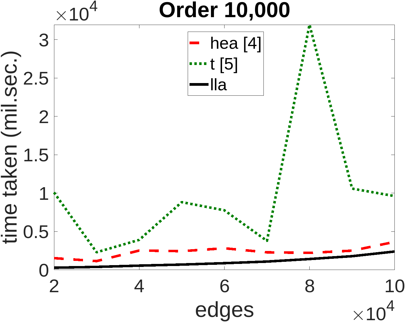
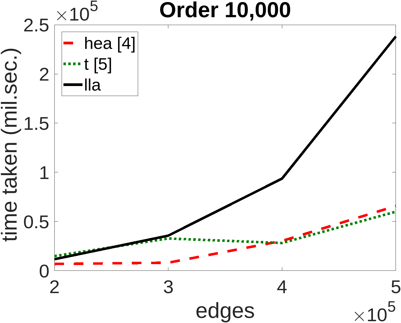
Figure 5: Dominating set algorithms – comparison between runtime of and number of moves taken by Hedetniemi et al. (2003) [4], Turau (2007) [5] and Algorithm 2. All graphs are of 10,000 nodes. (a) Time taken to converge: 20,000 to 100,000 edges. (b) Time taken to converge: 200,000 to 500,000 edges.

In Figure 5 (a) and (b), we present the time taken for computing dominating set on random graphs of 10,000 nodes, 20,000 to 100,000 edges (average degree 4 to 20) and 200,000 to 500,000 edges (average degree 40 to 100) respectively. All graphs are generated by the networkx library of python3. $i[st]$ value ($IN$ or $OUT$) for every node $i$ is initialized randomly. For comparing the performance results, all three algorithms are run on the same set of graphs. All the observations are an average of 3 readings.

The experiments are run in Intel(R) Xeon(R) CPU E5-2670 v2 @ 2.50 GHz, cuda v100s using the gcccuda2019b compiler. The programs are run using the command nvcc $\langle$program$\rangle$.cu -G. In a shared memory model such as cuda, we do not see a loss of time due to the transfer of information. This is because any node can read the data of another node directly. In our implementations, the program for Algorithm 2 was run asynchronously, and the algorithms in [4] and [5] are implemented under the required synchronization model. For the readings, each multiprocessor ran 256 threads. Every thread ran one node at a time.

It can be observed that in sparse graphs, Algorithm 2 takes comparatively less time to converge (cf. Figure 5 (a)). However, as we increase the edge density of the graphs, we observe that the time taken by Algorithm 2 increases (cf. Figure 5 (b)). This is because the time complexity of each guard evaluation in Algorithm 2 is $O(\Delta^{4})$, which is higher than the algorithms presented in [4] and [5]. It follows that a direct implementation of Algorithm 2 will benefit in terms of convergence time in distributed systems where the time taken for the transfer of information is a major issue.

XI Conclusion

Induction of a total order among the local states, which in turn, induces latttice structure among the global states, ensures that (1) in any suboptimal global state, impedensable nodes can be identified distinctly, and (2) for any impedensable node, the local state that it transitions to can be computed. This implies that the final optimal state can be predicted from the initial state. If the problem does not provide a lattice structure, then it can be induced algorithmically, which we demonstrate in this paper: we introduce fully lattice-linear algorithms.

The induction of lattice allows algorithms to execute in asynchrony [2], where reading old values is permitted. We bridge the gap between lattice-linear problems [2] and eventually lattice-linear algorithms [3]. Fully lattice-linear algorithms can be developed even for problems that are not lattice-linear. This overcomes a key limitation of [2] where the model renders ineffective if nodes cannot be deemed impedensable naturally. Since the lattice structures exist in the entire (reachable) state space, we overcome a limitation of [3] where lattices are induced among only a subset of global states.

We analyzed the time complexity bounds of an arbitrary algorithm traversing a lattice of states (whether present naturally in the problem or imposed by the algorithm).

Finally, the approach used for dominating set and colouring cannot be used for all graph algorithms. We explain on this in the Appendix.

Why a similar approach for VC and IS is not lattice-linear?

Here, we elaborate on why the design of lattice-linear algorithms for dominating set and graph colouring that we present in this paper cannot be extended to algorithms for vertex cover and independent set.

We can use the macros $addable$ (some edge of that node is not covered) and $removable$ (removing the node preserves the vertex cover) for the vertex cover problem to design an algorithm for minimal vertex cover. Unfortunately, this solution cannot be converted into a lattice-linear algorithm. This can be observed on a line graph of 4 nodes (numbered 1-4) where all nodes are initialized to $OUT$. Here, node 4 can change its state to $IN$. Other nodes cannot change their state because they have a neighbour with a higher ID that can enter the vertex cover. After node 4 enters the vertex cover, node 3 can enter the vertex cover, as edge $\{2,3\}$ is not covered. However, this requires that node 4 has to leave the vertex cover to keep it minimal. This is not permitted in lattice-linear algorithms, where the local states of a node must form a total order.

A similar behaviour can be observed by an algorithm for independent set on a path of 4 nodes, all initialized to be $IN$.

References

- [1] A. T. Gupta and S. S. Kulkarni, “Brief announcement: Fully lattice linear algorithms,” in Stabilization, Safety, and Security of Distributed Systems, S. Devismes, F. Petit, K. Altisen, G. A. Di Luna, and A. Fernandez Anta, Eds. Cham: Springer International Publishing, 2022, pp. 341–345.
- [2] V. K. Garg, Predicate Detection to Solve Combinatorial Optimization Problems. New York, NY, USA: Association for Computing Machinery, 2020, p. 235–245. [Online]. Available: https://doi.org/10.1145/3350755.3400235
- [3] A. T. Gupta and S. S. Kulkarni, “Extending lattice linearity for self-stabilizing algorithms,” in Stabilization, Safety, and Security of Distributed Systems, C. Johnen, E. M. Schiller, and S. Schmid, Eds. Cham: Springer International Publishing, 2021, pp. 365–379.
- [4] S. Hedetniemi, S. Hedetniemi, D. Jacobs, and P. Srimani, “Self-stabilizing algorithms for minimal dominating sets and maximal independent sets,” Computers & Mathematics with Applications, vol. 46, no. 5, pp. 805–811, 2003. [Online]. Available: https://www.sciencedirect.com/science/article/pii/S089812210390143X
- [5] V. Turau, “Linear self-stabilizing algorithms for the independent and dominating set problems using an unfair distributed scheduler,” Information Processing Letters, vol. 103, no. 3, pp. 88–93, 2007. [Online]. Available: https://www.sciencedirect.com/science/article/pii/S0020019007000488
- [6] V. K. Garg, “A lattice linear predicate parallel algorithm for the housing market problem,” in Stabilization, Safety, and Security of Distributed Systems, C. Johnen, E. M. Schiller, and S. Schmid, Eds. Cham: Springer International Publishing, 2021, pp. 108–122.
- [7] V. Garg, “A lattice linear predicate parallel algorithm for the dynamic programming problems,” in 23rd International Conference on Distributed Computing and Networking, ser. ICDCN 2022. New York, NY, USA: Association for Computing Machinery, 2022, p. 72–76. [Online]. Available: https://doi.org/10.1145/3491003.3491019
- [8] Z. Xu, S. T. Hedetniemi, W. Goddard, and P. K. Srimani, “A synchronous self-stabilizing minimal domination protocol in an arbitrary network graph,” in Distributed Computing - IWDC 2003, S. R. Das and S. K. Das, Eds. Berlin, Heidelberg: Springer Berlin Heidelberg, 2003, pp. 26–32.
- [9] W. Goddard, S. T. Hedetniemi, D. P. Jacobs, P. K. Srimani, and Z. Xu, “Self-stabilizing graph protocols,” Parallel Processing Letters, vol. 18, no. 01, pp. 189–199, 2008. [Online]. Available: https://doi.org/10.1142/S0129626408003314
- [10] W. Y. Chiu, C. Chen, and S.-Y. Tsai, “A 4n-move self-stabilizing algorithm for the minimal dominating set problem using an unfair distributed daemon,” Information Processing Letters, vol. 114, no. 10, pp. 515–518, 2014. [Online]. Available: https://www.sciencedirect.com/science/article/pii/S0020019014000702
- [11] A. Bhartia, D. Chakrabarty, K. Chintalapudi, L. Qiu, B. Radunovic, and R. Ramjee, “Iq-hopping: Distributed oblivious channel selection for wireless networks,” in Proceedings of the 17th ACM International Symposium on Mobile Ad Hoc Networking and Computing, ser. MobiHoc ’16. New York, NY, USA: Association for Computing Machinery, 2016, p. 81–90. [Online]. Available: https://doi.org/10.1145/2942358.2942376
- [12] A. Checco and D. J. Leith, “Fast, responsive decentralized graph coloring,” IEEE/ACM Transactions on Networking, vol. 25, no. 6, pp. 3628–3640, 2017.
- [13] K. R. Duffy, C. Bordenave, and D. J. Leith, “Decentralized constraint satisfaction,” IEEE/ACM Transactions on Networking, vol. 21, no. 4, pp. 1298–1308, 2013.
- [14] K. R. Duffy, N. O’Connell, and A. Sapozhnikov, “Complexity analysis of a decentralised graph colouring algorithm,” Inf. Process. Lett., vol. 107, no. 2, p. 60–63, jul 2008. [Online]. Available: https://doi.org/10.1016/j.ipl.2008.01.002
- [15] S. F. Galán, “Simple decentralized graph coloring,” Computational Optimization and Applications, vol. 66, no. 1, pp. 163–185, Jan 2017. [Online]. Available: https://doi.org/10.1007/s10589-016-9862-9
- [16] D. J. Leith and P. Clifford, “Convergence of distributed learning algorithms for optimal wireless channel allocation,” in in Proceedings of IEEE Conference on Decision and Control, 2006, pp. 2980–2985.
- [17] A. Motskin, T. Roughgarden, P. Skraba, and L. Guibas, “Lightweight coloring and desynchronization for networks,” in IEEE INFOCOM 2009, 2009, pp. 2383–2391.
- [18] D. Chakrabarty and P. de Supinski, On a Decentralized -Graph Coloring Algorithm. Symposium on Simplicity in Algorithms (SOSA), SIAM, 2020, pp. 91–98. [Online]. Available: https://epubs.siam.org/doi/abs/10.1137/1.9781611976014.13