Reinforcement Learning with Large Action Spaces
for Neural Machine Translation

Abstract

Applying Reinforcement learning (RL) following maximum likelihood estimation (MLE) pre-training is a versatile method for enhancing neural machine translation (NMT) performance. However, recent work has argued that the gains produced by RL for NMT are mostly due to promoting tokens that have already received a fairly high probability in pre-training. We hypothesize that the large action space is a main obstacle to RL’s effectiveness in MT, and conduct two sets of experiments that lend support to our hypothesis. First, we find that reducing the size of the vocabulary improves RL’s effectiveness. Second, we find that effectively reducing the dimension of the action space without changing the vocabulary also yields notable improvement as evaluated by BLEU, semantic similarity, and human evaluation. Indeed, by initializing the network’s final fully connected layer (that maps the network’s internal dimension to the vocabulary dimension), with a layer that generalizes over similar actions, we obtain a substantial improvement in RL performance: 1.5 BLEU points on average.

1 Introduction

The standard training method for sequence-to-sequence tasks, specifically for NMT is to maximize the likelihood of a token in the target sentence, given a gold standard prefix (henceforth, maximum likelihood estimation or MLE). However, despite the strong performance displayed by MLE-trained models, this token-level objective function is limited in its ability to penalize sequence-level errors and is at odds with the sequence-level evaluation metrics it aims to improve. One appealing method for addressing this gap is applying policy gradient methods that allow incorporating non-differentiable reward functions, such as the ones often used for MT evaluation (Shen et al., 2016, see §2). For brevity, we will refer to these methods simply as RL.

The RL training procedure consists of several steps: (1) generating a translation with the pre-trained MLE model, (2) computing some sequence-level reward function, usually, one that assesses the similarity of the generated translation and a reference, and (3) updating the model so that its future outputs receive higher rewards. The method’s flexibility, as well as its ability to address the exposure bias (Ranzato et al., 2016; Wang and Sennrich, 2020), makes RL an appealing avenue for improving NMT performance. However, a recent study (C19; Choshen et al., 2019) suggests that current RL practices are likely to improve the prediction of target tokens only where the MLE model has already assigned that token a fairly high probability.

In this work, we observe that one main difference between NMT and other tasks in which RL methods excel is the size of the action space. Typically, the size of the action space in NMT includes all tokens in the vocabulary, usually tens of thousands. By contrast, common RL settings have either small discrete action spaces (e.g., Atari games (Mnih et al., 2013)), or continuous action spaces of low dimension (e.g., MuJoCo (Todorov et al., 2012) and similar control problems). Intuitively, RL takes (samples) actions and assesses their outcome, unlike supervised learning (MLE) which directly receives a score for all actions. Therefore, a large action space will make RL less efficient, as individual actions have to be sampled in order to assess their quality. Accordingly, we experiment with two methods for decreasing the size of the action space and evaluate their impact on RL’s effectiveness.

We begin by decreasing the vocabulary size (or equivalently, the number of actions), conducting experiments in low-resource settings on translating four languages into English, using BLEU both as the reward function and the evaluation metric. Our results show that RL yields a considerably larger performance increase (about $1$ BLEU point on average) over MLE training than is achieved by RL with the standard vocabulary size. Moreover, our findings indicate that reducing the size of the vocabulary can improve upon the MLE model even in cases where it was not close to being correct. See §4.

However, in some cases, it may be undesirable or unfeasible to change the vocabulary. We therefore experiment with two methods that effectively, reduce the dimensionality of the action space without changing the vocabulary. We note that generally in NMT architectures, the dimensionality of the decoder’s internal layers (henceforth, $d$) is significantly smaller than the target vocabulary size (henceforth, $|V_{T}|$), which is the size of the action space. A fully connected layer is generally used to map the internal representation to suitable outputs. We may therefore refer to the rows of the matrix (parameters) of this layer, as target embeddings, mapping the network’s internal low-dimensional representation back to the vocabulary size, the actions. We use this term to underscore the analogy between the network’s first embedding layer, mapping vectors of dimension $|V_{T}|$ to vectors of dimension $d$, and target embeddings that work in an inverse fashion. Indeed, it is often the case (e.g., in BERT, Devlin et al., 2019) that the weights of the source and target embeddings are shared during training, emphasizing the relation between the two.

Using this terminology, we show in simulations (§5.1) that when similar actions share target embeddings, RL is more effective. Moreover, when target embeddings are initialized based on high-quality embeddings (BERT’s in our case), freezing them during RL yields further improvement still. We obtain similar results when experimenting on NMT. Indeed, using BERT’s embeddings for target embeddings improves performance on the four language pairs, and freezing them yields an additional improvement on both MLE and RL as reported by both automatic metrics and human evaluation. Both initialization and freezing are novel in the context of RL training for NMT. Moreover, when using BERT’s embeddings, RL’s ability to improve performance on target tokens to which the pre-trained MLE model did not assign a high probability, is enhanced (§5.2).

2 Background

2.1 RL in Machine Translation

RL is used in text generation (TG) for its ability to incorporate non-differentiable signals, to tackle the exposure bias, and to introduce sequence-level constraints. The latter two are persistent challenges in the development of TG systems, and have also been addressed by non-RL methods (e.g., Zhang et al., 2019; Ren et al., 2019). In addition, RL is grounded within a broad theoretical and empirical literature, which adds to its appeal.

These properties have led to much interest in RL for TG in general (Shah et al., 2018) and NMT in particular (Wu et al., 2018a). Numerous policy gradient methods are commonly used, notably REINFORCE (Williams, 1992), and Minimum Risk Training (MRT; e.g., Och, 2003; Shen et al., 2016). However, despite increasing interest and strong results, only a handful of works studied the source of observed performance gains by RL in NLP and its training dynamics, and some of these have suggested that RL’s gains are partly due to artifacts (Caccia et al., 2018; Choshen et al., 2019).

In a recent paper, C19 showed that existing RL training protocols for MT (REINFORCE and MRT) take a prohibitively long time to converge. Their results suggest that RL practices in MT are likely to improve performance only where the MLE parameters are already close to yielding the correct translation. They further suggest that observed gains may be due to effects unrelated to the training signal, but rather from changes in the shape of the distribution curve. These results may suggest that one of the drawbacks of RL is the uncommonly large action space, which in TG includes all tokens in the vocabulary, typically tens of thousands of actions or more.

To the best of our knowledge, no previous work considered the challenge of large action spaces in TG, and relatively few studies considered it in different contexts. One line of work assumed prior domain knowledge about the problem, and partitioned actions into sub-groups (Sharma et al., 2017), or similar to our approach, embedding actions in a continuous space where some metric over this space allows generalization over similar actions (Dulac-Arnold et al., 2016). More recent work proposed to learn target embeddings when the underlying structure of the action space is apriori unknown using expert demonstrations (Tennenholtz and Mannor, 2019; Chandak et al., 2019).

This paper establishes that the large action spaces are a limiting factor in the application of RL for NMT, and propose methods to tackle this challenge. Our techniques restrict the size of the embedding space, either explicitly or implicitly by using an underlying continuous representation.

2.2 Technical Background and Notation

Notation.

We denote the source sentence with $X=(x_{1},...,x_{S})$ and the reference sentence with $Y=(y_{1},...,y_{T})$. Given $X$, the network generates a sentence in the target language $Y^{\prime}=(y^{\prime}_{1},...,y^{\prime}_{M})$. Target tokens are taken from a vocabulary $V_{T}$. During inference, at each step $i$, the probability of generating a token $y^{\prime}_{i}\in V_{T}$ is conditioned on the sentence and the predicted tokens, i.e., $P_{\theta}(y^{\prime}_{i}|X,y^{\prime}_{<i})$, where $\theta$ is the model parameters. We assume there is exactly one valid target token, the reference token, as in practice, training is done against a single reference (Schulz et al., 2018).

NMT with RL.

In RL terminology, one can think of an NMT model as an agent, which interacts with the environment. In this case, the environment state consists of the previous words $y^{\prime}_{<i}$ and the source sentence $X$. At each step, the agent selects an action according to its policy, where actions are tokens. The policy is defined by the parameters of the model, i.e., the conditional probability $P_{\theta}(y^{\prime}_{i}|y^{\prime}_{<i},X)$. Reward is given only once the agent generates a complete sequence $Y^{\prime}$. The standard reward for MT is the sentence level BLEU metric (Papineni et al., 2002), matching the evaluation metric. Our goal is to find the parameters that will maximize the expected reward.

In this work, we use MRT (Och, 2003; Shen et al., 2015), a policy gradient method adapted to MT. The key idea of this method is to optimize at each step a re-normalized risk, defined only over the sampled batch. Concretely, the expected risk is defined as:

$$L_{risk}=\sum_{u\in U(X)}R(Y,u)\frac{P(u|X)^{\beta}}{\sum_{u^{\prime}\in U(X)}P(u^{\prime}|X)^{\beta}}$$ (1)

where $u$ is a candidate hypothesis sentence, $U(x)$ is the sample of $k$ candidate hypotheses, $Y$ is the reference, $P$ is the conditional probability that the model assigns a candidate hypothesis $u$ given source sentence $X$, $\beta$ a smoothness parameter and $R$ is BLEU.

3 Methodology

Architecture.

We use a similar setup as used by Wieting et al. (2019), adapting their fairSeq-based (Ott et al., 2019) codebase to our purposes. Similar to their Transformer architecture we use gated convolutional encoders and decoders (Gehring et al., 2017). We use 4 layers for the encoder and 3 for the decoder, the size of the hidden state is 768 for all layers, and the filter width of the kernels is 3. Additionally, the dimension of the BPE embeddings is set to 768.

Data Prepossessing.

We use BPE (Sennrich et al., 2016) for tokenization. The vocabulary size is set to 40K for the combined source and target vocabulary as done by Wieting et al. (2019). For the small target vocabulary experiments, we change the target vocabulary size to 1K and keep the source vocabulary unchanged.

Objective Functions.

Following Edunov et al. (2018), we train models with MLE with label-smoothing (Szegedy et al., 2016; Pereyra et al., 2017) of size 0.1. For RL, we fine-tune the model with a weighted average of the MRT $L_{risk}$ and the token level loss $L_{mle}$.

Our fine-tuning objective thus becomes:

$$L_{Average}=\alpha\cdot L_{mle}+(1-\alpha)\cdot L_{risk}$$ (2)

We set $\alpha$ to be 0.3 shown to work best by Wu et al. (2018b). We set $\beta$ to 1. We generate eight hypotheses for each MRT step ($k$=8) with beam search. We train with smoothed BLEU (Lin and Och, 2004) from the Moses implementation. Moreover, we use this metric to report results and verify they match sacrebleu (Post, 2018).

Optimization.

We train the MLE objective over 200 epochs and the combined RL objective over 15. We perform early stopping by selecting the model with the lowest validation loss. We optimize with Nesterov’s accelerated gradient method (Sutskever et al., 2013) with a learning rate of 0.25, a momentum of 0.99, and re-normalize gradients to a 0.1 norm (Pascanu et al., 2012).

Data.

We experiment with four languages: German (De), Czech (Cs), Russian (Ru), and Turkish (Tr), translating each of them to English (En). For training data for cs-en, de-en, and ru-en, we use the WMT News Commentary v13 (Bojar et al., 2017). For tr-en training data, we use WMT 2018 parallel data, which consists of the SETIMES2 corpus (Tiedemann, 2012). The validation set is a concatenation of newsdev 2016 and 2017 released for WMT18. Test sets are the official WMT18 test sets. Those experiments focus on a low-resource setting. We choose this setting as RL experiments are computationally demanding and this setting is common in the literature for RL experiments like ours Wieting et al. (2019). (see data statistics in Supp. §A)

4 Reducing the Vocabulary Size

We begin by directly testing our hypothesis that the size of the action space is a cause for the long convergence time of RL for NMT. To do so, we train a model with target-side BPE taken from a much smaller vocabulary than is typically used.

We begin by training two MLE models, one with a large (17K-31K) target vocabulary (LTV) and another with a target vocabulary of size 1K (STV). The source vocabulary remains unchanged. We start with the MLE pretraining and then train each of the two models with RL.

Results (Table 1) show that the RL training with STV achieves about $1$ BLEU point more than the RL training with LTV. For a comparison of the models’ entropy see Supp. §B. In order to verify that the improvement does not stem from the choice of $\alpha$ mixing RL and MLE (see Eq. 2), we repeat the training for De-En with $\alpha\in\{0,1\}$, we find that $\alpha=0.3$ is superior to both. Moreover, RL improves STV more than LTV when training with only the RL objective ($\alpha=1$). This indicates that RL training contributes to the observed improvement.

Model	DE-EN	CS-EN	RU-EN	TR-EN
LTV	25.07	15.16	16.67	12.76
LTV+RL	25.67	15.33	16.9	12.98
Diff.	0.6	0.17	0.23	0.22
STV	21.83	13.79	14.63	10.37
STV+RL	23.23	14.62	15.73	11.96
Diff.	1.4	0.83	1.1	1.59

Table 1: BLEU scores for translating four languages to English using MLE pretraining followed by RL, and comparing a model with a large vocabulary (LTV) to a small one (STV). The top (bottom) block presents results for LTV (STV) with and without RL, and the difference between them (Diff.). RL with STV gains more than 1 point more (on average) over the pre-trained MLE model, than RL with LTV.

We next turn to analyze what tokens are responsible for the observed performance gain. Specifically, we examine whether reducing the vocabulary size resulted in RL being able to promote target tokens that received a low rank by the pre-trained MLE model. For each model, for 700K trials, we compute what rank the model assigns to the gold token $y_{i}$ for a context $y^{\prime}_{<i}$ and source sentence $X$. Formally, $\forall r\in|V_{T}|$, $P^{r}_{model}=\frac{\#\{gold\ token\ assigns\ to\ the\ r\ rank\}}{\#\{all\ trials\}}$. We then compare the rank distribution of the MLE model to that of the RL model by subtracting those two distributions. In our notation, for each rank r, $\Delta P^{r}=P^{r}_{RL}-P^{r}_{MLE}$. This subtraction represents how RL influences the model’s ability to assign the correct token $y_{i}$ for each rank. The greater the positive effect of RL is, the more probable it is that the probability will be positive for the first rank, and negative for lower ranks (due to the probability shift to first place).

Figure 1 presents the probability difference per rank for LTV and STV. We can see that for the first rank the probability shift due to RL training with STV is more than twice the shift caused by RL training with LTV. Consequently, the probability shift for the following ranks is usually more negative for small vocabulary settings. The figure indicates that indeed the shift of probability mass to higher positions occurs substantially more when we apply RL using a smaller action space. Moreover, the STV training was able to shift probability mass from lower ranks upwards compared to LTV. An indication for that is that, within the first one hundred ranks, STV reduces the probability of $83$ of them, whereas LTV of only $2$.

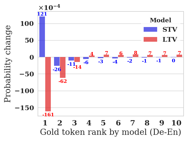
Figure 1: Comparison of probability shift due to RL training of assign $y_{best}$ for ten first words for both LTV and STV. in blue, you can see the results with BPE of size 1,000, STV. in red are the results with BPE of size 30,000, LTV. a clear improvement of assigning $y_{best}$ in first place for STV.

5 Reducing the Effective Dimensionality of the Action Space

Finding that reducing the number of actions improves RL’s performance, we propose a method for reducing the effective number of actions, without changing the actual output. The vocabulary size might be static, as in pre-trained models (Devlin et al., 2019), and reducing it might help RL but be sup-optimal for MLE (Gowda and May, 2020), or introduce out-of-domain words (Koehn and Knowles, 2017). We propose to do so by using target embeddings that generalize over tokens that appear in similar contexts. We explore two implementations of this idea, one where we initialize the target embeddings with high-quality embeddings, and another where we freeze the learned target embeddings during RL. We also explore a combination of the two approaches. Freezing the target embeddings (decoder’s last layer) can be construed as training the network to output the activations of the penultimate layer, where a fixed function then maps it to the dimension of the vocabulary.

We note that although freezing is a common procedure (Zoph et al., 2016; Thompson et al., 2018; Lee et al., 2019; Coster et al., 2021), as far as we know, it has never been applied in the use of RL for sequence to sequence models.

Denote the function that the network computes with $f_{\theta}$. $f_{\theta}$ can be written as $h_{\theta_{2}}\circ g_{\theta_{1}}$, where $\theta=\left(\theta_{1},\theta_{2}\right)$, $g$ maps the input – source sentence $X$ and model translation prefix $y^{\prime}_{<i}$ – into $\mathbb{R}^{d}$, and $h$ maps $g$’s output into $\mathbb{R}^{|V_{T}|}$.

Using this notation, we can formulate the method as loading pre-trained MLE target embeddings to $h_{\theta_{2}}$ or freezing it (or both). As for many encoder-decoder architectures (including the Transformer), it holds that $d\ll|V_{T}|$, this can be thought of as constraining the agent to select a $d$-dimensional continuous action, where $h_{\theta_{2}}$ is a known transformation performed by the environment.

The importance of target embedding is that they allow for better generalization over actions. The intuition is as follows. Assume two tokens have the same embedding, and similar semantics, i.e., they are applicable in the same contexts (synonyms). Since they have the same target embeddings, during training the network will perform the same gradient updates when encountering either of them, except for in the last layer (since they are still considered different outputs). If the target embeddings are not frozen, encountering either of them during training will lead to very similar updates (since they have the same target embeddings), but their target embeddings may drift slightly apart, which will cause a subsequent drift in the lower layers. If the target embeddings are frozen, the gradient updates they will yield will remain the same and expedite learning. We hypothesize a similar effect during training, where tokens that have similar (but not identical) embeddings, and a similar (but not identical) distribution would benefit in training from each other. This motivates us to explore a combination of informative initialization and parameter freezing. (see formal proof in Supp. §E).

5.1 Motivating Simulation through Policy Parameterization in Large Action Spaces

In order to examine the intuition outlined above in a controlled setting, we consider a synthetic RL problem in which the action space is superficially enlarged. The task is a (contextual) multi-armed-bandit, with $K$ actions. At each step, an input state is sampled from the environment (the "context"; a random vector sampled from a multivariate Gaussian distribution). A random, fixed, non-linear binary classifier determines whether action #1 or action #2 is rewarding based on the given context (actions $3$-$K$ are never rewarding), and the reward for each action is $r+z$ where $r=1$ for the rewarding action and $0$ for all other actions, and $z\sim\mathcal{N}\left(0,0.1\right)$. Crucially, we duplicate each action $a$ times, resulting in a total of $K\times a$ actions at the policy level – whereas for the environment all ‘copies’ of a given action are equivalent.

The problem structure, including the classifier itself, is unknown to the RL agent, which directly optimizes a policy parameterized as a fully-connected feed-forward neural network. We control two aspects of the last layer of the policy network, resulting in a total of four variants of agents. First, the last layer can be frozen to its initial value, or learned (by RL). Second, the last layer can be initialized at random, or induce a prior regarding the duplicated actions (such that weight vectors projecting to different copies of a given action are initialized identically). We call the latter the informative initialization.

We stress that the informative initialization carries no information about the underlying reward structure of the problem (i.e., the classifier, and the identity of the rewarding actions), but only as to which actions are duplicated. Nevertheless, as shown in Figure 2, a prior regarding the structure of the action space is helpful on its own, leading to faster learning (compare Informative to Full net).

Results fit the intuition presented. With informative last layer initialization, learning in previous layers generalizes over the duplicated actions and boosts early stages of learning, leading to faster convergence. We note that in this setting faster learning is not only the result of learning fewer parameters. Notably, freezing the last layer with random initialization, prohibits the network from learning the task. This is due to the regime of a very large action space (output layer; width $4000$) compared to the dimensionality of the hidden representations (width $300$). Freezing an informative initialization, on the other hand, sets the network in a rather different regime, in which the effective size of the output layer is (much) smaller than the hidden representation (i.e #‘real’ actions; 10). In this regime, the network is generally expressive enough so that it can quickly learn the task even with a fixed, random readout layer (Hoffer et al., 2018).

To conclude, this example provides evidence that initializing and possibly freezing the last layer in the policy network in a way that respects the structure of the action space is helpful for learning in vast action spaces, as it supports generalization over similar or related actions. Importantly, this helps even when the (frozen) initialization does not contain task-specific information. In a more realistic scenario, actions are not simply a complete duplicate of each other, but rather are organized in some complex structure. Informative initialization, then, accounts not for duplicating weights, but for initializing them in such a way that a-priori reflects, or is congruent, with this structure. This motivates our approach – in the realistic, complicated task of MT – to freeze a learned output layer for the policy network, from a model whose embeddings have been shown to be effective across a wide range of tasks (in our case, BERT).

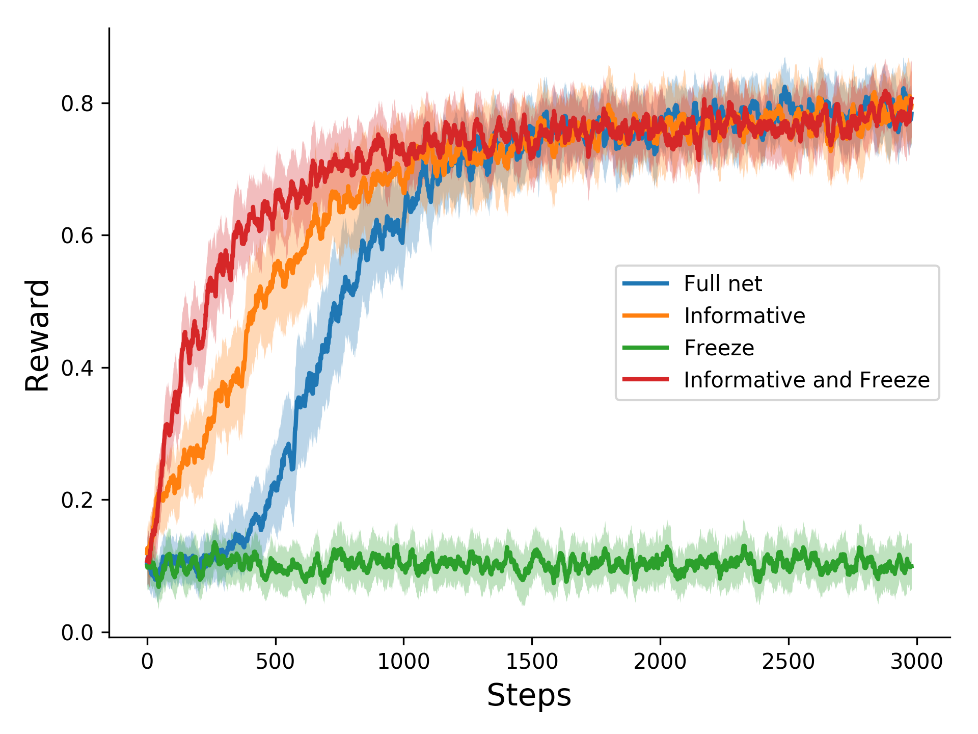
Figure 2: Simulating learning in large action spaces. Figures show a moving average over $20$ steps of the underlying binary reward. Solid curves denote mean, shaded area denote $\pm 0.5$ s.d. ($N=50$ trials per agent, $K=10,a=400$, network architecture: 10-300-300-4000). Informative initialization is effective on its own, and more so when freezing is applied.

5.2 NMT Experiments

The motivating analysis and simulations indicate that it is desirable to use target embeddings that assign similar values to similar actions. Doing so can be viewed as an effective reduction in the dimensionality of the action space. We turn to experiment with this approach on NMT. We explore two approaches: (1) freezing $h$ during RL; (2) informatively initializing $h$, as well as their combination. Our main results are presented in Table 2.

As a baseline, we experiment with freezing uninformative target embeddings: target embeddings are randomly initialized and frozen during both MLE and RL. Unsurprisingly, doing so does not help training, and in fact, greatly degrades it (in about 2 BLEU points in En-De).

Next, we examine whether the target embeddings of the MLE pretraining are informative enough, namely whether freezing them during RL leads to improved effectiveness. Results show a slight improvement in BLEU when doing so, which is encouraging given that the frozen embeddings’ weights consist of more than half of the network’s trainable parameters. Indeed, freezing the embedding layers has a dramatic impact on the volume of trainable parameters, decreasing their size by more than $60\%$. In Supp. §D we present the number of trainable parameters in each setting.

We therefore hypothesize that, as in the simulations (§5.1), the quality of the frozen embedding space is critical for the success of this approach. As using frozen MLE embeddings improves performance, but only somewhat, we further consider target embeddings that were trained on much larger datasets, specifically BERT’s embedding layer.

For this set of experiments, we adjust the target vocabulary to be BERT’s vocabulary of size $|V_{T}|=30526$. We train RL models with and without freezing the embedding layers and with and without loading BERT embedding. We report results of MLE training with BERT’s embedding when the embedding is kept frozen as it reaches superior results (see Supp. §C).

The results (Table 2) directly parallels our findings in the simulations: Initializing from BERT ($+BERT+RL$) improves performance across all language pairs, and freezing ($+RL+FREEZE$) yields an additional improvement in most settings, albeit a more modest one. Combining both methods provides additional improvement. Indicating that FREEZE and BERT are helpful both independently and in conjunction. In total, our model ($+BERT+RL+FREEZE$) achieves $1.5$ BLEU points improvements over regular $RL$. We also report semantic similarity scores in Supp. §F.

Notably, our method surpasses the LTV+RL results (Table 1) across all languages except German, overall about 1.5 BLEU points more on average. We hypothesize that the reason for this degradation is the lower results of the MLE with BERT’s vocabulary compared to the joint BPE vocabulary which is known to be superior to BPE on each language individually, especially when the source and target languages are close (Sennrich et al., 2016). These considerations are peripheral to our discussion, which specifically targets the effectiveness of the RL approach.

Finally, initializing from BERT increases RL’s ability to promote tokens that were not ranked high according to the MLE model (Fig. 3).

MODEL	De-En	Cs-En	Ru-En	Rr-En
MLE	22.38	15.81	17.31	12.60
+RL	23.19	15.81	17.31	12.66
+RL+FREEZE	23.14	16.04	17.78	13.18
+BERT	23.46	16.59	18.14	14.15
+BERT+RL	24.44	17.04	18.68	14.37
+BERT+RL+FREEZE	24.71	17.37	18.30	14.55

Table 2: BLEU scores on translating four languages to English. The upper block shows the baseline scores of training only with MLE, and with MLE followed by RL. RL presents modest improvement (if any) over only using MLE. +RL+FREEZE shows some improvement due to freezing the target embeddings. The lower three rows show results when using BERT’s target embeddings (informative initialization). Additional benefit is seen from freezing (+RL+BERT+FREEZE).

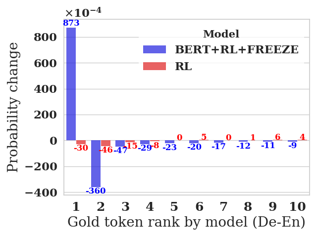
Figure 3: Comparison of the change in the rank distribution of the target token following RL in two settings, one where RL training with frozen BERT embeddings is used (blue) and the second when we used basic RL training (red). The gain in probability in the first rank indicates that the model is more probable to be correct (which is reflected in its superior performance over the pre-trained MLE model). The negative values in the following places demonstrate how RL with frozen high-quality target embeddings can improve not only when the MLE model is initially close to being correct.

6 Human Evaluation

We perform human evaluation, comparing the baseline $RL$ with our proposed model. We selected 100 translations from the respective test sets of each language. The annotation was performed by two professional annotators (contractors of the project), who work in the field of translation. Both are native English speakers. The annotators assigned a score from 0 to 100, judging how well the translation conveyed the information contained in the reference (see annotation guidelines in Supp. §G). From Fig. 4, we see that our proposed model scores the highest across all language pairs. To test statistical significance, we use the Wilcoxon rank sum test to standardize score distributions fit for our setting (Graham et al., 2015). Comparing the two models’ distributions, we got a p-value of $8.5e^{-5}$ indicating the improvement is significant. We emphasize that our main goal is showing that our method can improve the optimized metric (e.g., BLEU), and hence the improvement over the semantic similarity score and the human evaluation is an additional indication of our method’s robustness.

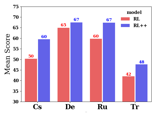
Figure 4: Average human ratings on 200 sentences from the test set for each of the respective languages. $RL$ is the baseline RL model and $RL++$ is our model ($+BERT+RL+FREEZE$). The performance of our model is consistently better than the baseline.

7 Comparing Target Embedding Spaces

The previous section discussed how BERT’s target embeddings improve RL performance, compared to target embeddings learned by MLE. We now turn to directly analyze the generalization ability of the two embeddings. We do so by comparing the embeddings of semantically related words.

We use WordNet (Miller, 1998) and spaCy to compile three lists of word pairs: inflections (e.g., ’documentaries’ / ’documentary’, ’boxes’ / ’box’, ’stemming’ / ’stem’), synonyms (e.g., ’luckily’ / ’fortunately’, ’amazement’ / ’astonishment’, ’purposely’ / ’intentionally’), and random pairs, and compare the embeddings assigned to these pairs using BERT and MLE embeddings. Figure 5 presents the distributions of the cosine similarity of the pairs in the three lists for both embedding spaces. Results show that MLE embeddings for the different lists have almost identical distributions, demonstrating the limited informativeness of these target embeddings. In contrast, BERT embeddings only display a small overlap between the similarity distributions of inflections and random pairs. However, synonyms’ distribution remains quite similar to that of random pairs. In conclusion, BERT embeddings better discern semantics overall compared to MLE embeddings, which may partly account for their superior performance. Results also indicate BERT’s embeddings could be further improved.

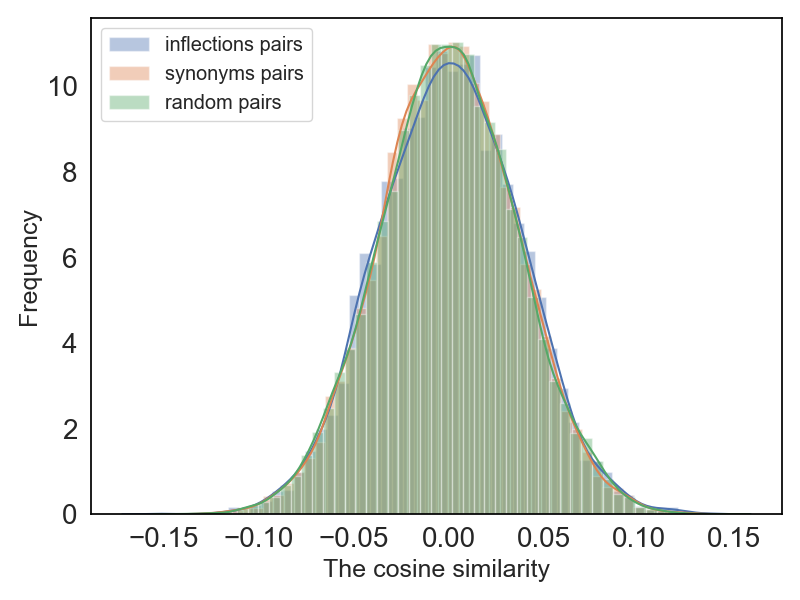
(a) MLE embeddings

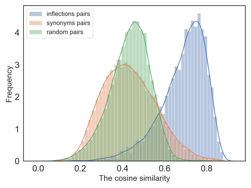
(b) BERT embeddings

Figure 5: Comparison of the distribution of the cosine similarity between word pairs from three groups: random word pairs (in green), synonym pairs that do not share a stem (in orange), and pairs of synonyms that share a stem (in blue). The top figure refers to the target embeddings learned by MLE, and the bottom one to BERT embeddings. The ability of the embeddings to distinguish between these three groups is informative of their ability to map semantically related words to similar embeddings. The better discrimination ability of BERT embeddings is thus likely related to their superiority as target embeddings over MLE embeddings.

8 Conclusion

In this paper, we addressed the limited effectiveness of RL for NMT, seeking to understand its origins and offer means for tackling it. We hypothesized that this limitation arises from the size of the action spaces used in NMT and examined two ways of reducing their effective dimension. In the first method, we experiment with smaller vocabularies, showing improved RL effectiveness. While this method constrains the size of the vocabulary, which may be limiting in some settings (Ding et al., 2019; Gowda and May, 2020), it motivates further research along these lines.

The second approach introduces a new method of using informative target embeddings and potentially freezing them during RL. We find that this method may be beneficial as well, but its effectiveness crucially depends on the quality of the employed embeddings. Indeed, we find using both simulations and NMT experiments that freezing in itself results in some improvement in RL performance, but that combined with target embeddings that generalize over words with a similar distribution, it may yield substantial gains as shown by BLEU, semantic similarity, and human evaluation. We compare the target embeddings produced by MLE and those by BERT, finding the latter to be considerably stronger. Those results in low resources settings, encourage further research aiming to address the problem of large action space for TG in richer data settings by adapting and extending our methods.

Future work will increase the exploration ability of RL training in NMT. A promising line of research towards this goal is using off-policy methods. Off-policy methods, in which observations are sampled from a different policy than the one we currently optimize, are prominent in RL (Watkins and Dayan, 1992; Sutton et al., 1998), and were also studied in the context of policy gradient methods (Degris et al., 2012; Silver et al., 2014). We believe that the adoption of such methods to enhance exploration, combined with our proposed method for using target embeddings, can be a promising path forward for the application of RL in NMT, and more generally in TG.

A different line of future work will focus on changing the network’s architecture to predict a $d$ dimension continuous action, instead of discrete actions. Such an approach may directly reduce the size of the action space without limiting the number of words that can be predicted.

9 Acknowledgements

This work was supported by the Israel Science Foundation (grant no. 2424/21), and by the Applied Research in Academia Program of the Israel Innovation Authority.

Appendix A Methodology

Table 3 present the train, validation and test sizes in all four languages pairs. We note that our use of the data is aligned with the license and intended use of the data.

Lang.	Train	Valid	Test
de-en	284,246	6,003	2,998
cs-en	218,384	6,004	2,983
ru-em	235,159	5,999	3,000
tr-en	207,678	6,007	3,000

Table 3: Number of sentence pairs in the training/validation/test sets for all four languages.

Appendix B Entropy of STV and LTV

As C19 suggested we can compare the peakiness of the two models by calculating their distributions entropy. Lower entropy indicates a more peaky distribution. We used KL divergence with respect to the uniform distribution in order to normalize the entropy and compare the peakiness of the two models. The STV model starts RL training with mean entropy of 0.300 and finishes with 0.269 while the LTV begins with 0.258 and finishes with 0.264. This indicates that before RL training the LTV model was slightly more peaky than the STV, but after RL training they have similar peakiness.

Appendix C Loading Bert embedding

We consider two options for initializing Bert embeddings for the MLE training, with and without freezing the embedding layer. The results were unequivocal, freezing the embedding layers has a very constructive effect on the results (table 4). We estimate that freezing the embedding layers causes such a vast improvement in performance because it enables us to avoid the catastrophic forgetting of BERT parameters. Therefore, although using BERT embedding is helpful as initialization, by freezing the parameters we allow the model to better utilize BERT’s embeddings.

Model	De-En	Cs-En	Ru-En	Tr-En
MLE	22.38	15.81	17.31	12.60
MLE+Bert W/o freeze	22.99	15.32	17.57	12.65
MLE+Bert with freeze	23.46	16.59	18.14	14.15
diff.	0.47	1.27	0.57	1.50

Table 4: Comparison of MLE models with BERT embedding with and without freezing.

Appendix D Number of parameters

In Table 5 we provide a comparison of the number of trainable parameters with and without freezing the embedding layer.

# parameters	De-En	Cs-En	Ru-En	Tr-En
Freeze	30.2M	29.3M	27.9M	29.4M
W/o Freeze	77.2M	76.2M	74.8M	76.4M
Ratio	0.39	0.38	0.37	0.38

Table 5: Comparison if trainable parameters.

Appendix E Formalizing the intuition behind freezing the embedding layer

Here we want to formalize the intuition behind freezing the embedding layer. We explicitly calculate the gradients of the cross-entropy (CE) loss of the one-hot vector, $y$, and the distribution vector, $\hat{y}$ of the model $f_{\theta}=h_{\theta_{2}}\circ g_{\theta_{1}}$ output (henceforth, we will discard the parameters notation from $f,g$ and $h$). We will discuss two cases, one when we freeze $\theta_{2}$ and the second when we are not. We note that $\theta_{2}\in\mathbb{R}^{d\times|V_{T}|}$ is the embedding layer where each row, $\rho_{i}$, is the representation of the $k$’s word in the vocabulary. Moreover, $h:\mathbb{R}^{d}\rightarrow\mathbb{R}^{|V_{T}|}$ is the function defined by multiplying the output of $g$, denoted by $v\in\mathbb{R}^{d}$, by $\theta_{2}$, and then taking the soft-max of the output vector, hence $\forall k\in|V_{T}|;h_{k}(v)=\frac{exp(\rho_{k}\cdot v)}{\sum_{l}exp(\rho_{l}\cdot v)}$. Therefore assigning to each word some probability, $\hat{y}_{k}$, to be the next one in the sentence.

Now, we want to investigate the update defined by the gradients of the CE loss in the setting when two words, $w_{1}$ and $w_{2}$ have the same representation, $\rho_{1}=\rho_{2}$. We consider the case where one of them is the gold token, w.l.g. $w_{1}$. We note this case by $\Big{|}^{1}$.

We turn to examine the gradient in this setting for both cases. We start by realizing that if all the partial derivatives of the CE loss, $L$, exist then the gradient is the vector of all the partial derivatives meaning, $\nabla_{\theta}L=\begin{pmatrix}\nabla_{\theta_{1}}L\\ \nabla_{\theta_{2}}L\end{pmatrix}$ and we can separate the calculation into two parts, one with respect to $\theta_{1}$ and the second with respect to $\theta_{2}$.

By definition, in the case where we freeze $\theta_{2}$ we will keep $\rho_{1}$ and $\rho_{2}$ the same. We will now show that in the case when we don’t freeze $\theta_{2}$ the update will be different.

Lemma E.1.

If $\theta_{2}$ is not frozen then: Updates are differe: $\Delta\rho_{1}!=\Delta\rho_{2}$.

Proof.

We start by noticing that multiplying $v$ by $\theta_{2}$ is a linear transformation so for points $p_{1}$ and $p_{2}$ we will get the same derivative as $\rho_{1}=\rho_{2}$, moreover by taking the soft-max of those identical outputs we will get the same outputs. Hence, we get that $\forall i\in[d];\frac{\partial\hat{y}_{1}}{\partial v_{i}}=\frac{\partial\hat{y}_{2}}{\partial v_{i}}$, similarly $\frac{\partial\hat{y}_{1}}{\partial\rho_{1i}}=\frac{\partial\hat{y}_{2}}{\partial\rho_{2i}}$.

We continue by calculating the derivative of the CE. The CE loss is defined by:

$$L(y,\hat{y})=\sum_{i}y_{i}log(\hat{y}_{i})$$ (3)

The derivative is: $\frac{\partial L}{\partial\hat{y}_{i}}=\sum_{i}y_{i}\frac{1}{\hat{y}_{i}}$ we notice that $y$ is a one hot vector i.e., $y_{1}=1$ and $\forall i\in[2,|V_{T}|];y_{i}=0$. Therefore, the derivative will be different from $i=1$ to all other $i$’s. Specifically, $\forall i\in[d];\frac{\partial L}{\partial\rho_{1i}}\neq\frac{\partial L}{\partial\rho_{2i}}$ . Putting it all together we get:

$$\frac{\partial L}{\partial\rho_{1i}}=\frac{\partial L}{\partial\hat{y}_{1}}\cdot\frac{\partial\hat{y}_{1}}{\partial\rho_{1i}}\neq\frac{\partial L}{\partial\hat{y}_{2}}\cdot\frac{\partial\hat{y}_{2}}{\partial\rho_{2i}}=\frac{\partial L}{\partial\rho_{2i}}$$ (4)

Proving that $\rho_{1}$ and $\rho_{2}$ updates are different.

∎

Lemma E.2.

For both cases, the update of $\theta_{1}$ is symmetric to the gold being $w_{1}$ or $w_{2}$. $\nabla_{\theta_{2}}L\Big{|}^{1}=\nabla_{\theta_{2}}L\Big{|}^{2}$.

Proof.

Given a parameter $\lambda\in\theta_{1}$, we inspect the derivative of $L$ with respect to $\lambda$. We use here Einstein summation notation.

$$\frac{\partial L}{\partial\lambda}\Big{|}^{1}=\frac{\partial L}{\partial v_{i}}\cdot\frac{\partial v_{i}}{\partial\lambda}\Big{|}^{1}=\frac{\partial L}{\partial v_{i}}\cdot\frac{\partial v_{i}}{\partial\lambda}\Big{|}^{2}=\frac{\partial L}{\partial\lambda}\Big{|}^{2}$$ (5)

We deduce $\frac{\partial v_{i}}{\partial\lambda}\Big{|}^{1}=\frac{\partial v_{i}}{\partial\lambda}\Big{|}^{2}$, as the derivative of $v_{i}$ is independent of the question which word is the gold. In order to justify the second equality we used, we will write the derivative of $L$ with respect to $v_{i}$.

$$\frac{\partial L}{\partial v_{i}}\Big{|}^{1}=\frac{\partial L}{\partial\hat{y}_{k}}\cdot\frac{\partial\hat{y}_{k}}{\partial v_{i}}$$ (6)

Clearly, we only need to check the elements that change by switching the gold from being $w_{1}$ to $w_{2}$ or vice versa. Therefor all the second terms that multiply by $\frac{\partial L}{\partial\hat{y}_{k}}$ for $k\in[3,|V_{T}|]$ didn’t change. We already proved that $\forall i\in[d];\frac{\partial\hat{y}_{1}}{\partial v_{i}}=\frac{\partial\hat{y}_{2}}{\partial v_{i}}$ Finally, because we switch the gold, $\frac{\partial L}{\partial\hat{y}_{1}}$ and $\frac{\partial L}{\partial\hat{y}_{2}}$ indeed switch there values but both of them are multiply by the same values as $\frac{\partial\hat{y}_{1}}{\partial v_{i}}=\frac{\partial\hat{y}_{2}}{\partial v_{i}}$. Overall, the derivative is unchanged. ∎

To conclude, in the motivational setting we discussed, when we freeze $\theta_{2}$ we keep semantically close vectors unchanged while if we don’t freeze $\theta_{2}$ we enable them to change. As consequence, in further steps, this change will affect on $\theta_{1}$ also. In a similar manner, as long as the representation is similar, all layers but the penultimate would update both words similarly.

Appendix F Semantic scores for the second method

Our method of freezing informative initialization of the embedding layer aims to generalize across different but semantically close actions. In order to test the ability of our model to generalize we used SIM. SIM is a measure of semantic similarity that assigns partial credit to semantically correct but lexically different translations (Wieting et al., 2019). Table 6 shows our model results and exhibits similar trends to the BLEU scours. Here we see even greater gains for cs-en and ru-en languages pairs. Those results may indicate that the model was able to predict tokens that are semantically close to the gold token.

MODEL	De-En	Cs-En	Ru-En	Tr-En
MLE	70.03	63.29	66.17	59.68
+RL	71.17	63.29	66.17	59.99
+RL+FREEZE	71.03	64.29	66.66	60.52
+BERT	71.56	64.26	66.70	61.75
+BERT+RL	72.44	65.80	67.94	63.59
+BERT+RL+FREEZE	72.81	66.44	67.66	63.59

Table 6: SIM scores on translating four languages to English.

Appendix G Human Evaluation Information

We recruited the service of two professional translators via translations providers.

G.1 Human Evaluation Instructions

You will be shown:

1. An English segment of text;

2. Corresponding translation into English.

There are three parts to each annotation:

1. Read the English segment;

2. Read the translation and compare its meaning to the meaning of the original English segment;

3. Give a score between 0-100 describing how close the meaning of the translation is to the meaning of the original English segment.

References

- Bojar et al. (2017) Ondřej Bojar, Rajen Chatterjee, Christian Federmann, Yvette Graham, Barry Haddow, Shujian Huang, Matthias Huck, Philipp Koehn, Qun Liu, Varvara Logacheva, Christof Monz, Matteo Negri, Matt Post, Raphael Rubino, Lucia Specia, and Marco Turchi. 2017. Findings of the 2017 conference on machine translation (WMT17). In Proceedings of the Second Conference on Machine Translation, pages 169–214, Copenhagen, Denmark. Association for Computational Linguistics.
- Caccia et al. (2018) Massimo Caccia, Lucas Caccia, William Fedus, Hugo Larochelle, Joelle Pineau, and Laurent Charlin. 2018. Language gans falling short. arXiv preprint arXiv:1811.02549.
- Chandak et al. (2019) Yash Chandak, Georgios Theocharous, James Kostas, Scott M. Jordan, and P. S. Thomas. 2019. Learning action representations for reinforcement learning. ArXiv, abs/1902.00183.
- Choshen et al. (2019) Leshem Choshen, Lior Fox, Zohar Aizenbud, and Omri Abend. 2019. On the weaknesses of reinforcement learning for neural machine translation. In International Conference on Learning Representations.
- Coster et al. (2021) Mathieu De Coster, Karel D’Oosterlinck, Marija Pizurica, Paloma Rabaey, Severine Verlinden, Mieke Van Herreweghe, and Joni Dambre. 2021. Frozen pretrained transformers for neural sign language translation. In MTSUMMIT.
- Degris et al. (2012) Thomas Degris, Martha White, and Richard S Sutton. 2012. Off-policy actor-critic. arXiv preprint arXiv:1205.4839.
- Devlin et al. (2019) Jacob Devlin, Ming-Wei Chang, Kenton Lee, and Kristina Toutanova. 2019. Bert: Pre-training of deep bidirectional transformers for language understanding. Proceedings of the 2019 Conference of the North.
- Ding et al. (2019) Shuoyang Ding, Adithya Renduchintala, and Kevin Duh. 2019. A call for prudent choice of subword merge operations. CoRR, vol. abs/1905.10453.
- Dulac-Arnold et al. (2016) Gabriel Dulac-Arnold, Richard Evans, Hado van Hasselt, Peter Sunehag, Timothy Lillicrap, Jonathan Hunt, Timothy Mann, Theophane Weber, Thomas Degris, and Ben Coppin. 2016. Deep reinforcement learning in large discrete action spaces.
- Edunov et al. (2018) Sergey Edunov, Myle Ott, Michael Auli, David Grangier, and Marc’Aurelio Ranzato. 2018. Classical structured prediction losses for sequence to sequence learning. Proceedings of the 2018 Conference of the North American Chapter of the Association for Computational Linguistics: Human Language Technologies, Volume 1 (Long Papers).
- Gehring et al. (2017) Jonas Gehring, Michael Auli, David Grangier, Denis Yarats, and Yann N. Dauphin. 2017. Convolutional sequence to sequence learning.
- Gowda and May (2020) Thamme Gowda and Jonathan May. 2020. Finding the optimal vocabulary size for neural machine translation. In EMNLP.
- Graham et al. (2015) Yvette Graham, Timothy Baldwin, Alistair Moffat, and Justin Zobel. 2015. Can machine translation systems be evaluated by the crowd alone. Natural Language Engineering, 23:3 – 30.
- Hoffer et al. (2018) Elad Hoffer, Itay Hubara, and Daniel Soudry. 2018. Fix your classifier: the marginal value of training the last weight layer. In International Conference on Learning Representations.
- Koehn and Knowles (2017) Philipp Koehn and R. Knowles. 2017. Six challenges for neural machine translation. In NMT@ACL.
- Lee et al. (2019) Jaejun Lee, Raphael Tang, and Jimmy Lin. 2019. What would elsa do? freezing layers during transformer fine-tuning.
- Lin and Och (2004) Chin-Yew Lin and Franz Josef Och. 2004. ORANGE: a method for evaluating automatic evaluation metrics for machine translation. In COLING 2004: Proceedings of the 20th International Conference on Computational Linguistics, pages 501–507, Geneva, Switzerland. COLING.
- Miller (1998) George A Miller. 1998. WordNet: An electronic lexical database. MIT press.
- Mnih et al. (2013) V. Mnih, K. Kavukcuoglu, D. Silver, A. Graves, Ioannis Antonoglou, Daan Wierstra, and Martin A. Riedmiller. 2013. Playing atari with deep reinforcement learning. ArXiv, abs/1312.5602.
- Och (2003) Franz Josef Och. 2003. Minimum error rate training in statistical machine translation. In Proceedings of the 41st annual meeting of the Association for Computational Linguistics, pages 160–167.
- Ott et al. (2019) Myle Ott, Sergey Edunov, Alexei Baevski, Angela Fan, Sam Gross, Nathan Ng, David Grangier, and Michael Auli. 2019. fairseq: A fast, extensible toolkit for sequence modeling. In Proceedings of the 2019 Conference of the North American Chapter of the Association for Computational Linguistics (Demonstrations), pages 48–53.
- Papineni et al. (2002) Kishore Papineni, Salim Roukos, Todd Ward, and Wei-Jing Zhu. 2002. Bleu: a method for automatic evaluation of machine translation. In Proceedings of the 40th annual meeting of the Association for Computational Linguistics, pages 311–318.
- Pascanu et al. (2012) Razvan Pascanu, Tomas Mikolov, and Yoshua Bengio. 2012. On the difficulty of training recurrent neural networks.
- Pereyra et al. (2017) G. Pereyra, G. Tucker, J. Chorowski, L. Kaiser, and Geoffrey E. Hinton. 2017. Regularizing neural networks by penalizing confident output distributions. ArXiv, abs/1701.06548.
- Post (2018) Matt Post. 2018. A call for clarity in reporting BLEU scores. In Proceedings of the Third Conference on Machine Translation: Research Papers, pages 186–191, Brussels, Belgium. Association for Computational Linguistics.
- Ranzato et al. (2016) Marc’Aurelio Ranzato, S. Chopra, M. Auli, and W. Zaremba. 2016. Sequence level training with recurrent neural networks. CoRR, abs/1511.06732.
- Ren et al. (2019) Shuo Ren, Zhirui Zhang, Shujie Liu, M. Zhou, and S. Ma. 2019. Unsupervised neural machine translation with smt as posterior regularization. ArXiv, abs/1901.04112.
- Schulz et al. (2018) Philip Schulz, Wilker Aziz, and Trevor Cohn. 2018. A stochastic decoder for neural machine translation. arXiv preprint arXiv:1805.10844.
- Sennrich et al. (2016) Rico Sennrich, Barry Haddow, and Alexandra Birch. 2016. Neural machine translation of rare words with subword units. In Proceedings of the 54th Annual Meeting of the Association for Computational Linguistics (Volume 1: Long Papers), pages 1715–1725, Berlin, Germany. Association for Computational Linguistics.
- Shah et al. (2018) Pararth Shah, Dilek Z. Hakkani-Tür, Bing Liu, and G. Tür. 2018. Bootstrapping a neural conversational agent with dialogue self-play, crowdsourcing and on-line reinforcement learning. In NAACL-HLT.
- Sharma et al. (2017) Sahil Sharma, Aravind Suresh, Rahul Ramesh, and Balaraman Ravindran. 2017. Learning to factor policies and action-value functions: Factored action space representations for deep reinforcement learning. arXiv preprint arXiv:1705.07269.
- Shen et al. (2015) Shiqi Shen, Yong Cheng, Zhongjun He, Wei He, Hua Wu, Maosong Sun, and Yang Liu. 2015. Minimum risk training for neural machine translation. arXiv preprint arXiv:1512.02433.
- Shen et al. (2016) Shiqi Shen, Yong Cheng, Zhongjun He, Wei He, Hua Wu, Maosong Sun, and Yang Liu. 2016. Minimum risk training for neural machine translation. In Proceedings of the 54th Annual Meeting of the Association for Computational Linguistics (Volume 1: Long Papers), pages 1683–1692, Berlin, Germany. Association for Computational Linguistics.
- Silver et al. (2014) David Silver, Guy Lever, Nicolas Heess, Thomas Degris, Daan Wierstra, and Martin Riedmiller. 2014. Deterministic policy gradient algorithms. In Proceedings of the 31st International Conference on Machine Learning, volume 32 of Proceedings of Machine Learning Research, pages 387–395, Bejing, China. PMLR.
- Sutskever et al. (2013) Ilya Sutskever, James Martens, George Dahl, and Geoffrey Hinton. 2013. On the importance of initialization and momentum in deep learning. In International conference on machine learning, pages 1139–1147.
- Sutton et al. (1998) Richard S Sutton, Andrew G Barto, et al. 1998. Introduction to reinforcement learning, volume 135. MIT press Cambridge.
- Szegedy et al. (2016) Christian Szegedy, Vincent Vanhoucke, Sergey Ioffe, Jon Shlens, and Zbigniew Wojna. 2016. Rethinking the inception architecture for computer vision. 2016 IEEE Conference on Computer Vision and Pattern Recognition (CVPR).
- Tennenholtz and Mannor (2019) Guy Tennenholtz and Shie Mannor. 2019. The natural language of actions. In ICML.
- Thompson et al. (2018) Brian Thompson, Huda Khayrallah, Antonios Anastasopoulos, Arya D. McCarthy, Kevin Duh, Rebecca Marvin, Paul McNamee, Jeremy Gwinnup, Tim Anderson, and Philipp Koehn. 2018. Freezing subnetworks to analyze domain adaptation in neural machine translation. Proceedings of the Third Conference on Machine Translation: Research Papers.
- Tiedemann (2012) J. Tiedemann. 2012. Parallel data, tools and interfaces in opus. In LREC.
- Todorov et al. (2012) Emanuel Todorov, Tom Erez, and Yuval Tassa. 2012. Mujoco: A physics engine for model-based control. In 2012 IEEE/RSJ International Conference on Intelligent Robots and Systems, pages 5026–5033. IEEE.
- Wang and Sennrich (2020) Chaojun Wang and Rico Sennrich. 2020. On exposure bias, hallucination and domain shift in neural machine translation.
- Watkins and Dayan (1992) Christopher JCH Watkins and Peter Dayan. 1992. Q-learning. Machine learning, 8(3-4):279–292.
- Wieting et al. (2019) John Wieting, Taylor Berg-Kirkpatrick, Kevin Gimpel, and Graham Neubig. 2019. Beyond bleu: Training neural machine translation with semantic similarity. In Proceedings of the Association for Computational Linguistics.
- Williams (1992) Ronald J. Williams. 1992. Simple statistical gradient-following algorithms for connectionist reinforcement learning. In Machine Learning, pages 229–256.
- Wu et al. (2018a) Lijun Wu, Fei Tian, T. Qin, J. Lai, and T. Liu. 2018a. A study of reinforcement learning for neural machine translation. In EMNLP.
- Wu et al. (2018b) Lijun Wu, Fei Tian, Tao Qin, Jianhuang Lai, and Tie-Yan Liu. 2018b. A study of reinforcement learning for neural machine translation. arXiv preprint arXiv:1808.08866.
- Zhang et al. (2019) Wen Zhang, Y. Feng, Fandong Meng, Di You, and Qun Liu. 2019. Bridging the gap between training and inference for neural machine translation. In ACL.
- Zoph et al. (2016) Barret Zoph, Deniz Yuret, Jonathan May, and Kevin Knight. 2016. Transfer learning for low-resource neural machine translation.