Tangle contact homology

Abstract.

Knot contact homology is an ambient isotopy invariant of knots and links in $\mathbb{R}^{3}$. The purpose of this paper is to extend this definition to an ambient isotopy invariant of tangles and prove that gluing of tangles gives a gluing formula for knot contact homology. As a consequence of the gluing formula we obtain that the tangle contact homology weakly detects the $1$-dimensional untangle.

1. Introduction

Knot contact homology is an ambient isotopy invariant of knots and links in ${\mathbb{R}}^{3}$ first defined combinatorially by Ng [Ng05a, Ng05b]. It is known to be isomorphic to the homology of the Chekanov–Eliashberg dg-algebra associated to the unit conormal bundle of the link, with homology coefficients [EENS13]. Knot contact homology detects the unlink, cabled knots, composite knots and torus knots [GL17], [Ng08, Proposition 5.10] and [CELN17, Corollary 1.5]. An enhanced version of the knot contact homology is in fact a complete knot invariant [ENS18]. We refer the reader to [Ng14] and references therein for a complete survey of knot contact homology.

The unit conormal bundle of a link $K\subset{\mathbb{R}}^{3}$ is the set

$$\varLambda_{K}\mathrel{\mathop{\mathchar 58\relax}}=\left\{(x,v)\in T^{\ast}{\mathbb{R}}^{3}\;|\;x\in K,\;|v|=1,\;\left\langle v,T_{x}K\right\rangle=0\right\},$$

for some metric on ${\mathbb{R}}^{3}$. The unit cotangent bundle of ${\mathbb{R}}^{3}$, denoted by $ST^{\ast}{\mathbb{R}}^{3}$, is a contact manifold when equipped with the one-form $\alpha\mathrel{\mathop{\mathchar 58\relax}}=\mathinner{(p_{1}dx+p_{2}dy+p_{3}dz)\rvert}_{ST^{\ast}{\mathbb{R}}^{3}}$ where $(x,y,z)$ are local coordinates in ${\mathbb{R}}^{3}$ and $(p_{1},p_{2},p_{3})$ are local coordinates in the fiber directions. The unit conormal $\varLambda_{K}\subset ST^{\ast}{\mathbb{R}}^{3}$ is Legendrian, meaning that $\mathinner{\alpha\rvert}_{\varLambda_{K}}=0$. The homology of the Chekanov–Eliashberg dg-algebra is a Legendrian isotopy invariant of Legendrian submanifolds in contact manifolds [EES05, EES07, EN15, DR16, Kar20]. The differential of the Chekanov–Eliashberg dg-algebra is defined by counting punctured $J$-holomorphic disks in ${\mathbb{R}}\times ST^{\ast}{\mathbb{R}}^{3}$ with boundary in ${\mathbb{R}}\times\varLambda_{K}$. It was first studied independently by Chekanov and Eliashberg [Che02, Eli98] and it is part of the more general symplectic field theory package defined by Eliashberg–Givental–Hofer [EGH00].

In this paper we are concerned with the fully non-commutative version of knot contact homology of links in ${\mathbb{R}}^{3}$ [EENS13, CELN17, ENS18] which for our purposes is defined as the Chekanov–Eliashberg dg-algebra of $\varLambda_{K}$ in the unit cotangent bundle of ${\mathbb{R}}^{3}$ with loop space coefficients, denoted by $KCC^{\ast}_{\text{EENS}}(K)\mathrel{\mathop{\mathchar 58\relax}}=CE^{\ast}(\varLambda_{K},C_{-\ast}(\varOmega\varLambda_{K}))$, see [EL17] for the definition of Chekanov–Eliashberg dg-algebras with loop space coefficients. Using methods developed in [AE22] we may understand the Chekanov–Eliashberg dg-algebra with loop space coefficients as the Chekanov–Eliashberg dg-algebra of a cotangent neighborhood of $\varLambda_{K}$, denoted by $N(\varLambda_{K})$, together with a choice of handle decomposition $h$ which encodes both the handles and their attaching maps. Using the latter point of view, we define $KCC^{\ast}(K,h)\mathrel{\mathop{\mathchar 58\relax}}=CE^{\ast}((N(\varLambda_{K}),h);T^{\ast}{\mathbb{R}}^{3})$ using notation as in [AE22]. For each choice of $h$, $KCC^{\ast}(K,h)$ is an ambient isotopy invariant of the link $K\subset{\mathbb{R}}^{3}$, and for a certain choice of $h$ it recovers $KCC^{\ast}_{\text{EENS}}(K)$, see 3.17.

1.1. Statement of results

The main construction in this paper is that of tangle contact homology. It is the homology of a dg-algebra associated to a tangle $T$ in ${\mathbb{R}}^{3}_{x\geq 0}$, and a choice of handle decomposition $h$ of a Weinstein neighborhood of its unit conormal bundle which is denoted by $N(\varLambda_{T})$. It is an ambient isotopy invariant of $T$ (with fixed boundary).

Suppose that $K\subset{\mathbb{R}}^{3}$ is a link and $H\subset{\mathbb{R}}^{3}$ is a smooth submanifold that is diffeomorphic to ${\mathbb{R}}^{2}$ such that $K$ intersects $H$ orthogonally with respect to some metric on ${\mathbb{R}}^{3}$ (which for technical reasons is assumed to be such that $H$ is not totally geodesic). The hypersurface $H$ splits $K$ into two tangles $T_{1},T_{2}\subset{\mathbb{R}}^{3}_{x\geq 0}$, and conversely we say that $K$ is the gluing of $T_{1}$ and $T_{2}$.

Let $\mathcal{G}_{T_{i}\to H\to T_{j}}$ denote the set of words of oriented binormal geodesic chords in of the form

$$T_{i}\to H\to\cdots\to H\to T_{j},$$

where “$H\to H$” is taken to mean an oriented binormal geodesic chord of $H$ in either of the two copies of ${\mathbb{R}}^{3}_{x\geq 0}$.

Our main result is the following gluing formula for $KCC^{\ast}(K,h)$.

Theorem 1.1 (3.28).

Let $T_{1}$ and $T_{2}$ be two tangles in ${\mathbb{R}}^{3}_{x\geq 0}$ whose gluing is the link $K\subset{\mathbb{R}}^{3}$, where $H\mathrel{\mathop{\mathchar 58\relax}}=\partial{\mathbb{R}}^{3}_{x\geq 0}$. Let $h_{1}$ and $h_{2}$ be choices of handle decomposition of $N(\varLambda_{T_{1}})$ and $N(\varLambda_{T_{2}})$, respectively. Then we have a quasi-isomorphism of dg-algebras

$$KCC^{\ast}(K,h_{1}\#h_{2})\cong KCC^{\ast}(T_{1},h_{1})\ast_{KCC^{\ast}(\partial T,h_{\partial})}KCC^{\ast}(T_{2},h_{2})\ast\left\langle\mathcal{G}_{T_{1}\to H\to T_{2}}\right\rangle\ast\left\langle\mathcal{G}_{T_{2}\to H\to T_{1}}\right\rangle,$$

where the right hand side is equipped with the same differential as in $KCC^{\ast}(K,h_{1}\#h_{2})$.

Here $\left\langle\mathcal{S}\right\rangle$ denotes the free algebra on the set $\mathcal{S}$, $\ast$ denotes free product, and $\ast_{C}$ denotes amalgamated free product, see 2.38 for details.

Remark 1.2.

1. Only knowing $KCC^{\ast}(T_{1},h_{1})$ and $KCC^{\ast}(T_{2},h_{2})$ is not sufficient to recover $KCC^{\ast}(K,h_{1}\#h_{2})$. To recover $KCC^{\ast}(K,h_{1}\#h_{2})$ we also need to understand the set of oriented binormal geodesic chords between $T_{i}$ and $H$ and between $H$ and $T_{j}$ in the two copies of ${\mathbb{R}}^{3}_{x\geq 0}$.

2. The two algebras $\left\langle\mathcal{G}_{T_{1}\to H\to T_{2}}\right\rangle$ and $\left\langle\mathcal{G}_{T_{2}\to H\to T_{1}}\right\rangle$ and their free product by themselves are not dg-algebras when equipped with the differential in $KCC^{\ast}(K,h_{1}\#h_{2})$.

3. See Section 3.4.1 and in particular Figures 15 and 16 for a discussion which handle decompositions to consider in order to recover $KCC^{\ast}_{\text{EENS}}(K)$.

4. A version of 1.1 still holds if the link $K\subset{\mathbb{R}}^{3}$ is split into tangles by any smooth codimension $1$ submanifold of ${\mathbb{R}}^{3}$ that is not necessarily diffeomorphic to ${\mathbb{R}}^{2}$.

We have the following geometric characterization of tangle contact homology.

Theorem 1.3 (3.25).

Let $T$ be a tangle in ${\mathbb{R}}^{3}_{x\geq 0}$ where $H\mathrel{\mathop{\mathchar 58\relax}}=\partial{\mathbb{R}}^{3}_{x\geq 0}$. Let $h$ be a choice of handle decomposition of $N(\varLambda_{T})$. The dg-algebra $KCC^{\ast}(T,h)$ is quasi-isomorphic to a dg-algebra generated by

1. Composable words of oriented binormal geodesic chords in ${\mathbb{R}}^{3}_{x\geq 0}$ of the form $T\to T$ or

   $$T\to H\to\cdots\to H\to T.$$

2. Oriented binormal geodesic chords $\partial T\to\partial T$ in $H$.

The differential on this dg-algebra is defined to be the same as the one on $KCC^{\ast}(T,h)$.

Remark 1.4.

The construction of $KCC^{\ast}(T,h)$ makes sense for tangles of any dimension, and a version of 1.1 still holds in this case.

1.2. Construction and method of proof

We first give a rough description of the definition of tangle contact homology of a tangle $T\subset{\mathbb{R}}^{3}_{x\geq 0}$. Taking the unit conormal bundle of $T$ (denoted by $\varLambda_{T}$) naturally yields a Legendrian submanifold in the contact boundary of the (open) Weinstein sector $T^{\ast}{\mathbb{R}}^{3}_{x\geq 0}$. This sector corresponds to the Weinstein pair $(B^{6},T^{\ast}H)$ where $H\mathrel{\mathop{\mathchar 58\relax}}=\partial{\mathbb{R}}^{3}_{x\geq 0}$ and $\varLambda_{T}$ is viewed as a Legendrian submanifold in $\partial B^{6}$ with Legendrian boundary in $\partial T^{\ast}H$. After picking a handle decomposition $h_{T}$ of $N(\varLambda_{T})$ which is a Weinstein neighborhood of $\varLambda_{T}$, the dg-algebra $KCC^{\ast}(T,h_{T})$ is defined as the Chekanov–Eliashberg dg-algebra of the pair $(N(\varLambda_{T}),h_{T})$ in $(B^{6},T^{\ast}H)$, see Section 3.3 for details. This is the natural definition of what the Chekanov–Eliashberg dg-algebra with loop space coefficients would be for a Legendrian with boundary.

In order to prove 1.1 we generalize the gluing formulas for Chekanov–Eliashberg dg-algebras proven in [AE22, Asp23], to hold for Chekanov–Eliashberg dg-algebras with loop space coefficients. We now give a rough sketch of the gluing formula.

First consider two Weinstein pairs $(X_{1},V)$ and $(X_{2},V)$, we glue $X_{1}$ and $X_{2}$ together along their common Weinstein hypersurface $V^{2n-2}\hookrightarrow\partial X^{2n}$ to obtain a new Weinstein manifold denoted by $X_{1}\#_{V}X_{2}$. This operation is called Weinstein connected sum [Avd21, Eli18, ÁGEN22], and gives gluing formulas for the Chekanov–Eliashberg dg-algebra with field coefficients of the Legendrian attaching link [AE22, Asp23].

For the generalization of the above, assume we have two Weinstein pairs $(X_{1},W_{1})$ and $(X_{2},W_{2})$ where $W_{i}=V_{i}^{2n-2}\#_{Q^{2n-4}}(V^{\prime})^{2n-2}$ for $i\in\left\{1,2\right\}$. We glue $X_{1}$ and $X_{2}$ along the common Weinstein subhypersurface $(V^{\prime})^{2n-2}\subset W_{i}^{2n-2}$. The result is a new Weinstein pair $(X,V)$, where $X=X_{1}\#_{V^{\prime}}X_{2}$, and $V=V_{1}\#_{Q}V_{2}$, see Figure 1. We show that this type of gluing yields a gluing formula for the Chekanov–Eliashberg dg-algebra of the Weinstein hypersurface $(V,h)$ where $h$ is a handle decomposition of $V$, which for certain choices of $h$ is the Chekanov–Eliashberg dg-algebra with loop space coefficients, see Section 2.3 for details.

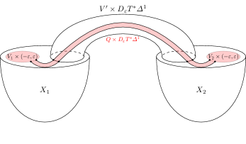
Figure 1. The Weinstein pair $(X_{1}\#_{V^{\prime}}X_{2},V_{1}\#_{Q}V_{2})$ obtained by gluing together the Weinstein pairs $(X_{1},W_{1})$ and $(X_{2},W_{2})$ along their common Weinstein subhypersurface $V^{\prime}\subset W_{1},W_{2}$.

1.3. Applications

A consequence of 1.1, and by known properties of the fully non-commutative knot contact homology for links, we obtain the following.

Theorem 1.5 (3.35).

Let $h$ be one of the two handle decompositions described in Section 3.4.1. Then $KCC^{\ast}(T,h)$ weakly detects the $1$-dimensional $r$-component untangle.

Remark 1.6.

The definition of weak detection is found in 3.34. The consequence of 1.1 is that $KCC^{\ast}(T,h)$ is a priori only able to detect tangles for which the isomorphism classes of the modules of oriented binormal geodesics between the tangle and $H$ are isomorphic to those corresponding to $T$. This seems like a rather mild restriction, see 3.36.

Knot contact homology of (framed oriented) knots in ${\mathbb{R}}^{3}$ is closely related to several smooth knot invariants. Some examples include string homology, the cord algebra, the Alexander polynomial and the augmentation polynomial which is closely related to the $A$-polynomial (and also conjectured to be related to a specialization of the HOMFLY-PT polynomial) [Ng05b, Ng08, CELN17, Ekh18]. The knot group and its peripheral subgroup can be extracted from the enhanced version of the knot contact homology [ENS18].

In view of 1.3, it is natural to propose the following conjecture, extending the scope of [CELN17, Theorem 1.1]. Roughly, we define $\operatorname{Cord}(T,H)$ to be the framed cord algebra of $T$, relative to $H$. In addition to the usual cord algebra of a tangle (which is defined by mimicking [Ng05b, Section 4.3] and [Ng08, Section 2.1]) we allow cords to have either or both endpoints on $H$.

Conjecture 1.7.

If $T$ is a framed oriented $r$-component tangle in ${\mathbb{R}}^{3}_{x\geq 0}$ there exists a choice of handle decomposition $h$ of $N(\varLambda_{T})$ such that we have an isomorphism of ${\mathbb{Z}}[\mu_{1}^{\pm 1},\ldots,\mu_{r}^{\pm 1}]$-algebras

$$KCH^{0}(T,h)\cong\operatorname{Cord}(T,H).$$

Remark 1.8.

We furthermore conjecture that the choice of handle decomposition in 1.7 should be such that there is a single top handle of $\varLambda_{T}$ (see Figure 16). There is a certain asymmetry in choices of handle decompositions $h_{1}$ and $h_{2}$ to recover $KCC^{\ast}_{\text{EENS}}(K)$ as described in Section 3.4.1. Thus we expect to find a gluing formula similar to that of 1.1, recovering $\operatorname{Cord}(K)$ from $\operatorname{Cord}(T_{1},H)$ and $\widetilde{\operatorname{Cord}}(T_{2},H)$ where $\widetilde{\operatorname{Cord}}(T_{2},H)\mathrel{\mathop{\mathchar 58\relax}}=KCH^{0}(T_{2},h_{2})$ with $h_{2}$ chosen as in Figure 15. We also expect there to be a suitable topological interpretation of $\widetilde{\operatorname{Cord}}(T_{2},H)$.

1.4. Related work

Dattin has defined a sutured Legendrian isotopy invariant of sutured Legendrian submanifolds in sutured contact manifolds called cylindrical sutured homology [Dat22]. In case the sutured contact manifold is balanced, we expect that the dg-algebra of $\varLambda_{T}\subset\partial T^{\ast}{\mathbb{R}}^{3}_{x\geq 0}$ defined by Dattin is quasi-isomorphic to $KCC^{\ast}(T,h)$.

Let $\varSigma$ be a surface without boundary and let $B\subset\varSigma\times[-1,1]$ be a braid. It is proven that a certain quotient of cylindrical sutured homology of $\varLambda_{B}\subset\partial T^{\ast}(\varSigma\times[-1,1])$ together with a product structure gives a complete invariant of braids [Dat22, Dat].

Outline

In Section 2 we generalize results from [Asp23]. Namely we construct simplicial decompositions of Weinstein pairs, and prove that the Chekanov–Eliashberg dg-algebra of top attaching spheres satisfies a gluing formula. This specializes to gluing formulas for the Chekanov–Eliashberg dg-algebra with loop space coefficients.

In Section 3 we define tangle contact homology for tangles in ${\mathbb{R}}^{3}_{x\geq 0}$. We apply the machinery of Section 2 to show that gluing of tangles induces gluing formulas for the tangle contact homologies.

In Section 4 we compute tangle contact homology in some examples and end with a calculation of the knot contact homology of the unknot via the gluing formula.

Acknowledgments

The author thanks Tobias Ekholm and Côme Dattin for helpful discussions, and Lenhard Ng for his correspondence. This paper grew out as an offshoot from on-going collaboration with William E. Olsen, to whom the author extends a special thanks to for carefully reading earlier drafts of this paper. The author was supported by the Knut and Alice Wallenberg Foundation.

2. Simplicial decompositions for Weinstein pairs

In this section we generalize the notion of a simplicial decomposition of a Weinstein manifold introduced in [Asp23] to Weinstein pairs.

2.1. Construction of simplicial decompositions for Weinstein pairs

We assume in the following that the reader is familiar with the construction of a simplicial decomposition of a Weinstein manifold as defined in [Asp23, Section 2.2].

Remark 2.1.

Recall that a Weinstein pair $(X^{2n},P^{2n-2})$ corresponds to a Weinstein sector $X^{\prime}$ via convex completion [GPS20, Section 2.7]. We may thus think about constructions in this section as a generalization of the simplicial decomposition of a Weinstein manifold as constructed in [Asp23] to a simplicial decomposition of a Weinstein sector.

In the following the superscript $X^{(k)}$ is used to indicate that $X$ has codimension $2k$ for $k\in{\mathbb{Z}}_{\geq 0}$. We give a quick recap of the definition of a simplicial decomposition and refer to [Asp23, Section 2.2] for details. A simplicial decomposition of a Weinstein manifold $X$ is a tuple $(C,\boldsymbol{V})$ where $C$ is a simplicial complex and $\boldsymbol{V}$ is a set containing one Weinstein manifold $V_{\sigma_{k}}^{(k)}$ for each $k$-face $\sigma_{k}\in C$ (ranging over all $k$) and a certain Weinstein hypersurface associated to each $k$-face $\sigma_{k}\in C$ (ranging over all $k$). Associated to each $V_{\sigma_{k}}^{(k)}$ is the “basic building block” $V_{\sigma_{k}}^{(k)}\times T^{\ast}\varDelta^{k}$ which is a Weinstein cobordism defined in [Asp23, Section 2.1]. We define $\#\boldsymbol{V}$ to be the gluing of all the building blocks $V_{\sigma_{k}}^{(k)}\times T^{\ast}\varDelta^{k}$ using certain gluing maps induced by the Weinstein hypersurfaces in $\boldsymbol{V}$. The condition required for $(C,\boldsymbol{V})$ to be a simplicial decomposition of $X$ is that there is a Weinstein isomorphism $X\cong\#\boldsymbol{V}$.

Definition 2.2.

Let $(C,\boldsymbol{V})$ be a simplicial decomposition. For a $k$-face $\sigma_{k}\in C$ we define $\boldsymbol{V}_{\supsetneq\sigma_{k}}\subset\boldsymbol{V}$ (and $\boldsymbol{V}_{\supset\sigma_{k}}\subset\boldsymbol{V}$) to be the subset consisting of only those Weinstein manifolds $V_{\sigma_{i}}\in\boldsymbol{V}$ for which $\sigma_{i}\supsetneq\sigma_{k}$ (and $\sigma_{i}\supset\sigma_{k}$), and the corresponding Weinstein hypersurfaces.

Definition 2.3 (Hypersurface inclusion of simplicial decompositions).

Let $(X,P)$ be a Weinstein pair. Let $(C,\boldsymbol{V})$ be a simplicial decomposition of $X^{2n}$ and let $(C^{\prime},\boldsymbol{V}^{\prime})$ be a simplicial decomposition of $P^{2n-2}$. A hypersurface inclusion of simplicial decompositions $(C^{\prime},\boldsymbol{V}^{\prime})\hookrightarrow(C,\boldsymbol{V})$ consists of

1. A simplicial subcomplex $i\colon C^{\prime}\hookrightarrow C$. When no confusion can arise we use the notation $\sigma_{k}\mathrel{\mathop{\mathchar 58\relax}}=i(\sigma^{\prime}_{k})$ for each $\sigma_{k}^{\prime}\in C^{\prime}$.

2. A Weinstein hypersurface

   $$\#(\boldsymbol{V}^{\prime}_{\supset\sigma_{k}^{\prime}}\sqcup_{i}\boldsymbol{V}_{\supsetneq\sigma_{k}})\hookrightarrow\partial V_{\sigma_{k}},$$

   for each $\sigma_{k}^{\prime}\in C^{\prime}$, where

   $$\boldsymbol{V}^{\prime}_{\supset\sigma_{k}^{\prime}}\sqcup_{i}\boldsymbol{V}_{\supsetneq\sigma_{k}}\mathrel{\mathop{\mathchar 58\relax}}=\boldsymbol{V}^{\prime}_{\supset\sigma_{k}^{\prime}}\cup\boldsymbol{V}_{\supsetneq\sigma_{k}}\cup\bigcup_{\sigma_{j}^{\prime}\supset\sigma_{k}^{\prime}}\{V^{\prime}_{\sigma_{j}^{\prime}}\hookrightarrow\partial V_{\sigma_{j}}\},$$

   see 2.2 and [Asp23, Section 2.2] for the notation.

Definition 2.4 (Simplicial decomposition of a Weinstein pair).

A simplicial decomposition of the Weinstein pair $(X,P)$ which is denoted by $((C,C^{\prime}),(\boldsymbol{V},\boldsymbol{V}^{\prime}))$ consists of

• A simplicial decomposition $(C,\boldsymbol{V})$ of $X$.

• A simplicial decomposition $(C^{\prime},\boldsymbol{V}^{\prime})$ of $P$.

• A hypersurface inclusion of simplicial decompositions $(C^{\prime},\boldsymbol{V}^{\prime})\hookrightarrow(C,\boldsymbol{V})$.

such that

$$X\cong\#\boldsymbol{V},\quad P\cong\#\boldsymbol{V}^{\prime}.$$

We now describe simplicial decompositions of Weinstein pairs in simple examples.

$C=\varDelta^{1}$:

A simplicial decomposition of $X$ over the $1$-simplex is a tuple $(\varDelta^{1},\boldsymbol{V})$ where $\boldsymbol{V}\mathrel{\mathop{\mathchar 58\relax}}=\left\{V^{2n-2},X^{2n}_{1},X^{2n}_{2},\iota_{1}\colon V\hookrightarrow\partial X_{1},\iota_{2}\colon V\hookrightarrow\partial X_{2}\right\}$. Here $V$ is a Weinstein $(2n-2)$-manifold corresponding to the single edge of $\varDelta^{1}$, $X_{1}^{2n}$ and $X_{2}^{2n}$ are two Weinstein $2n$-manifolds corresponding to each vertex of $\varDelta^{1}$ and $\iota_{1},\iota_{2}$ are two Weinstein hypersurfaces corresponding to the face inclusion of each vertex in the single edge of the $1$-simplex.

Using the tuple $(\varDelta^{1},\boldsymbol{V})$ we construct a Weinstein pair through the following surgery presentation. The basic building block associated to $V$ is the Weinstein cobordism $(V\times D_{\varepsilon}T^{\ast}\varDelta^{1},\lambda_{V}+2xdy+ydx)$ where $D_{\varepsilon}T^{\ast}\varDelta^{1}$ is the $\varepsilon$-disk cotangent bundle of $\varDelta^{1}$, $y$ is a coordinate in the $\varDelta^{1}$-factor and $x$ is a coordinate in the fiber direction. The negative end of this cobordism is $V\times D_{\varepsilon}T^{\ast}(\mathinner{\varDelta^{1}\rvert}_{\partial\varDelta^{1}})=(V\times(-\varepsilon,\varepsilon))\sqcup(V\times(-\varepsilon,\varepsilon))$. Using the Weinstein hypersurfaces $\iota_{1},\iota_{2}\in\boldsymbol{V}$ we attach the Weinstein cobordism $V\times D_{\varepsilon}T^{\ast}\varDelta^{1}$ to $X_{1}\sqcup X_{2}$ along $(V\times(-\varepsilon,\varepsilon))\sqcup(V\times(-\varepsilon,\varepsilon))$ and denote the resulting Weinstein manifold by $\#\boldsymbol{V}$, or $X_{1}\#_{V}X_{2}$ using more common notation, as this is nothing but the Weinstein connected sum of $X_{1}$ and $X_{2}$ over $V$ [Avd21, ÁGEN22, Eli18].

We require $C^{\prime}$ to be a simplicial subcomplex of $C$ and consider the two cases $C^{\prime}=\varDelta^{0},\varDelta^{1}$.

$C^{\prime}=\varDelta^{0}$:

In this case we set $\boldsymbol{V}^{\prime}=\left\{P^{2n-2}\right\}$. By 2.3 we now specify a hypersurface inclusion $(\varDelta^{0},\boldsymbol{V}^{\prime})\hookrightarrow(\varDelta^{1},\boldsymbol{V})$. It consists of an inclusion $\varDelta^{0}\hookrightarrow\varDelta^{1}$ as a simplicial subcomplex. We include $\varDelta^{0}$ into the first vertex, which corresponds to $X_{1}$. Next, we have a Weinstein hypersurface $\iota_{P,1}\colon P^{2n-2}\hookrightarrow\partial X^{2n}_{1}$ whose image is disjoint from the image of $\iota_{1}\in\boldsymbol{V}$. Item (3) is in fact equivalent to the data provided by item (2), because $\boldsymbol{V}_{\supsetneq\sigma_{0}}=\varnothing$ in this case, where $\sigma_{0}$ is the vertex of $C$ corresponding to $C^{\prime}$. Such a hypersurface inclusion $(\varDelta^{0},\boldsymbol{V}^{\prime})\hookrightarrow(\varDelta^{1},\boldsymbol{V})$ now allows us to construct the Weinstein pair $(X_{1}\#_{V}X_{2},P)$, by simply taking the Weinstein connected sum of $X_{1}$ and $X_{2}$ along $V$. The Weinstein hypersurface $P$ being disjoint from $V$ in $\partial X_{1}$ ensures that $P$ is a Weinstein hypersurface in $X_{1}\#_{V}X_{2}$, see Figure 2.

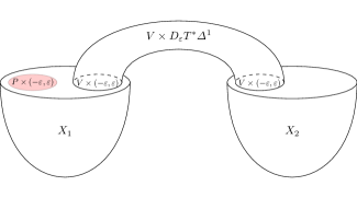
Figure 2. Left: The surgery presentation of the Weinstein pair $(X_{1}\#_{V}X_{2},P)$. Right: The simplicial subcomplex $C^{\prime}\hookrightarrow C$.

$C^{\prime}=\varDelta^{1}$:

In this case $\boldsymbol{V}^{\prime}=\left\{Q^{2n-4},P_{1}^{2n-2},P_{2}^{2n-2},\iota_{Q,1}\colon Q\hookrightarrow\partial P_{1}^{2n-2},\iota_{Q,2}\colon Q\hookrightarrow\partial P_{2}^{2n-2}\right\}$ where $Q$ is a Weinstein $(2n-4)$-manifold, $P_{1}$ and $P_{2}$ are Weinstein $(2n-2)$-manifolds and $\iota_{Q,1}$ and $\iota_{Q,2}$ are Weinstein hypersurfaces. This gives the surgery presentation $P=P_{1}\#_{Q}P_{2}$ as described above.

Pick the hypersurface inclusion $(\varDelta^{1},\boldsymbol{V}^{\prime})\hookrightarrow(\varDelta^{1},\boldsymbol{V})$ such that $\varDelta^{1}\hookrightarrow\varDelta^{1}$ is the identity map. By the definition 2.3 the hypersurface inclusion additionally consists of the following.

1. A Weinstein hypersurface $Q^{2n-4}\hookrightarrow\partial V^{2n-2}$.

2. Two Weinstein hypersurfaces $P_{i}\#_{Q}V\hookrightarrow\partial X_{i}$ for $i\in\left\{1,2\right\}$.

The Weinstein hypersurface $Q\hookrightarrow\partial V$ extends to a Weinstein hypersurface $Q\times D_{\varepsilon}T^{\ast}\varDelta^{1}\hookrightarrow\partial_{\infty}(V\times D_{\varepsilon}T^{\ast}\varDelta^{1})$ which is glued together with each of the negative ends of $Q\times D_{\varepsilon}T^{\ast}\varDelta^{1}\hookrightarrow\partial X_{i}$ along $\partial V$ for $i\in\left\{1,2\right\}$. The result is a Weinstein hypersurface $P_{1}\#_{Q}P_{2}\hookrightarrow\partial(X_{1}\#_{V}X_{2})$, see Figure 3.

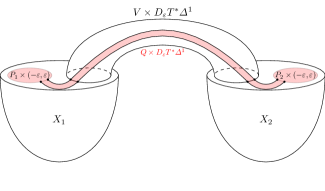
Figure 3. Left: The surgery presentation of the Weinstein pair $(X_{1}\#_{V}X_{2},\color[rgb]{1,0,0}{P_{1}\#_{Q}P_{2}}\color[rgb]{0,0,0}$. Right: The simplicial subcomplex $C^{\prime}\hookrightarrow C$.

$C=\varDelta^{2}$:

We consider a simplicial decomposition $(\varDelta^{2},\boldsymbol{V})$ of $X$ as follows. Let

$$\boldsymbol{V}\mathrel{\mathop{\mathchar 58\relax}}=\{V^{2n-2}_{1},V^{2n-2}_{2},V^{2n-2}_{3},W^{2n-4},X^{2n}_{1},X^{2n}_{2},X^{2n}_{3},\iota_{12},\iota_{23},\iota_{13},\iota_{1},\iota_{2},\iota_{3}\},$$

where

• $X_{1}$, $X_{2}$ and $X_{3}$ are Weinstein $2n$-manifolds corresponding to the vertices of $\varDelta^{2}$.

• $V_{1}$, $V_{2}$ and $V_{3}$ are Weinstein $(2n-2)$-manifolds corresponding to the edges of $\varDelta^{2}$.

• $W$ is a Weinstein $(2n-4)$-manifold corresponding to the $2$-face of $\varDelta^{2}$.

• $\iota_{i}\colon W\hookrightarrow\partial V_{i}$ is a Weinstein hypersurface for $i\in\left\{1,2,3\right\}$ corresponding to the inclusions of the edges into the $2$-simplex.

• $\iota_{12}\colon V_{1}\#_{W}V_{2}\hookrightarrow\partial X_{3}$, $\iota_{23}\colon V_{2}\#_{W}V_{3}\hookrightarrow\partial X_{1}$ and $\iota_{13}\colon V_{3}\#_{W}V_{1}\hookrightarrow\partial X_{2}$ are Weinstein hypersurfaces corresponding to the inclusion of the vertices into the $2$-simplex.

We describe a simplicial decomposition of the Weinstein pair $(X,P)$ in the two cases $C^{\prime}=\varDelta^{1}$ and $C^{\prime}=\varDelta^{2}$ below.

$C^{\prime}=\varDelta^{1}$:

As above we have a simplicial decomposition over the $1$-simplex $(\varDelta^{1},\boldsymbol{V}^{\prime})$ of $P$ so that $P\cong P_{1}\#_{Q}P_{2}$. We choose the hypersurface inclusion $(\varDelta^{1},\boldsymbol{V}^{\prime})\hookrightarrow(\varDelta^{2},\boldsymbol{V})$ that is given by the following.

1. An inclusion $\varDelta^{1}$ as a simplicial subcomplex of $\varDelta^{2}$ as the edge corresponding to $V_{1}$.

2. A Weinstein hypersurface $Q^{2n-4}\hookrightarrow\partial V_{1}^{2n-2}$.

3. Two Weinstein hypersurfaces $P_{1}\#_{Q}V_{1}\hookrightarrow\partial X_{2}$ and $P_{2}\#_{Q}V_{1}\hookrightarrow\partial X_{3}$.

As before the Weinstein hypersurface $Q\hookrightarrow\partial V$ extends to a Weinstein hypersurface $Q\times D_{\varepsilon}T^{\ast}\varDelta^{1}\hookrightarrow\partial_{\infty}(V\times D_{\varepsilon}T^{\ast}\varDelta^{1})$ which results in a Weinstein hypersurface $P_{1}\#_{Q}P_{2}\hookrightarrow\partial X$, see Figure 4

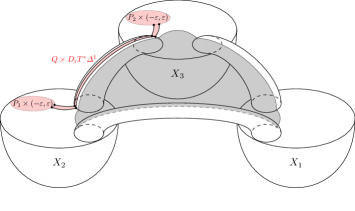
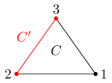
Figure 4. Left: The surgery presentation of the Weinstein pair $(\#\boldsymbol{V},P_{1}\#_{Q}P_{2})$. Right: The simplicial subcomplex ${\color[rgb]{1,0,0}{C^{\prime}}}\hookrightarrow C$ included as the edge in $C=\varDelta^{2}$ connecting the vertices $2$ and $3$.

$C^{\prime}=\varDelta^{2}$:

Pick a simplicial decomposition $(\varDelta^{2},\boldsymbol{V}^{\prime})$ of $P$ as follows. Let

$$\boldsymbol{V}^{\prime}\mathrel{\mathop{\mathchar 58\relax}}=\left\{Q_{1}^{2n-4},Q_{2}^{2n-4},Q_{3}^{2n-4},R^{2n-6},P^{2n-2}_{1},P^{2n-2}_{2},P^{2n-2}_{3},j_{12},j_{23},j_{13},j_{1},j_{2},j_{3}\right\},$$

where

• $P_{1}$, $P_{2}$ and $P_{3}$ are Weinstein $(2n-2)$-manifolds corresponding to the vertices of $\varDelta^{2}$.

• $Q_{1}$, $Q_{2}$ and $Q_{3}$ are Weinstein $(2n-4)$-manifolds corresponding to the edges of $\varDelta^{2}$.

• $R$ is a Weinstein $(2n-6)$-manifold corresponding to the $2$-face of $\varDelta^{2}$.

• $j_{i}\colon R\hookrightarrow\partial Q_{i}$ is a Weinstein hypersurface for $i\in\left\{1,2,3\right\}$ corresponding to the inclusions of the edges into the $2$-simplex.

• $j_{12}\colon Q_{1}\#_{R}Q_{2}\hookrightarrow\partial P_{3}$, $j_{23}\colon Q_{2}\#_{R}Q_{3}\hookrightarrow\partial P_{1}$ and $j_{13}\colon Q_{3}\#_{R}Q_{1}\hookrightarrow\partial P_{2}$ are Weinstein hypersurfaces corresponding to the inclusion of the vertices into the $2$-simplex.

We choose the hypersurface inclusion $(\varDelta^{2},\boldsymbol{V}^{\prime})\hookrightarrow(\varDelta^{2},\boldsymbol{V})$ that is given by the following.

1. The identity map $\varDelta^{2}\hookrightarrow\varDelta^{2}$.

2. Weinstein hypersurfaces $Q_{i}\hookrightarrow\partial V_{i}$ for $i\in\left\{1,2,3\right\}$ whose images are disjoint from the images of $\iota_{i}\in\boldsymbol{V}$.

3. A Weinstein hypersurface $\iota_{R}\colon R\hookrightarrow\partial W$.

4. Weinstein hypersurfaces $\iota_{i,R}\colon Q_{i}\#_{R}W\hookrightarrow\partial V_{i}$ for $i\in\left\{1,2,3\right\}$.

5. Weinstein hypersurfaces $\#\widetilde{\boldsymbol{V}}_{i}\hookrightarrow\partial X_{i}$ for $i\in\left\{1,2,3\right\}$ where

   $$\widetilde{\boldsymbol{V}}_{i} \mathrel{\mathop{\mathchar 58\relax}}=\left\{P_{i},R,W,\iota_{R}\right\}$$

   $$\qquad\cup\left\{Q_{k},V_{k},j_{k},\iota_{k,R}\right\}_{k\in\left\{1,2,3\right\}\setminus\left\{i\right\}}\cup\left\{j_{k\ell}\right\}_{\left\{k,\ell\right\}=\left\{1,2,3\right\}\setminus\left\{i\right\}}$$

   see Figure 5.

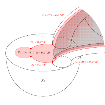
Figure 5. Part of the Weinstein hypersurface $P=\#\boldsymbol{V}^{\prime}$ lying in $\partial X_{2}$.

Each Weinstein hypersurface $\iota_{k,R}$ extends over the $1$-simplex handles $V_{k}\times D_{\varepsilon}T^{\ast}\varDelta^{1}$ to a Weinstein hypersurface

$$(Q_{k}\#_{R}W)\times D_{\varepsilon}T^{\ast}\varDelta^{1}\hookrightarrow\partial_{\infty}(V_{k}\times D_{\varepsilon}T^{\ast}\varDelta^{1}),$$

and the Weinstein hypersurface $\iota_{R}\colon R\hookrightarrow\partial W$ extends to a Weinstein hypersurface $R\times D_{\varepsilon}T^{\ast}\varDelta^{2}\hookrightarrow\partial_{\infty}(W\times D_{\varepsilon}T^{\ast}\varDelta^{2})$. These Weinstein hypersurfaces all glue together the same way as $2$-simplex handles are defined, see [Asp23, Section 2.2]. The result is a Weinstein hypersurface $\#\boldsymbol{V}^{\prime}\hookrightarrow\partial\left(\#\boldsymbol{V}\right)$, see Figure 6.

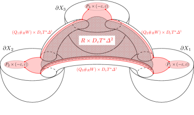
Figure 6. The Weinstein hypersurface $\#\boldsymbol{V}^{\prime}\hookrightarrow\partial\#\boldsymbol{V}$ depicted in red.

Remark 2.5.

From the point of view of Weinstein sectors, part of the the surgery description presented above corresponds to partial gluing of two Weinstein sectors along a shared subsector in the boundary, which was already described in [GPS22, Construction 12.18].

2.1.1. Good sectorial covers for sectors

The notion of a good sectorial cover of a Weinstein manifold introduced in [Asp23] now has a natural extension to Weinstein sectors. First recall the definition of a sectorial cover of a Liouville sector.

Definition 2.6 (Sectorial cover [GPS22, Definition 12.2 and Definition 12.19]).

Let $X$ be a Liouville sector. Suppose $X=X_{1}\cup\cdots\cup X_{n}$, where each $X_{i}$ is a manifold-with-corners with precisely two faces $\partial^{1}X_{i}\mathrel{\mathop{\mathchar 58\relax}}=X_{i}\cap\partial X$ and the point set topological boundary $\partial^{2}X_{i}$ of $X_{i}\subset X$, meeting along the corner locus $\partial X\cap\partial^{2}X_{i}=\partial^{1}X_{i}\cap\partial^{2}X_{i}$. Such a covering $X=X_{1}\cup\cdots\cup X_{n}$ is called sectorial if and only if $\forall i\in\left\{1,\ldots,n\right\}$ there are functions $I_{i}\colon N^{Z}(\partial^{2}X_{i})\longrightarrow{\mathbb{R}}$ (where $N^{Z}$ denotes a neighborhood which is cylindrical with respect to the Liouville vector field $Z$) which is linear at infinity such that:

• $X_{I_{i}}$ is outward pointing along $\partial^{2}X_{i}$.

• $X_{I_{i}}$ is tangent to $\partial^{2}X_{j}$ along $\partial^{2}X_{i}\cap\partial^{2}X_{j}$ for $i\neq j$.

• $[X_{I_{i}},X_{I_{j}}]=0$ along $N^{Z}(\partial^{2}X_{i})\cap N^{Z}(\partial^{2}X_{j})$.

Lemma 2.7 ([GPS22, Lemma 12.11]).

Let $X$ be a Liouville sector and suppose $X=X_{1}\cup\cdots\cup X_{n}$ is a sectorial cover. For any $\varnothing\neq A\subset\left\{1,\ldots,n\right\}$ we have a Liouville isomorphism

(2.1) $$N^{Z}\left(\bigcap_{i\in A}\partial^{2}X_{i}\right)\cong(X_{A}^{(k)}\times T^{\ast}{\mathbb{R}}^{k},\lambda_{X_{A}^{(k)}}+\lambda_{T^{\ast}{\mathbb{R}}^{k}}+df),$$

where $k\mathrel{\mathop{\mathchar 58\relax}}=\mathinner{\!\left\lvert A\right\rvert}-1$, $X^{(k)}_{A}$ is a $(2n-2k)$-dimensional Weinstein manifold and $f$ is a real-valued function on $X^{(k)}_{A}\times T^{\ast}{\mathbb{R}}^{k}$ with support in $K\times T^{\ast}{\mathbb{R}}^{k}$ for some compact $K\subset X^{(k)}_{A}$.

Definition 2.8 (Good sectorial cover).

Let $X$ be a Weinstein sector, and suppose $X=X_{1}\cup\cdots\cup X_{m}$ is a sectorial cover. We say that the sectorial cover is good if for every $\varnothing\neq A\subset\{1,\ldots,m\}$ we have a Weinstein isomorphism

(2.2) $$N^{Z}\left(\bigcap_{i\in A}X_{i}\right)\cong(X^{(k)}_{A}\times T^{\ast}{\mathbb{R}}^{k},\lambda_{X^{(k)}_{A}}+\lambda_{T^{\ast}{\mathbb{R}}^{k}}+df),$$

extending the Weinstein isomorphism (2.1), where $k\mathrel{\mathop{\mathchar 58\relax}}=\mathinner{\!\left\lvert A\right\rvert}-1$, $X^{(k)}_{A}$ is a $(2n-2k)$-dimensional Weinstein sector and $f$ is a real-valued function on $X^{(k)}_{A}\times T^{\ast}{\mathbb{R}}^{k}$ with support in $K\times T^{\ast}{\mathbb{R}}^{k}$ for some compact $K\subset X^{(k)}_{A}$.

Definition 2.9 (Simplicial decomposition of a Weinstein sector).

A simplicial decomposition of a Weinstein sector $X$ is defined to be a simplicial decomposition of the Weinstein pair $(\widetilde{X},P)$ which corresponds to $X$ via convex completion.

Theorem 2.10.

Let $X$ be a Weinstein sector. There is a one-to-one correspondence (up to Weinstein homotopy) between good sectorial covers of $X$ and simplicial decompositions of $X$.

Proof.

This is similar and a slight generalization of [Asp23, Theorem 3.11].

Given a simplicial decomposition $((C,C^{\prime}),(\boldsymbol{V},\boldsymbol{V}^{\prime}))$ of the Weinstein pair $(\widetilde{X},P)$, it follows from [Asp23, Theorem 3.11] that we obtain a good sectorial cover $\widetilde{X}=\widetilde{X}_{1}\cup\cdots\cup\widetilde{X}_{m}$ of $\widetilde{X}$. By definition we have that for any $\varnothing\neq A\subset\left\{1,\ldots,m\right\}$

$$N^{Z}\left(\bigcap_{i\in A}\widetilde{X}_{i}\right)\cong X_{A}^{(k)}\times T^{\ast}{\mathbb{R}}^{k},$$

where each $X_{A}^{(k)}$ is a Weinstein $(2n-2k)$-manifold. Letting $P_{A}\mathrel{\mathop{\mathchar 58\relax}}=\mathinner{P\rvert}_{A}$ with the restricted Weinstein structure gives a Weinstein manifold $P_{A}\hookrightarrow\partial X_{A}^{(k)}\times T^{\ast}{\mathbb{R}}^{k}$ which comes from a Weinstein hypersurface $P_{A}^{\prime}\hookrightarrow\partial X_{A}^{(k)}$. Each pair $(X_{A}^{(k)},P_{A}^{\prime})$ corresponds to a Weinstein $(2n-2k)$-sector $X_{A}^{(k)^{\prime}}$ via convex completion [GPS20, Section 2.7], and thus $\widetilde{X}_{1}\cup\cdots\cup\widetilde{X}_{m}$ is a good sectorial cover of $(\widetilde{X},P)$, which by definition is a good sectorial cover for $X$.

To finish the proof we need to reconstruct the simplicial decomposition $((C,C^{\prime}),(\boldsymbol{V},\boldsymbol{V}^{\prime}))$ of $(\widetilde{X},P)$ using the good sectorial cover $X_{1}\cup\cdots\cup X_{m}$ of $X$. For any $\varnothing\neq A\subset\left\{1,\ldots,m\right\}$ we have

$$N^{Z}\left(\bigcap_{i\in A}X_{i}\right)\cong X_{A}^{(k)}\times T^{\ast}{\mathbb{R}}^{k},$$

where each $X_{A}^{(k)}$ is a Weinstein $(2n-2k)$-sector which via convex completion [GPS20, Section 2.7] corresponds to the Weinstein pair $(X_{A}^{(k)^{\prime}},P_{A}^{\prime})$. The simplicial complex $C$ is given by the Čech nerve of the cover $X_{1}\cup\cdots\cup X_{m}$ of $X$. The simplicial subcomplex $i\colon C^{\prime}\hookrightarrow C$ is given by the Čech nerve of the restriction of the cover $X_{1}\cup\cdots\cup X_{m}$ to $\partial X$. The Weinstein hypersurface $P_{A}^{\prime}$ is precisely of the form $\#(\boldsymbol{V}^{\prime}_{\supset\sigma_{k}^{\prime}}\sqcup_{i}\boldsymbol{V}_{\supsetneq\sigma_{k}})\hookrightarrow\partial X_{A}^{(k)^{\prime}}$ where $\sigma_{k}$ is the face corresponding to $A\subset\left\{1,\ldots,m\right\}$. Forgetting the Weinstein hypersurface $P$ makes $X_{1}\cup\cdots\cup X_{m}$ a good sectorial cover of $\widetilde{X}$ which via [Asp23, Theorem 3.11] corresponds to a simplicial decomposition $(C,\boldsymbol{V})$. The set $\boldsymbol{V}^{\prime}_{\supset\sigma_{k}^{\prime}}$ consists of the Weinstein manifolds which are restrictions of $P_{A}^{\prime}$ to further intersections, with the corresponding Weinstein hypersurfaces which also is equal to a restriction of $P\hookrightarrow\partial\widetilde{X}$. Taking the union over all $\varnothing\neq A\subset\left\{1,\ldots,m\right\}$ we obtain $(C^{\prime},\boldsymbol{V}^{\prime})$ which by construction is a simplicial decomposition of $P$, and by construction we have a hypersurface inclusion $(C^{\prime},\boldsymbol{V}^{\prime})\hookrightarrow(C,\boldsymbol{V})$. ∎

2.2. Weinstein hypersurfaces and simplicial decompositions

We now review the definition of the Chekanov–Eliashberg dg-algebra of a Weinstein hypersurface with a chosen handle decomposition from [AE22] and review its relationship to Chekanov–Eliashberg dg-algebras with loop space coefficients. We describe the Chekanov–Eliashberg dg-algebra of a Weinstein hypersurface with respect to a simplicial decomposition of the corresponding Weinstein pair.

Let $X$ be a Weinstein $2n$-manifold and let $V^{2n-2}\hookrightarrow\partial X^{2n}$ be a Weinstein hypersurface. Fix a Weinstein handle decomposition $h$ of $V$ which encodes both the Weinstein handles and the attaching maps. Now let $X_{V}$ be the Weinstein cobordism obtained by attaching the $1$-simplex handle $V\times D_{\varepsilon}T^{\ast}\varDelta^{1}$ to $X\sqcup({\mathbb{R}}\times(V\times{\mathbb{R}}))$, and let $\varSigma(h)$ denote the union of attaching spheres of the top handles of $V\times D_{\varepsilon}T^{\ast}\varDelta^{1}$ in $X_{V}$. This is a link of Legendrian spheres in the positive end of $X_{V_{0}}$.

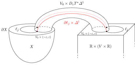
Figure 7. The Weinstein cobordism $X_{V}$ which we identify as the Weinstein manifold $X$ stopped at the Weinstein hypersurface $V\hookrightarrow\partial X$.

The union of Legendrian spheres $\varSigma(h)$ has the following geometric description.

Lemma 2.11.

Let $\ell\mathrel{\mathop{\mathchar 58\relax}}=\bigcup_{j}\ell_{j}$ denote the union of the core disks of the top handles in $h$. Then we have

$$\varSigma(h)=\ell\cup_{\partial\ell\times\left\{-1\right\}}(\partial\ell\times\varDelta^{1})\cup_{\partial\ell\times\left\{1\right\}}\ell.$$

Additionally let $\kappa\mathrel{\mathop{\mathchar 58\relax}}=\bigcup_{i}\kappa_{i}$ denote the union of attaching spheres of the top handles of $X$. Then $\varSigma(h)\cup\kappa$ is the union of attaching spheres of the top Weinstein handles of $X_{V}$.

Proof.

This is part of [AE22, Lemma 3.1], cf. [Asp23, Definition 2.20]. ∎

Lemma 2.12.

For all $\mathfrak{a}>0$ there exists some $\delta>0$ and an arbitrary small perturbation of $V_{0}$ such that for all $0<\varepsilon<\delta$ the Reeb chords of $\varSigma(h)$ of action $<\mathfrak{a}$ are in one-to-one grading preserving correspondence with Reeb chords of $\ell\subset\partial X_{0}$, and Reeb chords of $\partial\ell\subset\partial V_{0}$ of action $<\mathfrak{a}$.

Proof.

See [AE22, Lemma 2.3], cf. [Asp23, Lemma 2.24]. ∎

Definition 2.13 ([AE22, Definition 3.2]).

Let $X$ be a Weinstein manifold and $V\hookrightarrow\partial X$ a Weinstein hypersurface together with a chosen handle decomposition $h$ of $V$. We define the Chekanov–Eliashberg dg-algebra of the pair $(V,h)$ as

$$CE^{\ast}((V,h);X)\mathrel{\mathop{\mathchar 58\relax}}=CE^{\ast}(\varSigma(h);X_{V_{0}}).$$

Lemma 2.14 ([AE22, Corollary 2.11]).

There is a dg-subalgebra of $CE^{\ast}((V,h);X)$ which is canonically quasi-isomorphic to $CE^{\ast}(\partial\ell;V_{0})$.

Lemma 2.15 ([AE22, Lemma 4.2]).

Let $X$ be a Weinstein manifold and $\varLambda\subset\partial X$ a smooth Legendrian submanifold. Let $V$ be a small cotangent neighborhood of $\varLambda$ and let $h$ be a choice of handle decomposition of $V$ with a single top handle. There is a quasi-isomorphism of dg-algebras

$$CE^{\ast}(\partial\ell;V_{0})\cong C_{-\ast}(\varOmega\varLambda).$$

Proof.

The idea of the proof is to construct a map $\varphi\colon CE^{\ast}(\partial\ell;V_{0})\longrightarrow C_{-\ast}(\varOmega\varLambda)$ by counting $J$-holomorphic curves in $V_{0}$ such that the following diagram commutes up to dg-homotopy.

$$\leavevmode\hbox to122.54pt{\vbox to49.41pt{\text{[drawing]}}}. {CW^{\ast}(F,F)} {C_{-\ast}(\varOmega\varLambda)} {CE^{\ast}(\partial\ell;V_{0})} \scriptstyle{\varPsi} \scriptstyle{\varPhi} \scriptstyle{\varphi} {CW^{\ast}(F,F)} {C_{-\ast}(\varOmega\varLambda)} {CE^{\ast}(\partial\ell;V_{0})} \scriptstyle{\varPsi} \scriptstyle{\varPhi} \scriptstyle{\varphi}$$

Here $F$ denotes a cotangent fiber in the Weinstein neighborhood $T^{\ast}\varLambda$ of $\varLambda\subset\partial X$. The map $\varPsi$ is the surgery $A_{\infty}$-quasi-isomorphism from [BEE12], and $\varPhi$ is the $A_{\infty}$-quasi-isomorphism from [Abo12, Asp21], see [AE22, Section 4] for details. ∎

The following is now an immediate consequence of 2.15 and one of the main results of [AE22].

Theorem 2.16 ([AE22, Theorem 1.2]).

Let $X$ be a Weinstein manifold and $\varLambda\subset\partial X$ a smooth (possibly disconnected) Legendrian submanifold. Let $V$ be a small cotangent neighborhood of $\varLambda$ and let $h$ be a choice of handle decomposition such that $V$ has a single top handle for each component of $V$. There is a quasi-isomorphism of dg-algebras

$$CE^{\ast}((V,h);X)\cong CE^{\ast}\left(\varLambda,C_{-\ast}\left(\bigsqcup_{i\in\pi_{0}(\varLambda)}\varOmega\varLambda_{i}\right)\right),$$

where $\varLambda_{i}$ denotes the $i$-th component of $\varLambda$ and where $CE^{\ast}(\varLambda,C_{-\ast}(\varOmega\varLambda))$ is the Chekanov–Eliashberg dg-algebra with loop space coefficients as defined in [EL17].

Proof.

See [AE22, Section 4]. ∎

Let $(X,P)$ be a Weinstein pair and let $((C,C^{\prime}),(\boldsymbol{V},\boldsymbol{V}^{\prime}))$ be a simplicial decomposition of $(X,P)$. Pick a handle decomposition for each $V_{\sigma_{k}}\in\boldsymbol{V}$ and denote the set of all such by $\boldsymbol{h}$. Similarly let $\boldsymbol{h}^{\prime}$ denote the set of chosen handle decompositions of each $V_{\sigma_{k}^{\prime}}^{\prime}\in\boldsymbol{V}^{\prime}$. The union of the top attaching spheres of $X\cong\#\boldsymbol{V}$ is denoted by $\varSigma(\boldsymbol{h})$, see [Asp23, Definition 2.20 and Lemma 2.21] for details on the constructions.

Figure 8. The Weinstein hypersurface $P\hookrightarrow\partial X$ presented as a join with respect to the simplicial decomposition $((C,C^{\prime}),(\boldsymbol{V},\boldsymbol{V}^{\prime}),(\boldsymbol{A},\boldsymbol{A}^{\prime}))$ where $C=C^{\prime}=\varDelta^{2}$ and the simplicial subcomplex $C^{\prime}\hookrightarrow C$ being the identity map.

We now describe the union of the top attaching spheres of $X_{P}$ with respect to the simplicial decomposition of $(X,P)$. Let $\ell^{\prime}=\bigcup_{\sigma_{k}^{\prime}\in C^{\prime}}\ell^{\prime}_{\sigma_{k}^{\prime}}=\bigcup_{\sigma_{k}^{\prime}\in C^{\prime}}\bigcup_{j}\ell^{\prime}_{\sigma_{k}^{\prime},j}$ denote the union of the core disks of the top handles of each $V^{\prime}_{\sigma_{k}^{\prime}}\in\boldsymbol{V}^{\prime}$. Let $i\colon C^{\prime}\hookrightarrow C$ be the simplicial subcomplex in the simplicial decomposition of $(X,P)$. For every $\sigma_{0}\in\operatorname{im}i$ we have the Weinstein hypersurface

(2.3) $$\#(\boldsymbol{V}^{\prime}_{\supset\sigma_{0}^{\prime}}\sqcup_{i}\boldsymbol{V}_{\supsetneq\sigma_{0}})\hookrightarrow\partial V_{\sigma_{0}},$$

as in 2.3, see Figure 9.

Denote the union of the top attaching spheres of the $\#(\boldsymbol{V}^{\prime}_{\supset\sigma_{0}}\sqcup_{i}\boldsymbol{V}_{\supsetneq\sigma_{0}})$ by $\varSigma(\boldsymbol{h}^{\prime}_{\sigma_{0}^{\prime}}\sqcup_{i}\boldsymbol{h}_{\sigma_{0}})$ where $\boldsymbol{h}^{\prime}_{\sigma_{0}^{\prime}}\sqcup_{i}\boldsymbol{h}_{\sigma_{0}}$ is the union of handle decompositions of the Weinstein manifolds in $\boldsymbol{V}^{\prime}_{\supset\sigma_{0}}\sqcup_{i}\boldsymbol{V}_{\supsetneq\sigma_{0}}$. Let $\varDelta(\boldsymbol{h}^{\prime}_{\sigma_{0}^{\prime}}\sqcup_{i}\boldsymbol{h}_{\sigma_{0}})$ be the corresponding union of core disks of the top handles in $\boldsymbol{h}^{\prime}_{\sigma_{0}^{\prime}}\sqcup_{i}\boldsymbol{h}_{\sigma_{0}}$, and note that topologically $\varDelta(\boldsymbol{h}^{\prime}_{\sigma_{0}^{\prime}}\sqcup_{i}\boldsymbol{h}_{\sigma_{0}})$ is a union of $(n-1)$-disks in $\partial V_{\sigma_{0}}$ via the Weinstein embedding (2.3).

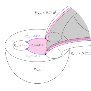
Figure 9. The Weinstein hypersurface $\#(\boldsymbol{V}^{\prime}_{\supset(\sigma_{0})_{2}}\sqcup_{i}\boldsymbol{V}_{\supsetneq(\sigma_{0})_{2}})\hookrightarrow\partial X_{(\sigma_{0})_{2}}$ which is a part of the construction of $P\hookrightarrow\partial X$ with respect to the simplicial decomposition $((C,C^{\prime}),(\boldsymbol{V},\boldsymbol{V}^{\prime}))$ as in Figure 8. The Weinstein hypersurfaces $V^{\prime}_{(\sigma_{1}^{\prime})_{3}}\#_{V^{\prime}_{\sigma_{2}^{\prime}}}W\hookrightarrow\partial V_{3}$ and $V^{\prime}_{(\sigma_{1}^{\prime})_{1}}\#_{V^{\prime}_{\sigma_{2}^{\prime}}}W\hookrightarrow\partial V_{1}$ are also depicted.

We then extend every $\varDelta(\boldsymbol{h}^{\prime}_{\sigma_{0}^{\prime}}\sqcup_{i}\boldsymbol{h}_{\sigma_{0}})$ trivially $\#\boldsymbol{V}\cong X$ and denote the result by $\varSigma_{P}(\boldsymbol{h}^{\prime})$. The result is the union of top attaching spheres of the Weinstein manifold $P\cong\#\boldsymbol{V}^{\prime}$, see [Asp23, Definition 2.20]. By construction we have a decomposition $\varSigma_{P}(\boldsymbol{h}^{\prime})=\bigcup_{\sigma_{k}^{\prime}\in C^{\prime}}\varSigma_{P,\sigma_{k}^{\prime}}(\boldsymbol{h}^{\prime})$, where $\varSigma_{P,\sigma_{k}^{\prime}}(\boldsymbol{h}^{\prime})$ is the union of the top attaching spheres of $P$ living over the locus corresponding to the $k$-face $\sigma_{k}^{\prime}\in C^{\prime}$.

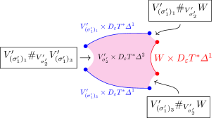
Figure 10. The first gluing step in the construction of the Weinstein hypersurface $\#(\boldsymbol{V}^{\prime}_{\supset(\sigma_{0})_{2}}\sqcup_{i}\boldsymbol{V}_{\supsetneq(\sigma_{0})_{2}})\hookrightarrow\partial X_{(\sigma_{0})_{2}}$ in Figure 9.

Lemma 2.17.

The union of $(n-1)$-spheres $\varSigma_{P}(\boldsymbol{h}^{\prime})$ is the union of the attaching spheres of the top handles of the Weinstein manifold $P$.

Proof.

This is repetition of the proof of [Asp23, Lemma 2.21]. ∎

Let $\varDelta_{P}(\boldsymbol{h}^{\prime})$ denote the union of the core disks of the top handles in $\boldsymbol{h}^{\prime}$. Since we have a Weinstein hypersurface $P\hookrightarrow\partial X$, it follows that $\varDelta_{P}(\boldsymbol{h}^{\prime})$ is a Legendrian submanifold in $\partial X$ with boundary in $\partial P$. Like the attaching spheres, the core disks also decompose as $\varDelta_{P}(\boldsymbol{h}^{\prime})=\bigcup_{\sigma_{k}^{\prime}\in C^{\prime}}\varDelta_{P,\sigma_{k}^{\prime}}(\boldsymbol{h}^{\prime})$ where $\varDelta_{P,\sigma_{k}^{\prime}}(\boldsymbol{h}^{\prime})$ is the core disk with boundary $\partial\varDelta_{P,\sigma_{k}^{\prime}}(\boldsymbol{h}^{\prime})=\varSigma_{P,\sigma_{k}^{\prime}}(\boldsymbol{h}^{\prime})$.

Our next task is to describe the Chekanov–Eliashberg dg-algebra of the pair $(P,\boldsymbol{h}^{\prime})$ in $X$. To that end, we construct $X_{P_{0}}$ by attaching the handle $P_{0}\times D_{\varepsilon}T^{\ast}\varDelta^{1}$ to $X\sqcup({\mathbb{R}}\times(P\times{\mathbb{R}}))$. By 2.11 we have that the union of attaching spheres of $X_{P_{0}}$ is

(2.4) $$\varSigma_{X_{P}}(\boldsymbol{h}^{\prime})\mathrel{\mathop{\mathchar 58\relax}}=\varDelta_{P}(\boldsymbol{h}^{\prime})\cup_{\partial\varDelta_{P}(\boldsymbol{h}^{\prime})\times\left\{-1\right\}}(\partial\varDelta_{P}(\boldsymbol{h}^{\prime})\times\varDelta^{1})\cup_{\partial\varDelta_{P}(\boldsymbol{h}^{\prime})\times\left\{1\right\}}\varDelta_{P}(\boldsymbol{h}^{\prime}).$$

Below a given action bound on Reeb chords, and for arbitrarily thin simplicial handles it follows from 2.12 that the Reeb chords of $\varSigma_{X_{P}}(\boldsymbol{h}^{\prime})$ corresponds to Reeb chords of $\varDelta_{P}(\boldsymbol{h}^{\prime})\subset\partial X_{0}$ and Reeb chords of $\partial\varDelta_{P}(\boldsymbol{h}^{\prime})=\varSigma_{P}(\boldsymbol{h}^{\prime})\subset\partial P_{0}$.

Definition 2.18 ([Asp23, Definition 2.22]).

Let $(C,\boldsymbol{V})$ be a simplicial decomposition of $X$ and let $\boldsymbol{h}$ be a choice of handle decomposition of $\boldsymbol{V}$. Denote the union of core disks of the top handles in $\boldsymbol{h}$ by $\ell$.

1. Let $\mathcal{R}_{X}(\sigma_{k})$ denote the set of Reeb chords of $\partial\ell_{\sigma_{k}}\cup\bigcup_{\begin{subarray}{c}\sigma_{i}\supset\sigma_{k}\\ k+1\leq i\leq m\end{subarray}}(\ell_{\sigma_{i}}\times\varDelta^{i-k-1})\subset\partial V^{(k)}_{\sigma_{k},0}$ for $k\in\left\{0,\ldots,m\right\}$, where $\ell_{\sigma_{i}}\times\varDelta^{i-k-1}$ are the core disks of the top handles of $V^{(i)}_{\sigma_{i},0}\times D_{\varepsilon}T^{\ast}\varDelta^{i-k-1}\hookrightarrow\partial V^{(k)}_{\sigma_{k},0}$.

2. Let $\mathcal{R}_{X}(\sigma_{k},\mathfrak{a})$ denote the set of Reeb chords in $\mathcal{R}_{X}(\sigma_{k})$ of action $<\mathfrak{a}$.

Definition 2.19.

Let $((C,C^{\prime}),(\boldsymbol{V},\boldsymbol{V}^{\prime}))$ be a simplicial decomposition of the Weinstein pair $(X,P)$. Let $\boldsymbol{h}$ and $\boldsymbol{h}^{\prime}$ be choices of handle decompositions of $\boldsymbol{V}$ and $\boldsymbol{V}^{\prime}$ respectively. Denote the union of core disks of the top handles in $\boldsymbol{h}$ and $\boldsymbol{h}^{\prime}$ by $\ell$ and $\ell^{\prime}$ respectively.

1. Let $\mathcal{R}_{(X,P)}(\sigma_{k}^{\prime})$ denote the set of Reeb chords of $\ell^{\prime}_{\sigma_{k}^{\prime}}\cup\bigcup_{\begin{subarray}{c}\sigma_{i}^{\prime}\supset\sigma_{k}^{\prime}\\ k+1\leq i\leq m^{\prime}\end{subarray}}(\ell^{\prime}_{\sigma_{i}^{\prime}}\times\varDelta^{i-k})$ for $k\in\left\{0,\ldots,m^{\prime}\right\}$, where $\ell^{\prime}_{\sigma_{i}^{\prime}}\times\varDelta^{i-k}$ are the core disks of the top handles of $V^{\prime(i)}_{\sigma_{i}^{\prime},0}\times D_{\varepsilon}T^{\ast}\varDelta^{i-k}\hookrightarrow\partial V_{\sigma_{k},0}^{(k)}$.

2. Let $\mathcal{R}_{(X,P)}(\sigma_{k}^{\prime},\mathfrak{a})$ denote the set of Reeb chords in $\mathcal{R}_{(X,P)}(\sigma_{k}^{\prime})$ of action $<\mathfrak{a}$.

Recall that the precise construction of $\#\boldsymbol{V}$ depends on a size parameter $\boldsymbol{\varepsilon}=\left\{0<\varepsilon_{m}<\cdots<\varepsilon_{1}\right\}$, where each $\varepsilon_{k}>0$ is the size of the simplicial handle $H^{k}_{\varepsilon_{k}}(V^{2n-2k}_{\sigma_{k}})$, see [Asp23, Definition 2.11]. For notational simplicity we write $0<\boldsymbol{\varepsilon}<\delta$ to mean $0<\varepsilon_{m}$ and $\varepsilon_{1}<\delta$.

Lemma 2.20.

For all $\mathfrak{a}>0$ there exists some $\delta>0$ and an arbitrary small perturbation of $\boldsymbol{V}_{0}$ such that for all $0<\boldsymbol{\varepsilon}<\delta$ the following holds.

1. There is a one-to-one grading preserving correspondence between Reeb chords of action $<\mathfrak{a}$ of $\varDelta_{P}(\boldsymbol{h}^{\prime})\subset\partial X_{0}$ and Reeb chords in $\bigcup_{\begin{subarray}{c}\sigma_{k}^{\prime}\in C^{\prime}\\ 0\leq k\leq m^{\prime}\end{subarray}}\mathcal{R}_{(X,P)}(\sigma_{k}^{\prime},\mathfrak{a})$.

2. There is a one-to-one grading preserving correspondence between Reeb chords of $\partial\varDelta_{P}(\boldsymbol{h}^{\prime})\subset\partial P_{0}$ of action $<\mathfrak{a}$ and Reeb chords in $\bigcup_{\begin{subarray}{c}\sigma_{k}^{\prime}\in C^{\prime}\\ 0\leq k\leq m^{\prime}\end{subarray}}\mathcal{R}_{P}(\sigma_{k}^{\prime},\mathfrak{a})$.

Proof.

1. It follows from the construction of $\#\boldsymbol{V}$ that Reeb chords of $\varDelta_{P}(\boldsymbol{h}^{\prime})\subset\partial X_{0}$ of action $<\mathfrak{a}$ (possibly after shrinking the size of the simplicial handles) are contained in $\pi^{-1}(0,0)$ where $\pi\colon\partial V^{(k)}_{\sigma_{k}}\times D_{\varepsilon}T^{\ast}\varDelta^{k}\longrightarrow D_{\varepsilon}T^{\ast}\varDelta^{k}$ is the projection to the second factor, corresponding to each $\sigma_{k}\in C$, see [Asp23, Lemma 2.24]. It follows from the construction of $\varDelta_{P}(\boldsymbol{h}^{\prime})$ that the part lying in the positive contact boundary of $V^{(k)}_{\sigma_{k}}\times D_{\varepsilon}T^{\ast}\varDelta^{k}$ has the form $(\ell^{\prime}_{\sigma_{k}^{\prime}}\times\varDelta^{k})\cup\bigcup_{\begin{subarray}{c}\sigma_{i}^{\prime}\supset\sigma_{k}^{\prime}\\ k+1\leq i\leq m^{\prime}\end{subarray}}(\ell^{\prime}_{\sigma_{i}^{\prime}}\times\varDelta^{i})$ from which the result follows.

2. The proof is the same as in (1) above.

∎

2.3. Simplicial descent for Weinstein pairs

Let $((C,C^{\prime}),(\boldsymbol{V},\boldsymbol{V}^{\prime}))$ be a simplicial decomposition of a Weinstein pair $(X,P)$. In this section we prove that we have a gluing formula for the Chekanov–Eliashberg dg-algebra $CE^{\ast}((P,\boldsymbol{h}^{\prime});X)$. In a special case this may be regarded as a gluing formula for the Chekanov–Eliashberg dg-algebra with loop space coefficients, see 2.24.

Let $\boldsymbol{h}$ and $\boldsymbol{h}^{\prime}$ be handle decompositions of $\boldsymbol{V}$ and $\boldsymbol{V}^{\prime}$ respectively, as in Section 2.2. Let $\varSigma_{X_{P}}(\boldsymbol{h}^{\prime})\subset\partial X_{P_{0}}$ be the union of the top attaching spheres of the simplicial handle $P_{0}\times D_{\varepsilon}T^{\ast}\varDelta^{1}$. We use the notation

$$\varDelta_{P,\supset\sigma_{k}^{\prime}}(\boldsymbol{h}^{\prime})\mathrel{\mathop{\mathchar 58\relax}}=\bigcup_{\begin{subarray}{c}\sigma_{i}^{\prime}\supset\sigma_{k}^{\prime}\\ k\leq i\leq m^{\prime}\end{subarray}}\varDelta_{P,\sigma_{i}^{\prime}}(\boldsymbol{h}^{\prime}),\quad\varSigma_{X_{P},\supset\sigma_{k}^{\prime}}(\boldsymbol{h}^{\prime})\mathrel{\mathop{\mathchar 58\relax}}=\bigcup_{\begin{subarray}{c}\sigma_{i}^{\prime}\supset\sigma_{k}^{\prime}\\ k\leq i\leq m^{\prime}\end{subarray}}\varSigma_{X_{P},\sigma_{i}^{\prime}}(\boldsymbol{h}^{\prime}).$$

From [Asp23, Section 2.5.1] we recall the following. For each $k$-face $\sigma_{k}\in C$ define

(2.5) $$\widetilde{V}^{(i)}_{\sigma_{i}}(\sigma_{k})\mathrel{\mathop{\mathchar 58\relax}}=\begin{cases}V^{(i)}_{\sigma_{i}}&\text{if }\sigma_{i}\supset\sigma_{k}\\ (-\infty,0]\times\bigsqcup_{f\in F}(\#\widetilde{\boldsymbol{V}}_{\supsetneq\sigma_{i},f}(\sigma_{k}))\times{\mathbb{R}}&\text{otherwise}\end{cases}$$

where $\widetilde{\boldsymbol{V}}_{\supsetneq\sigma_{i},f}(\sigma_{k})$ is the set of Weinstein manifolds $\widetilde{V}^{(\ell)}_{\sigma_{\ell}}(\sigma_{k})$ for $f\supset\sigma_{\ell}\supsetneq\sigma_{i}$ with the same Weinstein hypersurfaces as in $\boldsymbol{V}$, and the Weinstein hypersurfaces induced by the inclusion $\{0\}\times(W\times\left\{0\right\})\hookrightarrow(-\infty,0]\times(W\times{\mathbb{R}})$ for those $\widetilde{V}^{(\ell)}_{\sigma_{\ell}}(\sigma_{k})$ of the form as in the bottom row of (2.5). Finally define $\widetilde{\boldsymbol{V}}(\sigma_{k})\mathrel{\mathop{\mathchar 58\relax}}=\bigcup_{\begin{subarray}{c}f\in F\\ \sigma_{i}\subset f\end{subarray}}\widetilde{\boldsymbol{V}}_{\supsetneq\sigma_{i},f}(\sigma_{k})$ and

(2.6) $$X(\sigma_{k})\mathrel{\mathop{\mathchar 58\relax}}=\#\widetilde{\boldsymbol{V}}(\sigma_{k})\,.$$

Similarly, for each $\sigma_{k}\in C$ we define the Weinstein hypersurface $P(\sigma_{k})\hookrightarrow\partial X(\sigma_{k})$ as follows. If $\sigma_{k}\not\in\operatorname{im}i$, then $P(\sigma_{k})\mathrel{\mathop{\mathchar 58\relax}}=P$. Else $P(\sigma_{k}^{\prime})$ is defined in analogy with $X(\sigma_{k})$ above.

Lemma 2.21.

For all $\mathfrak{a}>0$ there exists some $\delta>0$ and an arbitrary small perturbation of $\boldsymbol{V}_{0}$ such that for all $0<\boldsymbol{\varepsilon}<\delta$ the following holds.

1. There is a one-to-one grading preserving correspondence between Reeb chords of action $<\mathfrak{a}$ of $\partial\varDelta_{P,\supset\sigma_{k}^{\prime}}(\boldsymbol{h}^{\prime})\subset\partial P(\sigma_{k}^{\prime})_{0}$ and Reeb chords in $\bigcup_{\sigma_{i}^{\prime}\supset\sigma_{k}^{\prime}}\mathcal{R}_{P}(\sigma_{i}^{\prime},\mathfrak{a})$.

2. There is a one-to-one grading preserving correspondence between Reeb chords of action $<\mathfrak{a}$ of $\varDelta_{P,\supset\sigma_{k}^{\prime}}(\boldsymbol{h}^{\prime})\subset\partial(X(\sigma_{k}^{\prime}))_{P(\sigma_{k}^{\prime})_{0}}$ and Reeb chords in $\bigcup_{\sigma_{i}^{\prime}\supset\sigma_{k}^{\prime}}\mathcal{R}_{(X,P)}(\sigma_{i}^{\prime},\mathfrak{a})$.

3. There is a one-to-one grading preserving correspondence between Reeb chords of action $<\mathfrak{a}$ of $\varSigma_{X_{P},\supset\sigma_{k}^{\prime}}(\boldsymbol{h}^{\prime})\subset\partial(X(\sigma_{k}^{\prime}))_{P(\sigma_{k}^{\prime})_{0}}$ and Reeb chords in $\bigcup_{\sigma_{i}^{\prime}\supset\sigma_{k}^{\prime}}(\mathcal{R}_{(X,P)}(\sigma_{i}^{\prime},\mathfrak{a})\cup\mathcal{R}_{P}(\sigma_{i}^{\prime},\mathfrak{a}))$.

Proof.

1. This follows from [Asp23, Lemma 2.36].

2. For sufficient thin handles, the Reeb chords in $\bigcup_{\sigma_{i}^{\prime}\supset\sigma_{k}^{\prime}}\mathcal{R}_{(X,P)}(\sigma_{i}^{\prime},\mathfrak{a})$ corresponds to Reeb chords of $\varDelta_{P,\supset\sigma_{k}^{\prime}}(\boldsymbol{h}^{\prime})\subset\partial X_{P_{0}}$ appearing in the loci of the contact boundary of $X_{P_{0}}$ corresponding to $\sigma_{i}^{\prime}\supset\sigma_{k}^{\prime}$ in the simplicial decomposition of $X$ in as in the proof of 2.20. These loci in $X_{P_{0}}$ are precisely those that are unchanged in the definition of $\widetilde{\boldsymbol{V}}(\sigma_{k}^{\prime})$, see (2.5). The previously existing Reeb chords of $\varDelta_{P,\supset\sigma_{k}^{\prime}}(\boldsymbol{h}^{\prime})\subset\partial X_{P_{0}}$ lying over critical points in loci corresponding to $i$-faces $\sigma_{i}^{\prime}\not\supset\sigma_{k}^{\prime}$ disappear when passing to $\partial(X(\sigma_{k}^{\prime}))_{P(\sigma_{k}^{\prime})_{0}}$, as the contact manifold in these loci are of the form $W\times{\mathbb{R}}$, where the Legendrian is contained in the ${\mathbb{R}}$-factor, see (2.5).

3. By construction of $\varSigma_{X_{P},\supset\sigma_{k}^{\prime}}(\boldsymbol{h}^{\prime})$, see (2.4), this follows from items (1) and (2).

∎

Theorem 2.22.

1. There is a quasi-isomorphism of dg-algebras

   $$CE^{\ast}(\partial\varDelta_{P}(\boldsymbol{h}^{\prime});P_{0})\cong\operatorname*{colim}_{\sigma_{k}^{\prime}\in C^{\prime}}CE^{\ast}(\partial\varDelta_{P,\supset\sigma_{k}^{\prime}};P(\sigma_{k}^{\prime})_{0}).$$

2. There is a quasi-isomorphism of dg-algebras

   $$CE^{\ast}(\varSigma_{X_{P}}(\boldsymbol{h}^{\prime});(X_{P})_{0})\cong\operatorname*{colim}_{\sigma_{k}^{\prime}\in C^{\prime}}CE^{\ast}(\varSigma_{X_{P},\supset\sigma_{k}^{\prime}}(\boldsymbol{h}^{\prime});X(\sigma_{k}^{\prime})_{P(\sigma_{k}^{\prime})_{0}}).$$

Proof.

Let $\delta,\mathfrak{a}>0$ and $0<\boldsymbol{\varepsilon}<\delta$.

1. For any $\sigma_{k}^{\prime}\in C^{\prime}$, define $\mathcal{A}_{P,\sigma_{k}^{\prime}}(\boldsymbol{h}^{\prime};\boldsymbol{\varepsilon},\mathfrak{a})$ to be the dg-algebra generated by Reeb chords in $\bigcup_{\sigma_{i}^{\prime}\supset\sigma_{k}^{\prime}}\mathcal{R}_{P}(\sigma_{i}^{\prime},\mathfrak{a})$, and differential coinciding with the differential of $CE^{\ast}(\partial\varDelta_{P}(\boldsymbol{h}^{\prime});P_{0})$. For $\delta>0$ small enough we have a quasi-isomorphism of dg-algebras $\mathcal{A}_{P,\sigma_{k}^{\prime}}(\boldsymbol{h}^{\prime};\boldsymbol{\varepsilon},\mathfrak{a})\cong CE^{\ast}(\partial\varDelta_{P,\supset\sigma_{k}^{\prime}}(\boldsymbol{h}^{\prime});P(\sigma_{k}^{\prime})_{0})$ by [Asp23, Lemma 2.37]. To spell out the details, we have that for $\delta>0$ small enough which by 2.21 yields a one-to-one correspondence between the generators. The one-to-one correspondence of $J$-holomorphic curves counted by the differentials follows from [Asp23, Lemma 2.26 and Corollary 2.28].

2. Similar to the above, we define for any $\sigma_{k}^{\prime}\in C^{\prime}$ the dg-algebra $\mathcal{A}_{X,P,\sigma_{k}^{\prime}}(\boldsymbol{h}^{\prime};\boldsymbol{\varepsilon},\mathfrak{a})$ to be the dg-algebra generated by Reeb chords in $\bigcup_{\sigma_{i}^{\prime}\supset\sigma_{k}^{\prime}}(\mathcal{R}_{(X,P)}(\sigma_{i}^{\prime},\mathfrak{a})\cup\mathcal{R}_{P}(\sigma_{i}^{\prime},\mathfrak{a}))$, and differential coinciding with the differential of $CE^{\ast}(\varSigma_{X_{P}}(\boldsymbol{h}^{\prime});(X_{P})_{0})$. Again for $\delta>0$ small enough we have that 2.21 yields a one-to-one correspondence between the generators. The one-to-one correspondence between $J$-holomorphic curves is similar to item (1) and in particular [Asp23, Lemma 2.26 and Corollary 2.28]. Namely, by construction of simplicial decompositions, the relevant $J$-holomorphic curves with positive puncture at a Reeb chord of $\varSigma_{X_{P},\supset\sigma_{k}^{\prime}}(\boldsymbol{h}^{\prime})\subset\partial X(\sigma_{k}^{\prime})_{P(\sigma_{k}^{\prime})_{0}}$ must be simplicial (see [Asp23, Definition 2.27]) because both $(C,\boldsymbol{V})$ and $(C^{\prime},\boldsymbol{V}^{\prime})$ are simplicial decompositions of $X$ and $P$, respectively. Such $J$-holomorphic curves projects in each building block $V^{(k)}_{\sigma_{k}}\times T^{\ast}\varDelta^{k}$ to the origin in the zero section of the second factor, or to stable manifolds of the origin of other building blocks $V^{(\ell)}_{\sigma_{\ell}}\times T^{\ast}\varDelta^{\ell}$ for $\sigma_{\ell}\supset\sigma_{k}$.

∎

Remark 2.23.

Every colimit appearing in 2.22 is taken in the category $\mathbf{dga}$ consisting of associative, non-commutative, non-unital dg-algebras over varying non-unital rings, which is known to admit colimits, see [Asp23, Section 2.5] for details. Every dg-algebra appearing in this paper is semi-free and hence the colimit is again a semi-free dg-algebra generated by the union of the generators.

Remark 2.24.

Suppose $((C,C^{\prime}),(\boldsymbol{V},\boldsymbol{V}^{\prime}))$ is a simplicial decomposition of the Weinstein pair $(X,T^{\ast}\varLambda)$, where $\varLambda\subset\partial X$ is a smooth Legendrian submanifold, such that the resulting handle decomposition of $P$ which is induced by $\boldsymbol{V}^{\prime}$ has a single top handle. In analogy with 2.16 we have quasi-isomorphisms of dg-algebras $CE^{\ast}(\partial\varDelta_{P},P_{0})\cong C_{-\ast}(\varOmega\varLambda)$ and in particular a quasi-isomorphism of dg-algebras

$$CE^{\ast}(\varSigma_{X_{P}}(\boldsymbol{h}^{\prime});(X_{P})_{0})\cong CE^{\ast}(\varLambda,C_{-\ast}(\varOmega\varLambda);X).$$

The gluing formula in 2.22 may thus be interpreted in this special case as a gluing formula for the Chekanov–Eliashberg dg-algebra with loop space coefficients. However, we should be careful: Each of the dg-subalgebras $CE^{\ast}(\varSigma_{X_{P},\supset\sigma_{k}^{\prime}}(\boldsymbol{h}^{\prime});X(\sigma_{k})_{P,0})$ is not necessarily quasi-isomorphic to a Chekanov–Eliashberg dg-algebra with loop space coefficients.

2.4. Relative Legendrian submanifolds

We first review a few definitions from [AE22, Asp23] before generalizing them to the setting of simplicial decompositions of Weinstein pairs.

Definition 2.25 ([AE22, Section 6.1]).

Let $(X,V)$ be a Weinstein pair. A Legendrian submanifold relative to $V$ is a Legendrian submanifold-with-boundary $\varLambda\subset\partial X$ such that $\partial\varLambda=\varLambda\cap V\subset\partial V$ is a Legendrian submanifold.

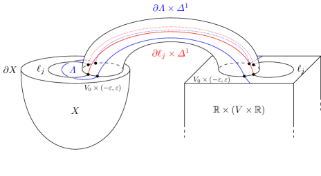
Figure 11. The definition of $CE^{\ast}(\varLambda,V;X)$ is given by the Chekanov–Eliashberg dg-algebra of the (non-compact) Legendrian submanifold $\varSigma_{\varLambda}$ which is shown in the figure.

Definition 2.26 ([AE22, Section 6.1]).

Let $(X,V)$ be a Weinstein pair, and let $\varLambda$ be a Legendrian submanifold relative to $V$. Let $\varSigma_{\varLambda}\mathrel{\mathop{\mathchar 58\relax}}=\varLambda\sqcup_{\partial\varLambda\times\left\{-1\right\}}(\partial\varLambda\times\varDelta^{1})\sqcup_{\partial\varLambda\times\left\{1\right\}}(\left\{0\right\}\times\partial\varLambda\times{\mathbb{R}})\subset\partial X_{V_{0}}$ denote the union of top attaching spheres of $X_{V}$, and define

$$CE^{\ast}(\varLambda,V;X)\mathrel{\mathop{\mathchar 58\relax}}=CE^{\ast}(\varSigma_{\varLambda};X_{V_{0}}).$$

Lemma 2.27 ([AE22, Lemma 6.1]).

There is a dg-subalgebra of $CE^{\ast}(\varLambda,V;X)$ which is canonically quasi-isomorphic to $CE^{\ast}(\partial\varLambda;V_{0})$.

Definition 2.28 ([Asp23, Definition 4.1]).

A Legendrian submanifold relative to a simplicial decomposition is a collection $\boldsymbol{\varLambda}$ consisting of one embedded Legendrian $(n-k-1)$-submanifold-with-boundary-and-corners $\varLambda_{\sigma_{k}}\subset\partial V^{(k)}_{\sigma_{k}}$ for each $\sigma_{k}\in C$, such that

$$\partial\varLambda_{\sigma_{k}}=\#\boldsymbol{\varLambda}_{\supsetneq\sigma_{k}}\subset\partial\#\boldsymbol{V}_{\supsetneq\sigma_{k}}\,,$$

where $\boldsymbol{\varLambda}_{\supsetneq\sigma_{k}}\mathrel{\mathop{\mathchar 58\relax}}=\left\{\varLambda_{\sigma_{i}}\right\}_{\sigma_{i}\supsetneq\sigma_{k}}$, and $\#\boldsymbol{\varLambda}_{\supsetneq\sigma_{k}}$ is defined recursively in analogy to the Weinstein manifold $\#\boldsymbol{V}_{\supsetneq\sigma_{k}}$, see [Asp23, Section 2.2].

We now extend these definitions to simplicial decompositions of Weinstein pairs.

Definition 2.29.

A Legendrian submanifold relative to a simplicial decomposition of a Weinstein pair $(X,P)$ consists of a Legendrian submanifold $\boldsymbol{\varLambda}^{\prime}$ relative to the given simplicial decomposition of $P$ and a collection $\boldsymbol{\varLambda}$ consisting of one embedded Legendrian $(n-k-1)$-submanifold-with-boundary-and-corners $\varLambda_{\sigma_{k}}\subset\partial V_{\sigma_{k}}^{(k)}$ for each $\sigma_{k}^{\prime}\in C^{\prime}$ such that

$$\partial\varLambda_{\sigma_{k}}=\#(\boldsymbol{\varLambda}^{\prime}_{\supset\sigma_{k}^{\prime}}\sqcup_{i}\boldsymbol{\varLambda}_{\supsetneq\sigma_{k}})\supset\partial\#(\boldsymbol{V}^{\prime}_{\supset\sigma_{k}^{\prime}}\sqcup_{i}\boldsymbol{V}_{\supsetneq\sigma_{k}})\,,$$

where $\boldsymbol{\varLambda}^{\prime}_{\supset\sigma_{k}^{\prime}}\sqcup_{i}\boldsymbol{\varLambda}_{\supsetneq\sigma_{k}}\mathrel{\mathop{\mathchar 58\relax}}=\boldsymbol{\varLambda}^{\prime}_{\supset\sigma_{k}^{\prime}}\cup\boldsymbol{\varLambda}_{\supsetneq\sigma_{k}}$.

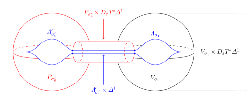
Figure 12. An example of a Legendrian submanifold relative to a simplicial decomposition with $C^{\prime}=\varDelta^{1}$. The ambient manifold in view is $V_{\sigma_{0}}$ and the Legendrian submanifold $\partial\varLambda_{\sigma_{0}}=\varLambda^{\prime}_{\sigma_{0}^{\prime}}\#_{\varLambda^{\prime}_{\sigma_{1}^{\prime}}}\varLambda_{\sigma_{1}}$ which is shown in the figure.

Remark 2.30.

We point out that Legendrian submanifolds-with-boundary was also studied from the point of view of sutured contact manifolds by Dattin [Dat22], which is expected to generalize the results in this paper. From the point of view of sutured contact manifolds, Weinstein pairs $(X,V)$ give rise to a balanced sutured contact manifold, and in that special case, we expect that our definition of $CE^{\ast}(\varLambda,V;X)$ coincides with the definition in [Dat22].

Definition 2.31.

Extend the various Legendrian submanifolds-with-boundary-and-corners in $\boldsymbol{\varLambda}$ over the simplicial handles used to construct $X$ (cf. [Asp23, Definition 4.2]). This yields a Legendrian submanifold $\overline{\varLambda}\subset\partial X$ relative to $P$. We call $\overline{\varLambda}$ the $\boldsymbol{V}$-completion of $\boldsymbol{\varLambda}$.

Definition 2.32.

Let $((C,C^{\prime}),(\boldsymbol{V},\boldsymbol{V}^{\prime}))$ be a simplicial decomposition of the Weinstein pair $(X,P)$ and let $\boldsymbol{\varLambda}$ be a Legendrian submanifold relative to $((C,C^{\prime}),(\boldsymbol{V},\boldsymbol{V}^{\prime}))$. Define

$$CE^{\ast}(\boldsymbol{\varLambda};(X,P))\mathrel{\mathop{\mathchar 58\relax}}=CE^{\ast}(\overline{\varLambda},P;X),$$

where $\overline{\varLambda}$ is the $\boldsymbol{V}$-completion of $\boldsymbol{\varLambda}$.

We now turn to the analogous results for Legendrian submanifolds relative to simplicial decompositions of Weinstein pairs. Let $\varSigma(\boldsymbol{h})$ denote the union of top attaching spheres of the simplicial handle $P\times D_{\varepsilon}T^{\ast}\varDelta^{1}$ used to construct $X_{P}$.

We use the notation $X\to Y\to Z$ to mean a word of Reeb chords $vw$ where $w$ is a Reeb chord from $X$ to $Y$, and $w$ is a Reeb chord from $Y$ to $Z$. With the same notation as in [Asp23, Section 4.1] we have the following.

Lemma 2.33.

Assume $((C,C^{\prime}),(\boldsymbol{V},\boldsymbol{V}^{\prime}))$ is a simplicial decomposition of $(X,P)$. For all $\mathfrak{a}>0$ there exists some $\delta>0$ and an arbitrarily small perturbation of $P$ such that for all $0<\boldsymbol{\varepsilon}<\delta$, the generators of $CE^{\ast}(\boldsymbol{\varLambda};(X,P))$ are in one-to-one correspondence with composable words of Reeb chords of action $<\mathfrak{a}$ which are of the form $\boldsymbol{\varLambda}\to\boldsymbol{\varLambda}$ or

$$\boldsymbol{\varLambda}\to\varSigma(\boldsymbol{h})\to\cdots\to\varSigma(\boldsymbol{h})\to\boldsymbol{\varLambda}.$$

The differential on $CE^{\ast}(\boldsymbol{\varLambda};(X,P))$ is induced by the differential in the Chekanov–Eliashberg dg-algebra of $\varSigma_{\varLambda}\cup\varSigma(\boldsymbol{h})\subset\partial(X_{P})_{0}$.

Proof.

The proof follows by the surgery description comparing generators before and after attachment of critical handles, see [Asp23, Lemma 4.5] and [BEE12, Theorem 5.10]. ∎

Theorem 2.34.

Suppose $\boldsymbol{\varLambda}$ is a Legendrian submanifold relative to the simplicial decomposition $((C,C^{\prime}),(\boldsymbol{V},\boldsymbol{V}^{\prime}))$ of the Weinstein pair $(X,P)$. Suppose that there are no Reeb chords from $\overline{\varLambda}$ to $\varSigma(\boldsymbol{h})$ or that there are no Reeb chords from $\varSigma(\boldsymbol{h})$ to $\overline{\varLambda}$. Then there is a quasi-isomorphism of dg-algebras

$$CE^{\ast}(\boldsymbol{\varLambda};(X,P))\cong\operatorname*{colim}_{\sigma_{k}^{\prime}\in C^{\prime}}CE^{\ast}(\boldsymbol{\varLambda};(X(\sigma_{k}),P(\sigma_{k}^{\prime}))).$$

Proof.

By the surgery description of the generators in 2.33, the only Reeb chords of $\boldsymbol{\varLambda}$ of action $<\mathfrak{a}$ are $\boldsymbol{\varLambda}\to\boldsymbol{\varLambda}$ in $\partial X_{P_{0}}$. The proof now follows by repeating the idea of [Asp23, Theorem 2.33]. ∎

Now we restrict attention to $C=C^{\prime}=\varDelta^{1}$. Consider the case when $\varLambda$ is a Legendrian in $(X,P)\mathrel{\mathop{\mathchar 58\relax}}=(X_{1},P_{1})\#_{V}(X_{2},P_{2})$ where $P_{i}=W_{i}\#_{Q_{i}}V$ for $i\in\left\{1,2\right\}$, where we assume that $W_{i}$ and $R_{i}$ are subcritical. Consider the Legendrian submanifold $\varLambda=\varLambda_{1}\#_{\partial\varLambda_{V}}\varLambda_{2}$ in $\partial X$ relative to $P$, where $\partial\varLambda_{V}$ is the common boundary of $\partial\varLambda_{1}$ and $\partial\varLambda_{2}$ along $V$ in $P_{1}$ and $P_{2}$, respectively. Here $\varLambda_{i}$ is a Legendrian submanifold in $\partial X_{i}$ relative to $P_{i}$. Let $\varSigma(h)=\ell_{V}\sqcup(\partial\ell_{V}\times\varDelta^{1})\sqcup\ell_{V}$ be the top attaching sphere of the basic building block $V\times T^{\ast}\varDelta^{1}$ used to construct $X$, where $\ell_{V}$ is the union of top core disks of a handle decomposition of $V$ (and hence of each $P_{i}$ by the subcriticality assumption on $W_{i}$ and $Q_{i}$).

Let $\mathbb{F}$ be a field and let $\boldsymbol{k}\mathrel{\mathop{\mathchar 58\relax}}=\bigoplus_{i\in\pi_{0}(\varLambda)}\mathbb{F}e_{i}$ where $\left\{e_{i}\right\}_{i\in\pi_{0}(\varLambda)}$ is a set of mutually orthogonal idempotents. We give an alternative description of the dg-algebra described in 2.33 as a $\boldsymbol{k}$-module. Let $\mathcal{A}_{i\to V}$ ($\mathcal{A}_{V\to i}$) denote the right (left) $CE^{\ast}((V,h);X_{i})$-module freely generated by the Reeb chords from $\varLambda_{i}$ to $\ell_{V}$ and $\partial\varLambda_{V}$ to $\partial\ell_{V}$ ($\ell_{V}$ to $\varLambda_{i}$ and $\partial\ell_{V}$ to $\partial\varLambda_{V}$) in $\partial X_{i}$. Similarly we let $\mathcal{A}_{i\to i}$ denote the algebra generated by Reeb chords from $\varLambda_{i}$ to $\varLambda_{i}$ in $\partial X_{i}$ and $\partial\varLambda_{i}$ to $\partial\varLambda_{i}$ in $\partial P_{i}$. Define the following modules over $\boldsymbol{k}$. Let $\mathcal{A}_{V}$ denote the set of Reeb chords of $\ell_{V}$ in $\partial X_{i}$ for $i\in\left\{1,2\right\}$. Let $\overline{\mathcal{A}}_{i\to V}$ ($\overline{\mathcal{A}}_{V\to j}$) be the right (left) module over the free algebra on $\mathcal{A}_{V}$ generated by the Reeb chords from $\varLambda_{i}$ to $\ell_{V}$ ($\ell_{V}$ to $\varLambda_{j}$).

$$\mathcal{A}_{i\to V\to i} \mathrel{\mathop{\mathchar 58\relax}}=\mathcal{A}_{i\to V}\otimes_{CE^{\ast}((V,h);X_{i})}\mathcal{A}_{V\to i},\quad i\in\left\{1,2\right\}$$

$$\mathcal{A}_{i\to V\to j} \mathrel{\mathop{\mathchar 58\relax}}=\overline{\mathcal{A}}_{i\to V}\otimes_{\mathcal{A}_{V}}\overline{\mathcal{A}}_{V\to j},\quad i\neq j\in\left\{1,2\right\}.$$

Lemma 2.35.

1. The dg-algebra $CE^{\ast}(\varLambda_{i},P_{i};X_{i})$ is quasi-isomorphic to the free dg-algebra generated by the set $\mathcal{A}_{i\to i}\cup\mathcal{A}_{i\to V\to i}$ and differential induced by the differential in the Chekanov–Eliashberg dg-algebra of $\varSigma_{V}(h)\cup\varLambda\subset\partial X_{V_{0}}$.

2. The dg-algebra $CE^{\ast}(\varLambda,P;X)$ is quasi-isomorphic to the free dg-algebra generated by the set

   $$\mathcal{A}_{1\to 1}\cup\mathcal{A}_{2\to 2}\cup\bigcup_{i,j\in\left\{1,2\right\}}\mathcal{A}_{i\to V\to j}$$

   and differential induced by the differential in the Chekanov–Eliashberg dg-algebra of $\varSigma_{V}(h)\cup\varLambda\subset\partial X_{V_{0}}$.

Proof.

Follows from the definition of $\mathcal{A}_{i\to i}$, $\mathcal{A}_{i\to V\to j}$ and 2.34. ∎

In the following, we let $A\ast B$ and $A\ast_{C}B$ denote the free product and amalgamated free product of two algebras $A$ and $B$ (over $C$), respectively. For $\mathcal{S}$ a set, we let $\left\langle\mathcal{S}\right\rangle$ denote the free associative non-commutative algebra generated by $\mathcal{S}$.

Corollary 2.36.

1. We have a quasi-isomorphism of dg-algebras

   $$CE^{\ast}(\varLambda_{i},P_{i};X_{i})\cong\left\langle\mathcal{A}_{i\to i}\right\rangle\ast\left\langle\mathcal{A}_{i\to V\to i}\right\rangle.$$

2. We have a quasi-isomorphism of dg-algebras

   $$CE^{\ast}(\varLambda,P;X)\cong CE^{\ast}(\varLambda_{1},P_{1};X_{1})\ast_{CE^{\ast}(\partial\varLambda_{V};V)}CE^{\ast}(\varLambda_{2},P_{2};X_{2})\ast\left\langle\mathcal{A}_{1\to V\to 2}\right\rangle\ast\left\langle\mathcal{A}_{2\to V\to 1}\right\rangle.$$

Proof.

This is simply a reformulation of 2.35, with the extra observation in item (2) that $CE^{\ast}(\partial\varLambda_{V};V)$ is quasi-isomorphic to dg-algebra generated by words of Reeb chords $\partial\varLambda_{V}\to\partial\ell_{V}\to\cdots\to\partial\ell_{V}\to\partial\varLambda_{V}$ (see [AE22, Proposition 6.3]). ∎

Remark 2.37.

1. Note that neither $\left\langle\mathcal{A}_{1\to V\to 2}\right\rangle$ nor $\left\langle\mathcal{A}_{2\to V\to 1}\right\rangle$ is a dg-algebra when equipped with the differential from $CE^{\ast}(\varLambda,P;X)$.

2. When $V$ is assumed to be subcritical we have $\mathcal{A}_{1\to V\to 2}=\mathcal{A}_{2\to V\to 1}=\varnothing$, and then 2.36 gives a special case of 2.34 when $C=C^{\prime}=\varDelta^{1}$.

3. Additionally, when $P=\varnothing$, and $V$ is assumed to be subcritical, then 2.36 recovers [AE22, Theorem 1.3] and a special case of [Asp23, Theorem 1.1].

Remark 2.38.

The free product and amalgamated free products used in 2.36 are both special cases of colimits in the category $\mathbf{a}$ which consists of associative, non-commutative, non-unital algebras over varying non-unital rings. Namely, there is a forgetful functor $\mathbf{dga}\to\mathbf{a}$ by forgetting the differential and grading, which means that all colimits are preserved because forgetful functors are left adjoints. The free product is the coproduct in $\mathbf{a}$ and the amalgamated free product is the pushout in $\mathbf{a}$. Colimits of free algebras in this category are again free algebras, generated by the union of the generators.

3. Tangle contact homology and gluing formulas

In this section we apply the results of Section 2 to define tangle contact homology and obtain gluing results for knot contact homology.

From now on and throughout the paper we let ${\mathbb{R}}^{3}_{x\geq 0}\mathrel{\mathop{\mathchar 58\relax}}=\left\{(x,y,z)\in{\mathbb{R}}^{3}\;|\;x\geq 0\right\}$, and we only consider metrics on ${\mathbb{R}}^{3}_{x\geq 0}$ such that $\partial{\mathbb{R}}^{3}_{x\geq 0}\subset{\mathbb{R}}^{3}_{x\geq 0}$ is not totally geodesic.

3.1. Unframed knot contact homology

In this section we first discuss the unframed knot contact homology and how the results of [AE22, Asp23] yields gluing formulas for the unframed version of knot contact homology.

Definition 3.1 (Tangle).

An $r$-component tangle in ${\mathbb{R}}^{3}_{x\geq 0}$ is a proper embedding

$$T\colon\left\{1,\ldots,r\right\}\times[-1,1]\longrightarrow{\mathbb{R}}^{3}_{x\geq 0}$$

such that $T(k,\pm 1)\subset\left\{y^{2}+z^{2}=1\right\}\subset\partial{\mathbb{R}}^{3}_{x\geq 0}$ for all $k\in\left\{1,\ldots,r\right\}$. We call $\bigcup_{k=1}^{r}\{T(k,1),T(k,-1)\}$ the boundary of $T$ and denote it by $\partial T$.

By abuse of notation we often also refer to the image of $T$ as an $r$-component tangle.

Remark 3.2.

In general we also allow components of a tangle to have empty boundary, but for notational simplicity we assume that each component of a tangle has boundary.

Definition 3.3 (Ambient isotopy).

We say that two tangles $T_{1}$ and $T_{2}$ are equivalent if they are ambient isotopic. That is, if there exists an isotopy $h_{t}\colon{\mathbb{R}}^{3}_{x\geq 0}\longrightarrow{\mathbb{R}}^{3}_{x\geq 0}$ such that

1. $h_{0}=\operatorname{id}$

2. $\mathinner{h_{1}\rvert}_{T_{1}}=T_{2}$

3. $\mathinner{h_{t}\rvert}_{\partial T_{1}}=\partial T_{2}$ such that $\mathinner{h_{t}\rvert}_{\partial T_{1}}\subset\left\{y^{2}+z^{2}=1\right\}\subset\partial{\mathbb{R}}^{3}_{x\geq 0}$ for all $t\in[0,1]$.

Definition 3.4 (Trivial tangle).

We say that an $r$-component tangle $T$ in ${\mathbb{R}}^{3}_{\geq 0}$ is trivial if it bounds $r$ disjoint embedded half-disks in ${\mathbb{R}}^{3}_{x\geq 0}$ whose $r$ boundary arcs are embedded and disjoint in $\left\{y^{2}+z^{2}=1\right\}\subset{\mathbb{R}}^{3}_{x=0}$.

Remark 3.5.

Be aware that our notion of a trivial tangle may not be standard terminology. It is equivalent to there existing a projection in which the tangle diagram does not have any crossings.

Assumption 3.6.

Tangles meet $\partial{\mathbb{R}}^{3}_{x\geq 0}$ orthogonally, and the geodesic binormal chords of a tangle are isolated.

Remark 3.7.

Note that 3.6 does not lose generality. It can always be achieved by small perturbations of the tangle and the given metric on ${\mathbb{R}}^{3}_{x\geq 0}$.

Definition 3.8 (Gluing of tangles).

Let $T_{1}$ and $T_{2}$ be two $r$-component tangles in ${\mathbb{R}}^{3}_{x\geq 0}$. The gluing of $T_{1}$ and $T_{2}$ is defined to be the link obtained by gluing the two copies of ${\mathbb{R}}^{3}_{x\geq 0}$ together along their common boundary by the identity map (possibly after an isotopy of $\partial{\mathbb{R}}^{3}_{x\geq 0}$ which matches up the boundaries of the two tangles).

Definition 3.9 (Knot contact homology following Ekholm–Etnyre–Ng–Sullivan).

In previous work of Ekholm–Etnyre–Ng–Sullivan [EENS13], knot contact homology of an $r$-component link was defined as

$$KCC^{\ast}_{\text{EENS}}(K)\mathrel{\mathop{\mathchar 58\relax}}=CE^{\ast}(\varLambda_{K},{\mathbb{Z}}[\lambda_{1}^{\pm 1},\mu_{1}^{\pm 1},\ldots,\lambda_{r}^{\pm 1},\mu_{r}^{\pm 1}];T^{\ast}{\mathbb{R}}^{3}),$$

where $\lambda_{1},\mu_{1},\ldots,\lambda_{r},\mu_{r}$ is a basis of $H_{1}(\varLambda_{K})$ consisting of longitude classes and meridian classes, respectively.

Remark 3.10.

We consider the fully non-commutative version of knot contact homology in which the generators $\lambda_{i}^{\pm 1}$ and $\mu_{i}^{\pm 1}$ for $i\in\left\{1,\ldots,r\right\}$ in 3.9 are declared to not commute with Reeb chord generators.

Definition 3.11 (Unframed knot contact homology of a link).

For a link $K\subset{\mathbb{R}}^{3}$ we define

$$KCC_{u}^{\ast}(K)\mathrel{\mathop{\mathchar 58\relax}}=CE^{\ast}(\varLambda_{K};T^{\ast}{\mathbb{R}}^{3})=\mathinner{KCC^{\ast}_{\text{EENS}}(K)\rvert}_{\lambda_{1}=\cdots\lambda_{r}=\mu_{1}=\cdots\mu_{r}=1}.$$

Let $T$ be a tangle in ${\mathbb{R}}^{3}_{x\geq 0}$ and let $H\mathrel{\mathop{\mathchar 58\relax}}=\partial{\mathbb{R}}^{3}_{x\geq 0}$. After convex completion of the (open) Weinstein sector $T^{\ast}{\mathbb{R}}^{3}_{x\geq 0}$ we obtain the Weinstein pair $(\widetilde{T^{\ast}{\mathbb{R}}^{3}_{x\geq 0}},T^{\ast}H)$ [GPS20, Section 2.7]. Note that in our notation $\widetilde{T^{\ast}{\mathbb{R}}^{3}_{x\geq 0}}$ is still an open Weinstein sector. We convex complete along the horizontal boundary $\partial T^{\ast}{\mathbb{R}}^{3}_{x\geq 0}=T^{\ast}\mathinner{{\mathbb{R}}^{3}\rvert}_{x=0}$ only.

The unit conormal bundle of $T$ is a Legendrian submanifold $\varLambda_{T}\subset\partial_{\infty}\widetilde{T^{\ast}{\mathbb{R}}^{3}_{x\geq 0}}$ relative to $T^{\ast}H$ in the sense of 2.25.

Definition 3.12 (Unframed tangle contact homology algebra).

Let $T$ be a tangle in ${\mathbb{R}}^{3}_{x\geq 0}$. We define the unframed tangle contact homology algebra of $T$ as

$$KCC_{u}^{\ast}(T)\mathrel{\mathop{\mathchar 58\relax}}=CE^{\ast}(\varLambda_{T},T^{\ast}H;\widetilde{T^{\ast}{\mathbb{R}}^{3}_{x\geq 0}}).$$

The homology of the dg-algebra $KCC^{\ast}_{u}(T)$ is called unframed tangle contact homology.

Lemma 3.13.

There is a dg-subalgebra of $KCC_{u}^{\ast}(T)$ which is canonically quasi-isomorphic to $KCC_{u}^{\ast}(\partial T)$.

Proof.

By definition $KCC_{u}^{\ast}(T)=CE^{\ast}(\varLambda_{T},T^{\ast}H;\widetilde{T^{\ast}{\mathbb{R}}^{3}_{x\geq 0}})$, and by 2.27 this dg-algebra contains a dg-subalgebra which is canonically quasi-isomorphic to $CE^{\ast}(\partial\varLambda_{T},T^{\ast}H)$, and since $\partial\varLambda_{T}=\varLambda_{\partial T}$ in $ST^{\ast}H$ the result follows. ∎

3.2. Knot contact homology for links

In this section we extend the definition of the fully non-commutative knot contact homology to a family of such homologies, depending on a choice of a handle decomposition $h$ of a small cotangent neighborhood of the unit conormal torus in $ST^{\ast}{\mathbb{R}}^{3}$. For certain choices of $h$ this definition recovers the Ekholm–Etnyre–Ng–Sullivan fully non-commutative knot contact homology defined in [EENS13, CELN17, ENS18].

Definition 3.14 (Knot contact homology for links).

Let $K\subset{\mathbb{R}}^{3}$ be a link. Define

$$KCC^{\ast}(K,h)\mathrel{\mathop{\mathchar 58\relax}}=CE^{\ast}((N(\varLambda_{K}),h);T^{\ast}{\mathbb{R}}^{3}),$$

where $N(\varLambda_{K})\cong D_{\varepsilon}T^{\ast}\varLambda_{K}$ is a small cotangent neighborhood of the unit conormal bundle of $K$, together with a chosen handle decomposition $h$.

In general we have that the quasi-isomorphism class of $KCC^{\ast}(K,h)$ depends on the handle decomposition $h$ as can be observed by [AE22, Example 7.4 and Example 7.5].

Lemma 3.15.

Let $h_{1}$ and $h_{2}$ be two handle decompositions of $N(\varLambda_{K})$.

1. $KCC^{\ast}(K,h_{1})$ and $KCC^{\ast}(K,h_{2})$ are derived Morita equivalent.

2. There is an isomorphism of algebras $HH_{\ast}(KCC^{\ast}(K,h_{1}))\cong HH_{\ast}(KCC^{\ast}(K,h_{2}))$, where $HH_{\ast}$ denotes Hochschild homology.

3. Denote the subcollection of top handles of $h_{1}$ and $h_{2}$ by $h^{\mathrm{top}}_{1}$ and $h^{\mathrm{top}}_{2}$ respectively. If the core disks in $h^{\mathrm{top}}_{1}$ and $h^{\mathrm{top}}_{2}$ are related by a Legendrian isotopy $h^{\mathrm{top}}_{t}$ in $T^{\ast}{\mathbb{R}}^{3}$ with the property that $\partial h^{\mathrm{top}}_{t}$ is a Legendrian isotopy of $\partial h^{\mathrm{top}}_{1}$ and $\partial h^{\mathrm{top}}_{2}$ in $\partial N(\varLambda_{K})_{0}$ then we have that $KCC^{\ast}(K,h_{1})$ and $KCC^{\ast}(K,h_{2})$ are dg-homotopy equivalent.

Proof.

The proof of (1) and (2) were sketched in [AE22, Remark 1.5]. For the sake of completeness we summarize the proofs below.

1. By the surgery formula [AE22, Theorem 1.1] we have a quasi-isomorphism

   $$CE^{\ast}((N(\varLambda_{K}),h);T^{\ast}{\mathbb{R}}^{3})\cong CW^{\ast}(C(h);(T^{\ast}{\mathbb{R}}^{3})_{\varLambda_{K}}),$$

   where $(T^{\ast}{\mathbb{R}}^{3})_{\varLambda_{K}}$ is $T^{\ast}{\mathbb{R}}^{3}$ stopped at $\varLambda_{K}$ and where $C(h)$ is the union of cocore disks of the top handle of $(T^{\ast}{\mathbb{R}}^{3})_{\varLambda_{K}}$ depending on the handle decomposition $h$ of $N(\varLambda_{K})$. The wrapped Fukaya category $\mathcal{W}((T^{\ast}{\mathbb{R}}^{3})_{\varLambda_{K}})$ is generated by the summands of $C(h)$ by [CDRGG17, Theorem 1.1] and [GPS22, Theorem 1.13]. As the derived module category is independent of choice of a generating set, the result follows.

2. Attachment of the $1$-simplex handle $N(\varLambda_{K})_{0}\times D_{\varepsilon}T^{\ast}\varDelta^{1}$ gives rise to a natural geometric Weinstein cobordism with positive contact boundary $\partial(T^{\ast}{\mathbb{R}}^{3})_{\varLambda_{K}}$ and negative contact boundary $\partial T^{\ast}{\mathbb{R}}^{3}$. By [BEE12, Theorem 5.6] we have a quasi-isomorphism

   $$SH^{\ast}((T^{\ast}{\mathbb{R}}^{3})_{\varLambda_{K}})\cong HH_{\ast}(CE^{\ast}((N(\varLambda_{K}),h);T^{\ast}{\mathbb{R}}^{3}))\oplus SH^{\ast}(T^{\ast}{\mathbb{R}}^{3}).$$

   Since $SH^{\ast}((T^{\ast}{\mathbb{R}}^{3})_{\varLambda_{K}})$ and $SH^{\ast}(T^{\ast}{\mathbb{R}}^{3})$ does not depend on the handle decomposition $h$, it follows that the Hochschild homology of the Chekanov–Eliashberg dg-algebra also does not.

3. Such Legendrian isotopies of $h^{\text{top}}_{1}$ and $h^{\text{top}}_{2}$ induces a Legendrian isotopy $\varSigma(h_{1})\simeq\varSigma(h_{2})$ and the result follows from the invariance of the Chekanov–Eliashberg dg-algebra up to dg-homotopy equivalent under Legendrian isotopy, see [EN15, Appendix A] and [EO17, Corollary 5.17].

∎

Lemma 3.16.

The dg-homotopy equivalence class of the dg-algebra $KCC^{\ast}(K,h)$ is an ambient isotopy invariant of $K\subset{\mathbb{R}}^{3}$

Proof.

Ambient isotopies of $K$ induces Legendrian isotopies of $\varLambda_{K}$ which induces isotopies of Weinstein hypersurfaces $N(\varLambda_{K})\hookrightarrow\partial T^{\ast}{\mathbb{R}}^{3}$. Such isotopies gives Legendrian isotopies as in item (3) of 3.15. ∎

Theorem 3.17.

Let $K\subset{\mathbb{R}}^{3}$ be a link. If $h$ is a handle decomposition of $N(\varLambda_{K})$ such that each component of $N(\varLambda_{K})$ has a single top handle, then there is a quasi-isomorphism

$$KCC^{\ast}(K,h)\cong KCC_{\mathrm{EENS}}^{\ast}(K).$$

Proof.

By 2.16 it follows that $KCC^{\ast}(K,h)\cong CE^{\ast}\left(\varLambda_{K},\bigoplus_{i}C_{-\ast}(\varOmega\varLambda_{K_{i}});T^{\ast}{\mathbb{R}}^{3}\right)$. Since $\varLambda_{K_{i}}\cong T^{2}$ for each component $K_{i}$ of $K$ it follows that we have a quasi-isomorphism $C_{-\ast}(\varOmega\varLambda_{K_{i}})\cong{\mathbb{Z}}[H_{1}(\varLambda_{K_{i}})]$ for each $i$. We obtain the fully non-commutative knot contact homology by definition of the Chekanov–Eliashberg dg-algebra with loop space coefficients as in [EL17] in which generators corresponding to chains of based loops do not commute with Reeb chord generators. The result follows. ∎

3.3. Tangle contact homology

Given a tangle $T$ in ${\mathbb{R}}^{3}_{x\geq 0}$, its unit conormal bundle $\varLambda_{T}$ is a Legendrian relative to the Weinstein hypersurface $T^{\ast}H\hookrightarrow\widetilde{T^{\ast}{\mathbb{R}}^{3}_{x\geq 0}}$ in the sense of 2.25 where $H\mathrel{\mathop{\mathchar 58\relax}}=\partial{\mathbb{R}}^{3}_{x\geq 0}$. We consider handle decompositions $h$ of $N(\varLambda_{T})$ as induced by a Morse function on $\varLambda_{T}$ treated as a compact manifold-with-boundary. That is, $h$ consists of both standard Weinstein handles, and Weinstein half-handles, see [CDRGG17, Section 2.3]. The standard model for Weinstein half-handles is revealed by studying Morse theory on manifolds with boundary, see [BNR16] and [KM07, Section 2.4]. Let $V_{T}$ denote the subcritical part of $N(\varLambda_{T})$ with respect to the handle decomposition $h$ of $N(\varLambda_{T})$, and let $\ell_{T}$ be the union of core disks of the top handles in $h$. We have that $V_{T}$ is a Weinstein subsector of ${\mathbb{R}}^{3}_{x\geq 0}$ which meets $T^{\ast}H$ along $Q_{T}\mathrel{\mathop{\mathchar 58\relax}}=V_{T}\cap ST^{\ast}H$ since we assume that $T$ intersect $H$ orthogonally, see 3.6. After convex completion we have that $\ell_{T}$ is a Legendrian submanifold relative to the Weinstein pair $(\widetilde{T^{\ast}{\mathbb{R}}^{3}_{x\geq 0}},P_{T})$ in the sense of Section 2.4, where $P_{T}$ is the Weinstein hypersurface $P_{T}\mathrel{\mathop{\mathchar 58\relax}}=\widetilde{V_{T}}\#_{Q_{T}}T^{\ast}H\hookrightarrow\partial_{\infty}\widetilde{T^{\ast}{\mathbb{R}}^{3}_{x\geq 0}}$.

Definition 3.18 (Tangle contact homology).

Let $T$ be a tangle in ${\mathbb{R}}^{3}_{x\geq 0}$ and let $h$ be a handle decomposition of $N(\varLambda_{T})$. We define the tangle contact homology algebra of $T$ as

$$KCC^{\ast}(T,h)\mathrel{\mathop{\mathchar 58\relax}}=CE^{\ast}(\ell_{T},P_{T};\widetilde{T^{\ast}{\mathbb{R}}^{3}_{x\geq 0}}).$$

Lemma 3.19.

Let $h$ be a handle decomposition of $N(\varLambda_{T})$. The quasi-isomorphism class of the dg-algebra $KCC^{\ast}(T,h)$ is an ambient isotopy invariant of $T\subset{\mathbb{R}}^{3}_{x\geq 0}$.

Proof.

Ambient isotopies of $T$ induces Legendrian isotopies of the relative Legendrian submanifold $\ell_{T}$ in the sense of item (3) of 3.15. The result follows. ∎

Lemma 3.20.

Let $T$ be a tangle in ${\mathbb{R}}^{3}_{x\geq 0}$ and let $h$ be a handle decomposition of $N(\varLambda_{T})$. There is a dg-subalgebra of $KCC^{\ast}(T,h)$ which is canonically quasi-isomorphic to $KCC^{\ast}(\partial T,h_{\partial})$.

Proof.

First we note that by definition of $KCC^{\ast}(T,h)$ and by 2.27 there is a dg-subalgebra of $KCC^{\ast}(T,h)$ canonically quasi-isomorphic to $CE^{\ast}(\partial\ell_{T};P_{T})$ where

$$\partial\ell_{T}\simeq\mathinner{\partial\ell_{T}\rvert}_{\partial\widetilde{V_{T}}}\sqcup\underbrace{(\partial\ell_{T}\cap\partial Q_{T}\times\varDelta^{1})}_{=\mathrel{\mathop{\mathchar 58\relax}}\ell_{\partial T}}\sqcup\mathinner{\partial\ell_{T}\rvert}_{ST^{\ast}H}.$$

By construction we have $\partial\ell_{T}\subset\partial(\widetilde{V_{T}}\#_{Q_{T}}T^{\ast}H)$. By construction $Q_{T}\hookrightarrow\partial V_{T},\partial T^{\ast}H$ is subcritical. Thus by the same proof as [Asp23, Theorem 4.6] $CE^{\ast}(\partial\ell_{T};P_{T})$ is quasi-isomorphic to the colimit of the following diagram

$$\leavevmode\hbox to210.63pt{\vbox to49.8pt{\text{[drawing]}}}. {CE^{\ast}(\ell_{\partial T},Q_{T})} {CE^{\ast}(\mathinner{\partial\ell_{T}\rvert}_{ST^{\ast}H},Q_{T};T^{\ast}H)} {CE^{\ast}(\mathinner{\partial\ell_{T}\rvert}_{\partial\widetilde{V_{T}}},Q_{T};\widetilde{V_{T}})} {CE^{\ast}(\ell_{\partial T},Q_{T})} {CE^{\ast}(\mathinner{\partial\ell_{T}\rvert}_{ST^{\ast}H},Q_{T};T^{\ast}H)} {CE^{\ast}(\mathinner{\partial\ell_{T}\rvert}_{\partial\widetilde{V_{T}}},Q_{T};\widetilde{V_{T}})}$$

In particular we note that by definition $CE^{\ast}(\mathinner{\partial\ell_{T}\rvert}_{ST^{\ast}H},Q_{T};T^{\ast}H)=KCC^{\ast}(\partial T,h_{\partial})$, and this is a dg-subalgebra of $CE^{\ast}(\partial\ell_{T};P_{T})$ and hence of $KCC^{\ast}(T,h)$. ∎

3.4. Gluing formula

Let $T_{1}$ and $T_{2}$ be two tangles in ${\mathbb{R}}^{3}_{x\geq 0}$. Let $h_{1}$ and $h_{2}$ be a handle decomposition of $N(\varLambda_{T_{1}})$ and $N(\varLambda_{T_{2}})$, respectively, such that the handle decompositions $(h_{1})_{\partial}$ and $(h_{2})_{\partial}$ of the boundary $N(\partial\varLambda_{T})$ agree. Suppose that the gluing of the two tangles $T_{1}$ and $T_{2}$ gives a link $K$. This induces a gluing of $N(\varLambda_{T_{1}})$ and $N(\varLambda_{T_{2}})$ such that it respects the handle decompositions $h_{1}$ and $h_{2}$ in the sense that the boundary critical points along $N(\partial\varLambda_{T})$ match up after the gluing. This gives an induced handle decomposition on $N(\varLambda_{K})$ which we denoted by $h_{1}\#h_{2}$, and we call such $h_{1}$ and $h_{2}$ gluing compatible.

Let $h_{H}$ be a handle decomposition with a single top handle of $T^{\ast}H\cong T^{\ast}{\mathbb{R}}^{2}$ viewed as $B^{4}$ stopped at the unknot. Let $\ell_{H}$ denote the $2$-dimensional core disk in $h_{H}$ and let $\varSigma_{H}(h_{H})$ denote the $2$-dimensional attaching sphere of the handle $T^{\ast}H\times T^{\ast}\varDelta^{1}$ in $\left(\widetilde{T^{\ast}{\mathbb{R}}^{3}_{x\geq 0}}\right)_{T^{\ast}H}$, used in the definition of $KCC^{\ast}(T_{i},h_{i})$. We use the notation $\partial\ell_{H}^{1}$ to denote the $1$-dimensional core disk of a handle decomposition of $T^{\ast}(\text{unknot})$ such that by attaching a stop on the unknot using this handle decomposition, the top attaching sphere of $T^{\ast}{\mathbb{R}}^{2}$ becomes exactly $\partial\ell$, see Figure 13.

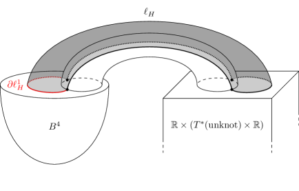
Figure 13. The $2$-dimensional core disk $\ell_{H}$ of the top handle of $T^{\ast}{\mathbb{R}}^{2}$ viewed as $B^{4}$ stopped at the unknot, with the $1$-dimensional core disk $\partial\ell_{H}^{1}$ in red.

Applying 2.33 we first describe the dg-algebras $KCC^{\ast}(T_{i},h_{i})\mathrel{\mathop{\mathchar 58\relax}}=CE^{\ast}(\ell_{T_{i}},P_{T_{i}};\widetilde{T^{\ast}{\mathbb{R}}^{3}_{x\geq 0}})$. Let $\varSigma_{T_{i}}(h_{i})=\ell_{T_{i}}\sqcup_{\partial\ell_{T_{i}}\times\left\{-1\right\}}(\partial\ell_{T_{i}}\times\varDelta^{1})\sqcup_{\partial\ell_{T_{i}}\times\left\{1\right\}}(\left\{0\right\}\times\partial\ell_{T_{i}}\times{\mathbb{R}})\subset\partial\left(\widetilde{T^{\ast}{\mathbb{R}}^{3}_{x\geq 0}}\right)_{P_{T_{i}}}$ be the non-compact Legendrian as in 2.26. Let $\partial\ell_{T_{i}}^{H}\mathrel{\mathop{\mathchar 58\relax}}=\partial\ell_{T_{i}}\cap B^{4}$, where $B^{4}$ is the subcritical part of $T^{\ast}H$, see Figure 14.

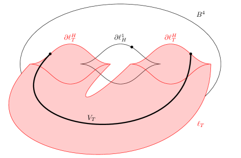
Figure 14. The figure shows the core disk $\ell_{T}$ of a handle decomposition $h$ of $N(\varLambda_{T})$ with subcritical part $V_{T}\cong D^{2}\times I$.

Lemma 3.21.

1. The dg-algebra $KCC^{\ast}(T,h)$ is quasi-isomorphic to the dg-algebra generated by composable words of Reeb chords of the form $\varSigma_{T}(h)\to\varSigma_{T}(h)$ and $\varSigma_{T}(h)\to\varSigma_{H}(h_{H})\to\cdots\to\varSigma_{H}(h_{H})\to\varSigma_{T}(h)$, and where the differential is the one induced from the differential of the Chekanov–Eliashberg dg-algebra of $\varSigma_{T}(h)\cup\varSigma_{H}(h_{H})\subset\partial\left(\widetilde{T^{\ast}{\mathbb{R}}^{3}_{x\geq 0}}\right)_{P_{T,0}}$.

2. The dg-subalgebra $KCC^{\ast}(\partial T,h_{\partial})\subset KCC^{\ast}(T_{i},h_{i})$ is quasi-isomorphic to the dg-algebra generated by composable words of Reeb chords of the form $\partial\ell_{T_{i}}^{H}\to\partial\ell_{T_{i}}^{H}$ and $\partial\ell_{T_{i}}^{H}\to\partial\ell_{H}^{1}\to\cdots\to\partial\ell_{H}^{1}\to\partial\ell_{T_{i}}^{H}$ and where the differential is the one induced from the differential of the Chekanov–Eliashberg dg-algebra of $\partial\ell_{T_{i}}^{H}\cup\partial\ell_{H}^{1}\subset\partial P_{T_{i}}$.

Proof.

This is a special case of 2.33 and [Asp23, Theorem 4.6]. ∎

After gluing two tangles $T_{1},T_{2}\subset{\mathbb{R}}^{3}_{x\geq 0}$ to a link $K\subset{\mathbb{R}}^{3}$ we obtain the following description of $KCC^{\ast}(K,h)$ in terms of $KCC^{\ast}(T_{i},h_{i})$ and $KCC^{\ast}(\partial T,h_{\partial})$. After gluing the two pairs $(\widetilde{T^{\ast}{\mathbb{R}}^{3}_{x\geq 0}},P_{T_{1}})$ and $(\widetilde{T^{\ast}{\mathbb{R}}^{3}_{x\geq 0}},P_{T_{2}})$ along their common Weinstein subhypersurface $T^{\ast}H$ we obtain the Weinstein pair $(T^{\ast}{\mathbb{R}}^{3},P)$ where $P\mathrel{\mathop{\mathchar 58\relax}}=\widetilde{V}_{T_{1}}\#_{Q_{T}}\widetilde{V}_{T_{2}}$ with notation as in Section 3.3. Let $\varSigma_{P}(h)$ denote the union of the top attaching spheres of the handle $T^{\ast}H\times T^{\ast}\varDelta^{1}$ used in the construction of the pair $(T^{\ast}{\mathbb{R}}^{3},P)$. Let $\ell_{K}$ denote the result of gluing $\ell_{T_{1}}$ and $\ell_{T_{2}}$ along their common boundary in $\partial B^{4}$ over the handle $B^{4}\times T^{\ast}\varDelta^{1}$. Furthermore let $\varSigma_{P}(h)$ and $\varSigma_{K}(h_{1}\#h_{2})$ denote the corresponding Legendrians after stopping $T^{\ast}{\mathbb{R}}^{3}$ at $P$.

Lemma 3.22.

The dg-algebra $KCC^{\ast}(K,h_{1}\#h_{2})$ is quasi-isomorphic to the dg-algebra generated by composable words of Reeb chords of the form $\varSigma_{K}(h_{1}\#h_{2})\to\varSigma_{K}(h_{1}\#h_{2})$ and $\varSigma_{K}(h_{1}\#h_{2})\to\varSigma_{P}(h)\to\cdots\to\varSigma_{P}(h)\to\varSigma_{K}(h_{1}\#h_{2})$, and where the differential is the one induced from the differential of the Chekanov–Eliashberg dg-algebra of $\varSigma_{K}(h_{1}\#h_{2})\cup\varSigma_{P}(h)\subset\partial(T^{\ast}{\mathbb{R}}^{3})_{P_{0}}$.

Proof.

Follows immediately by the construction and from 2.33. ∎

We proceed to give a topological description of some of the generators appearing in 3.21.

Lemma 3.23.

Let $T\subset{\mathbb{R}}^{3}_{x\geq 0}$ be a tangle and let $h$ be a handle decomposition of $N(\varLambda_{T})$.

1. Reeb chords of the form $\ell_{T}\to\ell_{T}$ are in one-to-one correspondence with oriented binormal geodesic chords of $T\subset{\mathbb{R}}^{3}_{x\geq 0}$,

2. Composable words of Reeb chords of the form $\partial\ell_{T}^{H}\to\partial\ell_{T}^{H}$ or $\partial\ell_{T}^{H}\to\partial\ell_{H}^{1}\to\cdots\to\partial\ell_{H}^{1}\to\partial\ell_{T}^{H}$ are in one-to-one correspondence with oriented binormal geodesic chords of $\partial T\subset H$,

3. Reeb chords of the form $\ell_{H}\to\ell_{T}$ or $\ell_{T}\to\ell_{H}$ are in one-to-one correspondence with oriented binormal geodesic chords from $H$ to $T$ and $T$ to $H$ in ${\mathbb{R}}^{3}_{x\geq 0}$, respectively.

4. Reeb chords of the form $\ell_{H}\to\ell_{H}$ are in one-to-one correspondence with oriented binormal geodesic $H$ in ${\mathbb{R}}^{3}_{\geq 0}$.

Proof.

1. This follows from the fact that the Reeb flow in $ST^{\ast}{\mathbb{R}}^{3}_{x\geq 0}$ away from $x=0$ corresponds to geodesic flow in ${\mathbb{R}}^{3}_{x\geq 0}$.

2. This follows from 2.33, and in particular [AE22, Proposition 6.2].

3. This follows from the fact that the Reeb flow in $ST^{\ast}{\mathbb{R}}^{3}_{x\geq 0}$ away from $x=0$ corresponds to geodesic flow in ${\mathbb{R}}^{3}_{x\geq 0}$. By construction we have that the top attaching sphere $\ell_{H}$ of $T^{\ast}H$ in $\widetilde{T^{\ast}{\mathbb{R}}^{3}_{x\geq 0}}$ is the Legendrian lift of $H\subset{\mathbb{R}}^{3}_{x\geq 0}$ after convex completion. From this point of view, $H\subset T^{\ast}{\mathbb{R}}^{3}_{x\geq 0}$ behaves serves as the front projection of $\ell_{H}$, from which the correspondence follows.

4. This is the same proof as item (3).

∎

Let $\mathcal{G}_{\partial H}=CE^{\ast}(\partial\ell_{H},(B^{4})_{D^{2}})$, see Figure 13. We define $\mathcal{G}_{T\to H}$ ($\mathcal{G}_{H\to T}$) denote the right (left) module over the algebra $\mathcal{G}_{\partial H}$ generated by Reeb chords from $\ell_{T}$ to $\ell_{H}$ and $\partial\ell_{T}^{H}$ to $\partial\ell_{H}^{1}$ ($\ell_{H}$ to $\ell_{T}$ and $\partial\ell_{H}^{1}$ to $\partial\ell_{T}^{H}$). Similarly, let $\mathcal{G}_{T\to T}$ denote the set of Reeb chords of $\ell_{T}\subset\partial\widetilde{T}^{\ast}{\mathbb{R}}^{3}_{x\geq 0}$. We define

(3.1) $$\mathcal{G}_{T\to H\to T}\mathrel{\mathop{\mathchar 58\relax}}=\mathcal{G}_{T\to H}\otimes_{\mathcal{G}_{\partial H}}\mathcal{G}_{H\to T},$$

as modules. In the following we will only consider the underlying sets of $\mathcal{G}_{T\to T}$, $\mathcal{G}_{T\to H}$, $\mathcal{G}_{H\to T}$ and $\mathcal{G}_{T\to H\to T}$.

Corollary 3.24.

Let $T\subset{\mathbb{R}}^{3}_{x\geq 0}$ be a tangle and let $h$ be a handle decomposition of $N(\varLambda_{T})$.

1. Elements of $\mathcal{G}_{T\to T}$ are in one-to-one correspondence with oriented binormal geodesic chords of $T\subset{\mathbb{R}}^{3}_{x\geq 0}$.

2. Elements of $\mathcal{G}_{T\to H\to T}$ are in one-to-one correspondence with oriented binormal geodesic chords of $\partial T\subset H$ and words of oriented binormal geodesic chords in ${\mathbb{R}}^{3}_{x\geq 0}$ of the form $T\to H\to\cdots\to H\to T$.

Proof.

1. This is a reformulation of item (1) of 3.23.

2. By construction we have that elements of $\mathcal{G}_{T\to H\to T}$ consists of words of Reeb chords of the form

   1. $\partial\ell_{T}^{H}\to\partial\ell_{H}^{1}\to\cdots\to\partial\ell_{H}^{1}\to\partial\ell_{T}^{H}$, and

   2. $\ell_{T}\to\ell_{H}\to\cdots\to\ell_{H}\to\ell_{T}$.

   Note that there are no other words, because there are no Reeb chords of the form $\partial\ell_{H}^{1}\to\ell_{H}$ by construction, see [AE22, Section 2.2] and [Asp23, Section 2.1] for a discussion of Reeb flows in the standard building blocks that we are using.

   Words of the form (a) corresponds to oriented binormal geodesic chords of $T\subset{\mathbb{R}}^{3}_{x\geq 0}$ by item (2) of 3.23. Words of the form (b) corresponds to words of oriented binormal geodesic chords in ${\mathbb{R}}^{3}_{x\geq 0}$ of the form $T\to H\to\cdots\to H\to T$ by items (3) and (4) of 3.23.

∎

Theorem 3.25.

Let $T\subset{\mathbb{R}}^{3}_{x\geq 0}$ be a tangle. Let $h$ be a choice of handle decomposition of $N(\varLambda_{T})$. Then we have a quasi-isomorphism of dg-algebras

$$KCC^{\ast}(T,h)\cong\left\langle\mathcal{G}_{T\to T}\right\rangle\ast\left\langle\mathcal{G}_{T\to H\to T}\right\rangle.$$

Proof.

This follows from 2.36. Let us spell out the details. By item (1) of 3.21 we have that $KCC^{\ast}(T,h)$ is quasi-isomorphic to the dg-algebra generated by words of Reeb chords of the form $\varSigma_{T}(h)\to\varSigma_{T}(h)$ and $\varSigma_{T}(h)\to\varSigma_{H}(h_{H})\to\cdots\to\varSigma_{H}(h_{H})\to\varSigma_{T}(h)$. We need to show that such Reeb chords correspond to elements in the set $\mathcal{G}_{T\to T}\cup\mathcal{G}_{T\to H\to T}$.

It follows from studying the Reeb dynamics in the standard building block $V\times T^{\ast}\varDelta^{1}$ as defined in [AE22, Section 2.2] and [Asp23, Section 2.1]. Namely, there are no Reeb chords from $\partial\ell_{T}\times\varDelta^{1}\subset\partial_{\infty}(P_{T}\times T^{\ast}\varDelta^{1})$ to $\ell_{T}\subset\partial\widetilde{T^{\ast}{\mathbb{R}}^{3}_{x\geq 0}}$. Hence, after removing the top handles of $P_{T}$, the available words are of the form $\partial\ell_{T}^{H}\to\partial\ell_{H}^{1}\to\cdots\to\partial\ell_{H}^{1}\to\partial\ell_{T}^{H}$ or $\ell_{T}\to\ell_{H}\to\cdots\to\ell_{H}\to\ell_{T}$. ∎

Remark 3.26.

Neither $\mathcal{G}_{T\to T}$ nor $\mathcal{G}_{T\to T}$ become dg-algebras when equipped with the differential used in $KCC^{\ast}(T,h)$, however the free algebra becomes a dg-algebra when equipped with the differential used in $KCC^{\ast}(T,h)$.

Now let $T_{1}$ and $T_{2}$ be two tangles in ${\mathbb{R}}^{3}_{x\geq 0}$. As the discussion surrounding (3.1) we define $\mathcal{G}_{T_{i}\to T_{i}}$, $\mathcal{G}_{T_{i}\to H\to T_{i}}$ in the same way for $i\in\left\{1,2\right\}$. Additionally we define $\mathcal{G}_{H}$ to denote the set of Reeb chords of $\ell_{H}$ in either one of the two copies of $\widetilde{T^{\ast}{\mathbb{R}}^{3}_{x\geq 0}}$. Let $\overline{\mathcal{G}}_{T_{i}\to H}$ (and $\overline{\mathcal{G}}_{H\to T_{j}}$) be the right (left) module over the free algebra on $\mathcal{G}_{H}$ generated by Reeb chords from $\ell_{T_{i}}$ to $\ell_{H}$ ($\ell_{H}$ to $\ell_{T_{j}}$). Then define

(3.2) $$\mathcal{G}_{T_{i}\to H\to T_{j}}\mathrel{\mathop{\mathchar 58\relax}}=\overline{\mathcal{G}}_{T_{i}\to H}\otimes_{\mathcal{G}_{H}}\overline{\mathcal{G}}_{H\to T_{j}},$$

for $i\neq j\in\left\{1,2\right\}$.

Lemma 3.27.

Let $T_{1}\subset({\mathbb{R}}^{3}_{x\geq 0})_{1}$ and $T_{2}\subset({\mathbb{R}}^{3}_{x\geq 0})_{2}$ be two tangles. Elements of $\mathcal{G}_{T_{i}\to H\to T_{j}}$ for $i\neq j\in\left\{1,2\right\}$ are in one-to-one correspondence with words of oriented binormal geodesic chords in of the form $T_{i}\to H\to\cdots\to H\to T_{j}$, where “$H\to H$” is taken to mean an oriented binormal geodesic chord of $H$ in either of the two copies of ${\mathbb{R}}^{3}_{x\geq 0}$.

Proof.

This follows from 3.22 in combination with item (3) of 3.23. ∎

Theorem 3.28 (1.1).

Let $T_{1}$ and $T_{2}$ be two tangles in ${\mathbb{R}}^{3}_{x\geq 0}$ whose gluing is the link $K\subset{\mathbb{R}}^{3}$, where $H\mathrel{\mathop{\mathchar 58\relax}}=\partial{\mathbb{R}}^{3}_{x\geq 0}$. Let $h_{1}$ and $h_{2}$ be choices of handle decomposition of $N(\varLambda_{T_{1}})$ and $N(\varLambda_{T_{2}})$, respectively. Then we have a quasi-isomorphism of dg-algebras

$$KCC^{\ast}(K,h_{1}\#h_{2})\cong KCC^{\ast}(T_{1},h_{1})\ast_{KCC^{\ast}(\partial T,h_{\partial})}KCC^{\ast}(T_{2},h_{2})\ast\left\langle\mathcal{G}_{T_{1}\to H\to T_{2}}\right\rangle\ast\left\langle\mathcal{G}_{T_{2}\to H\to T_{1}}\right\rangle,$$

where the right hand side is equipped with the same differential as in $KCC^{\ast}(K,h_{1}\#h_{2})$.

Proof.

This follows from 2.36. Let us spell out the details. By 3.22 and the same discussion regarding Reeb dynamics as in the proof of 3.25 we see that

$$KCC^{\ast}(K,h_{1}\#h_{2}) \cong\left\langle\mathcal{G}_{T_{1}\to T_{1}}\cup\mathcal{G}_{T_{2}\to T_{2}}\cup\mathcal{G}_{T_{1}\to H\to T_{1}}\cup\mathcal{G}_{T_{1}\to H\to T_{2}}\cup\mathcal{G}_{T_{2}\to H\to T_{1}}\cup\mathcal{G}_{T_{2}\to H\to T_{2}}\right\rangle$$

$$=\left\langle\mathcal{G}_{T_{1}\to T_{1}}\cup\mathcal{G}_{T_{1}\to H\to T_{1}}\cup\mathcal{G}_{T_{2}\to T_{2}}\cup\mathcal{G}_{T_{2}\to H\to T_{2}}\right\rangle\ast\left\langle\mathcal{G}_{T_{1}\to H\to T_{2}}\right\rangle\ast\left\langle\mathcal{G}_{T_{2}\to H\to T_{1}}\right\rangle.$$

Now $\mathcal{G}_{T_{1}\to H\to T_{1}}$ and $\mathcal{G}_{T_{1}\to H\to T_{1}}$ has a common subset consisting of words of oriented binormal geodesic chords of $\partial T\subset H$. The dg-algebra generated by such is quasi-isomorphic with $KCC^{\ast}(\partial T,h_{\partial})$ when equipped with the differential of $KCC^{\ast}(K,h_{1}\#h_{2})$ by 3.21. Hence

$$\left\langle\mathcal{G}_{T_{1}\to T_{1}}\cup\mathcal{G}_{T_{1}\to H\to T_{1}}\cup\mathcal{G}_{T_{2}\to T_{2}}\cup\mathcal{G}_{T_{2}\to H\to T_{2}}\right\rangle$$

$$\qquad\cong\left\langle\mathcal{G}_{T_{1}\to T_{1}}\cup\mathcal{G}_{T_{1}\to H\to T_{1}}\right\rangle\ast_{KCC^{\ast}(\partial T,h_{\partial})}\left\langle\mathcal{G}_{T_{2}\to T_{2}}\cup\mathcal{G}_{T_{2}\to H\to T_{2}}\right\rangle$$

$$\qquad\overset{\text{\lx@cref{creftype~refnum}{thm:top_desc_tch}}}{\cong}KCC^{\ast}(T_{1},h_{1})\ast_{KCC^{\ast}(\partial T,h_{\partial})}KCC^{\ast}(T_{2},h_{2}),$$

and the result follows. ∎

Remark 3.29.

We remark again that neither $\mathcal{G}_{T_{1}\to H\to T_{2}}$ nor $\mathcal{G}_{T_{2}\to H\to T_{1}}$ become dg-algebras when equipped with the differential in $KCC^{\ast}(K,h_{1}\#h_{2})$.

3.4.1. Handle decompositions recovering the Ekholm–Etnyre–Ng–Sullivan knot contact homology

Let $T_{1}$ and $T_{2}$ be two tangles in ${\mathbb{R}}^{3}_{x\geq 0}$ whose gluing is the knot $K\subset{\mathbb{R}}^{3}$. Using the gluing formula 3.22 we can recover $KCC^{\ast}(K,h_{1}\#h_{2})$. The purpose of this section is to show that we can choose $h_{1}$ and $h_{2}$ so that $h_{1}\#h_{2}$ has a single top handle and hence so that the assumptions of 3.17 holds.

Let $h_{1}$ be the handle decomposition induced by a Morse function on $\varLambda_{T_{1}}\cong S^{1}\times I$ with two interior critical points of indices $0$ and $1$ respectively, and two boundary-unstable critical points of indices $1$ and $2$ respectively, on each of the two components of $\partial\varLambda_{T_{1}}$, see Figure 15.

Figure 15. Left: The subcritical part of the handle decomposition of $N(\varLambda_{T_{1}})$. Right: Morse function with critical points and indices labeled inducing a handle decomposition of $N(\varLambda_{T_{1}})$.

Let $h_{2}$ be the handle decomposition induced by a Morse function on $\varLambda_{T_{2}}\cong S^{1}\times I$ with two interior critical points of indices $1$ and $2$ respectively, and two boundary-stable critical points of indices $0$ and $1$ respectively, on each of the two components of $\partial\varLambda_{T_{2}}$, see Figure 16.

Figure 16. Left: The subcritical part of the handle decomposition of $N(\varLambda_{T_{2}})$. Right: Morse function with critical points and indices labeled inducing a handle decomposition of $N(\varLambda_{T_{2}})$.

3.5. Untangle detection

In this section we prove that $KCC^{\ast}(T,h)$ for $h=h_{1}$ or $h=h_{2}$ as defined in Section 3.4.1 detects the $r$-component untangle.

Lemma 3.30.

Suppose that $T_{1}$ and $T_{2}$ are two $r$-component tangles such that $T_{2}$ is trivial and $K\mathrel{\mathop{\mathchar 58\relax}}=T_{1}\#T_{2}$ is an $r$-component link. Then $K$ is trivial if and only if $T_{1}$ is trivial.

Proof.

Since $T_{2}$ is trivial it bounds $r$ disjoint embedded half-disks in ${\mathbb{R}}^{3}_{x\geq 0}$ whose $r$ boundary arcs are embedded and disjoint in $\left\{y^{2}+z^{2}=1\right\}\subset\partial{\mathbb{R}}^{3}_{x\geq 0}$. Since the gluing is such that the resulting link also has $r$ components there is a unique way (up to permuting the components) of gluing the two tangles together. We see that extending the disks with boundary on $T_{2}$ through the boundary to $T_{1}$ gives a Seifert surface in which case we see that $T_{1}\#T_{2}$ is trivial if and only if $T_{1}$ is. ∎

Remark 3.31.

The assumption 3.30 that $T_{1}\#T_{2}$ is a link consisting of the same number of components as $T_{1}$ and $T_{2}$ is crucial, see Figure 17.

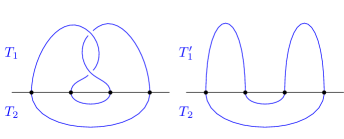
Figure 17. Two non-ambient isotopic tangles $T_{1}\not\simeq T_{1}^{\prime}$ such that $T_{1}\#T_{2}\simeq T_{1}^{\prime}\#T_{2}$.

Lemma 3.32.

$KCH^{\ast}_{\mathrm{EENS}}(K)$ detects the $r$-component unlink up to ambient isotopy and mirroring for any $r\geq 1$.

Proof.

This is already known in the case $r=1$ by [CELN17, Proposition 2.19]. The same argument as in [CELN17, Proposition 2.21] and [CELN17, Proof of Corollary 1.5] (cf. [GL17, Remark 5]) can be used for $r>1$, which we recall below.

By [CELN17, Theorem 1.2 and Proposition 2.21] we have that

(3.3) $$KCH^{0}_{\text{EENS}}(K)\cong\mathfrak{R}$$

for framed oriented non-trivial knots in ${\mathbb{R}}^{3}$. Here $\mathfrak{R}$ is defined as the subring of ${\mathbb{Z}}[\pi_{1}({\mathbb{R}}^{3}\setminus K)]$ generated by $\pi_{1}(\lambda_{1}^{\pm 1},\mu_{1}^{\pm 1},\ldots,\lambda_{r}^{\pm 1},\mu_{r}^{\pm 1})$, and $\operatorname{im}(1-\mu_{i})$ for $i\in\left\{1,\ldots,r\right\}$ where $1-\mu_{i}$ denotes the map ${\mathbb{Z}}[\pi_{1}({\mathbb{R}}^{3}\setminus K)]\longrightarrow{\mathbb{Z}}[\pi_{1}({\mathbb{R}}^{3}\setminus K)]$ given by left multiplication by $1-\mu_{i}$. We claim that (3.3) still holds for framed oriented $r$-component non-trivial links using the same argument as in [CELN17, Proof of Proposition 2.21].

By [HS85, Lemma 2] we have that $\pi_{1}({\mathbb{R}}^{3}\setminus K)$ is locally indicable and hence ${\mathbb{Z}}[\pi_{1}({\mathbb{R}}^{3}\setminus K)]$ is an integral domain by [Hig40, Theorem 12]. By computation we have that

$$KCH^{0}_{\text{EENS}}(U)\cong{\mathbb{Z}}[\pi_{1}(\lambda_{1}^{\pm 1},\mu_{1}^{\pm 1},\ldots,\lambda_{r}^{\pm 1},\mu_{r}^{\pm 1})]/\left\langle((1-\lambda_{i})(1-\mu_{i})\;|\;i\in\left\{1,\ldots,r\right\}\right\rangle$$

(see [EENS13]) which is not an integral domain, and thus $KCH^{\ast}_{\text{EENS}}(K)\not\cong KCH^{\ast}_{\text{EENS}}(U)$. ∎

Lemma 3.33.

Let $T,T^{\prime}\subset{\mathbb{R}}^{3}_{x\geq 0}$ be two tangles. Assume that $\overline{\mathcal{G}}_{T\to H}\cong\overline{\mathcal{G}}_{T^{\prime}\to H}$ and $\overline{\mathcal{G}}_{H\to T}\cong\overline{\mathcal{G}}_{H\to T^{\prime}}$ as right and left modules over $\mathcal{G}_{H}$, respectively. Then if there is a quasi-isomorphism of dg-algebras $KCC^{\ast}(T,h)\cong KCC^{\ast}(T^{\prime},h^{\prime})$ we have a quasi-isomorphism

$$KCC^{\ast}(T\#T^{\prime\prime},h\#h^{\prime\prime})\cong KCC^{\ast}(T^{\prime}\#T^{\prime\prime},h^{\prime}\#h^{\prime\prime}).$$

Proof.

This follows from the definition (3.2). Indeed, if $\overline{\mathcal{G}}_{T\to H}\cong\overline{\mathcal{G}}_{T^{\prime}\to H}$ and $\overline{\mathcal{G}}_{H\to T}\cong\overline{\mathcal{G}}_{H\to T^{\prime}}$ as right and left modules over $\mathcal{G}_{H}$, respectively, then it follows that

$$\mathcal{G}_{T\to H\to T^{\prime\prime}}\cong\mathcal{G}_{T^{\prime}\to H\to T^{\prime\prime}},\qquad\mathcal{G}_{T^{\prime\prime}\to H\to T}\cong\mathcal{G}_{T^{\prime\prime}\to H\to T^{\prime}}$$

from which the conclusion holds by 3.28. ∎

Definition 3.34 (Weak detection).

We say that tangle contact homology weakly detects a tangle $T\subset{\mathbb{R}}^{3}_{x\geq 0}$ if for any tangle $T^{\prime}$ that satisfies $\mathcal{G}_{T\to H}\cong\mathcal{G}_{T^{\prime}\to H}$ and $\mathcal{G}_{H\to T}\cong\mathcal{G}_{H\to T^{\prime}}$ as right and left modules over $\mathcal{G}_{H}$, respectively, we have that $KCC^{\ast}(T,h)\cong KCC^{\ast}(T^{\prime},h^{\prime})$ implies $T\simeq T^{\prime}$.

Theorem 3.35.

Let $T\subset{\mathbb{R}}^{3}_{x\geq 0}$ be a tangle and let $h$ be one of the handle decompositions $h_{1}$ and $h_{2}$ of $N(\varLambda_{T})$ from Section 3.4.1. The tangle contact homology of $T$ weakly detects the $r$-component untangle.

Proof.

Let $K=T_{1}\#T_{2}$ be a splitting of the $r$-component unlink into two trivial $r$-component tangles. Let $T_{1}^{\prime}$ be any $r$-component tangle which is not ambient isotopic to $T_{1}$ and so that it satisfies $\mathcal{G}_{T_{1}\to H}\cong\mathcal{G}_{T_{1}^{\prime}\to H}$ and $\mathcal{G}_{H\to T_{1}}\cong\mathcal{G}_{H\to T_{1}^{\prime}}$ as right and left modules over $\mathcal{G}_{H}$, respectively. Then by 3.30 it follows that $K^{\prime}\mathrel{\mathop{\mathchar 58\relax}}=T_{1}^{\prime}\#T_{2}$ is a non-trivial $r$-component link. Let $h_{1}$ and $h_{2}$ be the two handle decompositions as in Section 3.4.1. By 3.32 we thus have $KCH^{\ast}_{\text{EENS}}(K)\not\cong KCH^{\ast}_{\text{EENS}}(K^{\prime})$. It then follows from 3.33 that $KCC^{\ast}(T_{1},h_{1})\not\cong KCC^{\ast}(T_{1}^{\prime},h_{1})$. ∎

Example 3.36.

Figure 18. A tangle given by the half-closure of a braid $\beta$. The two vertical red lines on the right are binormal geodesics corresponding to the generators of $\mathcal{G}_{T_{\beta}\to H}$ and $\mathcal{G}_{H\to T_{\beta}}$, respectively.

To illustrate the definition of weak detection in 3.34, we consider the tangle $T_{\beta}$ as shown in Figure 18. We have that 3.35 in particular shows that $KCC^{\ast}(T_{\beta},h_{1})$ detects the untangle among the tangles $T_{\beta}$. This is because we can do crossing changes to pass from $T_{\beta}$ to $T_{\beta}^{\prime}$ which is not ambient isotopic to $T_{\beta}$. We may assume that the strands of $T_{\beta}$ are arranged so that $\mathcal{G}_{T_{\beta}\to H}$ and $\mathcal{G}_{H\to T_{\beta}}$ are both generated by one oriented binormal geodesic per strand in ${\mathbb{R}}^{3}_{x\geq 0}$, see Figure 18. After changing a crossing in the braid, the same remains true and so we have $\mathcal{G}_{T_{\beta}\to H}\cong\mathcal{G}_{T_{\beta}^{\prime}\to H}$ and $\mathcal{G}_{H\to T_{\beta}}\cong\mathcal{G}_{H\to T_{\beta}^{\prime}}$ as right and left modules over $\mathcal{G}_{\partial H}$, respectively.

Definition 3.37 (Ambient isotopy with moving boundary).

We say that two tangles $T_{1}$ and $T_{2}$ in ${\mathbb{R}}^{3}_{x\geq 0}$ are ambient isotopic with moving boundary if there is an isotopy $h_{t}\colon{\mathbb{R}}^{3}_{x\geq 0}\longrightarrow{\mathbb{R}}^{3}_{x\geq 0}$ such that items (1) and (2) (but not necessarily item (3)) in 3.3 holds.

Corollary 3.38.

The quasi-isomorphism class of $KCC^{\ast}(T,h)$ is not invariant under ambient isotopies with moving boundary of $T$.

Proof.

This follows the proof of 3.35 by choosing $T_{1}^{\prime}$ to be a tangle which is not ambient isotopic to $T_{1}$ but ambient isotopic with moving boundary. We may for instance take $T_{1}$ and $T_{1}^{\prime}$ as shown in Figure 17. ∎

4. Examples

Example 4.1 (Unframed subalgebra).

Let us first consider a single stranded braid $T\subset{\mathbb{R}}^{3}_{x\geq 0}$. Its boundary is two points in $\partial{\mathbb{R}}^{3}_{x\geq 0}\cong{\mathbb{R}}^{2}$. The unframed knot contact homology $KCC^{\ast}_{u}(\partial T)$ is simply the knot contact homology (without homology coefficients) of two points $z_{1},z_{2}\in{\mathbb{R}}^{2}$. As $KCC^{\ast}_{u}(\partial T)$ is generated by oriented binormal geodesics, we know that there are two generators $c_{1}$ and $c_{2}$, both in degree $0$. Their differentials are also trivial. Hence $KCC^{\ast}_{u}(\partial T)\cong\boldsymbol{k}[c_{1},c_{2}]$. Computing the degree and differential is done using the front projection of $\varLambda_{z_{1}},\varLambda_{z_{2}}\subset ST^{\ast}{\mathbb{R}}^{2}\cong J^{1}(S^{1})$, which lie in $S^{1}\times{\mathbb{R}}\cong{\mathbb{R}}^{2}\setminus\left\{0\right\}$, see Figure 19.

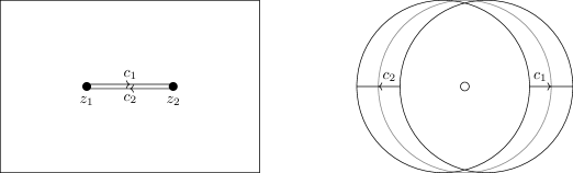
Figure 19. Left: The two oriented binormal geodesics of $\partial T\subset{\mathbb{R}}^{2}$. Right: The two front projections of $\varLambda_{z_{1}}$ and $\varLambda_{z_{2}}$ in $S^{1}\times{\mathbb{R}}\cong{\mathbb{R}}^{2}\setminus\left\{0\right\}$ with the two Reeb chords $c_{1}$ and $c_{2}$ drawn. The front projection of the zero section of $J^{1}(S^{1})$ is the central gray circle.

We now give a surgery presentation of $KCC^{\ast}_{u}(\partial T)$. Namely, present $T^{\ast}{\mathbb{R}}^{2}$ as $B^{4}$ stopped at the standard unknot $\varLambda_{\text{unknot}}\subset S^{3}=\partial B^{4}$, see also [AE22, Example 7.4]. This means that we present $T^{\ast}{\mathbb{R}}^{2}$ as the result of attaching a copy of $T^{\ast}(\varLambda_{\text{unknot}}\times{\mathbb{R}}_{\geq 0})$ to $B^{4}$ along a cotangent neighborhood of $\varLambda_{\text{unknot}}$, see Figure 20.

Figure 20. Surgery presentation of the open Weinstein sector $T^{\ast}{\mathbb{R}}^{2}$ as $B^{4}$ stopped at the standard unknot in $S^{3}$.

Now, we can use surgery techniques to give a quasi-isomorphic presentation of $KCC^{\ast}_{u}(\partial T)$ which is more amenable to proving the gluing formulas in this paper. Namely, removing the cotangent bundle $T^{\ast}(\varLambda_{\text{unknot}}\times{\mathbb{R}}_{\geq 0})$, we are left with the Legendrians $\varLambda_{z_{1}},\varLambda_{z_{2}},\varLambda_{\text{unknot}}\subset S^{3}=\partial B^{4}$. By the same technique used to prove [BEE12, Theorem 5.10] and [Ekh19, Theorem 1.2] we have that $KCC^{\ast}_{u}(\partial T)$ is quasi-isomorphic to the dg-algebra generated by composable words of Reeb chords of the form

(4.1) $$\varLambda_{z_{i}}\to\overline{\varLambda}_{\text{unknot}}\to\cdots\to\overline{\varLambda}_{\text{unknot}}\to\varLambda_{z_{j}},$$

for $i,j\in\left\{1,2\right\}$ where $\overline{\varLambda}_{\text{unknot}}$ is a Legendrian submanifold in the positive boundary of the Weinstein cobordism obtained by attaching a handle $(B^{2}\times D_{\varepsilon}T^{\ast}[0,1],\frac{1}{2}(qdp-pdq)+2xdy+ydx)$ to $B^{4}\sqcup((-\infty,0]\times B^{2}\times{\mathbb{R}})$, see [AE22, Section 1.2] for a general description. The Legendrian $\overline{\varLambda}_{\text{unknot}}$ is now defined in the same way as $\varSigma(h)$ in [AE22, Equation (1.1)]. This is geometrically saying that we consider loop space coefficients in the component $\varLambda_{\text{unknot}}$ only. The differential used in the dg-algebra generated by words of the form as in (4.1) is induced by the differential of the Chekanov–Eliashberg dg-algebra of the Legendrian link $\varLambda_{z_{1}}\cup\varLambda_{z_{2}}\cup\overline{\varLambda}_{\text{unknot}}\subset\partial B^{4}_{T^{\ast}D^{2}}$. After a Legendrian isotopy this link fits in a Darboux chart and the front projection in ${\mathbb{R}}^{2}$ is shown in Figure 21.

Figure 21. The front projection of the Legendrian link $\varLambda_{z_{1}}\cup\varLambda_{z_{2}}\cup\ell_{\text{unknot}}$ in a Darboux chart.

The Legendrian $\overline{\varLambda}_{\text{unknot}}$ consists of a $1$-dimensional disk $\ell_{\text{unknot}}$ with boundary $\partial\ell_{\text{unknot}}\subset B^{2}$ where $B^{2}$ is the subcritical part after a choice of handle decomposition of a Weinstein neighborhood of $\varLambda_{\text{unknot}}$. It follows from [AE22, Lemma 3.4] that Reeb chords of $\overline{\varLambda}_{\text{unknot}}$ corresponds to Reeb chords of $\ell_{\text{unknot}}$ that are contained in $S^{3}$ (this is the Reeb chord labeled by $a$ in Figure 21) and Reeb chords of $\partial\ell_{\text{unknot}}\subset B^{2}$. The Reeb chords of the latter kind corresponds to Reeb chords of two points in the boundary of $B^{2}$, and they form a dg-subalgebra described in detail in [EN15, Section 2.3], see also [AE22, Example 7.3] and references therein. With appropriate choices of Maslov potential, the two shortest Reeb chords corresponding to the point $t$ in Figure 21 are denoted by $t^{0}_{12}$ and $t^{1}_{21}$ using the notation as in [AE22, Example 7.3].

Inside this Darboux chart there are two Reeb chords between $\varLambda_{z_{1}}$ and $\varLambda_{\text{unknot}}$ and also two Reeb chords between $\varLambda_{z_{2}}$ and $\varLambda_{\text{unknot}}$, labeled in Figure 21 by $q_{1},p_{1}$ and $q_{2},p_{2}$, respectively. Note that since this Legendrian link is in $S^{3}$, there are in general more Reeb chords that necessarily leaves the Darboux chart. Using [EN15, Lemma 4.6] and an action argument like the proof of [EN15, Lemma 5.6] we obtain that $KCC^{\ast}_{u}(\partial T)$ is quasi-isomorphic to the dg-algebra generated by composable words formed by products of the following two kinds:

1. $a_{1}$ and $a_{2}$ both in degree $1$.

2. The words $q_{j}c^{k}p_{i}$ for $k\geq 0$, $i,j\in\left\{1,2\right\}$, where $c$ is any Reeb chord $\overline{\varLambda}_{\text{unknot}}$, of degree $|c|$.

The differential is induced by the differential of the Chekanov–Eliashberg dg-algebra of $\varLambda_{z_{1}}\cup\varLambda_{z_{2}}\cup\overline{\varLambda}_{\text{unknot}}$ which can be computed from Figure 21 to be as follows with coefficients in ${\mathbb{Z}}_{2}$

$$\begin{cases}\partial a_{1}=p_{1}q_{1}\\ \partial a_{2}=p_{2}q_{2}\\ \partial a=e_{\text{unknot}}+t^{0}_{12}+q_{1}p_{1}+q_{2}p_{2}\\ \partial q_{i}=\partial p_{i}=0\end{cases},$$

where $e_{\text{unknot}}$ denotes the idempotent corresponding to the component $\overline{\varLambda}_{\text{unknot}}$. By the general theory the just described dg-algebra is quasi-isomorphic to $KCC^{\ast}_{u}(\partial T)$ although we do not attempt to exhibit an explicit such quasi-isomorphism.

Example 4.2 (Framed subalgebra).

We upgrade 4.1 and now compute $KCC^{\ast}(\partial T,h_{\partial})$. The difference is now that we pick a handle decomposition $h_{\partial}$ of a chosen Weinstein neighborhood $N(\varLambda_{\partial T})=N(\varLambda_{z_{1}})\cup N(\varLambda_{z_{2}})$. We construct $\overline{\varLambda}_{z_{i}}$ for $i\in\left\{1,2\right\}$ in the same way as $\overline{\varLambda}_{\text{unknot}}$ in 4.1. Computationally, we have two more infinite families of Reeb chords to take into account, indicated by the two points $t(1)$ and $t(2)$, see Figure 22.

Figure 22. The front projection of the Legendrian link $\overline{\varLambda}_{z_{1}}\cup\overline{\varLambda}_{z_{2}}\cup\ell_{\text{unknot}}$ in a Darboux chart.

By the general theory we now have that the dg-algebra $KCC^{\ast}(\partial T)$ is quasi-isomorphic to the dg-algebra generated by composable words formed by products of the following two kinds:

1. $a_{1}$ and $a_{2}$ both in degree $1$

2. Reeb chords $t(1)^{p}_{ij}$ and $t(2)^{p}_{ij}$ with notation as in [AE22, Example 7.3].

3. The words $q_{j}c^{k}p_{i}$ for $k\geq 0$, $i,j\in\left\{1,2\right\}$, where $c$ is any Reeb chord $\overline{\varLambda}_{\text{unknot}}$, of degree $|c|$.

The differential is induced by the differential of the Chekanov–Eliashberg dg-algebra of $\overline{\varLambda}_{z_{1}}\cup\overline{\varLambda}_{z_{2}}\cup\overline{\varLambda}_{\text{unknot}}$ which can be computed from Figure 22 to be as follows with coefficients in ${\mathbb{Z}}_{2}$

$$\begin{cases}\partial a_{1}=e_{1}+t(1)^{0}_{12}+p_{1}q_{1}\\ \partial a_{2}=e_{2}+t(2)^{0}_{12}+p_{2}q_{2}\\ \partial a=e_{\text{unknot}}+t^{0}_{12}+q_{1}p_{1}+q_{2}p_{2}\\ \partial q_{i}=\partial p_{i}=0\end{cases},$$

where $e_{i}$ and $e_{\text{unknot}}$ denotes the idempotent corresponding to the components $\overline{\varLambda}_{z_{i}}$ and $\overline{\varLambda}_{\text{unknot}}$, respectively for $i\in\left\{1,2\right\}$.

Above and in 4.1 we have used a description of $KCC^{\ast}(\partial T,h_{\partial})$ which only uses Reeb chords of the front projecting appearing in the Darboux chart. Instead, we consider $\overline{\varLambda}_{\text{unknot}}$ and $\overline{\varLambda_{z_{i}}}$ before applying the Legendrian isotopy to make them fit in a Darboux chart. Namely, the Reeb chords of the link $\overline{\varLambda}_{z_{1}}\cup\overline{\varLambda}_{z_{2}}\cup\overline{\varLambda}_{\text{unknot}}$ come in two families of $S^{1}$-families, one corresponding to Reeb chords of $\overline{\varLambda}_{z_{1}}\cup\overline{\varLambda}_{\text{unknot}}$ and one corresponding to Reeb chords of $\overline{\varLambda}_{z_{2}}\cup\overline{\varLambda}_{\text{unknot}}$. After Morsification, the shortest Reeb chords are as indicated in the following diagram.

(4.2)

The differential (with coefficients in ${\mathbb{Z}}_{2}$) is given by the following.

$$\begin{cases}\partial q_{1}=\partial q_{2}=\partial p_{1}=\partial p_{2}=0\\ \partial\widehat{q}_{1}=q_{1}+t^{0}_{12}q_{1}\\ \partial\widehat{q}_{2}=q_{2}+t^{0}_{12}q_{2}\\ \partial\widehat{p}_{1}=p_{1}+p_{1}t^{0}_{12}\\ \partial\widehat{p}_{2}=p_{2}+p_{2}t^{0}_{12}\\ \partial a=e_{\text{unknot}}+t^{0}_{12}+q_{1}p_{1}+q_{2}p_{2}\\ \partial a_{1}=e_{1}+t(1)^{0}_{12}+p_{1}q_{1}\\ \partial a_{2}=e_{2}+t(2)^{0}_{12}+p_{2}q_{2}\end{cases}.$$

Example 4.3 (Unframed trivial tangle).

Let us now consider $T\subset{\mathbb{R}}^{3}_{x\geq 0}$ the trivial tangle as depicted in Figure 23. The hypersurface $H$ is the graph of the function $f(x,y)=x^{2}-y^{2}$ with a saddle point at the origin.

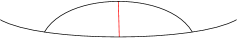
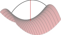
Figure 23. The trivial tangle in ${\mathbb{R}}^{3}_{x\geq 0}$. The vertical red line is the only unoriented binormal geodesic chord between $T$ and $H$.

By 3.21 we know that $KCC^{\ast}_{u}(T)$ is quasi-isomorphic to the dg-algebra generated by oriented binormal geodesic chords between $T$ and $H$, since there are no binormal geodesic chords of $T$ and none of $H$. We also know that $KCC^{\ast}_{u}(\partial T)\subset KCC^{\ast}_{u}(T)$ is a dg-subalgebra that we have already described in 4.1. The degree of both of the two Reeb chords $c_{T\to H}$ and $c_{H\to T}$ is $1$. The differential is given by

(4.3) $$\begin{cases}\partial c_{T\to H}=q_{1}+q_{2}\\ \partial c_{H\to T}=p_{1}+p_{2}\end{cases}$$

For each Reeb chord, the two $J$-holomorphic disks may be visualized in Figure 23 by imagining that the oriented binormal geodesic chord moving right or left and shrinks down to a point.

Example 4.4 (Framed trivial tangle).

Let us now consider $T\subset{\mathbb{R}}^{3}_{x\geq 0}$ the trivial tangle, see Figure 23. We let $h_{1}$ and $h_{2}$ be the handle decomposition of $N(\varLambda_{T})$ as depicted in Figure 15 and Figure 16, respectively. The subalgebra $KCC^{\ast}(\partial T,h_{\partial})$ is as described in 4.2.

We first consider $KCC^{\ast}(T,h_{2})$. There is one additional set of generators corresponding to $\mathinner{\partial\ell_{T}\rvert}_{V_{T}}$, see Figure 14. This set of generators is denoted by $\left\{\widehat{t}^{p}_{ij}\right\}$ and should be interpreted as follows. In $V_{T}$ there is a one-parameter family of dg-algebras all of which is quasi-isomorphic to the Chekanov–Eliashberg dg-algebra of two distinct points in $S^{1}$. After Morsification by a function with a maximum in the interior and two minima at the boundary of $\varLambda_{T}$. The generators $\left\{\widehat{t}^{p}_{ij}\right\}$ correspond to the maximum and $\left\{t(i)^{p}_{ij}\right\}$ correspond to the two minima; they are depicted in Figure 24. Together $\left\{\widehat{t}^{p}_{ij},t(1)^{p}_{ij},t(2)^{p}_{ij}\right\}$ generate a dg-algebra that is quasi-isomorphic to $CE^{\ast}(\mathinner{\partial\ell_{T}\rvert}_{V_{T}},Q_{T};V_{T})$, see Figure 22 and Figure 24.

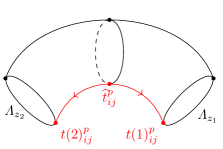
Figure 24. A sketch of the generators of $CE^{\ast}(\mathinner{\partial\ell\rvert}_{V_{T}},Q_{T};V_{T})$ and their differential, using the handle decomposition $h_{2}$.

The differential of $\widehat{t}^{p}_{ij}$ is given by

(4.4) $$\partial\widehat{t}^{p}_{ij}=t(1)^{p}_{ij}+t(2)^{p}_{ij}+G(\partial\widehat{t}^{p}_{ij}).$$

where $G$ is defined as follows on monomials

$$G(\widehat{t}^{p_{1}}_{i_{1}j_{1}}\widehat{t}^{p_{2}}_{i_{2}j_{2}}\cdots\widehat{t}^{p_{m}}_{i_{m}j_{m}}) =\widehat{t}^{p_{1}}_{i_{1}j_{1}}t(2)^{p_{2}}_{i_{2}j_{2}}\cdots t(2)^{p_{m}}_{i_{m}j_{m}}+t(1)^{p_{1}}_{i_{1}j_{1}}\widehat{t}^{p_{2}}_{i_{2}j_{2}}\cdots\widehat{t}(2)^{p_{m}}_{i_{m}j_{m}}$$

$$\quad+\cdots t(1)^{p_{1}}_{i_{1}j_{1}}t(1)^{p_{2}}_{i_{2}j_{2}}\cdots\widehat{t}^{p_{m}}_{i_{m}j_{m}},$$

and extended to the whole algebra by linearity [EK08, Corollary 5.6].

As in 4.3 we have two unoriented binormal geodesic chords $c_{T\to H}$ and $c_{H\to T}$ corresponding to generators of $KCC^{\ast}(T,h_{2})$ of degree $1$. Their differential is given by the same formula as in the unframed case, namely as in (4.3).

Similar to the above we now describe $KCC^{\ast}(T,h_{1})$. The dg-algebra $CE^{\ast}(\mathinner{\partial\ell\rvert}_{V_{T}},Q_{T};V_{T})$ is now more complicated and we do not fully describe it. We remark however that if setting $t(1)^{p}_{ij}=t(2)^{p}_{ij}$, it is quasi-isomorphic to the one exhibited in [EN15, Section 2.5] which is the Chekanov–Eliashberg dg-algebra of the top attaching sphere of $T^{\ast}T^{2}$ equipped with its standard handle decomposition consisting of one $0$-handle, two $1$-handles and one $2$-handle.

Furthermore, there is a certain dg-subalgebra of $CE^{\ast}(\mathinner{\partial\ell\rvert}_{V_{T}},Q_{T};V_{T})$ that is generated by $\left\{c^{p}_{ij}\right\}$ which again is quasi-isomorphic to the Chekanov–Eliashberg dg-algebra of two points in $S^{1}$, see Figure 25

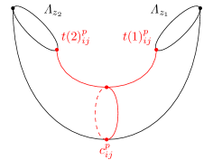
Figure 25. A sketch of some of the generators of $CE^{\ast}(\mathinner{\partial\ell\rvert}_{V_{T}},Q_{T};V_{T})$ using the handle decomposition $h_{1}$.

As above we have two unoriented binormal geodesic chords $c_{T\to H}$ and $c_{H\to T}$ corresponding to generators of $KCC^{\ast}(T,h_{1})$ of degree $1$. Their differential is given by the following.

$$\begin{cases}\partial c_{T\to H}=q_{1}+q_{2}c^{0}_{12}\\ \partial c_{H\to T}=p_{1}+c^{1}_{21}p_{2}\end{cases}$$

Example 4.5 (Unknot).

Let $K\subset{\mathbb{R}}^{3}$ be the unknot. First split $K$ into the gluing with $H$ that is (an affine transformation of) the graph of $f(x,y)=x^{2}-y^{2}$ of two tangles as shown in Figure 26 and Figure 27.

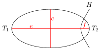
Figure 26. The unknot obtained by gluing of the two tangles $T_{1}$ and $T_{2}$.

Figure 27. Left: A side view of the tangle $T_{2}$. Right: A side view of the tangle $T_{1}$ revealing two extra binormal geodesic chords $a$ and $a^{\prime}$.

Let $h_{1}$ be the handle decomposition of $N(\varLambda_{T_{1}})$ depicted in Figure 16 and let $h_{2}$ be the handle decomposition of $N(\varLambda_{T_{2}})$ depicted in Figure 15. We already computed $KCC^{\ast}(T_{2},h_{2})$ in 4.4 so we will focus on $KCC^{\ast}(T_{1},h_{1})$. From Figure 26 we see that we have two unoriented binormal geodesic chords $c$ and $e$ corresponding to Reeb chords $c_{1}$, $c_{2}$, $e_{T_{1}\to H}$, $e_{H\to T_{1}}$, where $|c|=1$ and $|e|=2$. Furthermore we have that Figure 27 reveals two more unoriented binormal geodesic chords $a$ and $a^{\prime}$ with $|a|=|a^{\prime}|=1$. The differentials are given by (with coefficients in ${\mathbb{Z}}_{2}$) the following.

$$\begin{cases}\partial a_{T_{1}\to H}=q_{1}t(1)^{0}_{12}+q_{2}t(2)^{0}_{12}\\ \partial a_{H\to T_{1}}=t(1)^{0}_{12}p_{1}+t(2)^{0}_{12}p_{2}\\ \partial a^{\prime}_{T_{1}\to H}=q_{1}t(1)^{1}_{21}+q_{2}t(2)^{1}_{21}\\ \partial a^{\prime}_{H\to T_{1}}=t(1)^{1}_{21}p_{1}+t(2)^{1}_{21}p_{2}\\ \partial c_{1}=e_{1}+t(2)^{1}_{21}+p_{1}q_{2}\\ \partial c_{2}=e_{2}+t(1)^{1}_{21}+p_{2}q_{1}\\ \partial e_{T_{1}\to H}=q_{1}(c_{1}+a_{1})+q_{2}(c_{2}+a_{2})+a(q_{1}+q_{2})+\widehat{q}_{1}+\widehat{q}_{2}+a_{T_{1}\to H}+a^{\prime}_{T_{1}\to H}\\ \partial e_{H\to T_{1}}=(c_{2}+a_{1})p_{1}+(c_{1}+a_{2})p_{2}+(p_{1}+p_{2})a+\widehat{p}_{1}+\widehat{p}_{2}+a_{H\to T_{1}}+a^{\prime}_{H\to T_{1}}\\ \end{cases}.$$

References

- [Abo12] Mohammed Abouzaid. On the wrapped Fukaya category and based loops. J. Symplectic Geom., 10(1):27–79, 2012.
- [AE22] Johan Asplund and Tobias Ekholm. Chekanov–Eliashberg dg-algebras for singular Legendrians. J. Symplectic Geom., 20(3):509–559, 2022.
- [ÁGEN22] Daniel Álvarez-Gavela, Yakov Eliashberg, and David Nadler. Positive arborealization of polarized Weinstein manifolds. arXiv:2011.08962, 2022.
- [Asp21] Johan Asplund. Fiber Floer cohomology and conormal stops. J. Symplectic Geom., 19(4):777–864, 2021.
- [Asp23] Johan Asplund. Simplicial descent for Chekanov-Eliashberg dg-algebras. J. Topol., 16(2):489–541, 2023.
- [Avd21] Russell Avdek. Liouville hypersurfaces and connect sum cobordisms. J. Symplectic Geom., 19(4):865–957, 2021.
- [BEE12] Frédéric Bourgeois, Tobias Ekholm, and Yasha Eliashberg. Effect of Legendrian surgery. Geom. Topol., 16(1):301–389, 2012. With an appendix by Sheel Ganatra and Maksim Maydanskiy.
- [BNR16] Maciej Borodzik, András Némethi, and Andrew Ranicki. Morse theory for manifolds with boundary. Algebr. Geom. Topol., 16(2):971–1023, 2016.
- [CDRGG17] Baptiste Chantraine, Georgios Dimitroglou Rizell, Paolo Ghiggini, and Roman Golovko. Geometric generation of the wrapped Fukaya category of Weinstein manifolds and sectors. arXiv:1712.09126, 2017.
- [CELN17] Kai Cieliebak, Tobias Ekholm, Janko Latschev, and Lenhard Ng. Knot contact homology, string topology, and the cord algebra. J. Éc. polytech. Math., 4:661–780, 2017.
- [Che02] Yuri Chekanov. Differential algebra of Legendrian links. Invent. Math., 150(3):441–483, 2002.
- [Dat] Côme Dattin. Sutured Legendrian stops and the conormal of surface braids. In preparation.
- [Dat22] Côme Dattin. Wrapped sutured Legendrian homology and unit conormal of local 2-braids. arXiv:2206.11582, 2022.
- [DR16] Georgios Dimitroglou Rizell. Lifting pseudo-holomorphic polygons to the symplectisation of and applications. Quantum Topol., 7(1):29–105, 2016.
- [EENS13] Tobias Ekholm, John B. Etnyre, Lenhard Ng, and Michael G. Sullivan. Knot contact homology. Geom. Topol., 17(2):975–1112, 2013.
- [EES05] Tobias Ekholm, John Etnyre, and Michael Sullivan. The contact homology of Legendrian submanifolds in . J. Differential Geom., 71(2):177–305, 2005.
- [EES07] Tobias Ekholm, John Etnyre, and Michael Sullivan. Legendrian contact homology in . Trans. Amer. Math. Soc., 359(7):3301–3335, 2007.
- [EGH00] Y. Eliashberg, A. Givental, and H. Hofer. Introduction to symplectic field theory. Number Special Volume, Part II, pages 560–673. 2000. GAFA 2000 (Tel Aviv, 1999).
- [EK08] Tobias Ekholm and Tamás Kálmán. Isotopies of Legendrian 1-knots and Legendrian 2-tori. J. Symplectic Geom., 6(4):407–460, 2008.
- [Ekh18] Tobias Ekholm. Knot contact homology and open Gromov-Witten theory. In Proceedings of the International Congress of Mathematicians—Rio de Janeiro 2018. Vol. II. Invited lectures, pages 1063–1086. World Sci. Publ., Hackensack, NJ, 2018.
- [Ekh19] Tobias Ekholm. Holomorphic curves for Legendrian surgery. arXiv:1906.07228, 2019.
- [EL17] Tobias Ekholm and Yankı Lekili. Duality between Lagrangian and Legendrian invariants. arXiv:1701.01284, 2017.
- [Eli98] Yakov Eliashberg. Invariants in contact topology. In Proceedings of the International Congress of Mathematicians, Vol. II (Berlin, 1998), number Extra Vol. II, pages 327–338, 1998.
- [Eli18] Yakov Eliashberg. Weinstein manifolds revisited. In Modern geometry: a celebration of the work of Simon Donaldson, volume 99 of Proc. Sympos. Pure Math., pages 59–82. Amer. Math. Soc., Providence, RI, 2018.
- [EN15] Tobias Ekholm and Lenhard Ng. Legendrian contact homology in the boundary of a subcritical Weinstein 4-manifold. J. Differential Geom., 101(1):67–157, 2015.
- [ENS18] Tobias Ekholm, Lenhard Ng, and Vivek Shende. A complete knot invariant from contact homology. Invent. Math., 211(3):1149–1200, 2018.
- [EO17] Tobias Ekholm and Alexandru Oancea. Symplectic and contact differential graded algebras. Geom. Topol., 21(4):2161–2230, 2017.
- [GL17] Cameron Gordon and Tye Lidman. Knot contact homology detects cabled, composite, and torus knots. Proc. Amer. Math. Soc., 145(12):5405–5412, 2017.
- [GPS20] Sheel Ganatra, John Pardon, and Vivek Shende. Covariantly functorial wrapped Floer theory on Liouville sectors. Publ. Math. Inst. Hautes Études Sci., 131:73–200, 2020.
- [GPS22] Sheel Ganatra, John Pardon, and Vivek Shende. Sectorial descent for wrapped Fukaya categories. arXiv:1809.03427v3, 2022.
- [Hig40] Graham Higman. The units of group-rings. Proc. London Math. Soc. (2), 46:231–248, 1940.
- [HS85] James Howie and Hamish Short. The band-sum problem. J. London Math. Soc. (2), 31(3):571–576, 1985.
- [Kar20] Cecilia Karlsson. Legendrian contact homology for attaching links in higher dimensional subcritical Weinstein manifolds. arXiv:2007.07108, 2020.
- [KM07] Peter Kronheimer and Tomasz Mrowka. Monopoles and three-manifolds, volume 10 of New Mathematical Monographs. Cambridge University Press, Cambridge, 2007.
- [Ng05a] Lenhard Ng. Knot and braid invariants from contact homology. I. Geom. Topol., 9:247–297, 2005.
- [Ng05b] Lenhard Ng. Knot and braid invariants from contact homology. II. Geom. Topol., 9:1603–1637, 2005. With an appendix by the author and Siddhartha Gadgil.
- [Ng08] Lenhard Ng. Framed knot contact homology. Duke Math. J., 141(2):365–406, 2008.
- [Ng14] Lenhard Ng. A topological introduction to knot contact homology. In Contact and symplectic topology, volume 26 of Bolyai Soc. Math. Stud., pages 485–530. János Bolyai Math. Soc., Budapest, 2014.