Interplay of Pauli blockade with electron-photon coupling in quantum dots

Abstract

Both quantum transport measurements in the Pauli blockade regime and microwave cavity transmission measurements are important tools for spin-qubit readout and characterization. Based on a generalized input-output theory we derive a theoretical framework to investigate how a double quantum dot (DQD) in a transport setup interacts with a coupled microwave resonator while the current through the DQD is rectified by Pauli blockade. We show that the output field of the resonator can be used to infer the leakage current and thus obtain insight into the blockade mechanisms. In the case of a silicon DQD, we show how the valley quasi-degeneracy can impose limitations on this scheme. We also demonstrate that a large number of unknown DQD parameters including (but not limited to) the valley splitting can be estimated from the resonator response simultaneous to a transport experiment, providing more detailed knowledge about the microscopic environment of the DQD. Furthermore, we describe and quantify a back-action of the resonator photons on the steady state leakage current.

I Introduction

Spin qubits in few-electron quantum dots (QDs) [1] are advancing to become one of the leading platforms for quantum information, with numerous demonstrations of high-fidelity quantum operations on the few-qubit scale [2, 3, 4, 5]. Great hopes to achieve the required scalability lie with circuit quantum electrodynamics (cQED) implementations [6], relying on the dipole moment of electrons in a double QD (DQD). After strong spin-photon coupling [7, 8, 9, 10] and cavity-mediated spin-spin coupling [11, 12] have been demonstrated, photon-mediated two-qubits gates [13, 14, 15, 16] and resonator-based spin readout [17, 18, 19, 20, 21, 22, 23] are conceivable.

Another well established instrument in the spin qubit-toolbox is Pauli blockade [24, 1]. A DQD with two electrons can be in a state with one electron in each dot or one doubly occupied QD. Due to the Pauli exclusion principle not all two-electron states are allowed in a doubly occupied QD. For example, two electrons forming a spin triplet in two dots cannot be merged into one QD unless the excited orbital state becomes available [25]. In a closed system the Pauli blockade can be harnessed for initialization [26, 27, 28] and readout [26, 29] of different types of spin qubits.

In a transport setup Pauli blockade can lead to a rectification of the current through a DQD already occupied with one electron [30]. The blockade can be partially lifted by interactions that mix the spin states such as spin-orbit interaction [31, 32], hyperfine interaction [33, 34, 35] or cotunneling processes [36, 37]. The observation of Pauli blockade is proof of a large single-dot singlet-triplet splitting and therefore a crucial first step towards spin qubit applications.

If the DQD is driven by AC fields the characteristics of the leakage current through the Pauli blockade can change [38, 39, 40] providing information about the DQD spectrum [41]. The DC current also goes along with a dipole moment that can interact with a microwave resonator. It has been demonstrated in GaAs QDs that this dipole moment can be harnessed to detect the lifting of the blockade in a cavity transmission measurement [42, 43].

Silicon is one of the most promising host materials for spin qubits as it allows for long spin coherence times [44]. In QDs based on silicon, a valley pseudospin arises from the degenerate conduction band minima [45, 1]. It is known from carbon-based spin qubits [46, 47] that the valley degree of freedom makes Pauli blockade much more intricate and subtle [48, 49, 50] since it allows spin triplets in the orbital ground state of a doubly occupied QD, as long as the total wavefunction is antisymmetric under particle exchange. Furthermore, in silicon, the parameters of the valley Hamiltonian are largely determined by the microscopic environment of the QDs [51, 52, 53, 54] with only limited possibilities to address them experimentally after the fabrication process [53, 55, 56, 57]. Microwave resonators have proven useful, here, to measure valley splitting and the inter-valley tunneling matrix elements in a given device [58, 59, 60, 61].

In this article, a comprehensive theory for electronic transport through a DQD simultaneously coupled to a microwave resonator is developed. We quantitatively investigate the resonator response to the leakage current in the Pauli spin blockade regime and describe an additional enhancement or suppression of the leakage current due to the electron-photon coupling. The analysis is extended to the case of a Pauli blockade with valley degree of freedom, where we discuss potential complications and present a scheme for a resonator-aided measurement of the leakage current.

The remainder of this article is organized as follows. In Sec. II we introduce the theoretical framework of the analysis. In Sec. III we discuss the interaction of spin blockade and the resonator coupling. In Sec. IV we include a lifted valley degeneracy into the discussion and present schemes for a resonator-aided current measurement in this case as well as for the measurement of unknown DQD parameters. Finally, in Sec. V the results are summarized.

II Model

In this section we develop a model for a DQD which is shunted in series and coupled to electronic reservoirs as well as a microwave resonator. In Sec. II.1 the Hamiltonian is introduced and in Sec. II.2 we adopt a generalized input-output (IO) theory [62] and develop a treatment of the Pauli blockade beyond the original generalized IO formalism.

II.1 Hamiltonian

To describe all relevant interactions as depicted in Fig. 1 we introduce the Hamiltonian $H=H_{S}+H_{E}+H_{I}$, where the system Hamiltonian $H_{S}=H_{\mathrm{QD}}+H_{\mathrm{res}}+H_{\mathrm{dip}}$ contains the DQD, the microwave resonator $H_{\mathrm{res}}$ and the dipole interaction $H_{\mathrm{dip}}$. The environment $H_{E}$ comprises the source and drain leads of the DQD and the photonic reservoirs. The interaction $H_{I}$ between the system and the environment will later be captured by the generalized IO theory.

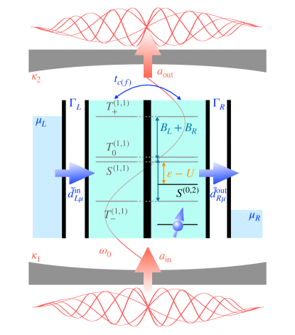
Figure 1: Schematic rendering of the DQD energy levels (without valley degree of freedom for simplicity). The DQD is coupled to source (left, $L$) and drain (right, $R$) leads as well as a resonator with two ports. The spin degeneracy is lifted by the Zeeman splitting $B_{L(R)}$. The onsite potentials $V_{j}$ of the QDs are tuned such that the right dot is always occupied by one electron. A second electron can tunnel from the source to the left QD, between the QDs via the spin conserving (flipping) tunneling $t_{c(f)}$ and from the right QD to the drain, resulting in an electric current $I$ though the system. For $\varepsilon-U=V_{L}-V_{R}-(U_{R}-U_{LR})=0$ the tunneling between the singlets is elastic. The electric dipole moment of the moving electrons couples to the electric field inside a cavity field with resonance frequency $\omega_{0}$. If the spin structure of a two-electron state is incompatible with a doubly occupied QD, Pauli blockade occurs and the current is suppressed. This is the case for the spin triplet states $T_{0(\pm)}$. The interaction with the environment is described by the input and output fields along with the coupling rates $\Gamma_{L(R)}$, $\kappa_{1(2)}$.

To model a double quantum dot where only the lowest orbital state is available we use an extended Hubbard Hamiltonian [24, 1],

$$H_{\mathrm{QD}} = \sum_{j,\sigma,v}E^{\prime}_{j\sigma v}d_{j\sigma v}^{\dagger}d_{j\sigma v}+\sum_{\sigma,\sigma^{\prime},v,v^{\prime}}\left(t_{\sigma v\sigma^{\prime}v^{\prime}}d_{R\sigma^{\prime}v^{\prime}}^{\dagger}d_{L\sigma v}\right.$$ (1)

$$\left.+\mathrm{h.c.}\right)+U_{LR}n_{L}n_{R}+\sum_{j}\frac{U_{j}}{2}n_{j}\left(n_{j}-1\right).$$

Here, $d_{j\sigma v}^{(\dagger)}$ annihilates (creates) an electron with spin $\sigma=\uparrow,\downarrow$ and valley index $v=\pm$ in QD $j=L,R$ and $n_{j}=\sum_{\sigma,v}d_{j\sigma v}^{\dagger}d_{j\sigma v}$ denotes the occupation number operator of dot $j$. We have introduced the onsite energies $E^{\prime}_{j\sigma v}=V_{j}+B_{j}(\sigma_{z})_{\sigma\sigma}/2+\Delta_{j}(\sigma_{z})_{vv}$ with the electric potential $V_{j}$, Zeeman splitting $B_{j}$ and valley splitting $\Delta_{j}$. Here, $\sigma_{z}$ denotes the Pauli $z$ matrix. Inter-dot tunneling ($t_{\sigma v\sigma^{\prime}v^{\prime}}$) can either be spin conserving, $t_{c}$, or spin flipping, $t_{f}$, and we define the valley phase difference $\varphi_{v}$ such that $t_{c(f)}\cos\varphi_{v}$ is the matrix element for intra-valley tunneling and $t_{c(f)}\sin\varphi_{v}$ is the matrix element for inter-valley tunneling. The Coulomb repulsion between electrons in adjacent QDs (the same QD) is given by $U_{LR}$ ($U_{j}$, $j=L,R$).

The resonator is modeled as a single-mode harmonic oscillator, $H_{\mathrm{res}}=\omega_{0}a^{\dagger}a$ with resonance frequency $\omega_{0}$ and ladder operator $a$. The interaction between the DQD and the resonator photons is given by [63, 64]

$$H_{\mathrm{dip}}=\frac{g_{0}}{2}\left(a^{\dagger}+a\right)\sum_{\sigma,v}\left(d_{L\sigma v}^{\dagger}d_{L\sigma v}-d_{R\sigma v}^{\dagger}d_{R\sigma v}\right).$$ (2)

We assume that each QD $j$ is coupled to one fermionic reservoir where $c_{kj\sigma v}^{(\dagger)}$ annihilates (creates) an electron with wavenumber $k$, spin $\sigma$ and valley $v$. At the same time, the resonator interacts with one photonic reservoir with ladder operator $b_{x,\omega}$ at each port $x=1,2$,

$$H_{E}=\sum_{j,k,\sigma,v}\varepsilon_{kj\sigma v}c_{kj\sigma v}^{\dagger}c_{kj\sigma v}+\sum_{x}\int\mathrm{d}\omega\,\omega b_{x,\omega}^{\dagger}b_{x,\omega}.$$ (3)

The electrons can tunnel between reservoir $j$ and QD $j$ with a matrix element $\tau_{kj\sigma v}$ and for each port of the resonator we define the coupling $g_{x}(\omega)$ to the continuum. The interaction of the electrons and the cavity photons with their respective reservoirs is described by the Hamiltonian term,

$$H_{I} = \sum_{j,k,\sigma,v}\tau_{kj\sigma v}\left(c_{kj\sigma v}^{\dagger}d_{j\sigma v}+d_{j\sigma v}^{\dagger}c_{kj\sigma v}\right)$$ (4)

$$+ \sum_{x}\int\mathrm{d}\omega\,g_{x}(\omega)\left(b_{x,\omega}^{\dagger}a+a^{\dagger}b_{x,\omega}\right).$$

To investigate Pauli blockade we restrict the system to be close to the triple point of the charge configurations $(n_{L},n_{R})=(1,1)$, $(0,2)$, $(0,1)$ where $\varepsilon=V_{L}-V_{R}$ is $\varepsilon=U$, with $U=U_{R}-U_{LR}$. Under these premises the two-electron Hilbert space of the DQD is spanned by ten supertriplet states and six supersinglets with the (1,1) charge configuration and six supersinglets with the (0,2) charge configuration [49, 65]. We separate the two-electron states into the (1,1) states $|1i\rangle$, $i=1,...16$, and the (0,2) states $|2i\rangle$, $i=1,...6$. If the valley degree of freedom is disregarded, the (1,1) states form a spin triplet and one singlet and there is one (0,2) singlet. We further introduce the operators $d_{\mu}$ that remove one electron from eigenstate $\mu=1,...22$ with energy $E_{\mu}$ of $H_{\mathrm{QD}}$ with two electrons.

II.2 Input-Output Theory

Input-output (IO) theory is a powerful tool for the modelling of cavity-coupled qubits [66, 58, 6]. Here, we apply a generalized version to combine the treatment of the electronic transport process and the description of the resonator field in one formalism [62].

First, the Hamiltonian is transformed into a rotating frame, $\tilde{H}=U_{r}HU_{r}^{\dagger}+i(\frac{\mathrm{d}}{\mathrm{d}t}U_{r})U_{r}^{\dagger}$, denoted by the tilde and defined by

$$U_{r}=\exp(-i\omega_{p}a^{\dagger}a)\exp\left(-i\sum_{\mu}\Omega_{\mu}\tilde{d}_{\mu}^{\dagger}\tilde{d}_{\mu}\right),$$ (5)

with the frequency $\omega_{p}$ of the probe field that is injected into the resonator. The transformation on the electronic states is not unique and can be chosen by setting $\Omega_{\mu}$. For example, to observe transitions between levels adjacent in energy one can define $E_{\mu}\leq E_{\mu+1}$ and $\Omega_{\mu}=\omega_{p}(\mu-1)$.

Following the procedures of IO theory [66, 62], the Heisenberg equations of motion for the reservoir operators are formally integrated to eliminate the reservoir operators in the equations of motion of the system operators. This results in the Langevin equations,

$$\frac{\mathrm{d}}{\mathrm{d}t}\tilde{a} = -(i\Delta_{c}+\kappa/2)\tilde{a}+\sum_{x=1,2}\sqrt{\kappa_{x}}\tilde{a}_{\mathrm{in},x}$$ (6)

$$-i\sum_{\mu,\nu}g_{\mu\nu}e^{-i(\omega_{p}-\Omega_{\nu}+\Omega_{\mu})(t-t_{0})}\tilde{d}_{\nu}^{\dagger}\tilde{d}_{\mu},$$

$$\frac{\mathrm{d}}{\mathrm{d}t}\tilde{d}_{\mu} = -\left[i(E_{\mu}-\Omega_{\mu})+\sum_{j=L,R}\left(1-n_{F}^{j}(E_{\mu})\right)\tilde{\Gamma}_{j\mu}\right]\tilde{d}_{\mu}$$ (7)

$$-i\sum_{\nu}\left(g_{\nu\mu}ae^{i(\omega_{p}-\Omega_{\mu}+\Omega_{\nu})(t-t_{0})}+\mathrm{h.c.}\right)\tilde{d}_{\nu}$$

$$+\sqrt{2\pi}\left(\tilde{d}_{L\mu}^{\mathrm{in}}(t)+\tilde{d}_{R\mu}^{\mathrm{in}}(t)\right)\left(1-\sum_{\nu}\tilde{d}_{\nu}^{\dagger}\tilde{d}_{\nu}\right).$$

Here, we defined $\Delta_{c}=\omega_{0}-\omega_{p}$, the coupling matrix elements $g_{\nu\mu}=g_{0}\sum_{i}\langle\nu|2i\rangle\langle 2i|\mu\rangle$ and introduced the Fermi distribution function $n_{F}^{j}$ such that lead $j=L,R$ is described by its Fermi energy $\mu_{j}$ and the temperature $T$. The coupling to the environment is captured in the rates

$$\kappa = \sum_{x}\kappa_{x}\approx 2\pi\sum_{x}g_{x}^{2}(\omega),$$ (8)

$$\tilde{\Gamma}_{L\mu} = \pi\sum_{k,\sigma,v}\left|\sum_{i}\langle 1i|\mu\rangle\tau_{Lk\sigma v}\right|^{2}\delta(\varepsilon-\varepsilon_{kL\sigma v}),$$ (9)

$$\tilde{\Gamma}_{R\mu} = \pi\sum_{k,\sigma,v}\left|\sum_{i}\langle 2i|\mu\rangle\tau_{Rk\sigma v}\right|^{2}\delta(\varepsilon-\varepsilon_{kR\sigma v})$$ (10)

and the input fields

$$\tilde{a}_{\mathrm{in,x}} = \frac{-i}{\sqrt{2\pi}}\int\mathrm{d}\omega e^{-i\omega(t-t_{0})}b_{x,\omega}(t_{0})$$ (11)

$$\tilde{d}_{j\mu}^{\mathrm{in}}(t) \approx \frac{-i}{\pi}\sqrt{\frac{\tilde{\Gamma}_{j\mu}}{2}n_{F}^{j}(E_{\mu})}\,e^{-i(E_{\mu}-\Omega_{\mu})(t-t_{0})}.$$ (12)

The derivation of these expression relies on the approximations that the couplings between the resonator and the environment is flat, $g_{x}(\omega)\approx g_{x}$, and that the electronic reservoir of the leads are infinite. As a reference we also define the total tunneling rates between dot $j=L,R$ and its lead,

$$\Gamma_{j}\approx\pi\sum_{k}|\tau_{kj\sigma v}|^{2}\delta(\varepsilon-\varepsilon_{jk\sigma v}),$$ (13)

assuming that $\tau_{kj\sigma v}\approx\tau_{kj}$. For simplicity we will further choose $\Delta_{c}=0$ and $t-t_{0}\gg 1/\kappa,1/\tilde{\Gamma}_{L(R)}$ throughout the remainder of the paper.

We assume that the resonator is driven with a coherent input field from one port only, $\tilde{a}_{\mathrm{in},1}=a_{\mathrm{in}}$, $\tilde{a}_{\mathrm{in},2}=0$. Unlike Ref. [62] we proceed by formally integrating the equation for the field $\tilde{a}$ to

$$\tilde{a}(t) = \int_{t_{0}}^{t}\mathrm{d}t^{\prime}\,e^{-\kappa(t-t^{\prime})/2}\Bigg{(}\sqrt{\kappa_{1}}a_{\mathrm{in}}$$ (14)

$$-i\sum_{\mu,\nu}g_{\mu\nu}e^{-i(\omega_{p}+\Omega_{\mu}-\Omega_{\nu})t^{\prime}}\tilde{d}_{\mu}^{\dagger}(t)\tilde{d}_{\nu}(t)\Bigg{)}$$

and we apply a rotating wave approximation (RWA) which is justified for $|\omega_{0}-(E_{\mu}-E_{\nu})|\ll E_{\mu}-E_{\nu}\approx\omega_{p}$ [67]. Introducing the auxiliary variable $N_{\mu\nu}=\tilde{d}_{\mu}^{\dagger}\tilde{d}_{\nu}$ the remaining system of equations is Laplace transformed.

The time dependent exponential functions result in a shift in the complex frequency space [68] which can be expressed by defining a displacement operator $\mathcal{S}_{x}f(s)=f(s+x)$ with $\mathcal{S}_{x}^{-1}=S_{-x}$. The resulting system of linear equations can be solved for $\mathcal{L}\tilde{d}_{\mu}(s)$, the Laplace-transform of $\tilde{d}_{\mu}(t)$ [69]:

$$\mathcal{L}\tilde{d}_{\mu}(s) = \sum_{\nu}(A_{0}^{-1})_{\mu\nu}(s)C_{\nu}(s)+\sum_{\nu,\lambda,\eta}(A_{0}^{-1})_{\mu\nu}(s)(A_{1})_{\nu\lambda}(s)(A_{0}^{-1})_{\lambda\eta}\left[s+i(E_{\lambda}-E_{\eta}-\Omega_{\lambda}+\Omega_{\eta})\right]C_{\eta}(s)$$ (15)

$$-\sum_{\nu,\lambda,\eta}(A_{0}^{-1})_{\mu\nu}(s)(A_{1})_{\nu\lambda}(s)(A_{0}^{-1})_{\lambda\eta}^{*}\left[s+i(E_{\lambda}+E_{\eta}-\Omega_{\lambda}-\Omega_{\eta})\right]C_{\eta}^{*}(s),$$

where the initial conditions at $t_{0}$ enter via

$$C_{\mu}(s)=\sqrt{2\pi}\hat{d}_{\mu}^{\mathrm{in}}\left[\frac{1}{s+i(E_{\mu}-\Omega_{\mu})}-\sum_{\nu}\frac{\tilde{N}_{\nu\nu}(t_{0})}{s+2\gamma_{\nu}}\right]+\tilde{d}_{\mu}(t_{0}).$$ (16)

and the coefficient matrices are

$$(A_{0})_{\mu\nu}(s) = \delta_{\mu\nu}\left\{s+\left[i\left(E_{\mu}-\Omega_{\mu}\right)+\gamma_{\mu}\right]\right\}+ip_{\mu\nu},$$ (17)

$$(A_{1})_{\mu\nu}(s) = 2\pi\hat{d}_{\mu}^{\mathrm{in}}\left(\hat{d}_{\nu}^{\mathrm{in}}\right)^{*}(s+2\gamma_{v})^{-1},$$ (18)

$$\hat{d}_{\mu}^{\mathrm{in}} = \frac{-i}{\pi}\sum_{j=L,R}\sqrt{\frac{\tilde{\Gamma}_{j\mu}}{2}\,n_{F}^{j}(E_{\mu})},$$ (19)

$$\gamma_{\mu} = \sum_{j=L,R}\left(1-n_{F}^{j}(E_{\mu})\right)\tilde{\Gamma}_{j\mu},$$ (20)

$$p_{\mu\nu} = 4\frac{g_{0}}{\kappa}|a_{\mathrm{in}}|\delta\left(\omega_{p}-\Omega_{\nu}+\Omega_{\mu}\right)+q_{\mu\nu}.,$$ (21)

where $\delta_{\mu\nu}$ is the Kronecker symbol and $\delta$ is the $\delta$-distribution. The term $q_{\mu\nu}$ in Eq. (21) can be understood as a back-action of the DQD on itself via the resonator. It can be expected to be small and is neglected in the discussion in Secs. III and IV. An estimate for the case $\kappa\ll\Gamma_{L},\Gamma_{R}$ is given by

$$q_{\mu\nu} \lesssim \sqrt{2\pi}\,g_{0}^{2}\zeta_{\mu\nu}2e^{-\kappa\tau/2}\left|\sum_{\lambda}\hat{d}_{\lambda}^{\mathrm{in}}\right|^{2},$$ (22)

$$\zeta_{\mu\nu} = \mathrm{sgn}\left\{(\Omega_{\nu}-\Omega_{\mu})\cos\left[(\Omega_{\nu}-\Omega_{\mu})\tau\right]\right\},$$ (23)

$$\tau = 2\mathrm{max}_{\lambda,\eta}|\Omega_{\lambda}-\Omega_{\eta}|/(\kappa\Gamma_{R}),$$ (24)

where $\mathrm{sgn}$ is the sign function.

Although the Laplace transform $\mathcal{L}\tilde{d}_{\mu}$ itself has no physical meaning, the steady state solution of the Langevin equations can be obtained from Eq. (15) by the identity

$$\lim_{t\to\infty}\tilde{d}_{\mu}(t)=\lim_{s\to 0+}s\mathcal{L}\tilde{d}_{\mu}(s)$$ (25)

if $\mathcal{L}\tilde{d}_{\mu}$ has no other singularities with $\mathrm{Re}\,s\geq 0$ than a pole at $s=0$ [68]. Alternatively, an inverse Laplace transform of Eq. (15) yields the real-time dynamics of $\tilde{d}_{\mu}(t)$ for $t-t_{0}\gg 1/\kappa,1/\tilde{\Gamma}_{L(R)}$. Substituting into Eq. (14) gives the time evolution of $\tilde{a}$, the output field $a_{\mathrm{out}}$ is obtained from the IO relations [66]. Eventually, the current from the DQD to the drain contact in units of electron charges $e$ is given by $I/e=\frac{\mathrm{d}}{\mathrm{d}t}\sum_{k,\sigma,v}\left\langle c_{kR\sigma v}^{\dagger}c_{kR\sigma v}\right\rangle$, which can be expressed using the IO relation [62],

$$I=2e\sum_{i,\mu}|\langle 2i|\mu\rangle|^{2}\left(\Gamma_{R}\left\langle\tilde{d}_{\mu}^{\dagger}\tilde{d}_{\mu}\right\rangle-\sqrt{2\pi}\mathrm{Re}\left\langle\tilde{d}_{\mu}^{\dagger}\tilde{d}_{R\mu}^{\mathrm{in}}\right\rangle\right).$$ (26)

The first term in Eq. (26) describes the decay of population in the right QD to the right lead with a decay rate $\Gamma_{R}$ computed from IO theory. The second term describes tunneling from the right lead to the DQD which becomes relevant with high temperatures or a small bias window $\mu_{L}-\mu_{R}$. We emphasize that the solution using Eq. (25) is analytic, although it requires the (numerical) diagonalization of $H_{\mathrm{QD}}$.

It is also possible to solve the Laplace-transformed equations without RWA. The analogue of Eq. (15) beyond the RWA is presented in Appendix A. We further note that it is straightforward to generalize our theory to a QD system with arbitrary geometry coupled to any number of resonators.

III Discussion

We first investigate the basic properties of the interaction without valley degree of freedom. In this case the (1,1) triplets ($T_{0(,\pm}$) are blockaded unless spin-flip processes allow transitions to the (0,2) singlet ($S^{(0,2)}$). The solution with RWA is used and the stationary state is obtained from Eq. (25). We assume a bias window of $\mu_{L}-\mu_{R}=$1\text{\,}\mathrm{meV}$$, centered around the DQD levels and $T=$0.1\text{\,}\mathrm{K}$$.

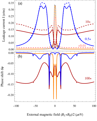
Figure 2: Comparison of the leakge current and the cavity response in different regimes. (a) Leakage current $I$ as a function of the Zeeman splitting. The orange curve has small tunneling $t_{c}^{2}+t_{f}^{2}=$1\text{\,}\mathrm{\SIUnitSymbolMicro eV}$^{2}$, $B_{R}-B_{L}=$14\text{\,}\mathrm{\SIUnitSymbolMicro eV}$$ and $\omega_{0}=\sqrt{2}\,$5\text{\,}\mathrm{\SIUnitSymbolMicro eV}$$. The red (blue) curve have strong tunneling $t_{c}=$20\text{\,}\mathrm{\SIUnitSymbolMicro eV}$$ and the magnetic field gradient $B_{R}-B_{L}=$1.5(10)\text{\,}\mathrm{\SIUnitSymbolMicro eV}$$ and $\omega_{0}=\sqrt{2}\,$20\text{\,}\mathrm{\SIUnitSymbolMicro eV}$$. For all curves we chose $t_{c}=4t_{f}$, $\varepsilon=U$, $g_{0}=$0.5\text{\,}\mathrm{\SIUnitSymbolMicro eV}$$, $\kappa=$1.28\text{\,}\mathrm{\SIUnitSymbolMicro eV}$$, $\Gamma_{L}=2\Gamma_{R}=$10\text{\,}\mathrm{\SIUnitSymbolMicro eV}$$, $a_{\mathrm{in}}=$1\text{\,}\mathrm{\SIUnitSymbolMicro}\mathrm{eV}^{1/2}$$. The dashed curves have the same setting as their solid counterparts (light red corresponds to orange) except $\kappa=$0.0128\text{\,}\mathrm{\SIUnitSymbolMicro eV}$$ to highlight the back-action of the photons on the DQD. The dashed gray curve has the same setting as the orange curve but is obtained from a numerical treatment of the system, the agreement with the analytically approximated solution is very good. For clarity the red (blue) curves are scaled up (down) by a factor of 10 (0.5) and the light red curve is offset by $0.01e/$\mathrm{ns}$$. Note that $\Gamma_{R}$ is relatively small, here. (b) Phase shift $\delta\varphi$ of outgoing photons in the same cases. Up to narrow resonances $E_{\mu}-E_{\nu}=\omega_{p}$ the phase shift correlates with the current $I$; the connection is established by Eqs. (14) and (26).

In Fig. 2(a) the leakage current $I$ is plotted for different values of the total tunneling and the difference in Zeeman splitting, $B_{L}-B_{R}$. The dashed gray curve is based on an exact numerical treatment of the system for the same parameters as the orange curve. The agreement with the approximate analytical solution is very good. Note, however, that some curves are missing a narrow window around $B_{L}+B_{R}=0$. In these cases the limit of Eq. (25) is undefined. An inverse Laplace transform of Eq. (15) can still yield the solution at these instances, at a much higher computational cost.

As the figure shows, the model can reproduce the features known to appear in spin blockade. The leakage current exhibits a transition from a Lorentzian dip to a peak at zero magnetic field when the tunneling is decreased [31]. For large magnetic fields the current decays to zero [36, 37] to the extent that it can appear as a double peak with the width determined by $\Gamma_{R}$ [70]. We also observe a small dip at $B_{L}+B_{R}=\pm 2\sqrt{2}t_{c}$ where the strongly hybridized singlets anticross with the $T_{\pm}$ triplet states that are only weakly coupled to the $(0,2)$ sector since the degenerate levels rearrange into blockaded and open states [31].

The phase shift $\delta\varphi=\arg\;a_{\mathrm{out}}/a_{\mathrm{in}}$, displayed in Fig. 2(b), responds to the current since the photons couple to the dipole moment of the tunneling electrons, as can be expected from Eqs. (14) and (26). Thus, it is possible to qualitatively infer the relative change of the leakage current from $\delta\varphi$ during the sweep. However, to estimate the value of $I$ it is import to respect the dependence of $g_{\mu\nu}$ of the levels $\mu,\nu$ that carry current on the DQD parameters, and to consider how close $\omega_{p}$ is to a resonance with the DQD level splitting. In the example this is highlighted by comparing the cases of strong (blue) and weak (orange) tunneling both with strong magnetic gradient. Even though the maximal current in the blue curve is twice as high as the maximum of the orange curve, the resonator response is weaker due to different effective couplings.

The resonator response $\delta\varphi$ also exhibits narrow peaks where the probe field is resonant with a DQD level transition, $\omega_{p}=E_{\mu}-E_{\nu}$. These resonances could disturb a resonator-aided measurement of the leakage current if the level structure of the DQD is unknown.

Furthermore, there can be a significant back-action of the resonator photons on the current $I$. The dashed curves in Fig. 2(a) strongly deviate from their solid counterparts, although the only difference is a smaller value of $\kappa$. The reason is that absorption or emission of photons can lead to a different electronic equilibrium state than without the resonator. In particular, near the avoided level crossings (ALCs) between singlet and triplet states the electron can be excited from a triplet to a singlet which has much higher probability for a transition to the drain. Vice versa, excitation from a singlet to a triplet reduces the current.

To estimate the magnitude of this effect we treat the ALCs between the singlets and the $T_{0}$ ($T_{\pm}$) at $B_{L}+B_{R}=\pm 0$ ($B_{L}+B_{R}=2\sqrt{2}t_{c}$) separately with an effective three (two) level Hamiltonian. In both cases we find that the current has the form

$$I^{\prime}\approx I_{0}+p_{0}\sqrt{I_{0}}\delta$$ (27)

with $p_{0}=4g_{0}|a_{\mathrm{in}}|/\kappa$, the current $I_{0}$ through the uncoupled DQD and a correction $\delta$. Thus, in strongly driven high-Q resonators it can be expected that the current is altered by the resonator. The explicit expressions that describe the relative change of $I$ near these ALCs are given in Appendix B.

We further find that in the off-resonant dispersive regime $g_{\mu\nu}\ll|\omega_{p}-(E_{\mu}-E_{\nu})|$ [67] the leakage current $I(\varepsilon)$ appears to be displaced along the detuning axis $\varepsilon$ if $p_{0}$ is large. This can be understood by the well-known dispersive shift of the energy splittings to which the DQD-photon interaction is reduced in the dispersive regime. The shift $\chi_{m}(a^{\dagger}a+1/2)$ of the molecular transition frequencies [20] affects only the (0,2) singlet state and appears as a shift of $\varepsilon\to\varepsilon-2\chi_{m}(a^{\dagger}a+1/2)$ near the ALC of the singlets at $\varepsilon=0$.

IV Lifted Valley Degeneracy

In this section the repercussions of the valley degree of freedom are discussed. This case is important for conduction-band electron transport through silicon DQDs with near-degenerate valleys. Eventually, we present schemes to estimate the leakage current in Sec. IV.1 and to measure the parameters of the (valley) Hamiltonian from the resonator response during a transport experiment in Sec. IV.2.

Now, there are 16 (1,1) states with subtle conditions to be blockaded [48, 49, 50, 39]. The effects discussed in Sec. III – a resonator response to the leakage current and back-action of both resonant and off-resonant photons in the current for large $p_{0}$ – are present in this case as well. However, in the more complex level diagram there are many transitions between different supersinglet and -triplet states that can interact with the resonator.

We use the analytic result Eq. (25) to identify each eigenstate’s contribution to leakage current and transmission. Approximating the DQD levels, we find that for $t_{c}\gg t_{f}$ any of the following resonance conditions can give rise to a strong resonator response.

$$\omega_{p} \approx \sqrt{2}|t_{c}\cos\varphi_{v}|,$$ (28)

$$\omega_{p}^{2} \approx \left[(\varepsilon-U)\pm\frac{B_{L}-B_{R}}{2}\pm\frac{\Delta_{L}+\Delta_{R}}{2}\right]^{2}$$ (29)

$$+4(t_{c}\sin\varphi_{v})^{2},$$

$$\omega_{p}^{2} \approx \left[(\varepsilon-U)\pm\frac{B_{L}+B_{R}}{2}\pm\frac{\Delta_{L}+\xi\Delta_{R}}{2}\right]^{2}$$ (30)

$$+4(t_{f}\lambda_{\xi})^{2}$$

with $\xi=\pm 1$, $\lambda_{-1}=\cos\varphi_{v}$, $\lambda_{1}=\frac{1}{\sqrt{2}}\sin\varphi_{v}$ and also

$$\omega_{p}^{2}\approx\left[(\varepsilon-U)-\xi\Delta_{R}\pm\frac{B_{L}-B_{R}}{2}\right]^{2}+4(t_{f}\lambda_{\xi})^{2}$$ (31)

with $\xi=0,\pm 1$, $\lambda_{\pm 1}=\frac{1}{\sqrt{2}}\sin\varphi_{v}$, $\lambda_{0}=\cos\varphi_{v}$. Note that Eq. (28) is a good approximation only for $\varepsilon=U$. A more accurate expression is given in Appendix C.

Due to the different couplings $g_{\mu\nu}$ the resonances Eq. (28-31) have different visibilities in the resonator response. This can be seen in Fig. 3(a) where $I$ is plotted together with $\delta\varphi$ for two different values of $\omega_{p}$.

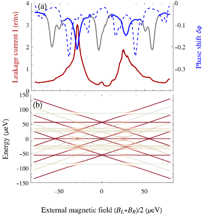
Figure 3: The phase shift $\delta\varphi$ can be used to estimate the leakge current except in the vicinity of particular ALCs. (a) Current $I$ (red) and phase shift $\delta\varphi$ (blue, gray) with valley. The solid (dashed) curve of $\delta\varphi$ is computed with $\omega_{p}=$60\text{\,}\mu\mathrm{eV}$$ ($\omega_{p}=$40\text{\,}\mu\mathrm{eV}$$) and thus the resonances Eq. (28-31) are met at different values of $B_{L}+B_{R}$. The choice for the solid curve is according to the scheme to measure $I$ discussed in Sec. IV.1, the intervals with gray curve are those where the measurement cannot yield clear information on $I$. (b) Level diagram of the DQD. The darker red a curve is the less overlap has the corresponding state with the (0,2) sector, dark red states are blockaded. Parameters for both panels are $\Delta_{L}=$50\text{\,}\mathrm{\SIUnitSymbolMicro eV}$$, $\Delta_{R}=$60\text{\,}\mathrm{\SIUnitSymbolMicro eV}$$, $\varphi_{v}=\pi/13$, $t_{c}=4t_{f}=$20\text{\,}\mathrm{\SIUnitSymbolMicro eV}$$, $B_{L}-B_{R}=2\kappa=$10\text{\,}\mathrm{\SIUnitSymbolMicro eV}$$. The rest is as in Fig. 2.

IV.1 Observation of the Leakage Current

During a sweep of $\varepsilon$, the Zeeman splitting or the tunneling multiple of the resonances Eqs. (28)-(31) can be traversed. As a result, similar values of $I$ can appear with different visibility in $\delta\varphi$ since the relevant resonances are associated with different dipole moments. In the example of Fig. 3(a), the dashed curve is not suited to extract information on $I$ since the resonances are met on the flanks of the peaks of $I$.

This challenge can be partially mitigated, if the measurement is performed with $\varepsilon\approx 0$, $\kappa\gtrsim|B_{L}-B_{R}|/2$ and $\omega_{p}\approx(\Delta_{L}+\Delta_{R})/2+t_{f}$. With this choice of $\omega_{p}$ the probe field is approximately resonant with the splitting between (1,1) supertriplets with equal spin and opposite valley configuration (red in Fig. 3(b)). The resonator field is therefore sensitive to ALCs involving these states which lift the blockade. The choice of $\kappa$ is necessary since the supertriplet states without spin polarization are shifted by the difference in Zeeman splitting. An advantage of a relatively large $\kappa$ is the suppression of unwanted back-action effects.

The result during a sweep of $B_{L}+B_{R}$ is depicted in Fig. 3(a) by the solid curve. The figure also highlights the limitation of this method. Near ALCs of supertriplets with opposite spin at

$$B_{L}+B_{R} = 0,$$ (32)

$$B_{L}+B_{R} = \frac{B_{L}-B_{R}}{2},$$ (33)

$$B_{L}+B_{R} = \pm(\Delta_{L}+\Delta_{R}+2t_{f}),$$ (34)

the correlation of resonator response and leakage current is broken and the phase shift is much stronger as can be expected from $I$. In a window of $\approx 4\kappa$ around these ALCs the resonator-aided measurement of the leakage current is not reliable. These intervals are indicated in Fig. 3(a) by changing the color of the curve to gray.

Thus, the utility of the proposed measurement scheme to observe the leakage current is limited by the mean valley splitting $(\Delta_{L}+\Delta_{R})/2$ and the difference in Zeeman splitting $|B_{L}-B_{R}|$ to which $\kappa$ is tied. Another practical limitation to certain regimes might arise from the requirement to set $\omega_{p}$ to a value determined by the valley splitting. In silicon-based heterostructures the valley splitting is sensitive to the fabrication details [51, 52, 53] and electrically tunable only in a limited range [53, 55, 56, 57], in bilayer graphene the valley splitting can be tuned by means of an out-of-plane magnetic field [71] which also couples to the spin magnetic moment.

IV.2 DQD Characterization

It is favourable to know the valley splittings $\Delta_{L(R)}$ and the valley phase $\varphi_{s}$ for a given DQD device. In the context of Pauli blockade this is important since the ratio of the different tunneling matrix elements has a major effect on $I$, as a comparison of the leakage current in Figs. 3 and 4 shows. Furthermore, when using the scheme discussed in Sec. IV.1 to measure the leakage current knowledge about the valley splitting is crucial to set $\omega_{p}$ and to determine the windows of unreliable results that should be clipped.

This knowledge can be inferred from a prior measurement using well-established protocols and the same microwave resonator [58, 59, 60, 61]. Here, we present an alternative resonator-aided scheme for the DQD characterization during a transport experiment.

For this application the resonance condition Eq. (28) can be used, $\omega_{p}\approx\sqrt{2}|t_{c}\cos\varphi_{v}|$, with $\varepsilon=U$. Thus, the probe field is resonant with the splitting between the energy levels $\hat{E}_{1(3)}$ and $\hat{E}_{2}$ approximately given by Eq. (55-56) in Appendix D. The ALCs of these states with $\hat{E}_{1}^{\prime}-\hat{E}_{6}^{\prime}$, Eq. (57-61), during a sweep of the magnetic field give rise to an extremum in the resonator response, each. This is depicted in Fig. 4. Unknown DQD parameters can then be inferred by equating the expressions from Appendix D and solving for the unknown DQD parameters.

The performance of this scheme is limited by two possible caveats. First, the ALCs might be closer than the resonator linewidth $\kappa/2$ and can thus not be resolved individually. This is shown in Fig. 4 near $(B_{L}+B_{R})/2=$37\text{\,}\mathrm{\SIUnitSymbolMicro eV}$$. Second, some of the other resonance conditions, Eq. (28-31), might be met during the sweep, giving rise to an unexpected extremum. This is shown by the cyan highlight in Fig. 4. In both cases it is not impossible to infer unknown DQD parameters but since it is unclear which extrema belong to which equation additional effort is necessary to find a consistent mapping.

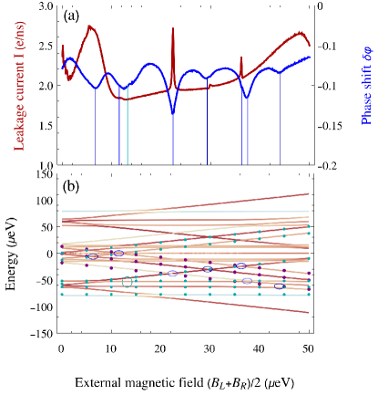
Figure 4: Outline of the measurement of unknown DQD parameters. (a) The phase shift $\delta\varphi$ is measured with $\omega_{p}=\sqrt{2}|t_{c}\cos\varphi_{v}|$. Note that here $\omega_{p}$ is not at the ideal point for measuring $I$ (Sec. IV.1), thus $\delta\varphi$ cannot be used to reliably quantify $I$. (b) In the level diagram, the extrema of $\delta\varphi$ can be related to the ALCs between $\tilde{E}_{1}-\tilde{E}_{3}$ (purple dotted) and $\tilde{E}_{1}^{\prime}-\tilde{E}_{6}^{\prime}$ (cyan dotted), as indicated by the blue vertical lines and matching ellipses. Additional resonances (cyan ellipse) or very close ALCs can obscure the result. Parameters for both panels are the same as Fig. 3 up to $\omega_{p}=\sqrt{2}\,$10\text{\,}\mathrm{\SIUnitSymbolMicro eV}$$ and $\varphi_{s}=\pi/3$. The darker red a curve in (b) is the less overlap has the corresponding state with the (0,2) sector. Due to the strong valley-flip tunneling no state is totally blockaded.

V Summary and Conclusion

In this article we extended the generalized IO theory and derived an analytic description of electronic transport in the Pauli blockade regime in semiconductor quantum dots coupled to a microwave resonator. We first investigated the interaction of a spin blockade with the microwave photons within a RWA, although we also provide a solution beyond the RWA. While the resonator’s output field carries quantitative information on the leakage current, there can also be back action on the current. Near the resonance of the probe field with a DQD transition, this is due to the absorption of photons. Away from resonance the mutual dispersive shift of DQD and resonator may also obscure experimental results. We analytically estimated the change of the leakage current and concluded that back-action can be mitigated by choosing parameters where $p_{0}=4g_{0}|a_{\mathrm{in}}|/\kappa$ is small.

In the case of a lifted valley degeneracy, i.e. for silicon or carbon based spin qubits, the back-action effects persist. The resonator response to the leakage current, however, can show a complicated dependence due to different resonance conditions with a large number of states. As a result, there is not necessarily a quantitative agreement between $\delta\varphi$ and $I$. Nonetheless, we devised a scheme that allows to observe the leakage current from a measurement of the output field, limited by the valley splitting and the difference in Zeeman splitting between the QDs. Furthermore, we provide a scheme that can be used to extract information on unknown DQD parameters simultaneous to a transport experiment.

Pauli blockade is a powerful tool for the characterization of spin qubits. Our results can help leveraging its utility to large-scale qubit applications without dedicated components for charge or current sensing in each QD. This can be useful because the same resonator used for two-qubit gates and possibly readout can accomplish this task. The back-action described here can open a novel pathway to manipulate the electronic state of a QD system by enhancing or suppressing a leakage current. For future research directions, applications relevant for photonic platforms are also worth investigating. For example, a tunable interaction between two resonators coupled to the same DQD is conceivable, harnessing the properties of Pauli blockade and the back-action.

Appendix A Solution beyond the RWA

The solution of the Langevin equations derived in the main text and used for the discussion of the interaction was based on a rotating wave approximation (RWA). The RWA is not strictly necessary to solve the problem. Here, we give the analogue of Eq. (15) without RWA:

$$\mathcal{L}\tilde{d}_{\mu}(s) = \sum_{\nu}(\hat{A}_{0}^{-1})_{\mu\nu}(s)C_{\nu}(s)-\frac{2i}{p_{0}}\sum_{\nu}\left\{C_{\nu}[s-i(\omega_{p}-\Omega_{\nu}-\Omega_{\mu})]+C_{\nu}[s+i(\omega_{p}-\Omega_{\nu}-\Omega_{\mu})]\right\}$$

$$+\sum_{\lambda}\Big{\{}\sum_{\nu}(\hat{A}_{0}^{-1})_{\mu\lambda}(s)(A_{1})_{\nu\lambda}(s)-\frac{2i}{p_{0}}\sum_{\nu}\left\{(A_{1})_{\nu\lambda}[s-i(\omega_{p}-\Omega_{\nu}-\Omega_{\mu})]+(A_{1})_{\nu\lambda}[s+i(\omega_{p}-\Omega_{\nu}-\Omega_{\mu})]\right\}\Big{\}}$$

$$\sum_{\eta}\Bigg{\{}(\hat{A}_{0}^{-1})_{\lambda\eta}[s+i(E_{\lambda}-E_{\eta}-\Omega_{\lambda}+\Omega_{\eta})]C_{\eta}(s)-(\hat{A}_{0}^{-1})_{\lambda\eta}^{*}[s+i(E_{\lambda}+E_{\eta}-\Omega_{\lambda}-\Omega_{\eta})]C_{\eta}(s)^{\dagger}$$

$$-\frac{2i}{p_{0}}\sum_{\zeta}\big{\{}C_{\zeta}[s+i(E_{\lambda}-E_{\eta}-\Omega_{\lambda}+\Omega_{\zeta}-\omega_{p})]+C_{\zeta}[s+i(E_{\lambda}+E_{\eta}-\Omega_{\lambda}+2\Omega_{\eta}-\Omega_{\zeta}+\omega_{p})]$$

$$+C_{\zeta}^{\dagger}[s+i(E_{\lambda}+E_{\eta}-\Omega_{\lambda}-2\Omega_{\eta}+\Omega_{\zeta}-\omega_{p})]+C_{\zeta}\dagger[s+i(E_{\lambda}+E_{\eta}-\Omega_{\lambda}-\Omega_{\zeta}+\omega_{p})]\big{\}}\Bigg{\}},$$

with the new definitions

$$(\hat{A}_{0})_{\mu\nu} = \delta_{\mu\nu}\left\{s+\left[i\left(E_{\mu}-\Omega_{\mu}\right)+\gamma_{\mu}\right]\right\},$$ (36)

$$p_{0} = 4g_{0}|a_{\mathrm{in}}|/\kappa.$$ (37)

Appendix B Estimation of the back-action

To assess the magnitude of the back-action if $\omega_{p}$ is resonant to a singlet ($S$)-triplet ($T$) ALC we use reduced Hamiltonians of the states contributing to these ALCs. In both cases Eq. (25) yields the current

$$I^{\prime} \approx \frac{2\Gamma_{R}}{\hbar}\frac{|k_{c}|^{2}}{N^{2}},$$ (38)

$$k_{c} = \left(\beta+\frac{p_{0}}{\alpha}\beta^{\prime}\right)\prod_{\mu}N_{\mu}^{-1}$$ (39)

with the following definition:

$$\alpha = \sum_{\mu}|\hat{d}_{\mu}^{\mathrm{in}}|^{2}\prod_{\nu\neq\mu}\gamma_{\nu}(E_{1}-i\gamma_{\nu})$$ (40)

$$+\prod_{\mu}\frac{\gamma_{\mu}}{\pi}(E_{1}-i\gamma_{\mu})$$

$$\beta = \sum_{\mu}\hat{d}_{\mu}^{\mathrm{in}}\prod_{\nu\neq\mu}N_{\nu}(E_{1}-i\gamma_{\nu})$$ (41)

$$N^{2} = \sum_{\mu}\pi|\hat{d}_{\mu}^{\mathrm{in}}|^{2}\prod_{\nu\neq\mu}\gamma_{\nu}(E_{1}^{2}+\gamma_{\nu}^{2}).$$ (42)

Near $B_{L}+B_{R}=0$ with the three-level system

$$H_{T_{0}}=\begin{pmatrix}0&\frac{B_{L}-B_{R}}{2}&0\\ \frac{B_{L}-B_{R}}{2}&0&\sqrt{2}t_{c}^{*}\\ 0&\sqrt{2}t_{c}&U-\varepsilon\end{pmatrix}$$ (43)

in the basis $\{|T_{0}^{(1,1)}\rangle,|S^{(1,1)}\rangle,|S^{(0,2)}\rangle\}$ it is furthermore

$$\beta^{\prime} = \alpha\left[N_{1}\hat{d}_{1}^{\mathrm{in}}\sum_{\mu=1,2}N_{\nu}(E_{1}-i\gamma_{\nu})+N_{2}N_{3}\delta\right]$$ (44)

$$+\beta\Big{[}\gamma_{2}\gamma_{3}(\hat{d}_{1}^{\mathrm{in}})^{*}\delta-i\gamma_{1}\hat{d}_{1}^{\mathrm{in}}(\gamma_{3}(\hat{d}_{2}^{\mathrm{in}})^{*}(iE_{1}\gamma_{3})$$

$$+\gamma_{2}(\hat{d}_{3}^{\mathrm{in}})^{*}(iE_{1}\gamma_{2}))\Big{]}$$

$$\delta = \hat{d}_{2}^{\mathrm{in}}(E_{1}-i\gamma_{3})+\hat{d}_{3}^{\mathrm{in}}(E_{1}-i\gamma_{2})$$ (45)

$$N_{\mu} = \Bigg{[}4\Bigg{|}\frac{t_{c}}{B_{L}-B_{R}+E_{1}}\Bigg{|}^{2}+\Bigg{|}\frac{E_{1}+(\mu-1)\omega_{p}+2(\varepsilon-U)}{2t_{c}}$$ (46)

$$-\frac{2t_{c}^{*}}{B_{L}-B_{R}+E_{1}+(\mu-1)\omega_{p}}\Bigg{|}^{2}+1\Bigg{]}^{1/2}.$$

Expanding this result to first order in $p_{0}$ results in the form of Eq. (27).

Analogously, near the ALCs of the $T_{\pm}$ triplets with each singlet branch approximated by the two-level system

$$H_{T_{\pm}}=\begin{pmatrix}\pm\frac{B_{L}+B_{R}}{2}&t_{f}^{*}\\ t_{f}&U-\varepsilon\end{pmatrix}$$ (48)

in the basis $\{|T_{\pm}^{(1,1)}\rangle,|S^{(0,2)}\rangle\}$ it is

$$\beta^{\prime} = \left(\alpha-\prod_{\mu}\frac{\gamma_{\mu}}{\pi}(E_{1}-i\gamma_{\mu})\right)\left(\gamma_{1}N_{2}(\hat{d}_{2}^{\mathrm{in}})^{*}-\gamma_{2}N_{1}(\hat{d}_{1}^{\mathrm{in}})^{*}\right)$$ (49)

$$-\frac{i}{\pi}\sum_{\mu}N_{\mu}\hat{d}_{\mu}^{\mathrm{in}}\prod_{\mu}\gamma_{\mu}(E_{1}-i\gamma_{\mu})$$

$$N_{\mu} = \frac{1}{4}\sqrt{\left|E_{1}+(\mu-1)\omega_{p}+\varepsilon-U\right|^{2}/|t_{f}|^{2}+1}.$$ (50)

$E_{1}$ is the lowest energy eigenstate of the respective Hamiltonian.

Note that this is not the absolute leakage current, since the other states were disregarded. Nonetheless, Eq. (38) can be used to estimate the relative change of $I$.

Appendix C More accurate expression for Eq. (28)

The resonance condition in Eq. (28) is valid only for $\varepsilon\approx U$. If the DQD energy levels are detuned the resonance condition is given by $\omega_{p}\approx\lambda_{3}-\lambda_{2}$. Here, $\lambda_{4}\geq\lambda_{3}\geq\lambda_{2}\geq\lambda_{1}$ are the roots of the polynomial

$$s_{\Delta}2\alpha^{2}\big{[}(\Delta_{L}-\Delta_{R})^{2}-z\big{]}|t_{c}|^{2}\sin\varphi_{v}+(z+|\Delta_{L}+\Delta_{R}|)$$

$$\Big{\{}s_{\Delta}(\Delta_{L}-\Delta_{R})^{2}|t_{c}|^{4}\cos^{2}\varphi_{v}\sin^{2}\varphi_{v}[2\alpha-|t_{c}|^{2}(\Delta_{L}$$

$$+\Delta_{R}+s_{\Delta}z)\sin^{2}\varphi_{v}]-z[|t_{c}]^{2}\cos^{2}\varphi_{v}(-2\alpha(\Delta_{L}+\Delta_{R})$$

$$|t_{c}|^{2}\sin^{2}\varphi_{v})^{2}-\alpha z(\alpha(B_{R}-\varepsilon-U+\lambda)+2s_{\Delta}\Delta_{L}\Delta_{R}$$

$$|t_{c}]^{2}\sin^{2}\varphi_{v})]+(\Delta_{L}-\Delta_{R})^{2}[-\alpha^{2}(B_{R}+\varepsilon-U+\lambda)$$

$$+s_{\Delta}|t_{c}|^{2}\sin^{2}\varphi_{v}(-2\alpha\Delta_{L}\Delta_{R}+\cos^{2}\varphi_{v}(2\alpha|t_{c}|^{2}$$

$$-(\Delta_{L}+\Delta_{R})|t_{c}|^{4}\sin^{2}\varphi_{v}))]\Big{\}}=0,$$ (51)

where we defined

$$\alpha = -2(\Delta_{L}+\Delta_{R})|t_{c}|^{2}\cos\varphi_{v}+\Delta_{L}\Delta_{R}[\Delta_{L}+\Delta_{R}$$ (52)

$$+s_{\Delta}(B_{L}-B_{R}+2\varepsilon-2U)]$$

$$z = B_{L}+B_{R}+2\lambda$$ (53)

$$s_{\Delta} = \mathrm{sgn}(\Delta_{L}+\Delta_{R})$$ (54)

Appendix D Approximate levels for the DQD characterization

To determine parameters of the DQD from the resonator response as described in Sec. IV.2 the resonator is tuned to a specific resonance to be sensitive to the ALCs of the energy levels given in this section. The expressions are approximate solutions, neglecting the matrix elements that open the ALCs between them and assuming $|\Delta_{L}-\Delta_{R}|^{2}\ll t_{c}^{2}+t_{f}^{2}\ll\Delta_{L}^{2},\Delta_{R}^{2}$

$$\hat{E}_{1(3)} \approx -\frac{1}{4}\Bigg{(}B_{L}-(-1)^{\alpha}\sqrt{(B_{L}-B_{R})^{2}+32t_{c}^{2}\cos^{2}\varphi_{v}}$$ (55)

$$+3B_{R}-\frac{(-1)^{\alpha}2(\Delta_{L}-\Delta_{R})^{2}}{\sqrt{(B_{L}-B_{R})^{2}+32t_{c}^{2}\cos^{2}\varphi_{v}}}\Bigg{)}$$

$$\hat{E}_{2} \approx -\frac{B_{L}+B_{R}}{2}-\frac{(\Delta_{L}-\Delta_{R})^{2}}{\sqrt{(B_{L}-B_{R})^{2}+32t_{c}^{2}\cos^{2}\varphi_{v}}},$$ (56)

where $\alpha=0,1$. Due to the resonance condition of the measurement procedure it is $\hat{E}_{1(3)}\approx\hat{E}_{2}\pm\omega_{p}$. The equations to determine unknown DQD parameters are obtained by equating the previous expressions with

$$\hat{E}_{1}^{\prime} \approx -\frac{1}{4}\Bigg{(}\sqrt{(\Delta_{L}-\Delta_{R})^{2}+32t_{c}^{2}\cos^{2}\varphi_{v}}$$ (57)

$$\Delta_{L}+3\Delta_{R}-\frac{2t_{c}^{2}\sin^{2}\varphi_{v}}{\Delta_{L}+\Delta_{R}}\Bigg{)},$$

$$\hat{E}_{2(3)}^{\prime} \approx -\frac{\Delta_{L}+\Delta_{R}}{2}-\frac{t_{c}^{2}\sin^{2}\varphi_{v}}{\Delta_{L}+\Delta_{R}}$$ (58)

$$\pm\frac{\sqrt{(B_{L}-B_{R})^{2}(\Delta_{L}+\Delta_{R})^{2}+4t_{c}^{2}\sin^{2}\varphi_{v}}}{2(\Delta_{L}+\Delta_{R})},$$

$$\hat{E}_{4}^{\prime} \approx \frac{1}{4}\Bigg{\{}B_{L}+B_{R}-\Delta_{L}-3\Delta_{R}+\Bigg{[}16|t_{f}|^{2}\cos^{2}\varphi_{v}$$

$$+\left(\frac{(B_{L}-B_{R})^{2}(\Delta_{L}+\Delta_{R})^{2}+4t_{c}^{2}\sin^{2}\varphi_{v}}{B_{L}-B_{R}+\Delta_{L}+\Delta_{R}}\right)^{2}\Bigg{]}^{\frac{1}{2}}\Bigg{\}},$$

$$\hat{E}_{5}^{\prime} \approx \frac{1}{4}\Bigg{(}B_{L}-\sqrt{(B_{L}-B_{R})^{2}+32t_{c}^{2}\cos^{2}\varphi_{v}}$$ (60)

$$+3B_{R}+\frac{2(\Delta_{L}-\Delta_{R})^{2}}{\sqrt{(B_{L}-B_{R})^{2}+32t_{c}^{2}\cos^{2}\varphi_{v}}}\Bigg{)},$$

$$\hat{E}_{6}^{\prime} \approx \frac{B_{L}+B_{R}}{2}+\frac{(\Delta_{L}-\Delta_{R})^{2}}{4\sqrt{(B_{L}-B_{R})^{2}+32t_{c}^{2}\cos^{2}\varphi_{v}}}.$$ (61)

Here, again it is $\hat{E}_{5}^{\prime}\approx\hat{E}_{6}^{\prime}-\omega_{p}$.

References

- Burkard et al. [2021] G. Burkard, T. D. Ladd, A. Pan, J. M. Nichol, and J. R. Petta, Semiconducto spin qubits (2021), arXiv: 2112.08863.
- Xue et al. [2022] X. Xue, M. Russ, N. Samkharadze, B. Undseth, A. Sammak, G. Scappucci, and L. M. K. Vandersypen, Quantum logic with spin qubits crossing the surface code threshold, Nature 601, 343 (2022).
- Mills et al. [2022a] A. R. Mills, C. R. Guinn, M. J. Gullans, A. J. Sigillito, M. M. Feldman, E. Nielsen, and J. R. Petta, Two-qubit silicon quantum processor with operation fidelity exceeding 99%, Sci. Adv. 8, eabn5130 (2022a).
- Noiri et al. [2022] A. Noiri, K. Takeda, T. Nakajima, T. Kobayashi, A. Sammak, G. Scappucci, and S. Tarucha, Fast universal quantum gate above the fault-tolerance threshold in silicon, Nature 601, 338 (2022).
- Mills et al. [2022b] A. R. Mills, C. R. Guinn, M. M. Feldman, A. J. Sigillito, M. J. Gullans, M. Rakher, J. Kerckhoff, C. A. C. Jackson, and J. R. Petta, High fidelity state preparation, quantum control, and readout of an isotopically enriched silicon spin qubit (2022b), arXiv: 2204.09551.
- Burkard et al. [2020] G. Burkard, M. J. Gullans, X. Mi, and J. R. Petta, Superconductor–semiconductor hybrid-circuit quantum electrodynamics, Nat. Rev. Phys. 2, 129 (2020).
- Hu et al. [2012] X. Hu, Y.-X. Liu, and F. Nori, Strong coupling of a spin qubit to a superconducting stripline cavity, Phys. Rev. B 86, 035314 (2012).
- Mi et al. [2018] X. Mi, M. Benito, S. Putz, D. M. Zajac, J. M. Taylor., G. Burkard, and J. R. Petta, A coherent spin–photon interface in silicon, Nature 555, 599 (2018).
- Samkharadze et al. [2018] N. Samkharadze, G. Zheng, N. Kalhor, D. Brousse, A. Sammak, U. C. Mendes, A. Blais, G. Scappucci, and L. M. K. Vandersypen, Strong spin-photon coupling in silicon, Science 359, 1123 (2018).
- Landig et al. [2018] A. J. Landig, J. V. Koski, P. Scarlino, U. C. Mendes, A. Blais, C. Reichl, W. Wegscheider, A. Wallraff, K. Ensslin, and T. Ihn, Coherent spin–photon coupling using a resonant exchange qubit, Nature 560, 179 (2018).
- Borjans et al. [2020] F. Borjans, X. G. Croot, X. Mi, M. J. Gullans, and J. R. Petta, Resonant microwave-mediated interactions between distant electron spins, Nature 577, 195 (2020).
- Harvey-Collard et al. [2022] P. Harvey-Collard, J. Dijkema, G. Zheng, A. Sammak, G. Scappucci, and L. M. K. Vandersypen, Coherent spin-spin coupling mediated by virtual microwave photons, Phys. Rev. X 12, 021026 (2022).
- Childress et al. [2004] L. Childress, A. S. Sørensen, and M. D. Lukin, Mesoscopic cavity quantum electrodynamics with quantum dots, Phys. Rev. A 69, 042302 (2004).
- Burkard and Imamoglu [2006] G. Burkard and A. Imamoglu, Ultra-long-distance interaction between spin qubits, Phys. Rev. B 74, 041307 (2006).
- Harvey et al. [2018] S. P. Harvey, C. G. L. Bøttcher, L. A. Orona, S. D. Bartlett, A. C. Doherty, and A. Yacoby, Coupling two spin qubits with a high-impedance resonator, Phys. Rev. B 97, 235409 (2018).
- Benito et al. [2019] M. Benito, J. R. Petta, and G. Burkard, Optimized cavity-mediated dispersive two-qubit gates between spin qubits, Phys. Rev. B 100, 081412 (2019).
- Petersson et al. [2010] K. D. Petersson, C. G. Smith, D. Anderson, P. Atkinson, G. A. C. Jones, and D. A. Ritchie, Charge and spin state readout of a double quantum dot coupled to a resonator, Nano Lett. 10, 2789 (2010).
- Colless et al. [2013] J. I. Colless, A. C. Mahoney, J. M. Hornibrook, A. C. Doherty, H. Lu, A. C. Gossard, and D. J. Reilly, Dispersive readout of a few-electron double quantum dot with fast rf gate sensors, Phys. Rev. Lett. 110, 046805 (2013).
- House et al. [2015] M. G. House, T. Kobayashi, W. Weber, S. J. Hile, T. F. Watson, J. van der Heijden, S. Rogge, and M. Y. Simmons, Radio frequency measurements of tunnel couplings and singlet–triplet spin states in si:p quantum dots, Nat. Commun. 6, 8848 (2015).
- D’Anjou and Burkard [2019] B. D’Anjou and G. Burkard, Optimal dispersive readout of a spin qubit with a microwave resonator, Phys. Rev. B 100, 245427 (2019).
- Crippa et al. [2019] A. Crippa, R. Ezzouch, A. Aprá, A. Amisse, R. Laviéville, L. Hutin., B. Bertrand, M. Vinet, M. Urdampilleta, T. Meunier, M. Sanquer, X. Jehl, R. Maurand, and S. D. Franceschi, Gate-reflectometry dispersive readout and coherent control of a spin qubit in silicon, Nat. Commun. 10, 2776 (2019).
- Zheng et al. [2019] G. Zheng, N. Samkharadze, M. L. Noordam, N. Kalhor, D. Brousse, A. Sammak, G. Scappucci, and L. M. K. Vandersypen, Rapid gate-based spin read-out in silicon using an on-chip resonator, Nat. Nanotechnol. 14, 742 (2019).
- Lundberg et al. [2020] T. Lundberg, J. Li, L. Hutin, B. Bertrand, D. J. Ibberson, C.-M. Lee, D. J. Niegemann, M. Urdampilleta, N. Stelmashenko, T. Meunier, J. W. A. Robinson, L. Ibberson, M. Vinet, Y.-M. Niquet, and M. F. Gonzalez-Zalba, Spin quintet in a silicon double quantum dot: Spin blockade and relaxation, Phys. Rev. X 10, 041010 (2020).
- Hanson et al. [2007] R. Hanson, L. P. Kouwenhoven, J. R. Petta, S. Tarucha, and L. M. K. Vandersypen, Spins in few-electron quantum dots, Rev. Mod. Phys. 79, 1217 (2007).
- Fujisawa et al. [2002] T. Fujisawa, D. G. Austing, Y. Tokura, Y. Hirayama, and S. Tarucha, Allowed and forbidden transitions in artificial hydrogen and helium atoms, Nature 419, 278–281 (2002).
- Petta et al. [2005] J. R. Petta, A. C. Johnson, J. M. Taylor, E. A. Laird, A. Yacoby, M. D. Lukin, C. M. Marcus, M. P. Hanson, and A. C. Gossard, Coherent manipulation of coupled electron spins in semiconductor quantum dots, Science 309, 2180 (2005).
- Maune et al. [2012] B. M. Maune, M. G. Borselli, B. Huang, T. D. Ladd, P. W. Deelman, K. S. Holabird, A. A. Kiselev, I. Alvarado-Rodriguez, R. S. Ross, A. E. Schmitz, M. Sokolich, C. A. Watson, M. F. Gyure, and A. T. Hunter, Coherent singlet-triplet oscillations in a silicon-based double quantum dot, Nature 481, 344–347 (2012).
- Botzem et al. [2018] T. Botzem, M. D. Shulman, S. Foletti, S. P. Harvey, O. E. Dial, P. Bethke, P. Cerfontaine, R. P. G. McNeil, D. Mahalu, V. Umansky, A. Ludwig, A. Wieck, D. Schuh, D. Bougeard, A. Yacoby, and H. Bluhm, Tuning methods for semiconductor spin qubits, Phys. Rev. Applied 10, 054026 (2018).
- Barthel et al. [2009] C. Barthel, D. J. Reilly, C. M. Marcus, M. P. Hanson, and A. C. Gossard, Rapid single-shot measurement of a singlet-triplet qubit, Phys. Rev. Lett. 103, 160503 (2009).
- Ono et al. [2002] K. Ono, D. G. Austing, Y. Tokura, and S. Tarucha, Current rectification by pauli exclusion in a weakly coupled double quantum dot system, Science 297, 1313 (2002).
- Danon and Nazarov [2009] J. Danon and Y. V. Nazarov, Pauli spin blockade in the presence of strong spin-orbit coupling, Phys. Rev. B 80, 041301 (2009).
- Nadj-Perge et al. [2010] S. Nadj-Perge, S. M. Frolov, J. W. W. van Tilburg, J. Danon, Y. V. Nazarov, R. Algra, E. P. A. M. Bakkers, and L. P. Kouwenhoven, Disentangling the effects of spin-orbit and hyperfine interactions on spin blockade, Phys. Rev. B 81, 201305 (2010).
- Koppens et al. [2005] F. H. L. Koppens, J. A. Folk, J. M. Elzerman, R. Hanson, L. H. W. van Beveren, I. T. Vink, H. P. Tranitz, W. Wegscheider, L. P. Kouwenhoven, and L. M. K. Vandersypen, Control and detection of singlet-triplet mixing in a random nuclear field, Science 309, 1346 (2005).
- Johnson et al. [2005] A. C. Johnson, J. R. Petta, J. M. Taylor, A. Yacoby, M. D. Lukin, C. M. Marcus, M. P. Hanson, and A. C. Gossard, Triplet–singlet spin relaxation via nuclei in a double quantum dot, Nature 435, 925–928 (2005).
- Jouravlev and Nazarov [2006] O. N. Jouravlev and Y. V. Nazarov, Electron transport in a double quantum dot governed by a nuclear magnetic field, Phys. Rev. Lett. 96, 176804 (2006).
- Coish and Qassemi [2011] W. A. Coish and F. Qassemi, Leakage-current line shapes from inelastic cotunneling in the pauli spin blockade regime, Phys. Rev. B 84, 245407 (2011).
- Lai et al. [2011] N. S. Lai, W. H. Lim, C. H. Yang, F. A. Zwanenburg, W. A. Coish, F. Qassemi, A. Morello, and A. S. Dzurak, Pauli spin blockade in a highly tunable silicon double quantum dot, Sci. Rep. 1, 110 (2011).
- Sánchez et al. [2008] R. Sánchez, S. Kohler, and G. Platero, Spin correlations in spin blockade, New J. Phys. 10, 115013 (2008).
- Hao et al. [2014] X. Hao, R. Ruskov, M. Xiao, C. Tahan, and H. Jiang, Electron spin resonance and spin–valley physics in a silicon double quantum dot, Nat. Commun. 5, 3860 (2014).
- Sala and Danon [2021] A. Sala and J. Danon, Line shapes of electric dipole spin resonance in pauli spin blockade, Phys. Rev. B 104, 085421 (2021).
- Nadj-Perge et al. [2012] S. Nadj-Perge, V. S. Pribiag, J. W. G. van den Berg, K. Zuo, S. R. Plissard, E. P. A. M. Bakkers, S. M. Frolov, and L. P. Kouwenhoven, Spectroscopy of spin-orbit quantum bits in indium antimonide nanowires, Phys. Rev. Lett. 108, 166801 (2012).
- Betz et al. [2015] A. C. Betz, R. Wacquez, M. Vinet, X. Jehl, A. L. Saraiva, M. Sanquer, A. J. Ferguson, and M. F. Gonzalez-Zalba, Dispersively detected pauli spin-blockade in a silicon nanowire field-effect transistor, Nano Lett. 15, 4622 (2015).
- Landig et al. [2019] A. J. Landig, J. V. Koski, P. Scarlino, C. Reichl, W. Wegscheider, A. Wallraff, K. Ensslin, and T. Ihn, Microwave-cavity-detected spin blockade in a few-electron double quantum dot, Phys. Rev. Lett. 122, 213601 (2019).
- Zwanenburg et al. [2013] F. A. Zwanenburg, A. S. Dzurak, A. Morello, M. Y. Simmons, L. C. L. Hollenberg, G. Klimeck, S. Rogge, S. N. Coppersmith, and M. A. Eriksson, Silicon quantum electronics, Rev. Mod. Phys. 85, 961 (2013).
- Ando et al. [1982] T. Ando, A. B. Fowler, and F. Stern, Electronic properties of two-dimensional systems, Rev. Mod. Phys. 54, 437 (1982).
- Trauzettel et al. [2007] B. Trauzettel, D. V. Bulaev, D. Loss, and G. Burkard, Spin qubits in graphene quantum dots, Nature Physics 3, 192 (2007).
- Wu et al. [2013] G. Y. Wu, N.-Y. Lue, and Y.-C. Chen, Quantum manipulation of valleys in bilayer graphene, Phys. Rev. B 88, 125422 (2013).
- Pályi and Burkard [2009] A. Pályi and G. Burkard, Hyperfine-induced valley mixing and the spin-valley blockade in carbon-based quantum dots, Phys. Rev. B 80, 201404 (2009).
- Pályi and Burkard [2010] A. Pályi and G. Burkard, Spin-valley blockade in carbon nanotube double quantum dots, Phys. Rev. B 82, 155424 (2010).
- Culcer et al. [2010] D. Culcer, L. Cywiński, Q. Li, X. Hu, and S. Das Sarma, Quantum dot spin qubits in silicon: Multivalley physics, Phys. Rev. B 82, 155312 (2010).
- Saraiva et al. [2009] A. L. Saraiva, M. J. Calderón, X. Hu, S. Das Sarma, and B. Koiller, Physical mechanisms of interface-mediated intervalley coupling in si, Phys. Rev. B 80, 081305 (2009).
- Saraiva et al. [2011] A. L. Saraiva, M. J. Calderón, R. B. Capaz, X. Hu, S. Das Sarma, and B. Koiller, Intervalley coupling for interface-bound electrons in silicon: An effective mass study, Phys. Rev. B 84, 155320 (2011).
- Hosseinkhani and Burkard [2020] A. Hosseinkhani and G. Burkard, Electromagnetic control of valley splitting in ideal and disordered si quantum dots, Phys. Rev. Research 2, 043180 (2020).
- Wuetz et al. [2021] B. P. Wuetz, M. P. Losert, a. L. E. A. S. S. Koelling, A.-M. J. Zwerver, S. G. Philips, M. T. Madzik, X. Xue, G. Zheng, M. Lodari, S. V. Amitonov, N. Samkharadze, A. Sammak, L. M. K. Vandersypen, R. Rahman, S. N. Coppersmith, O. Moutanabbir, M. Friesen, and G. Scappucci, Atomic fluctuations lifting the energy degeneracy in si/sige quantum dots (2021), arXiv: 2112.09606v2.
- Hollmann et al. [2020] A. Hollmann, T. Struck, V. Langrock, A. Schmidbauer, F. Schauer, T. Leonhardt, K. Sawano, H. Riemann, N. V. Abrosimov, D. Bougeard, and L. R. Schreiber, Large, tunable valley splitting and single-spin relaxation mechanisms in a si/sixge1-x quantum dot, Phys. Rev. Applied 13, 034068 (2020).
- Yang et al. [2013] C. H. Yang, A. Rossi, R. Ruskov, N. S. Lai, F. A. Mohiyaddin, S. Lee, C. Tahan, G. Klimeck, A. Morello, and A. S. Dzurak, Spin-valley lifetimes in a silicon quantum dot with tunable valley splitting, Nat. Commun. 4, 2069 (2013).
- Gamble et al. [2016] J. K. Gamble, P. Harvey-Collard, N. T. Jacobson, A. D. Baczewski, E. Nielsen, L. Maurer, I. Montaño, M. Rudolph, M. S. Carroll, C. H. Yang, A. Rossi, A. S. Dzurak, and R. P. Muller, Valley splitting of single-electron si mos quantum dots, Appl. Phys. Lett. 109, 253101 (2016).
- Burkard and Petta [2016] G. Burkard and J. R. Petta, Dispersive readout of valley splittings in cavity-coupled silicon quantum dots, Phys. Rev. B 94, 195305 (2016).
- Mi. et al. [2017] X. Mi., C. G. Péterfalvi., G. Burkard, and J. R. Petta, High-resolution valley spectroscopy of si quantum dots, Phys. Rev. Lett. 119, 176803 (2017).
- Russ et al. [2020] M. Russ, C. G. Péterfalvi, and G. Burkard, Theory of valley-resolved spectroscopy of a si triple quantum dot coupled to a microwave resonator, J. Phys. Condens. Matter 32, 165301 (2020).
- Borjans et al. [2021] F. Borjans, X. Zhang, X. Mi, G. Cheng, N. Yao, C. A. C. Jackson, L. F. Edge, and J. R. Petta, Probing the variation of the intervalley tunnel coupling in a silicon triple quantum dot, PRX Quantum 2, 020309 (2021).
- Liu and Segal [2020] J. Liu and D. Segal, Generalized input-output method to quantum transport junctions. i. general formulation, Phys. Rev. B 101, 155406 (2020).
- Cohen-Tannoudji et al. [1989] C. Cohen-Tannoudji, J. Dupont-Roc, and G. Grynberg, Photons and Atoms. Introduction to Quantum Electrodynamics (John Wiley & Sons, New York, 1989).
- Scully and Zubairy [1997] M. Scully and M. Zubairy, Quantum Optics (Cambridge University Press, Cambridge, 1997).
- Rohling and Burkard [2012] N. Rohling and G. Burkard, Universal quantum computing with spin and valley states, New. J. Phys. 14, 083008 (2012).
- Collett and Gardiner [1984] M. J. Collett and C. W. Gardiner, Squeezing of intracavity and traveling-wave light fields produced in parametric amplification, Phys. Rev. A 30, 1386 (1984).
- Kohler [2018] S. Kohler, Dispersive readout: Universal theory beyond the rotating-wave approximation, Phys. Rev. A 98, 023849 (2018).
- Doetsch [1974] G. Doetsch, Introduction to the theory and application of the Laplace transformation (Springer, Berlin, 1974).
- Miller [1981] K. S. Miller, On the inverse of the sum of matrices, Math. Mag. 54, 67 (1981).
- Zarassi et al. [2017] A. Zarassi, Z. Su, J. Danon, J. Schwenderling, M. Hocevar, B. M. Nguyen, J. Yoo, S. A. Dayeh, and S. M. Frolov, Magnetic field evolution of spin blockade in ge/si nanowire double quantum dots, Phys. Rev. B 95, 155416 (2017).
- Tong et al. [2021] C. Tong, R. Garreis, A. Knothe, M. Eich, A. Sacchi, K. Watanabe, T. Taniguchi, V. Fal’ko, T. Ihn, K. Ensslin, and A. Kurzmann, Tunable valley splitting and bipolar operation in graphene quantum dots, Nano Lett. 21, 1068–1073 (2021).