Robust tube-based LPV-MPC for autonomous lane keeping

Abstract

This paper proposes a control architecture for autonomous lane keeping by a vehicle. In this paper, the vehicle dynamics consist of two parts: lateral and longitudinal dynamics. Therefore, the control architecture comprises two subsequent controllers. A longitudinal model predictive control (MPC) makes the vehicle track the desired longitudinal speeds that are assumed to be generated by a speed planner. The longitudinal speeds are then passed to a lateral MPC for lane keeping. Due to the dependence of the lateral dynamics on the longitudinal speed, they are represented in a linear parameter-varying (LPV) form, where its scheduling parameter is the longitudinal speed of the vehicle. In order to deal with the imprecise information of the future longitudinal speed (the scheduling parameter), a bound of uncertainty is considered around the nominal trajectory of the future longitudinal velocities. Then, a tube-based LPV-MPC is adopted to control the lateral dynamics for attaining the lane keeping goal. In the end, the effectiveness of the proposed methods is illustrated by carrying out simulation tests.

1 Introduction

In recent decades, advancements in technology have led to growing attention to autonomous vehicles. An important aspect of autonomous vehicles is their safety. Since vehicles are dynamic systems in a dynamic environment, ensuring their safe performance means assuring their robust performance. This means that autonomous vehicles should be able to generate safe control actions when there are changes in the vehicle model or the environment.

Model predictive control (MPC) is one of the widely used control techniques in autonomous driving in recent years. In some control architectures, MPC is used directly as the controller. For example,  Batkovic et al. (2020) suggested a robust MPC for obstacle avoidance scenarios and a feedback policy to decrease the conservatism of the robust MPC. Besides using MPC as a controller, some papers suggest using MPC for providing safe control architectures (SCA) to guarantee the safety of control inputs from unknown resources. For example, Nezami et al. (2021) proposed a SCA in which uses an MPC as the supervisor for an operating controller and the supervisor intervenes only when necessary. Tearle et al. (2021) designed a predictive safety filter based on MPC. However, in many of the papers exploiting MPC as the controller or supervisor, a common assumption is to consider a constant longitudinal speed for the vehicle, e.g., Nezami et al. (2021, 2022); Tearle et al. (2021); Brüdigam et al. (2021).

A vehicle is a nonlinear system; however, it can be formulated as a linear parameter varying (LPV) model (Hashemi et al. (2012)). The studies on the LPV representation of a vehicle model, e.g., Rajamani (2011), show that the longitudinal speed is a scheduling parameter, which leads to a typical LPV lateral vehicle model. This means that to guarantee the safe application of MPC in vehicles, the internal changes in the speed should be accounted for in the vehicle model.

One of the main difficulties of LPV-MPC is that the scheduling parameter of the LPV predictor is known only instantaneously. But its future values, which are required over the MPC prediction horizon, are unknown. One common approach to deal with such difficulty is to accommodate tube-based MPC for the LPV setting, as proposed by Hanema et al. (2016), where an anticipate tube MPC algorithm for LPV systems has been introduced. The method takes nominal future values of the scheduling parameter into account with bounded uncertainty around it. Heydari and Farrokhi (2021) suggested designing a tube MPC with cross-section tube parameterization in the presence of disturbances. When it comes to the application of LPV systems in autonomous driving, few papers are available. Alcalá et al. (2019) proposed a cascade control design; an LPV-MPC as an external controller and an LPV-LMI-LQR as an internal controller are used for the trajectory tracking of autonomous vehicles.

Contributions: The contributions of this paper are threefold. First, the lateral dynamics of a vehicle are reformulated in a standard LPV form with an additive disturbance in which the longitudinal speed serves as the scheduling parameter. Such formulation allows a low complexity LPV embedding of the lateral dynamics with one scheduling parameter. Second, to control the lateral dynamics of the vehicle, a robust tube-based LPV-MPC setup that handles additive disturbances is proposed. Third, to confirm the control scheme, simulation results are demonstrated.

Contents: In Section 2, the longitudinal dynamics and LPV lateral dynamics of the vehicle are represented. Section 3 illustrates the control architecture. Section 4 explains a method for computing a terminal set for the lateral MPC. Finally, in Section 5, the implementation of the lateral MPC and the simulation results are discussed.

Notations: The notations $\mathbb{I}$ and $\mathds{1}$ represent the identity matrix and a vector of ones of the proper size, respectively. The convex hull of points $v^{1},v^{2}$ and $v^{3}$ is denoted by $\textbf{Conv}(v^{1},v^{2},v^{3})$. The notation $X\succ 0$ is used to represent the positive definiteness of the matrix $X$. The weighted norm $\|x\|^{2}_{P}$ is defined as $\|x\|^{2}_{P}=x^{\top}Px$. Given two sets $\mathcal{Q}_{1},\mathcal{Q}_{2}\in\mathbb{R}^{n}$ the Minkowski sum is defined as $\mathcal{Q}_{1}\oplus\mathcal{Q}_{2}\triangleq\{q_{1}+q_{2}|q_{1}\in\mathcal{Q}_{1},q_{2}\in\mathcal{Q}_{2}\}$.

2 LPV Dynamic Model of a Vehicle

2.1 LPV Model Setup

Consider the following representation of discrete-time LPV systems subject to additive disturbances:

$$x_{k+1}=A(p_{k})x_{k}+Bu_{k}+w_{k},$$ (1)

where $u_{k}\in\mathbb{R}^{n_{\rm u}}$, $x_{k}\in\mathbb{R}^{n_{\rm x}}$, $p_{k}\in\mathcal{P}\subset\mathbb{R}^{n_{\rm p}}$ and $w_{k}\in\mathcal{W}\subset\mathbb{R}^{n_{\rm x}}$, are the system’s input, state, scheduling parameter, and an additive term, respectively, at a time index $k$. The sets $\mathcal{P}$ and $\mathcal{W}$ are compact sets defined by

$$\mathcal{P} :=\{p_{k}\in\mathbb{R}^{n_{\rm p}}\mid p^{\min}\leq p_{k}\leq p^{\max}\},$$ (2)

$$\mathcal{W} :=\{w_{k}\in\mathbb{R}^{n_{\rm x}}\mid d^{\min}\leq w_{k}\leq d^{\max}\}.$$ (3)

It is assumed that $\mathcal{W}$ contains the origin. We also assume that the scheduling parameter $p_{k}$ and the additive term $w_{k}$ are known precisely at any time instant $k$; however, their future evolutions might be partially unknown. Moreover, $A(p_{k})$ and $B$ are the system matrices with appropriate dimensions, where $A(p_{k})$ depends affinely on $p_{k}$ as

$$A(p_{k})=A_{0}+\sum_{j=1}^{n_{\rm p}}A_{j}p_{k}^{[j]}$$

where $p^{[j]}_{k}$ indicates the $j$th-entry of $p_{k}$ and $A_{j}$ are constant known matrices.

For the scheduling parameter, typically, handling the uncertainty in its future values based on the full parameter set $\mathcal{P}$ can lead to a very conservative control scheme. Therefore, a variety of MPC algorithms propose solutions for this problem, e.g.,  Abbas et al. (2018); Hanema et al. (2016); Raković et al. (2012). In this work, we consider an uncertainty bound, i.e., $\Delta$, around such predicted scheduling parameter as follows:

$$p_{i|k}\in\hat{p}_{i|k}\oplus\Delta,$$ (4)

where $\hat{p}_{i|k}$ is the nominal value of the scheduling parameter. This yields a scheduling tube of the scheduling parameter trajectory over the MPC prediction horizon as depicted in Fig. 1, which is more efficient than considering the set $\mathcal{P}$ as the uncertainty set. Then,

$$\underline{p}_{i|k}\leq p_{i|k}\leq\overline{p}_{i|k},$$ (5)

$i=1,\cdots,N$, where $\overline{p}_{i|k}$ and $\underline{p}_{i|k}$ represent the bounds associated with $\Delta$. An important assumption introduced by Hanema et al. (2016) is that the scheduling tube at time instant $k+1$ must be confined inside the tube at the previous time instant. This assumption is required for the recursive feasibility of the proposed MPC.

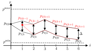
Figure 1: The illustration of scheduling tubes over the MPC prediction horizon, here $N=6$.

Furthermore, we assume that system (1) is subject to polytopic state and input constraints defined as

$$\mathbb{X} :=\{x_{k}\in\mathbb{R}^{n_{\rm x}}\mid G^{\rm x}x_{k}\leq h^{\rm x}\},$$ (6)

$$\mathbb{U} :=\{u_{k}\in\mathbb{R}^{n_{\rm u}}\mid G^{\rm u}u_{k}\leq h^{\rm u}\}.$$ (7)

where $G^{\rm x}\in\mathbb{R}^{p_{\rm x}\times n_{\rm x}}$, $h^{\rm x}\in\mathbb{R}^{p_{\rm x}}$, $G^{\rm u}\in\mathbb{R}^{p_{\rm u}\times n_{\rm u}}$ and $h^{\rm u}\in\mathbb{R}^{p_{\rm u}}$.

2.2 Lateral and Longitudinal Vehicle Dynamics

The continuous time lateral vehicle dynamics are defined using the lateral error model from (Rajamani, 2011, p. 36):

$$\!\!\!\!\!\!\!\!\frac{\text{d}}{\text{d}t}\!\!\begin{bmatrix}e^{\rm y}(t)\\ \dot{e}^{\rm y}(t)\\ e^{\psi}(t)\\ \dot{e}^{\psi}(t)\end{bmatrix}\!\!\!=\!\!\!\begin{bmatrix}0&1&0&0\\ 0&a&b&c\\ 0&0&0&1\\ 0&d&e&f\\ \end{bmatrix}\!\!\!\!\begin{bmatrix}e^{\rm y}(t)\\ \dot{e}^{\rm y}(t)\\ e^{\psi}(t)\\ \dot{e}^{\psi}(t)\end{bmatrix}\!\!+\!\!\begin{bmatrix}\!0\!\\ \!\frac{2C_{\alpha\rm f}}{m}\!\\ \!0\!\\ \!\frac{2C_{\alpha\rm f}l_{\rm f}}{I_{\rm z}}\!\\ \end{bmatrix}\!\!\delta(t)\!+f^{\psi}(t),$$ (8)

where $e^{\rm y}(t)$ and $e^{\psi}(t)$ are the distance of the center of gravity of the vehicle from the centerline of the lane and the orientation error of the vehicle with respect to the road, respectively, as demonstrated in Fig. 2. The states $\dot{e}^{\rm y}(t)$ and $\dot{e}^{\psi}(t)$ are the rate of change of $e^{\rm y}(t)$ and $e^{\psi}(t)$. The control input is the steering angle of the vehicle, i.e., $\delta(t)$. The function $f^{\psi}(t)$ is defined as

$$f^{\psi}(t)=\!\begin{bmatrix}0&g&0&h\end{bmatrix}^{\top}\dot{\psi}^{\rm{des}}(t),$$ (9)

where $\dot{\psi}^{\rm{des}}(t)$ denotes the yaw rate of the road. All the other parameters in (8) and (9) are described as follows:

$$\begin{split}a&=-\frac{2C_{\alpha\rm f}+2C_{\alpha\rm r}}{{m}v^{\rm x}(t)},\\ c&=\frac{-2C_{\alpha\rm f}l_{\rm f}+2C_{\alpha\rm r}l_{\rm r}}{{m}v^{\rm x}(t)},\\ e&=\frac{2C_{\alpha\rm f}l_{\rm f}-2C_{\alpha\rm r}l_{\rm r}}{I_{\rm z}},\\ g&=-\frac{2C_{\alpha\rm f}l_{\rm f}-2C_{\alpha\rm r}l_{\rm r}}{{m}v^{\rm x}(t)}\!-\!v^{\rm x}(t),\end{split}$$

$$\begin{split}b&=\frac{2C_{\alpha f}+2C_{\alpha\rm r}}{m},\\ d&=-\frac{2C_{\alpha f}l_{\rm f}-2C_{\alpha\rm r}l_{\rm r}}{I_{\rm z}v^{\rm x}(t)},\\ f&=-\frac{2C_{\alpha f}l^{2}_{\rm f}+2C_{\alpha\rm r}l^{2}_{\rm r}}{I_{\rm z}v^{\rm x}(t)},\\ h&=-\frac{2C_{\alpha f}l^{2}_{\rm f}+2C_{\alpha\rm r}l^{2}_{\rm r}}{I_{\rm z}v^{\rm x}(t)},\end{split}$$

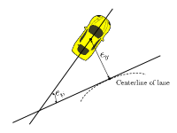
Figure 2: Notation of the vehicle (Carvalho et al. (2014))

with $v^{\rm x}(t)$ representing the longitudinal speed. The constant parameters used in the model, alongside their values and units, are explained in Table 1.

Symbol	Parameter	Value
$C_{\alpha\rm f}$	Cornering Stiffness Front	$153$ kN$/$rad
$C_{\alpha\rm r}$	Cornering Stiffness Rear	$191$  kN$/$rad
$l_{\rm f}$	Distance CoG to Front Axle	$1.3$  m
$l_{\rm r}$	Distance CoG to Rear Axle	$1.7$  m
$I_{\rm z}$	Vehicle Yaw Inertia	$5250$  kgm2
$m$	Vehicle Mass	$2500$ kg
${\rm l}^{\rm width}$	lane width	$10$ $\rm m$

Table 1: Vehicle parameters used in vehicle modeling (Gottmann et al. (2018))

Model (8) is discretized in time using the Euler discretization rule with a sampling time of $t_{s}$. Then, the resulted discrete-time model can be realized as an LPV model of the form (1), where $p_{k}=1/v^{\rm x}_{k}$, $x_{k}=\begin{bmatrix}e^{\rm y}_{k}&\Delta e^{\rm y}_{k}&e^{\psi}_{k}&\Delta e^{\psi}_{k}\end{bmatrix}^{\top}$, $u_{k}=\delta_{k}$, and $w_{k}=f^{\psi}_{k}$, where $k$ is the sampling index. The sets $\mathcal{P}$ and $\mathcal{W}$ can be directly defined by specifying the maximum and minimum values of $1/v^{\rm x}$ and $f^{\psi}$, respectively. It is assumed that $f^{\psi}(t)$ is bounded with known bounds based on the upper and lower bounds on the road curvature. We assume that the exact value of $f^{\psi}(t)$ is not measurable in advance. Therefore, $f^{\psi}(t)$ is considered as an additive uncertainty over the MPC prediction horizon, representing the term $w$ in (1).

The state and input constraints, i.e., $\mathbb{X}$ and $\mathbb{U}$, are defined as (6) and (7), respectively, where

$$G^{\rm x} =\begin{bmatrix}\mathbb{I}_{4\times 4}&-\mathbb{I}_{4\times 4}\end{bmatrix}^{\top},\qquad h^{\rm x}=\begin{bmatrix}h&h\end{bmatrix}^{\top},$$ (10)

with $h=\begin{bmatrix}e^{\rm y_{max}}&\Delta e^{\rm y_{max}}&e^{\psi_{\rm max}}&\Delta e^{\psi_{\rm max}}\end{bmatrix}^{\top}$ and

$$G^{\rm u} =\begin{bmatrix}1&-1\end{bmatrix}^{\top},\qquad h^{\rm u}=\begin{bmatrix}\delta^{\rm max}&\delta^{\rm max}\end{bmatrix}^{\top}.$$ (11)

Lane keeping is attained by satisfying the constraint on $e^{\rm y}_{k}$. In other words, by considering $e^{\rm y_{max}}=\frac{{\rm l}^{\rm width}}{2}-\frac{\rm w^{\rm vehicle}}{2}$, where ${\rm l}^{\rm width}$ is given in Table 1 and $\rm w^{\rm vehicle}$ is the width of the vehicle. Note that $e^{\rm y}_{k}=0$ means the vehicle is at the centerline of the lane.

Next, the continuous longitudinal dynamics of the vehicle are presented as follows:

$$\frac{\text{d}}{\text{d}t}\begin{bmatrix}s(t)\\ v^{\rm x}(t)\end{bmatrix}=\begin{bmatrix}0&1\\ 0&0\end{bmatrix}\!\begin{bmatrix}s(t)\\ v^{\rm x}(t)\end{bmatrix}+\begin{bmatrix}0\\ 1\\ \end{bmatrix}a(t),$$ (12)

where $s(t)$, $v^{\rm x}(t)$, and $a(t)$ denote the longitudinal position of the center of gravity, the longitudinal speed, and the longitudinal acceleration, respectively. System (12) is discretized using the Euler discretization method:

$$\begin{bmatrix}s_{k+1}\\ v^{\rm x}_{k+1}\end{bmatrix}=\begin{bmatrix}1&t_{s}\\ 0&1\end{bmatrix}\begin{bmatrix}s_{k}\\ v^{\rm x}_{k}\end{bmatrix}+\begin{bmatrix}0\\ t_{s}\end{bmatrix}a_{k},$$ (13)

where, $s_{k}$ and $v^{\rm x}_{k}$ are the discretized system states and $t_{s}$ is the sampling time. The longitudinal speed is bounded as $v^{\rm min}\leq v^{\rm x}_{k}\leq v^{\rm max}$. The acceleration is bounded as $a^{\rm min}\leq a_{k}\leq a^{\rm max}$.

3 Control Architecture and MPC Design

The proposed control architecture is depicted in Fig. 3. A speed planner generates desired reference values for the longitudinal speed of the vehicle. Then, a longitudinal MPC is used to generate the corresponding accelerations to reach the reference speeds while taking the longitudinal state and input constraints into account. Next, the generated speeds by the longitudinal dynamics are used to schedule the lateral MPC, as explained in the following.

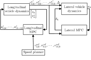
Figure 3: Depiction of the proposed control architecture

3.1 Longitudinal MPC

The following MPC is suggested as the controller for the longitudinal dynamics:

$$\underset{a_{0|k},\cdots,a_{N-1|k}}{\text{min}} \sum_{i=0}^{N-1}\eta(v^{\rm x}_{i+1|k}-v^{\rm ref}_{i+1|k})^{2}+\zeta a_{i|k}^{2}$$

s.t. $$\text{Eq.~{}\eqref{long_model_disc}},\quad\forall i=0,\cdots,N-1,$$

$$\begin{bmatrix}s_{0|k}&v^{\rm x}_{0|k}\end{bmatrix}^{\top}=\begin{bmatrix}s_{k}&v^{\rm x}_{k}\end{bmatrix}^{\top},$$

$$\begin{bmatrix}0&1\\ 0&-1\end{bmatrix}\!\!\begin{bmatrix}s_{i|k}\\ v^{\rm x}_{i|k}\end{bmatrix}\leq\begin{bmatrix}v^{\rm max}\\ -v^{\rm min}\end{bmatrix},$$

$$\begin{bmatrix}1\\ -1\end{bmatrix}a_{i|k}\leq\begin{bmatrix}a^{\rm max}\\ -a^{\rm min}\end{bmatrix},$$ (14)

where, $\eta>0$ and $\zeta>0$ are tuning constants. The current longitudinal state of the vehicle is denoted by $\begin{bmatrix}s_{k}&v^{\rm x}_{k}\end{bmatrix}^{\top}$.

3.2 Lateral MPC

The lateral MPC is designed to keep the vehicle in a lane. The prediction in such an LPV-MPC scheme is based on (1). In this problem, the initial conditions $x_{k}$, $p_{k}$ and $w_{k}$ are available for the MPC at any time instant $k$; however, the prediction of the state over the MPC prediction horizon, i.e., $x_{k+i}$ for $i=1,\cdots,N$, is a function of $u_{k+i-1}$, $p_{k+i}$ and $w_{k+i}$, which are not available in advance.

After generation of the accelerations $a^{*}_{0|k},\cdots,a^{*}_{N-1|k}$, by the longitudinal MPC, the future values $v^{\rm x^{*}}_{1|k},\cdots,v^{\rm x^{*}}_{N|k}$ can be computed and used to compute a future scheduling parameter, i.e., $p_{i|k}=1/v^{\rm x}_{i|k}$, over the prediction horizon of the lateral MPC. However, due to the physical constraints of the vehicle and inaccuracies of its model, the actual future vehicle speed might deviate slightly from what is generated by the longitudinal MPC. In order to take such uncertainty into account, we employ the available information about $v^{\rm x^{*}}_{1|k},\cdots,v^{\rm x^{*}}_{N|k}$ to compute nominal values of the future scheduling parameter, i.e., $\hat{p}_{i|k}$, and add a predefined uncertainty region $\Delta$ around such nominal future scheduling parameter, see (4), which leads to a scheduling tube as demonstrated in Fig. 1. In other words, at every time step $k$, the first value of the scheduling parameter $p_{0|k}=p_{k}$, which corresponds to the longitudinal speed of the vehicle $v^{\rm x}_{0|k}$, is considered to be exactly known. Whereas over the rest of the horizon, the bounded uncertainty $\Delta$ is considered around $\hat{p}_{i|k}$ to take into consideration the uncertainty of ${p}_{i|k}$. To handle the lateral MPC problem with such scheduling tubes, we adopt a modified formulation of the approach from the paper by Hanema et al. (2016) as follows.

Consider the following non-empty polytopic set as an invariant set for the LPV system (1):

$$\mathcal{S}=\{x_{k}\in\mathbb{R}^{n_{\rm x}}|G^{\rm f}x_{k}\leq h^{\rm f}\}.$$ (15)

Computation of $\mathcal{S}$ can be done offline and will be explained in the next section. A constraint invariant tube using homothetic cross section parameterization, (Raković et al. (2012)), is defined as follows:

$$X_{k}:=z_{k}\oplus\alpha_{k}\mathcal{S},$$ (16)

where $z_{k}\in\mathbb{R}^{n_{\rm x}}$ and $\alpha_{k}\in\mathbb{R}_{+}$ represent the center and the radius of the tube, respectively; $z_{k},\alpha_{k}$ are introduced as decision variables in the MPC optimization problem. Therefore, the lateral MPC is given as

$$\underset{d_{k}}{\text{min}} \quad V_{f}(z_{N|k},\alpha_{N|k})+\sum_{i=0}^{N-1}l(z_{i|k},\alpha_{i|k},g_{i|k})$$

s.t. $$\alpha_{0|k}=0,\quad z_{0|k}=x_{k},$$

$$\forall i=0,1,\cdots,N-1:$$

$$X_{i|k}=z_{i|k}\oplus\alpha_{i|k}\mathcal{S},$$

$$u_{i|k}=g_{i|k}\oplus\alpha_{i|k}\mathcal{R},$$

$$A(p_{i|k})X_{i|k}+Bu_{i|k}\subseteq z_{i+1|k}+\alpha_{i+1|k}\mathcal{S},$$

$$X_{i|k}\in\mathbb{X},$$

$$u_{i|k}\in\mathbb{U},$$

$$X_{N|k}\in\mathcal{S},$$ (17)

where, $p_{i|k}\in\hat{p}_{i|k}\oplus\Delta$. The decision variable is $d_{k}=\begin{bmatrix}\alpha_{0|k},\cdots,\alpha_{N|k},z_{0|k},\cdots,z_{N|k},g_{0|k},\cdots,g_{N-1|k}\end{bmatrix}^{\top}$.The input and state constraints $\mathbb{U}$ and $\mathbb{X}$ are defined in (11) and (10), respectively. The invariant set $\mathcal{S}$ as defined in (15) is used as the terminal set of the MPC and to parameterize the state tube to take into account the uncertainty of $p$ over $N$ and possible additive uncertainty, i.e., $w$, for the system (1). In the optimization problem (3.2), the set $\mathcal{R}$ is used to parameterize the control tube. The simplest way to compute $\mathcal{R}$ is $\mathcal{R}=K\mathcal{S}$, where $K$ is chosen such that $A(p_{k})+BK$, is stable for all $p_{k}\in\mathcal{P}$. However, the constant $K$ can lead to a very conservative solution for the LPV-MPC (3.2). Alternatively, choosing a parameter-dependent gain $K(p_{k})$ is preferred; see next section for more details. In this case, $\mathcal{R}$ in (3.2) also depends on time and can be computed as follows:

$$\mathcal{R}_{i|k}=K(p_{i|k})\mathcal{S},$$ (18)

for all $p_{i|k}\in\hat{p}_{i|k}\oplus\Delta$. The implementation of such formulation is explained in the next section. The cost function in the optimization problem (3.2) is still in terms of the uncertain state. A worst-case stage cost, based on Hanema et al. (2016), can be computed as

$$l(z_{i|k},\alpha_{i|k},g_{i|k})=\underset{(x,u)\in X_{i|k}\times\mathcal{R}}{\text{max}}\|x\|^{2}_{Q}+\|u\|^{2}_{R},$$ (19)

where $Q={Q}^{\top}\succ 0$ and $R={R}^{\top}\succ 0$ are the tuning matrices. The terminal cost in (3.2) can be computed as

$$V_{f}(z_{N|k},\alpha_{N|k})=\underset{x\in X_{N|k}}{\text{max}}\|x\|^{2}_{P},$$ (20)

where the terminal cost $P$ is a constant positive definite matrix $P=P^{\top}\succ 0$ satisfying the condition $(A(p)+BK)^{\top}P(A(p)+BK)-P\leq-({Q}+K^{\top}{R}K)$, for all $p\in\mathcal{P}$. Similar to what was just discussed for the computation of $\mathcal{R}$, a less conservative terminal cost is to consider $P$ parameter-dependent, i.e., $P(p)=P^{\top}(p)\succ 0$, $\forall p\in\mathcal{P}$ as explained in the next section. The main difference between the LPV-MPC scheme presented here and that in Hanema et al. (2016) is that the latter did not consider the additive term, i.e., $w_{k}=0,\forall k$. Also the paper considers contractive invariant sets. For this reason, the terminal cost in (20) is different from that in Hanema et al. (2016). For the stability of the control law generated by this LPV-MPC scheme and its recursive feasibility without additive disturbance, the reader can refer to Hanema et al. (2016), whereas these theoretical results cannot be guaranteed in the presence of additive disturbance. However, any infeasibility or instability have not been observed in the simulations.

4 Computation of the Invariant Set

Consider the LPV system (1), where $p_{k}\in\mathcal{P}$ is presented in (2). Using an LPV state feedback controller as follows

$$u_{k}=K(p_{k})x_{k},$$ (21)

system (1) is called poly-quadratically stabilized according to Pandey and de Oliveira (2017) if the linear matrix inequality (LMI) conditions shown below are satisfied.

Consider the vertex representation of the system matrix of (1) as $A(p_{k})=\textbf{Conv}(A^{1},A^{2},\cdots,A^{n_{\rm v}})$ where $A^{1}$, $A^{2}$, $\cdots$ are the evaluation of $A(p_{k})$ at the $n_{\rm v}$ vertices of the set $\mathcal{P}$. Then, $K(p_{k})$ can be computed by solving the following set of LMIs (Bao et al. (2022)):

$$\begin{bmatrix}X^{j}\!\!+\!\!{X^{j}}^{\top}\!\!\!-\!S^{j}&*&*&*&*\\ {A^{j}}^{\top}X^{j}&S^{l}\!-\!BY^{l}\!+\!{Y^{l}}^{\top}\!{B}^{\top}&*&*&*\\ -W^{j}&{Z^{l}}^{\top}{B}^{\top}-Y^{l}&Z^{l}\!\!+\!\!{Z^{l}}^{\top}&*&*\\ {Q}^{1/2}X^{j}&0&0&\mathbb{I}&*\\ {R}^{1/2}W^{j}&0&0&0&\mathbb{I}\end{bmatrix}\!\succ\!0,$$ (22)

for $j,l=1,2,\cdots,n_{\rm v}$ such that the matrices $X^{j},W^{j},Y^{j}$ and $S^{j}\succ 0$. Thus, the feedback gain is computed as $K^{j}=W^{j}{X^{j}}^{-1}$, where $K^{j}$ denotes the $j^{\rm th}$-vertex according to $K(p_{k})=\textbf{Conv}(K^{1},K^{2},\cdots,K^{n_{\rm v}})$. This yields the associated Lyapunov matrix $P$ parameter-dependent such that $P(p_{k})=\textbf{Conv}(P^{1},P^{2},\cdots,P^{n_{\rm v}})$ where $P^{j}={S^{j}}^{-1}$.

The usage of $P(p_{k})$ and $K(p_{k})$ after their computation by solving the LMI problem (22) is indicated in the next section.

Definition 4.1 (Robust positive invariant set)

The
set $\mathcal{S}\in\mathbb{X}$ is said to be a robust positively invariant (RPI) set for the system (1) with $u_{k}=K(p_{k})x_{k}\in\mathbb{U}$, if for all $p_{k}\in\mathcal{P}$ and all $w_{k}\in\mathcal{W}$, having $x_{k}\in\mathcal{S}$ leads to $x_{k+1}\in\mathcal{S}$ (Blanchini (1999)).

For the LPV lateral vehicle model, represented in the form (1), possible changes in the curvature of the road are considered as additive disturbances, which are considered in the computation of $\mathcal{S}$ given the set $\mathcal{W}$. Therefore, anytime the road profile changes, and consequently, the upper and lower bounds on the road curvature change, it means that the disturbance set has changed, then $\mathcal{S}$ has to be recomputed. Computation of $\mathcal{S}$ is performed offline.

5 Results and Discussions

5.1 Implementation

Let the set $\mathcal{S}$ be presented as:

$$\mathcal{S}=\textbf{Conv}(v^{1},v^{2}\cdots,v^{r}),$$ (23)

where $v^{1},v^{2}\cdots,v^{r}$ are the vertices of $\mathcal{S}$. Based on the vertices representation of $\mathcal{S}$, the optimization problem (3.2) can be implemented as follows:

$$\underset{d_{k}}{\text{min}} \sum_{j=1}^{r}\|z_{N|k}\oplus\alpha_{N|k}v^{j}\|^{2}_{P^{l}}$$

$$+\sum_{i=0}^{N-1}\sum_{j=1}^{r}\|z_{i|k}\oplus\alpha_{i|k}v^{j}\|^{2}_{Q}+\|g_{i|k}+\alpha_{i|k}K^{l}v^{j}\|^{2}_{R}$$

s.t. $$\alpha_{0|k}=0,\quad z_{0|k}=x_{k},$$

$$G^{\rm f}(z_{N|k}\oplus\alpha_{N|k}v^{j})\leq h^{\rm f},$$

$$G^{\rm f}(A(\overline{p}_{i|k})(z_{i|k}\!\oplus\!\alpha_{i|k}v^{j}\!)\!+\!B(g_{i|k}\!+\!\alpha_{i|k}K^{l}v^{j}))\!$$

$$\hskip 125.19212pt\leq\!G^{\rm f}z_{i+1|k}\!+\!\alpha_{i+1|k}h^{\rm f}\!,$$

$$G^{\rm f}(A(\underline{p}_{i|k})(z_{i|k}\!\oplus\!\alpha_{i|k}v^{j}\!)\!+\!B(g_{i|k}\!+\!\alpha_{i|k}K^{l}v^{j}))\!$$

$$\hskip 125.19212pt\leq\!G^{\rm f}z_{i+1|k}\!+\!\alpha_{i+1|k}h^{\rm f}\!,$$

$$G^{\rm x}(A(\overline{p}_{i|k})(z_{i|k}\!\oplus\!\alpha_{i|k}v^{j})\!+\!B(g_{i|k}\!+\!\alpha_{i|k}K^{l}v^{j}))\leq h^{\rm x},$$

$$G^{\rm x}(A(\underline{p}_{i|k})(z_{i|k}\!\oplus\!\alpha_{i|k}v^{j})\!+\!B(g_{i|k}\!+\!\alpha_{i|k}K^{l}v^{j}))\leq h^{\rm x},$$

$$G^{\rm u}(g_{i|k}+\alpha_{i|k}K^{l}v^{j})\leq h^{\rm u},$$ (24)

$$\forall i=0,1,\cdots,N\!-\!1,\quad\forall j=1,2,\cdots,r,\quad\forall l=1,2,$$

where $v^{j}$ are the vertices of $\mathcal{S}$ from (23), $j,l$ denote the vertex number of the sets $\mathcal{S}$ and $\mathcal{P}$, respectively. The parameters $K^{l}$ and $P^{l}$ are the vertices of LPV state feedback gain and the LPV terminal weight, calculated by solving the LMI problem (22). Note that, with one scheduling parameter for the LPV lateral model, the number of vertices of $\mathcal{P}$ is $n_{\rm v}=2$. The rest of the parameters are the same as for the optimization problem (3.2).

5.2 Simulation Results

An example of a lane keeping scenario by the proposed control architecture is illustrated in Fig. 4. The scenario is simulated using YALMIP (Löfberg (2004)) and solved by quadprog solver in MATLAB (2019). In this scenario, the vehicle is controlled to approach the centerline of the road using the proposed control architecture. The parameters used in the lateral and longitudinal MPC in this scenario are given in Table 2. The initial conditions are chosen as $e^{\rm y}_{0}=3.27$ $\rm m$, $\dot{e}^{\rm y}_{0}=0.55$ $\frac{\rm m}{\rm s}$, $e^{\psi}_{0}=-0.24$ $\rm rad$, $\dot{e}^{\psi}_{0}=0.3$ $\frac{\rm rad}{\rm s}$, $s_{0}=1$ $\rm m$ and $v^{\rm x}_{0}=25$ $\frac{\rm m}{\rm s}$.

For the computation of $\mathcal{S}$, at first, an LPV state feedback controller, as explained in Section 4, is designed. It has been observed that changing $Q$ and $R$ highly affects the number of vertices of $\mathcal{S}$, which has a great impact on the number of inequality constraints in the related MPC problem. Similar to the method presented by Nguyen et al. (2020), different values for $Q$ and $R$ have been tried. Among the test values, the values for $Q$ and $R$, which result in the least number of vertices for $\mathcal{S}$, have been selected as the final values. The final selected values for $Q$ and $R$ can be seen in Table 2. The set $\mathcal{S}$ is computed by using the algorithm for RPI set computation by (Nguyen, 2014, p. 25). This choice results in $93$ vertices for $\mathcal{S}$, which leads to 1770 inequality constraints when setting up the MPC.

Parameter	Value	Parameter	Value
$\eta$	$100$	$\zeta$	$0.1$
$a_{\rm min}$	$-6\frac{\rm m}{\rm s^{2}}$	$a_{\rm max}$	$2\frac{\rm m}{\rm s^{2}}$
$N$	$5$	$t_{s}$	$0.1$ s
$e^{\rm y_{max}}$	$4$m	$\Delta e^{\rm y_{\rm max}}$	$10\frac{\rm m}{\rm s}$
$e^{\psi_{\rm max}}$	$\frac{\rm pi}{2}$ rad	$\Delta e^{\psi_{\rm max}}$	$\frac{\rm pi}{3t_{s}}$ $\frac{\rm rad}{\rm s}$
$v^{\rm max}$	$30\frac{\rm m}{\rm s}$	$v^{\rm min}$	$15\frac{\rm m}{\rm s}$
$Q$	$50\mathbb{I}_{4\times 4}$	$R$	$5$
$\Delta$	$0.2$	$d^{\max}=-d^{\min}$	$10^{-2}\mathds{1}_{4\times 1}$

Table 2: The MPC parameters

The reference speed generated by the speed planner is assumed to be $18$ $\frac{\rm m}{\rm s}$. As illustrated in Figs. 5 and 6, the vehicle decelerates with the maximum value until its longitudinal speed reaches the reference value of $18$ $\frac{\rm m}{\rm s}$. The steering angles generated by the lateral MPC to bring the vehicle to the centerline of the road are demonstrated in Fig 7. In Fig. 8, the blue line indicates the nominal values of the scheduling parameter, i.e., $\hat{p}_{k}$, and the red line represents the actual values, i.e., $p_{k}$. The green tube around the blue line is plotted based on the value of $\Delta$, given in Table 2. In the simulations, the deviation of $p_{k}$ from its nominal value, based on the value of $\Delta$, is generated randomly.

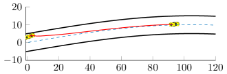
Figure 4: A sample lane keeping scenario

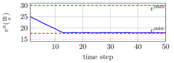
Figure 5: Longitudinal speed of the vehicle

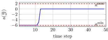
Figure 6: Longitudinal acceleration of the vehicle

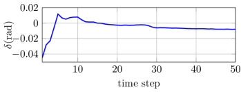
Figure 7: Steering angle

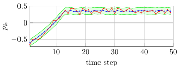
Figure 8: The scheduling parameter

As the sample scenario confirms, by using the proposed architecture, the vehicle can track the reference, while the state and input constraints are satisfied. Furthermore, the simulation results confirm that the lateral MPC is robust against changes in the scheduling parameter.

6 Conclusions

In this paper, the lateral dynamics of a vehicle with an additive term have been embedded in an LPV representation, where the speed of the vehicle is the scheduling parameter. A robust control architecture consisting of two subsequent controllers is proposed for lane keeping. At first, a longitudinal MPC for controlling the longitudinal dynamics has been employed. Then, the longitudinal MPC provides an estimate of the vehicle speed to be used by the subsequent MPC for controlling the lateral dynamics. For robustification of the lateral MPC, an uncertainty region around the estimated speeds (the scheduling parameter) has been considered. Still, there is a lot to be explored in this area. e.g., extending the work to obstacle avoidance scenarios or providing guarantees for stability and recursive feasibility.

References

- Abbas et al. (2018) Abbas, H.S., Hanema, J., Tóth, R., Mohammadpour, J., and Meskin, N. (2018). A new approach to robust mpc design for lpv systems in input-output form. IFAC-PapersOnLine, 51(26), 112–117.
- Alcalá et al. (2019) Alcalá, E., Puig, V., and Quevedo, J. (2019). Lpv-mpc control for autonomous vehicles. IFAC-PapersOnLine, 52(28), 106–113.
- Bao et al. (2022) Bao, Y., Abbas, H.S., and Velni, J.M. (2022). A learning-and scenario-based mpc design for nonlinear systems in lpv framework with safety and stability guarantees. arXiv preprint arXiv:2206.02880.
- Batkovic et al. (2020) Batkovic, I., Rosolia, U., Zanon, M., and Falcone, P. (2020). A robust scenario mpc approach for uncertain multi-modal obstacles. IEEE Control Systems Letters, 5(3), 947–952.
- Blanchini (1999) Blanchini, F. (1999). Set invariance in control. Automatica, 35(11), 1747–1767. 10.1016/s0005-1098(99)00113-2.
- Brüdigam et al. (2021) Brüdigam, T., Olbrich, M., Wollherr, D., and Leibold, M. (2021). Stochastic model predictive control with a safety guarantee for automated driving. IEEE Transactions on Intelligent Vehicles.
- Carvalho et al. (2014) Carvalho, A., Gao, Y., Lefevre, S., and Borrelli, F. (2014). Stochastic predictive control of autonomous vehicles in uncertain environments. In 12th International Symposium on Advanced Vehicle Control, 712–719.
- Gottmann et al. (2018) Gottmann, F., Wind, H., and Sawodny, O. (2018). On the influence of rear axle steering and modeling depth on a model based racing line generation for autonomous racing. In 2018 IEEE Conference on Control Technology and Applications (CCTA). IEEE. 10.1109/ccta.2018.8511508.
- Hanema et al. (2016) Hanema, J., Tóth, R., and Lazar, M. (2016). Tube-based anticipative model predictive control for linear parameter-varying systems. In 2016 IEEE 55th Conference on Decision and Control (CDC), 1458–1463. IEEE.
- Hashemi et al. (2012) Hashemi, S.M., Abbas, H.S., and Werner, H. (2012). Low-complexity linear parameter-varying modeling and control of a robotic manipulator. Control Engineering Practice, 20(3), 248–257.
- Heydari and Farrokhi (2021) Heydari, R. and Farrokhi, M. (2021). Robust tube-based model predictive control of lpv systems subject to adjustable additive disturbance set. Automatica, 129, 109672.
- Löfberg (2004) Löfberg, J. (2004). Yalmip : A toolbox for modeling and optimization in matlab. In In Proceedings of the CACSD Conference. Taipei, Taiwan.
- MATLAB (2019) MATLAB (2019). Version 9.6.0 (R2019a). The MathWorks Inc., Natick, Massachusetts, United States.
- Nezami et al. (2021) Nezami, M., Männel, G., Abbas, H.S., and Schildbach, G. (2021). A safe control architecture based on a model predictive control supervisor for autonomous driving. In 2021 European Control Conference (ECC), 1297–1302. IEEE.
- Nezami et al. (2022) Nezami, M., Nguyen, N.T., Männel, G., Abbas, H.S., and Schildbach, G. (2022). A safe control architecture based on robust model predictive control for autonomous driving. arXiv preprint arXiv:2206.09735.
- Nguyen (2014) Nguyen, H.N. (2014). Constrained Control of Uncertain, Time-Varying, Discrete-Time Systems. Springer International Publishing. 10.1007/978-3-319-02827-9.
- Nguyen et al. (2020) Nguyen, N.T., Prodan, I., and Lefèvre, L. (2020). Stability guarantees for translational thrust-propelled vehicles dynamics through nmpc designs. IEEE Transactions on Control Systems Technology, 29(1), 207–219.
- Pandey and de Oliveira (2017) Pandey, A. and de Oliveira, M.C. (2017). Quadratic and poly-quadratic discrete-time stabilizability of linear parameter-varying systems. IFAC-PapersOnLine, 50(1), 8624–8629.
- Rajamani (2011) Rajamani, R. (2011). Vehicle Dynamics and Control. Springer US. 10.1007/978-1-4614-1433-9.
- Raković et al. (2012) Raković, S.V., Kouvaritakis, B., Findeisen, R., and Cannon, M. (2012). Homothetic tube model predictive control. Automatica, 48(8), 1631–1638.
- Tearle et al. (2021) Tearle, B., Wabersich, K.P., Carron, A., and Zeilinger, M.N. (2021). A predictive safety filter for learning-based racing control. IEEE Robotics and Automation Letters, 6(4), 7635–7642.