Improving the Sample Efficiency of Prompt Tuning with Domain Adaptation

Abstract

Prompt tuning, or the conditioning of a frozen pretrained language model (PLM) with soft prompts learned from data, has demonstrated impressive performance on a wide range of NLP tasks. However, prompt tuning requires a large training dataset to be effective and is outperformed by finetuning the entire PLM in data-scarce regimes. Previous work Gu et al. (2022); Vu et al. (2022) proposed to transfer soft prompts pretrained on the source domain to the target domain. In this paper, we explore domain adaptation for prompt tuning, a problem setting where unlabeled data from the target domain are available during pretraining. We propose bOosting Prompt TunIng with doMain Adaptation (OPTIMA), which regularizes the decision boundary to be smooth around regions where source and target data distributions are similar. Extensive experiments demonstrate that OPTIMA significantly enhances the transferability and sample-efficiency of prompt tuning compared to strong baselines. Moreover, in few-shot settings, OPTIMA exceeds full-model tuning by a large margin.

1 Introduction

Prompt tuning (Lester et al., 2021; Li and Liang, 2021; Liu et al., 2022; Hambardzumyan et al., 2021) is an effective method for adapting large-scale pretrained language models for downstream tasks. While keeping the PLM weights unchanged, prompt tuning trains input vectors, called soft prompts, that are input to the PLM alongside the text embeddings. Compared to other adaptation techniques for PLMs, such as Adapter Houlsby et al. (2019); Rücklé et al. (2021); He et al. (2022), Compacter Mahabadi et al. (2021), BitFit Elad et al. (2022), LoRA Hu et al. (2021), and Ladder Side-Tuning Sung et al. (2022), the advantage of prompt tuning is that it does not require addition or change of model parameters. As a result, with prompt tuning, we can easily specialize one neural network (possibly deployed on a large number of servers or as application-specific integrated circuits) to support many different tasks by simply switching out the soft prompt in the input, which greatly simplifies model deployment and maintenance.

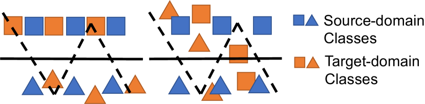
Figure 1: Smooth vs. zigzag decision boundaries. Left: When the distribution of the target-domain data (orange) are similar to the source domain (blue), the smooth decision boundary (solid line) generalizes better than the zigzag boundary. Right: When the distributions are different, it is not clear if the smooth decision boundary is the better choice.

However, training effective soft prompts usually requires sufficient labeled training data Su et al. (2021). Studies have shown that prompt tuning significantly underperforms full-model tuning on many few-shot classification tasks Gu et al. (2022). Our experiments corroborate this finding. In addition, we find that, in few-shot learning, prompt tuning is equally, if not more, sensitive to random seed choices compared to full-model tuning, despite having far fewer trainable parameters (§3.4). Gu et al. (2022) address this by transferring prompts learned from a source domain to the target domain with limited training data.

In this paper, we investigate a related but different scenario, unsupervised domain adaptation (UDA) Wang et al. (2019); Long et al. (2022), where unlabeled data from the target domain are available. Such situations are common when data are abundant but the labeling cost, including annotator recruitment, annotator training, and quality assurance, is high. Utilizing unlabeled examples can be an effective approach toward enhancing the data efficiency of prompt tuning.

We propose bOosting Prompt TunIng with doMain Adaptation (OPTIMA). Employing regularization from adversarial perturbation, OPTIMA learns a smooth decision boundary that passes through regions of low data density. In addition, recognizing that the feature distributions in the two domains may overlap only partially, we propose to focus the regularization to regions where the target-domain and source-domain data exhibit high similarity. We illustrate the intuition in Figure 1.

The popular Domain-adversarial Neural Network (DANN) technique Ganin et al. (2016) encourages the network to learn domain-invariant features and optimizes for both a domain-specific task loss and a domain discrimination loss. However, the two losses could compete against each other, leading to optimization difficulties Guo et al. (2021). Empirically, DANN exhibit low performance for prompt tuning. We hypothesize that the low capacity of prompts worsens the optimization problem. To solve this issue, in OPTIMA, we create input disturbance vectors that optimize for domain similarity, so that the prompt needs to optimize for only the task loss. The separation leads to excellent results.

Experiments shows that OPTIMA learns effective data representations that transfer well to the target domain under zero-shot and few-shot settings. OPTIMA outperforms eight baselines, including state-of-the-art transfer learning techniques such as SPOT (Vu et al., 2022). Our contributions include the following.

1. To our best knowledge, OPTIMA is the first domain adaptation technique for soft prompt tuning, which does not require any labeled data from the target domain. Empirical results show that the unlabeled data boost target-domain performance significantly.

2. Catering to partial overlaps of the data distributions, we propose a targeted regularization technique that encourages smooth decision boundaries only in the areas where the two domains are similar.

3. Through empirical evaluation, we show that OPTIMA outperforms state-of-the-art baselines, improves data efficiency significantly, and effectively addresses domain shifts. Code and data are available at https://github.com/guoxuxu/soft-prompt-transfer/tree/main/optima.

2 Domain Adaptation for Prompt Tuning

In this section, we first introduce prompt tuning for text classification. Then, we introduce how to enhance in-domain generalization performance of soft prompts by augmenting the input with virtual perturbations. Next, we propose how to optimize the perturbations to reduce the domain gap and obtain soft prompts with domain-invariant knowledge. Finally, we show how to use the soft prompts to boost few-shot learning in the target domain.

2.1 Preliminaries: Prompt Tuning

We start by introducing some notations. The input $\bm{x}$ is a sequence of $n$ token embeddings, $\bm{x}=\langle x_{1},\ldots,x_{n}\rangle$. The trainable soft prompt sequence $\bm{p}$ has $m$ embeddings, $\bm{p}=\langle p_{1},\ldots,p_{m}\rangle$. The manually designed hard prompt sequence $\bm{h}$ has $k$ token embeddings $\bm{h}=\langle h_{1},\ldots,h_{k}\rangle$. All embedding vectors have $d$ dimensions. The soft prompt and the hard prompt are both task-specific. The hard prompt text is usually a natural language description of the task, whereas the soft prompts do not correspond to any text and are trained directly using gradient descent.

For classification problems, we adopt the masked language modeling formulation, which aims to predict a predefined verbalizer token $y\in\mathcal{V}$ at a masked position in the input. For example, for binary classification, the words “yes” and “no” may be used as verbalizers that indicate positive and negative predictions, where we may define the label space as $\mathcal{Y}=\{\mathrm{yes},\mathrm{no}\}$. In encoder-only networks such as BERT Devlin et al. (2019), the output of the encoder is mapped to the label space $\mathcal{Y}$ via a projection head. In encoder-decoder networks like T5 (Raffel et al., 2020), the decoder is responsible for generating the verbalizer token.

We concatenate all sequences and the embedding of the [MASK] token, $e([\textrm{MASK}])$, to form the final input to the PLM: $\langle\bm{p};\bm{h};\bm{x};e[\textrm{MASK}]\rangle$. For simplicity, we use the function $f(\bm{x},\bm{p})$ to denote the PLM prediction at the masked position, which is a multinomial distribution over $\mathcal{Y}$. We adopt the the cross-entropy classification loss $\ell_{\text{xe}}$ with the ground-truth label $y\in\mathcal{Y}$.

$$\ell_{\text{xe}}(\bm{x},y,\bm{p})=-\mathrm{log}\ P(f(\bm{x},\bm{p})=y).$$ (1)

We optimize the soft prompt by minimizing the expected loss over the labeled training set, $\mathcal{D}$:

$$\bm{p}^{*}=\operatorname*{arg\,min}_{\bm{p}}\mathop{\mathbb{E}}_{(\bm{x},y)\in\mathcal{D}}\big{[}\ell_{\text{xe}}(\bm{x},y,\bm{p})\big{]}.$$ (2)

2.2 The OPTIMA Approach

We build OPTIMA off two intuitions regarding domain adaptation. First, as the target domain provides no direct supervision, it is easy to overfit to the source domain. Therefore, it is important to mitigate overfitting by regularizing the network to maintain a smooth decision boundary.

Under an adversarial learning framework, we seek a small perturbation $\bm{\delta}$ that, when added to the input, results in maximum change in the model prediction. After that, we optimize the model parameters to minimize the prediction change under the adversarially perturbed input. The overall result is a network whose output $f(\bm{x})$ changes little where a small change is added to the input $\bm{x}$. In the sense of Lipschitz continuity, such a decision boundary is smooth. Smooth decision boundaries can be understood as passing through regions of low data density and are shown to improve generalization (Huang et al., 2020; Cicek and Soatto, 2019; Kim et al., 2019).

The second intuition is that we do not have to regularize the entire decision boundary. As the source and target domains may have different data distributions, all that matters is the decision boundary segment close to the target-domain data. Therefore, we target the regularization and the perturbation $\bm{\delta}$ to areas on the data manifold where the source domain and target domain are similar.

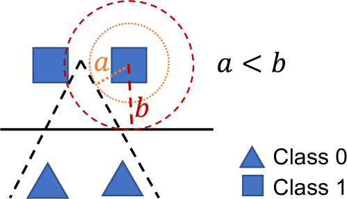
Figure 2: Intuition about perturbation and smoothness. Under the zigzag (non-smooth) decision boundary, a small perturbation with a well-chosen direction is sufficient to flip the predicted class. The smooth boundary requires a larger perturbation.

Specifically, we have a labeled dataset from the source domain, $\mathcal{D}_{s}=\{(\bm{x}_{s}^{(i)},y_{s}^{(i)})\}_{i=1}^{N_{s}}$, drawn i.i.d. from distribution $P_{s}$ and an unlabeled dataset from the target domain, $\mathcal{D}_{t}=\{\bm{x}_{t}^{(j)}\}_{j=1}^{N_{t}}$, drawn i.i.d. from distribution $P_{t}$. We define $\ell_{\text{KL}}$ as the KL divergence between the prediction of the original input and that of the perturbed input,

$$\ell_{\text{KL}}(\bm{\delta},\bm{p},\bm{x}_{s})=\mathrm{KL}(f(\bm{x}_{s},\bm{p})\;\|\;f(\bm{x}_{s}+\bm{\delta},\bm{p})).$$ (3)

$\ell_{\text{KL}}$ measures how much the model prediction changes when the perturbation $\bm{\delta}$ is applied to $\bm{x}_{s}$ and captures the smoothness of the decision boundary. We illustrate the intuition in Figure 2.

Further, we introduce a domain discriminator network parameterized by $\bm{\theta}_{d}$, which attempts to distinguish data instances from the two domains. This network is trained to reduce the domain discrimination loss $\mathcal{L}_{\text{disc}}$,

$$\mathcal{L}_{\text{disc}}(\bm{\delta},\bm{x}_{s},\bm{x}_{t})= \mathop{\mathbb{E}}_{\bm{x}_{s},\bm{x}_{t}}\big{[}-\mathrm{log}\ P(z=1|\bm{x}_{s}+\bm{\delta})$$

$$-\mathrm{log}\ P(z=1|\bm{x}_{s})$$ (4)

$$-\mathrm{log}\ P(z=0|\bm{x}_{t})\big{]},$$

where $z$ is the output of the discriminator network. This loss is a variation of the cross entropy with an additional term where $\bm{x}_{s}$ is perturbed by $\bm{\delta}$. In addition, we define an adversarial loss,

$$\ell_{\text{adv}}(\bm{\delta},\bm{x}_{s})=-\mathrm{log}\ P(z=1|\bm{x}_{s}+\bm{\delta}),$$ (5)

which, when maximized, causes the domain discriminator to mistake the perturbed source example $\bm{x}_{s}+\bm{\delta}$ as coming from the target domain.

For a given source-domain input, $\bm{x}_{s}$, we find the perturbation $\bm{\delta}^{*}$ within a $\epsilon$-radius ball that maximizes the following objective,

$$\bm{\delta}^{*}=\operatorname*{arg\,max}_{\bm{\delta},\|\bm{\delta}\|_{2}\leq\epsilon}\ell_{\text{KL}}(\bm{\delta},\bm{p},\bm{x}_{s})+\ell_{\text{adv}}(\bm{\delta},\bm{x}_{s}).$$ (6)

Here, $\ell_{\text{adv}}(\bm{\delta},\bm{x}_{s})$ can be understood as a regularization term for $\bm{\delta}$. By maximizing $\ell_{\text{KL}}$, we seek a disturbance to the input that causes the most change in the model prediction. At the same time, the disturbed input $\bm{x}_{s}+\bm{\delta}^{*}$ from the source domain should resemble data in the target domain, in order to maximize $\ell_{\text{adv}}(\bm{\delta},\bm{x}_{s})$; $\ell_{\text{adv}}$ constrains $\bm{\delta}^{*}$ to the region where the data from the two domains are similar.

We optimize the above loss w.r.t. $\bm{\delta}$ using projected gradient ascent (PGA). After every gradient descent step, $\bm{\delta}$ is projected back to the $\epsilon$-radius ball $\mathcal{Q}_{\epsilon}=\{\bm{\delta}|\|\bm{\delta}\|_{2}\leq\epsilon\}$. We write the projection operation as

$$\prod_{\|\cdot\|_{2}\leq\epsilon}(\bm{\phi})=\operatorname*{arg\,min}_{\bm{\delta}\in\mathcal{Q}_{\epsilon}}\|\bm{\delta}-\bm{\phi}\|_{2}=\frac{\epsilon\bm{\phi}}{\max(\epsilon,\|\bm{\phi}\|_{2})}.$$ (7)

The update to $\bm{\delta}$ can be written as

$$\bm{\delta} \leftarrow\prod_{\|\cdot\|_{2}\leq\epsilon}\left(\bm{\delta}+\eta_{\delta}\frac{\bm{g}}{\lVert\bm{g}\rVert_{2}}\right),$$ (8)

$$\bm{g} =\bigtriangledown_{\bm{\delta}}(\ell_{\text{KL}}(\bm{\delta},\bm{p},\bm{x}_{s})+\ell_{\text{adv}}(\bm{\delta},\bm{x}_{s})),$$ (9)

where $\eta_{\delta}$ is the learning rate. We normalize $\bm{g}$ to make sure the updates have the same magnitude.

During the training session, we alternately optimize the perturbation $\bm{\delta}$ and the soft prompt $\bm{p}$. With $\bm{\delta}^{*}$ found by PGA, we optimize the following loss function over $\bm{p}$ using standard gradient-based optimization.

$$\mathcal{L}_{R} =\mathop{\mathbb{E}}_{(\bm{x}_{s},y_{s})\in\mathcal{D}_{s}}\big{[}\ell_{\text{xe}}(\bm{x}_{s},y_{s},\bm{p})+\ell_{\text{KL}}(\bm{\delta}^{*},\bm{p},\bm{x}_{s})\big{]}$$

$$\bm{p}^{*} =\operatorname*{arg\,min}_{\bm{p}}\mathcal{L}_{R}$$ (10)

$\mathcal{L}_{R}$ is the empirical expectation computed over the current mini-batch. With the same $\bm{\delta}^{*}$, we also minimize the domain discrimination loss over the discriminator network parameter $\bm{\theta}_{d}$.

2.3 The OPTIMA Algorithm

We show the complete OPTIMA algorithm as Algorithm 1. With lines 5 and 6, we create an initial perturbation $\bm{\delta}_{0}^{(i)}$ for every source data point $\bm{x}_{s}^{(i)}$. From line 7 to line 13, we iteratively update the perturbation $\bm{\delta}^{(i)}$ associated with every source-domain data point $\bm{x}_{s}^{(i)}$ using projected gradient ascent on $\ell_{\text{KL}}+\ell_{\text{adv}}$. After $K$ iterations, we find $\bm{\delta}^{(i)}*=\bm{\delta}^{(i)}_{K}$, compute $\bigtriangledown_{\bm{p}}\mathcal{L}_{R}$ accordingly, and update $\bm{p}$ with stochastic gradient descent (SGD) and learning rate $\eta_{p}$ (line 16). At line 17, we update the domain discriminator parameters $\bm{\theta}_{d}$ using SGD with the current mini-batches. Though we show the vanilla SGD updates in lines 16-17, we can easily switch to other optimizers such as SGD with momentum or Adam (Kingma and Ba, 2015).

Input: A labeled source-domain dataset $\mathcal{D}_{s}=\{(\bm{x}_{s}^{(i)}y_{s}^{(i)})\}_{i=1}^{N_{s}}$ and an unlabeled target-domain dataset $\mathcal{D}_{t}=\{\bm{x}_{t}^{(j)}\}_{j=1}^{N_{t}}$, perturbation ball radius $\epsilon$, ascent steps $K$ and step size $\eta_{\delta}$.

Initialize: Soft prompts embeddings $\bm{p}$ and domain discriminator $\theta_{d}$, learning rates $\eta_{p},\eta_{d}$.

1

2repeat

3      

4      Sample a pair of batches, each of $B$ data points, from $\mathcal{D}_{s}$ and $\mathcal{D}_{t}$;

5       for $i=0,...,B$ do

6             Forward computation: $f(\bm{x}_{s}^{(i)},\bm{p}),\;\forall\bm{x}_{s}^{(i)}$

7             Sample a $\bm{\delta}_{0}^{(i)}\sim\mathcal{U}(-1,1)$, $\forall\bm{x}_{s}^{(i)}$

8             $\bm{\delta}_{0}^{(i)}\leftarrow\prod_{\|\cdot\|_{2}\leq\epsilon}(\bm{\delta}_{0}^{(i)})$

9             for $t=0,...,K-1$ do

10                   Forward with $\bm{\delta}_{t}^{(i)}$: $f(\bm{x}_{s}^{(i)}+\bm{\delta}_{t},\bm{p})$

11                   Compute $\ell_{\text{KL}}(\bm{\delta}_{t}^{(i)},\bm{p})$ (Eq. 3)

12                   Compute $\ell_{\text{adv}}(\bm{\delta}_{t}^{(i)})$ (Eq. 5)

13                   Perform PGA on $\bm{\delta}_{t}^{(i)}$:

14                   $\,\,\,\,\bm{g}\leftarrow\bigtriangledown_{\bm{\delta}_{t}^{(i)}}(\ell_{\text{KL}}(\bm{\delta}_{t}^{(i)},\bm{p})+\ell_{\text{disc}}(\bm{\delta}_{t}^{(i)}))$

15                   $\,\,\,\,\bm{\delta}_{t+1}^{(i)}\leftarrow\prod_{\|\cdot\|_{2}\leq\epsilon}(\bm{\delta}_{t}^{(i)}+\eta_{\delta}\cdot\frac{\bm{g}}{\|\bm{g}\|_{2}})$

16                  

17             end for

18            

19       end for

20      Compute $\mathcal{L}_{R}$ (Eq. 10), $\mathcal{L}_{\text{disc}}$ (Eq. 4) with $\bm{\delta}_{K}$

21       $\bm{p}\leftarrow\bm{p}-\eta_{p}\bigtriangledown_{\bm{p}}\mathcal{L}_{R}(\bm{x}_{s},y_{s},\bm{p})$

22       $\bm{\theta}_{d}\leftarrow\bm{\theta}_{d}-\eta_{d}\bigtriangledown_{\bm{\theta}_{d}}\mathcal{L}_{\text{disc}}(\bm{\delta}_{K},\bm{x}_{s},\bm{x}_{t};\bm{\theta}_{d})$

23      

24until the maximum training epoch is reached;

Output: Learned soft prompt $\bm{p}$

Algorithm 1 OPTIMA

2.4 Comparison with Virtual Adversarial Training

Virtual Adversarial Training (VAT) Miyato et al. (2016, 2018) is a pioneering work that applies adversarial perturbation to unlabeled examples in semi-supervised learning (SSL). The SSL assumption is that we have labeled data $(\bm{x},y)\overset{\mathrm{i.i.d.}}{\sim}P$ and unlabeled data $\bm{x}\overset{\mathrm{i.i.d.}}{\sim}P$. Notice that $\bm{x}$ is drawn from the same distribution $P$ regardless of the existence of the label $y$. VAT finds disturbance $\bm{\delta}\in\mathcal{Q}_{\epsilon}$ that maximizes the change in the model prediction $\mathrm{KL}(f(\bm{x})\;\|\;f(\bm{x}+\bm{\delta}))$. After that, the neural network minimizes cross-entropy on labeled data and the KL-divergence under disturbance on all data. Similar ideas have been explored in Cicek and Soatto (2019); Kim et al. (2019); Park et al. (2022).

A critical difference between SSL and domain adaptation is that the unlabeled data are drawn from a different distribution ($P_{t}$) than the labeled data ($P_{s}$). As the two distributions may overlap in some regions and diverge in others, regularizing over the the entire source dataset may be ineffective. Thus, we propose to focus the smoothness constraint on the regions of the data manifold where the source-domain and target-domain data are similar.

3 Experimental Evaluation

We evaluate the representations learned by OPTIMA under zero-shot and few-shot settings.

Dataset	Train	Test	$n_{class}$	Verbalizers
MRPC	4,076	408	2	Yes/No
QQP	363,847	40,430	2	Yes/No
MNLI	392,702	9,815	3	Yes/Neutral/No
SNLI	549,367	9,842	3	Yes/Neutral/No
SICK	4,439	4,906	3	Yes/Neutral/No
CB	250	56	3	Yes/Neutral/No

Table 1: Dataset characteristics.

Paraphrase	NLI from MNLI	NLI from SNLI
MRPC $\rightarrow$ QQP	MNLI $\rightarrow$ SNLI	SNLI $\rightarrow$ MNLI
QQP$\rightarrow$ MRPC	MNLI $\rightarrow$ SICK	SNLI $\rightarrow$ SICK
	MNLI $\rightarrow$ CB	SNLI $\rightarrow$ CB

Table 2: The set of domain adaptation experiments.

3.1 Datasets

We investigate domain adaptation on six text classification datasets in two tasks. In the task of paraphrase detection, we employ MRPC and QQP. In the task of natural language inference, we employ four datasets, including MNLI (Williams et al., 2018), SNLI (Bowman et al., 2015), CB (De Marneffe et al., 2019) and SICK (Marelli et al., 2014). The statistics and the label space $\mathcal{Y}$ of each dataset can be found in Table 1. We prepare 8 groups of cross-domain experiments, two for paraphrase detection and 6 for natural language inference (NLI), as shown in Table 2.

3.2 Baseline Techniques

We include eight competitive single-domain and cross-domain baselines. Out of the eight, baselines #2-#4 do not use any transfer learning from the source domain. Baselines #5-#9 utilize transfer learning and data from the source domain.

1) Frozen PLM. Large PLMs have demonstrated non-trivial zero-shot performance Brown et al. (2020). Here, we directly apply T5-large Raffel et al. (2020) with the manually written hard prompt and take the verbalizer with the highest probability as the prediction.

2) Prompt Tuning (PT). We feed the input data with both soft and hard prompts to a frozen T5-large model and finetune the soft prompt embeddings on the few-shot training set from the target domain.

3) Fine Tuning (FT). We feed the input data with the hard prompt to T5-large and finetune the entire network on the few-shot target-domain data. Notice that we use the verbalizer rather than training a separate task-specific prediction head.

4) Prompt-based Fine Tuning (PFT). A representative method on exploiting soft prompts for fine-tuning, e.g., PERFECT (Rabeeh et al., 2022). For fair comparison, we wrap the input with both soft and hard prompts and finetune both the PLM and the soft prompts on target-domain data. The predictions are mapped via verbalizers.

5) Pre-trained Prompt Tuning (PPT). We follow Gu et al. (2022), who propose to transfer to sentence-pair classification tasks by pretraining on the next sentence prediction task with 10GB text from OpenWebText (Gokaslan and Cohen, 2019). We download the pretrained checkpoint and finetune the soft prompt on the target domain directly.

6) Soft Prompt Transfer (SPOT). Vu et al. (2022) propose to pretrain soft prompts on source-domain datasets and finetune the learned soft prompts on the target-domain datasets. We apply this approach on different source-target pairs in few-shot setting.

7) Prompt Tuning with FreeLB. FreeLB (Zhu et al., 2020) is an adversarial training approach, which generates the adversarial perturbation from the supervised classification loss,

$$\bm{\delta}^{*}=\operatorname*{arg\,max}_{\bm{\delta},\|\bm{\delta}\|\leq\epsilon}\ell_{\text{xe}}(\bm{x}_{s}+\bm{\delta},y_{s},\bm{p}).$$ (11)

After that, we find the optimal $\bm{p}$ by minimizing $\ell_{\text{xe}}(\bm{x}_{s},y_{s},\bm{p})+\ell_{\text{xe}}(\bm{x}_{s}+\bm{\delta},y_{s},\bm{p})$. The adversarial training may be understood as another type of smoothness constraint, as the network attempts to maintain the same prediction despite the strongest possible perturbation.

8) Prompt Tuning with VAT. We apply the original VAT (Miyato et al., 2018) to generate the perturbations that maximally alter model predictions on the source domain,

$$\bm{\delta}^{*} =\operatorname*{arg\,max}_{\bm{\delta},\|\bm{\delta}\|\leq\epsilon}\ell_{\text{KL}}(\bm{\delta},\bm{p},\bm{x}_{s}),$$ (12)

and optimize $\bm{p}$ as in Equation 10. This can be seen as an ablation of OPTIMA, as Equation 12 omits the $\ell_{\text{adv}}$ term from Equation 6.

9) Prompt Tuning with DANN. We implement Domain-adversarial Neural Network (DANN) Ganin et al. (2016), a popular UDA method for prompt tuning. DANN introduces a domain discrimination loss $\mathcal{L}_{\text{DD}}$,

$$\mathcal{L}_{\text{DD}}=\mathop{\mathbb{E}}_{\bm{x}_{s},\bm{x}_{t}}\big{[} -\mathrm{log}\ P(z=1|\bm{x}_{s},\bm{p})$$ (13)

$$-\mathrm{log}\ P(z=0|\bm{x}_{t},\bm{p})\big{]},$$

where $z$ is the output of a domain discrimination network. The soft prompt $\bm{p}$ optimizes for the source-domain cross-entropy loss and the negative domain discrimination loss.

$$\bm{p}^{*}=\operatorname*{arg\,min}_{\bm{p}}\mathop{\mathbb{E}}_{(\bm{x}_{s},y_{s})\in\mathcal{D}_{s}}\big{[}\ell_{\text{xe}}(\bm{x}_{s},y_{s},\bm{p})\big{]}-\mathcal{L}_{\text{DD}}$$ (14)

For fair comparison, we use the same architecture for the domain discriminator as OPTIMA. Note that in DANN, the gradients from domain discrimination loss are backpropagated to the soft prompts, while in OPTIMA such gradients are backpropagated to the perturbations.

Method	Params	PLM	Source	QQP		MRPC		MNLI
				Acc.	F1	Acc.	F1	Acc.
Frozen	0	T5-Large	✗	45.5	54.9	33.8	11.8	41.7
PT	102K		✗	48.4 $\pm$ 4.9	52.5 $\pm$ 5.5	53.1 $\pm$ 11.4	55.9 $\pm$ 23.4	33.4 $\pm$ 1.6
FT	770M		✗	55.1 $\pm$ 6.7	52.0 $\pm$ 6.0	59.5 $\pm$ 7.8	67.9 $\pm$ 12.6	35.6 $\pm$ 2.4
PFT	770M		✗	55.1 $\pm$ 5.1	57.8 $\pm$ 3.1	58.9 $\pm$ 11.0	65.3 $\pm$ 11.8	35.6 $\pm$ 3.6
PPT	410K	T5-XXL	✓	52.1 $\pm$ 11.1	56.2 $\pm$ 21.1	52.1 $\pm$ 11.1	56.2 $\pm$ 21.1	34.4 $\pm$ 1.4
				MRPC $\to$ QQP		QQP $\to$ MRPC		SNLI $\to$ MNLI
				Acc.	F1	Acc.	F1	Acc.
SPOT	102K	T5-Large	✓	64.5 $\pm$ 2.7	64.5 $\pm$ 0.8	68.7 $\pm$ 2.5	77.1 $\pm$ 2.9	74.3 $\pm$ 0.9
FreeLB	102K		✓	65.0 $\pm$ 2.4	64.5 $\pm$ 1.5	68.5 $\pm$ 2.2	77.6 $\pm$ 2.2	75.0 $\pm$ 1.0
VAT	102K		✓	66.2 $\pm$ 2.0	64.9 $\pm$ 0.7	69.6 $\pm$ 1.9	79.0 $\pm$ 2.1	74.9 $\pm$ 1.1
DANN	102K		✓	63.4 $\pm$ 2.5	62.5 $\pm$ 2.7	68.0 $\pm$ 3.5	76.2 $\pm$ 5.1	73.1 $\pm$ 1.4
OPTIMA	102K		✓	69.1* $\pm$ 1.7	65.8* $\pm$ 1.9	71.2* $\pm$ 1.7	79.9* $\pm$ 1.7	78.4* $\pm$ 0.6
Method	Params	PLM	Source	SNLI	SICK		CB
				Acc.	Acc.		Acc.
Frozen	0	T5-Large	✗	35.9	37.1		55.4
PT	102K		✗	34.6 $\pm$ 2.4	61.5 $\pm$ 7.8		38.3 $\pm$ 13.6
FT	770M		✗	41.6 $\pm$ 3.8	67.6 $\pm$ 6.3		51.2 $\pm$ 7.8
PFT	770M		✗	38.6 $\pm$ 5.1	71.3 $\pm$ 6.4		57.3 $\pm$ 9.2
PPT	410K	T5-XXL	✓	34.7 $\pm$ 2.8	54.6 $\pm$ 14.0		43.0 $\pm$ 14.6
				MNLI $\to$ SNLI	SNLI $\to$ SICK	MNLI $\to$ SICK	SNLI $\to$ CB	MNLI $\to$ CB
				Acc.	Acc.	Acc.	Acc.	Acc.
SPOT	102K	T5-Large	✓	78.8 $\pm$ 1.1	69.9 $\pm$ 5.3	72.9 $\pm$ 5.9	61.7 $\pm$ 5.0	65.3 $\pm$ 3.4
FreeLB	102K		✓	81.5 $\pm$ 0.7	69.5 $\pm$ 6.8	73.1 $\pm$ 4.8	61.6 $\pm$ 4.2	66.1 $\pm$ 3.3
VAT	102K		✓	80.9 $\pm$ 0.9	68.6 $\pm$ 6.4	72.7 $\pm$ 6.3	59.0 $\pm$ 5.5	68.7 $\pm$ 4.8
DANN	102K		✓	71.1 $\pm$ 3.2	69.0 $\pm$ 6.7	73.4 $\pm$ 3.7	55.7 $\pm$ 5.5	66.9 $\pm$ 4.6
OPTIMA	102K		✓	82.1* $\pm$ 0.8	73.3 $\pm$ 6.8	74.8 $\pm$ 4.4	64.8* $\pm$ 1.1	71.2* $\pm$ 3.1

Table 3: Few-shot test performance. Results in bold are the best and results underlined are the best in the single-domain group. Results marked with * are significantly better than all the others under the student t-test ($p<0.05$).

3.3 Experiment Settings

Pretraining. For all methods that utilize source domain data, we train the soft prompts using the whole source-domain training set and perform model selection using the source-domain validation set. When domain adaptation is applied, we additionally use the entire target-domain training set for training with all labels removed. To mitigate variance, we train each method using 3 different random seeds, yielding three different models. For zero-shot evaluation, we report the mean score and standard deviation of the three models.

Few-shot Evaluation. Following Gao et al. (2021), we sample the few-shot training set and validation set from the original target training set. Each set contains 8 data points per class. We evaluate the trained model on the original target validation set. To mitigate high variance of few-shot learning, we repeat the sampling 16 times, and report the average of 48 runs (16 samples $\times$ 3 models). More details can be found in Appendix A.

Model Settings. For all the experiments, unless specified, we use the LM-adapted version of T5-large as the PLM. Results in Lester et al. (2021) (Figure 3) shows that T5 further trained for LM Adaptation works the best for prompt tuning, which is also adopted by Gu et al. (2022) and Vu et al. (2022). For the domain discriminator, we use a linear classification layer with parameters $\theta_{d}=[\bm{w},\bm{b}],\bm{w}\in\mathbb{R}^{1024\times 2},\bm{b}\in\mathbb{R}^{2}$, where $1024$ is the dimension of the output hidden states from the decoder of T5-large model.

Soft and Hard Prompts. Following Lester et al. (2021); Gu et al. (2022), for all methods other than PPT, we set the soft prompt length to 100, initialized to the first 100 alphabetic token embeddings of T5. We combine soft prompts with hard prompts with details in the Appendix A.

Evaluation Metrics. Following (Lester et al., 2021), we use accuracy and F1 score to evaluate the performance on the MRPC and QQP datasets. Following (Gu et al., 2022), we use accuracy for NLI. For zero-shot model selection, we use the source-domain validation set. For few-shot model selection, we use the target-domain validation set.

Method	MRPC	MRPC $\to$ QQP		QQP	QQP $\to$ MRPC		MNLI $\to$ CB
	Acc.	Acc.	F1	Acc.	Acc.	F1	Acc.
SPOT	82.5 $\pm$ 1.5	60.9 $\pm$ 4.6	63.6 $\pm$ 2.0	80.9 $\pm$ 2.2	65.7 $\pm$ 3.4	73.2 $\pm$ 5.7	63.2 $\pm$ 5.7
FreeLB	85.5 $\pm$ 0.3	63.1 $\pm$ 3.7	63.9 $\pm$ 1.0	82.2 $\pm$ 2.7	69.4 $\pm$ 1.1	78.7 $\pm$ 1.3	67.8 $\pm$ 3.9
VAT	84.7 $\pm$ 0.8	64.8 $\pm$ 4.6	64.1 $\pm$ 1.7	81.9 $\pm$ 0.7	68.9 $\pm$ 1.5	78.5 $\pm$ 1.5	67.8 $\pm$ 5.8
DANN	81.5 $\pm$ 2.1	63.9 $\pm$ 1.8	57.6 $\pm$ 3.3	81.4 $\pm$ 0.7	63.6 $\pm$ 4.8	71.5 $\pm$ 9.7	59.8 $\pm$ 4.4
OPTIMA	85.7 $\pm$ 0.7	68.9 $\pm$ 0.8	66.3 $\pm$ 0.6	82.7 $\pm$ 1.3	71.2 $\pm$ 0.4	80.0 $\pm$ 0.6	68.3 $\pm$ 2.6
Method	MNLI	MNLI $\to$ SNLI	MNLI $\to$ SICK	SNLI	SNLI $\to$ MNLI	SNLI $\to$ SICK	SNLI $\to$ CB
	Acc.	Acc.	Acc.	Acc.	Acc.	Acc.	Acc.
SPOT	83.4 $\pm$ 0.8	79.2 $\pm$ 1.0	51.8 $\pm$ 0.7	88.9 $\pm$ 0.1	75.6 $\pm$ 0.4	52.7 $\pm$ 1.9	47.6 $\pm$ 3.7
FreeLB	84.8 $\pm$ 0.8	81.8 $\pm$ 0.7	52.2 $\pm$ 0.2	89.9 $\pm$ 0.1	77.5 $\pm$ 0.5	52.9 $\pm$ 1.9	47.5 $\pm$ 4.7
VAT	83.7 $\pm$ 0.3	81.0 $\pm$ 0.2	51.4 $\pm$ 1.4	88.7 $\pm$ 0.1	77.1 $\pm$ 1.3	51.8 $\pm$ 2.1	45.8 $\pm$ 0.8
DANN	80.4 $\pm$ 2.7	72.4 $\pm$ 5.9	61.9 $\pm$ 2.7	85.3 $\pm$ 3.2	70.3 $\pm$ 3.6	51.5 $\pm$ 1.2	42.3 $\pm$ 2.2
OPTIMA	84.6 $\pm$ 0.3	82.1 $\pm$ 0.8	55.2 $\pm$ 1.0	89.2 $\pm$ 0.1	79.1 $\pm$ 0.1	53.8 $\pm$ 0.5	49.4 $\pm$ 4.2

Table 4: Source-domain and zero-shot target-domain test performance.

3.4 Few-shot Performance

We adopt few-shot classification to evaluate the representations learned by different models and pretraining methods. We show the few-shot performance in Table 3 and make the following observations. First, OPTIMA significantly outperforms all baseline models across all the few-shot test cases, including the state-of-the-art SPOT baseline. We perform statistical significance tests that compare OPTIMA to all baselines in a pair-wise manner. In all but the SICK experiments, the differences between OPTIMA and all baselines are statistically significant. We attribute the performance to the high-quality representation of OPTIMA, resulting from domain adaptation.

Second, DANN performs much worse than perturbation-based methods. As discussed earlier, we suspect the poor performance of DANN is partially due to the limited capacity of prompts (102K parameters in our case). In OPTIMA, the perturbation optimizes for domain invariance (Eq. 6), whereas the prompt optimizes for only task-specific losses (Eq. 10), which simplifies optimization for soft prompts.

Third, OPTIMA outperforms the VAT baseline, especially in the NLI tasks, where the performance difference ranges from 1.2% in MNLI$\rightarrow$SNLI to 5.8% in SNLI$\rightarrow$CB. The VAT baseline is an ablation of OPTIMA and omits the targeted regularization term when finding the perturbation. This comparison demonstrates the effectiveness of the proposed targeted smoothness constraint.

Finally, our experiments are consistent with earlier results of Gu et al. (2022), which show that prompt tuning (PT) suffers from high variance in the results. In the single-domain experiments, finetuning the entire T5-Large (FT) exhibits comparable, if not lower, variances than PT, even though FT updates about 7500$\times$ more parameters. This underscores the importance of using pretrained prompts from a source domain. Indeed, all transfer learning methods utilizing a source domain similar to the target (SPOT, FreeLB, VAT, and OPTIMA) yield sizable performance gains than single-domain methods. Notably, FreeLB, VAT and OPTIMA are obviously better than SPOT across the benchmarks, which underscores the importance of alleviating overfitting to source-domain datasets.

Sample Efficiency. We perform an additional experiment where we increase the number of available samples per class from the target domain, and show the results in Figure 3. We observe that 4-shot OPTIMA achieves comparable performance as full-model finetuning on 128-shot dataset. Similarly, 8-shot OPTIMA achieves an accuracy comparable to 64-shot SPOT. These results clearly demonstrate the superior sample efficiency of OPTIMA.

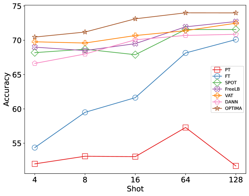
Figure 3: Average test performance on MRPC across 16 runs. PT and FT are trained on MRPC directly. The rest use the soft prompt pretrained under the QQP$\rightarrow$MRPC setting as initialization. OPTIMA exhibits the best performance across different few-shot settings.

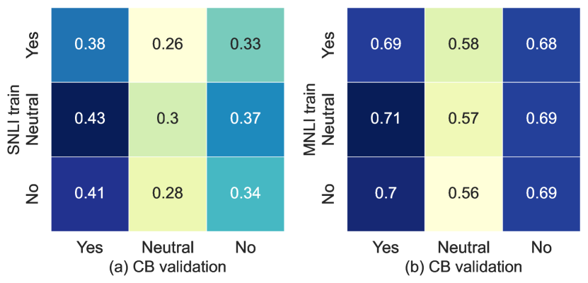
Figure 4: TF-IDF similarity for SNLI, MNLI, and CB, where we treat all text in one class as a document.

3.5 Zero-shot Performance

Zero-shot performance on the target domain is also an effective way to evaluate the learned representations. We show the zero-shot performance in Table 4 and make the following observations.

First, OPTIMA still takes the highest spot in performance in all target domains, outperforming the second best baseline by up to 4.1%. In the source domain, OPTIMA is comparable with the baselines. Second, the ablation baseline, VAT, is consistently surpassed by OPTIMA, which again confirms the utility of our proposal. Third, the state-of-the-art method, SPOT, in the majority of cases produces results with higher variance than the three perturbation-based methods. This suggests that adversarial perturbation is effective against overfitting. Lastly, except in the MNLI $\rightarrow$ SICK task, DANN performs rather poorly across the benchmarks, indicating that DANN is not suitable for prompt tuning.

3.6 Class Similarity and Transfer Learning

We investigate the relationship between domain similarity and transfer learning performance. Due to space constraints, we present the results on CB as the target domain and leave more content to the Appendix. CB is a difficult target. On SNLI, all models in Table 4 achieve in-domain test accuracy greater than $88\%$, but zero-shot SNLI-to-CB transfer obtains accuracy of around $47\%$. This is disappointing given that even Frozen PLM achieves $55.4\%$ on CB.

To investigate the underlying cause, we plot the TF-IDF textual similarities between different domains in Figure 4. We compare SPOT, which performs direct transfer without any smoothness regularization, and OPTIMA in the form of confusion matrices in Figure 5 and F1 scores in Figure 6.

Figure 4(a) shows irregular similarities between classes of SNLI and CB, which explains the difficulty in transfer learning. For example, the SNLI Neutral class is more similar to the CB Yes class than the CB Neural class. The CB Neutral class has low similarity to all SNLI classes. This leads to significant confusion for the few-shot SPOT classifier in the SNLI-to-CB transfer and especially low accuracy for the CB Neutral class (Figure 6). The situation is similar for the MNLI-to-CB transfer. Interestingly, the regularization of OPTIMA is able to alleviate the domain shift and obtain accuracy improvements for the CB No and Neutral classes.

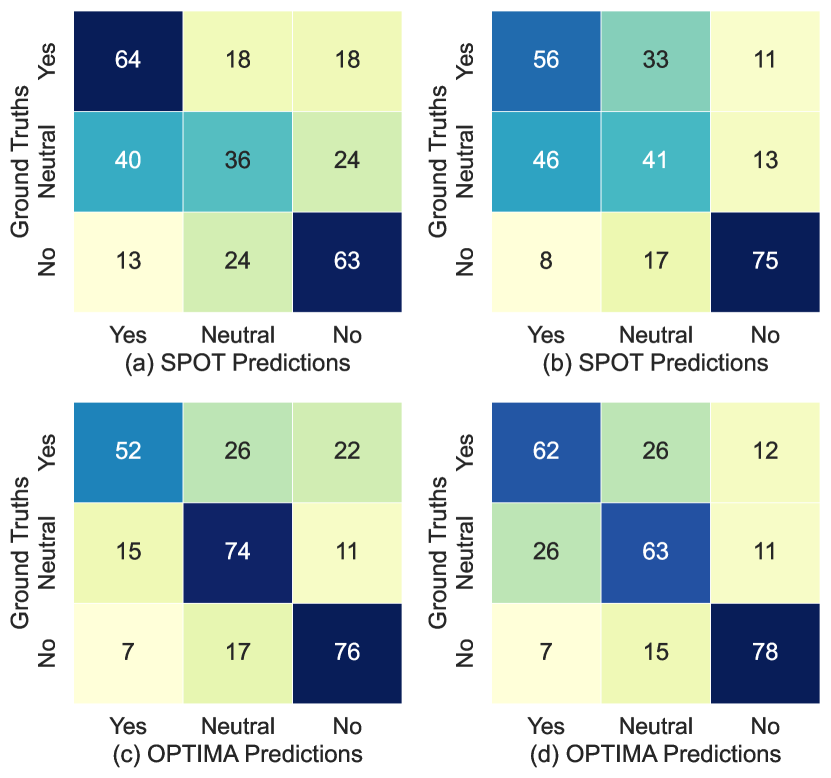
Figure 5: Confusion matrices for 8-shot transfer learning to CB. Each result is the average test accuracy across 16 runs. (a) and (c) refer to SNLI$\rightarrow$CB while (b) and (d) refer to MNLI$\rightarrow$CB setting respectively

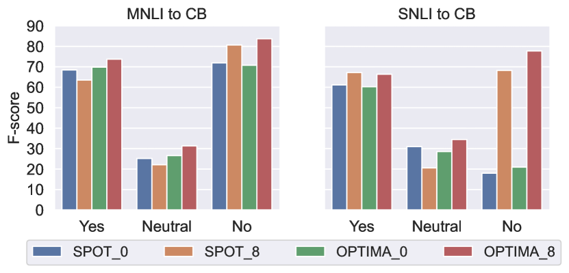
Figure 6: Class-level F1-score on the CB datasets. $\textrm{SPOT}\_0$ and $\textrm{OPTIMA}\_0$ denote zero-shot performance. $\textrm{SPOT}\_8$ and $\textrm{OPTIMA}\_8$ denote 8-shot performance.

4 Related Work

Few-shot Learning with PLMs. Traditional approach for few-shot learning is fine-tuning, where a PLM and a task-specific head are tuned together for the tasks at hand (Zhang et al., 2021; Chen et al., 2020; Das et al., 2022). However, fine-tuning causes high memory consumption as the scale of PLMs increases. To better exploit large frozen PLMs, prompt-based methods have demonstrated excellent few-shot performance on a range of datasets by wrapping test examples in cloze question format for GPT-3 to make predictions (Brown et al., 2020). Prompts are also shown to boost fine-tuning in LM-BFF (Gao et al., 2021), PET (Schick and Schütze, 2021a, b), and PERFECT (Rabeeh et al., 2022).

Transfer Learning for Prompt Tuning. Soft prompt tuning methods (Lester et al., 2021; Li and Liang, 2021; Liu et al., 2022; Hambardzumyan et al., 2021) learn prompts from data and achieve comparable performance with full-model tuning when the PLMs are large enough. SPOT (Vu et al., 2022) proposes to pretrain soft prompts on a set of source-domain datasets and then use the trained soft prompts to boost prompt tuning for target domains. PPT (Gu et al., 2022) introduces unsupervised tasks such as next sentence prediction as the pre-text task for prompt pretraining. After that, the soft prompts are finetuned on the few-shot target-domain data. Wang et al. (2021) pretrain soft prompts across few-shot datasets. Different from these methods, we explore the use of unlabeled target domain data in few-shot prompt tuning.

Consistency Training for NLP. Consistency training methods (Laine and Aila, 2017; Sajjadi et al., 2016; Wei and Zou, 2019; Ng et al., 2020; Xie et al., 2020) force the model to make consistent predictions against small perturbations. For example, Park et al. (2022) produce discrete virtual adversarial noise to the token embeddings. Yoon et al. (2021) apply mixup to perturb the spans of the input texts for text classification. Kim et al. (2021) propose a consistency training framework to enhance the conversational dependency of question answering. Different from these single-domain settings, we consider a cross-domain setting and exploit domain adaptation for regularization.

Neural Domain Adaptation for NLP. Neural domain adaptation Ben-David et al. (2010) includes supervised domain adaptation (SDA) Zhou et al. (2019) and unsupervised domain adaptation (UDA) Wang et al. (2019); Long et al. (2022), depending on whether the target-domain data are labeled or unlabeled. Domain adaptation has been used in various applications such as sentiment analysis Glorot et al. (2011); Dai et al. (2020); Ghosal et al. (2020), machine translation Chu et al. (2017), reading comprehension Wang et al. (2019), and others Shah et al. (2018); Naik and Rose (2020). For a complete survey of UDA in NLP, we refer readers to Ramponi and Plank (2020). In this paper, we do not induce domain-invariant soft prompts but encourage the learned adversarial perturbations to fill in the domain gap and focus on smoothing the decision boundary where source-domain and target-domain data are similar.

5 Conclusions

In this paper, we propose OPTIMA to enhance soft prompt transfer performance by regularizing the training on source domain under perturbations generated with domain adaptation. We extensively evaluate the proposed method. Compared to competitive baselines, soft prompt trained with OPTIMA generalizes better to the source domain and significantly boosts zero-shot and few-shot learning in the target domain. We observe that pre-training soft prompts on a similar dataset confers more benefits than pre-training on a disimilar dataset. We expect the current work to contribute to the wide deployment of PLMs.

Limitations

We identify a few limitations of the current work.

• The domain adaptation problem formulation requires unlabeled data from the target domain. Although unlabeled data are easy to obtain in most cases, doing so might be difficult for some data-scarce domains.

• The proposed regularization technique addresses the situation where the source and target domains have different data distributions. When the two distributions are exactly the same, the technique degenerates to simply adversarial training. When the two distributions are extremely dissimilar, the transfer is unlikely to yield performance improvements. A unified framework that automatically detects domain distances and applies the correct method may be desirable.

• The power of perturbations has the most effect in the few-shot / zero-shot settings. When the target domain has abundant labeled data, the gap between soft prompt tuning and our method will likely diminish.

Appendix A Appendix

A.1 Few-shot Evaluation Protocol

In PET (Schick and Schütze, 2021b), authors evaluated its few-shot performance using a fixed training set. In LM-BFF (Gao et al., 2021), authors conducted more studies on the configuration of few-shot settings and proposed to average 5 randomly sampled few-shot sets. We determine the sample size, 16, based on an statistical analysis on the sample size required for investigating an unknown population mean under student $t$-test. Here we adopt a significance level $\alpha=0.05$, the risk of rejecting a true hypothesis that the performance of one method is better than the other.

For all the cross-domain few-shot learning methods, the few-shot test performance of 3 differently pre-trained soft prompts are averaged for each given $\mathcal{D}_{train}$ and $\mathcal{D}_{dev}$ splits, and we obtain 16 averaged few-shot performance. Then we compute the mean and standard deviation for the 16 test results.

Training Settings. Following (Lester et al., 2021), we use Adafactor (Shazeer and Stern, 2018) as the optimizer and set the learning rate to $0.3$ for all the pre-training tasks on the entire source domain dataset. We use the cosine learning rate scheduler for all methods. For the pre-training stage, we set the maximum number of training steps to $30,000$ and evaluate the models on the validation set every $1,000$ steps. We set the batch size to $8$ for MRPC and QQP, and $18$ for the NLI datasets. For the few-shot learning setting, we set the maximum number of training steps to $1,000$ and evaluate models on $|\mathcal{D}_{dev}|$ every $4$ steps. we set batch size to $4$ for MRPC and QQP, and $6$ for the NLI datasets. All the training are done on NVIDIA V-100 with 32 GB.

	Hybrid Template
T1	$\bm{P}$ $<S_{1}>$ and $<S_{2}>$ are equivalent? [MASK]
T2	$\bm{P}$ hypothesis: $<S_{1}>$ premise: $<S_{2}>$ answer: [MASK]

Table 5: The hybrid templates where $\bm{P}$ represents learnable soft prompts. $<S_{1}>$ and $<S_{2}>$ are sentence pairs. [MASK] represents the labels to be predicted. T1 is the template adopted by the paraphrase detection and question pair classification tasks. T2 is the template adopted by four natural language inference tasks.

Methods	4-shot	8-shot	16-shot	64-shot	128-shot
PT	51.9 $\pm$ 8	53.1 $\pm$ 11	53.0 $\pm$ 9	57.2 $\pm$ 9	51.7 $\pm$ 10
FT	54.4 $\pm$ 12	59.5 $\pm$ 8	61.6 $\pm$ 6	68.2 $\pm$ 4	70.1 $\pm$ 5
SPOT	68.2 $\pm$ 4	68.7 $\pm$ 3	67.9 $\pm$ 5	71.6 $\pm$ 4	71.6 $\pm$ 4
FreeLB	69 $\pm$ 4	68.5 $\pm$ 2	69.5 $\pm$ 2.5	71.9 $\pm$ 1.7	72.7 $\pm$ 1.8
VAT	69.8 $\pm$ 2.7	69.6 $\pm$ 1.9	70.7 $\pm$ 2.7	71.4 $\pm$ 3.1	72.5 $\pm$ 2.9
DANN	66.6 $\pm$ 6.2	63.6 $\pm$ 4.8	70.1 $\pm$ 3.8	70.7 $\pm$ 3.8	70.9 $\pm$ 2.2
OPTIMA	70.5 $\pm$ 3.4	71.2 $\pm$ 1.7	73.1 $\pm$ 2.1	74 $\pm$ 2.7	74 $\pm$ 2.1

Table 6: Average test performance on MRPC dataset, where transfer learning methods are transferred from the QQP dataset.

		SNLI			MNLI
		Yes	Neutral	No	Yes	Neutral	No
CB	Yes	83.7	7.61	8.7	70.43	20.87	8.7
	Neutral	65	20	15	56	44	0
	No	62.5	12.5	25	19.29	20	60.71

Table 7: Confusion matrix for zero-shot performance of SPOT on each class of CB. Results are in $\%$. The bold means the most predicted labels for each of the classes of CB

		SNLI			MNLI
		Yes	Neutral	No	Yes	Neutral	No
CB	Yes	76.52	18.26	6.52	71.3	20	8.7
	Neutral	60	40	0	52	48	0
	No	52.86	29.29	17.86	17.86	20.71	61.43

Table 8: Confusion matrix for zero-shot performance of OPTIMA on each class of CB.

		SNLI			MNLI
		Yes	Neutral	No	Yes	Neutral	No
CB	Yes	63.86	17.93	18.21	56.25	32.61	11.14
	Neutral	40	36.25	23.75	46.25	41.25	12.5
	No	12.95	23.88	63.17	8.04	16.52	75.45

Table 9: Confusion matrix for few-shot performance of SPOT on each class of CB.

		SNLI			MNLI
		Yes	Neutral	No	Yes	Neutral	No
CB	Yes	52.45	25.54	22.01	61.68	26.09	12.23
	Neutral	15	73.75	11.25	26.25	62.5	11.25
	No	7.37	16.96	75.67	6.69	14.96	78.35

Table 10: Confusion matrix for few-shot performance of OPTIMA on each class of CB.

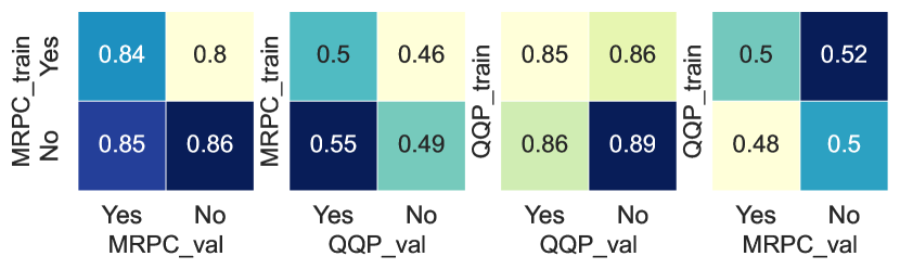
Figure 7: Document similarity for MRPC and QQP datasets between their classes.

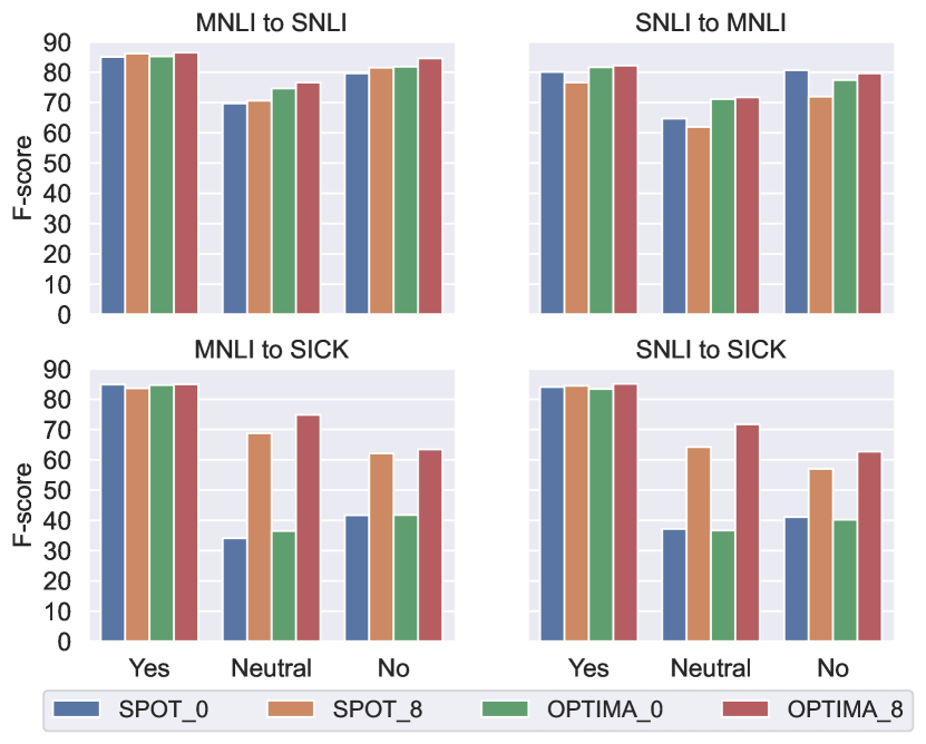
Figure 8: F-score on three classes for NLI datasets. $\textrm{SPOT}\_0$ and $\textrm{OPTIMA}\_0$ are compared for their zero-shot performance. $\textrm{SPOT}\_8$ and $\textrm{OPTIMA}\_8$ are compared for their 8-shot performance.

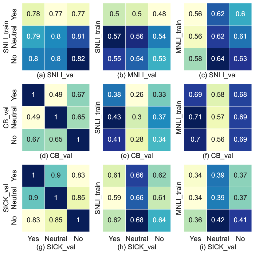
Figure 9: Document similarity using TF-IDF for each pair of NLI datasets.

References

- Ben-David et al. (2010) Shai Ben-David, John Blitzer, Koby Crammer, Alex Kulesza, Fernando Pereira, and Jennifer Wortman Vaughan. 2010. A theory of learning from different domains. Machine learning, 79(1):151–175.
- Bowman et al. (2015) Samuel R. Bowman, Gabor Angeli, Christopher Potts, and Christopher D. Manning. 2015. A large annotated corpus for learning natural language inference. In Proceedings of the 2015 Conference on Empirical Methods in Natural Language Processing, pages 632–642, Lisbon, Portugal. Association for Computational Linguistics.
- Brown et al. (2020) Tom Brown, Benjamin Mann, Nick Ryder, Melanie Subbiah, Jared D Kaplan, Prafulla Dhariwal, Arvind Neelakantan, Pranav Shyam, Girish Sastry, Amanda Askell, et al. 2020. Language models are few-shot learners. Advances in neural information processing systems, 33:1877–1901.
- Chen et al. (2020) Zhiyu Chen, Harini Eavani, Wenhu Chen, Yinyin Liu, and William Yang Wang. 2020. Few-shot NLG with pre-trained language model. In Proceedings of the 58th Annual Meeting of the Association for Computational Linguistics, pages 183–190, Online. Association for Computational Linguistics.
- Chu et al. (2017) Chenhui Chu, Raj Dabre, and Sadao Kurohashi. 2017. An empirical comparison of domain adaptation methods for neural machine translation. In Proceedings of the 55th Annual Meeting of the Association for Computational Linguistics (Volume 2: Short Papers), pages 385–391.
- Cicek and Soatto (2019) Safa Cicek and Stefano Soatto. 2019. Input and weight space smoothing for semi-supervised learning. In Proceedings of the IEEE/CVF International Conference on Computer Vision (ICCV) Workshops.
- Dai et al. (2020) Yong Dai, Jian Liu, Xiancong Ren, and Zenglin Xu. 2020. Adversarial training based multi-source unsupervised domain adaptation for sentiment analysis. In Proceedings of the AAAI Conference on Artificial Intelligence, volume 34, pages 7618–7625.
- Das et al. (2022) Sarkar Snigdha Sarathi Das, Arzoo Katiyar, Rebecca Passonneau, and Rui Zhang. 2022. CONTaiNER: Few-shot named entity recognition via contrastive learning. In Proceedings of the 60th Annual Meeting of the Association for Computational Linguistics (Volume 1: Long Papers), pages 6338–6353, Dublin, Ireland. Association for Computational Linguistics.
- De Marneffe et al. (2019) Marie-Catherine De Marneffe, Mandy Simons, and Judith Tonhauser. 2019. The commitmentbank: Investigating projection in naturally occurring discourse.
- Devlin et al. (2019) Jacob Devlin, Ming-Wei Chang, Kenton Lee, and Kristina Toutanova. 2019. BERT: Pre-training of deep bidirectional transformers for language understanding. In Proceedings of the 2019 Conference of the North American Chapter of the Association for Computational Linguistics: Human Language Technologies, Volume 1 (Long and Short Papers), pages 4171–4186, Minneapolis, Minnesota. Association for Computational Linguistics.
- Elad et al. (2022) Ben Zaken Elad, Goldberg Yoav, and Ravfogel Shauli. 2022. BitFit: Simple parameter-efficient fine-tuning for transformer-based masked language-models. In Proceedings of the 60th Annual Meeting of the Association for Computational Linguistics (Volume 2: Short Papers), pages 1–9, Dublin, Ireland. Association for Computational Linguistics.
- Ganin et al. (2016) Yaroslav Ganin, Evgeniya Ustinova, Hana Ajakan, Pascal Germain, Hugo Larochelle, François Laviolette, Mario Marchand, and Victor Lempitsky. 2016. Domain-adversarial training of neural networks. J. Mach. Learn. Res., 17(1):2096–2030.
- Gao et al. (2021) Tianyu Gao, Adam Fisch, and Danqi Chen. 2021. Making pre-trained language models better few-shot learners. In Proceedings of the 59th Annual Meeting of the Association for Computational Linguistics and the 11th International Joint Conference on Natural Language Processing (Volume 1: Long Papers), pages 3816–3830, Online. Association for Computational Linguistics.
- Ghosal et al. (2020) Deepanway Ghosal, Devamanyu Hazarika, Abhinaba Roy, Navonil Majumder, Rada Mihalcea, and Soujanya Poria. 2020. KinGDOM: Knowledge-Guided DOMain Adaptation for Sentiment Analysis. In Proceedings of the 58th Annual Meeting of the Association for Computational Linguistics, pages 3198–3210, Online. Association for Computational Linguistics.
- Glorot et al. (2011) Xavier Glorot, Antoine Bordes, and Yoshua Bengio. 2011. Domain adaptation for large-scale sentiment classification: A deep learning approach. In ICML.
- Gokaslan and Cohen (2019) Aaron Gokaslan and Vanya Cohen. 2019. Openwebtext corpus.
- Gu et al. (2022) Yuxian Gu, Xu Han, Zhiyuan Liu, and Minlie Huang. 2022. PPT: Pre-trained prompt tuning for few-shot learning. In Proceedings of the 60th Annual Meeting of the Association for Computational Linguistics (Volume 1: Long Papers), pages 8410–8423, Dublin, Ireland. Association for Computational Linguistics.
- Guo et al. (2021) Xu Guo, Boyang Li, Han Yu, and Chunyan Miao. 2021. Latent-optimized adversarial neural transfer for sarcasm detection. In Proceedings of the 2021 Conference of the North American Chapter of the Association for Computational Linguistics: Human Language Technologies, pages 5394–5407, Online. Association for Computational Linguistics.
- Hambardzumyan et al. (2021) Karen Hambardzumyan, Hrant Khachatrian, and Jonathan May. 2021. WARP: Word-level Adversarial ReProgramming. In Proceedings of the 59th Annual Meeting of the Association for Computational Linguistics and the 11th International Joint Conference on Natural Language Processing (Volume 1: Long Papers), pages 4921–4933, Online. Association for Computational Linguistics.
- He et al. (2022) Junxian He, Chunting Zhou, Xuezhe Ma, Taylor Berg-Kirkpatrick, and Graham Neubig. 2022. Towards a unified view of parameter-efficient transfer learning. In International Conference on Learning Representations.
- Houlsby et al. (2019) Neil Houlsby, Andrei Giurgiu, Stanislaw Jastrzebski, Bruna Morrone, Quentin De Laroussilhe, Andrea Gesmundo, Mona Attariyan, and Sylvain Gelly. 2019. Parameter-efficient transfer learning for nlp. In International Conference on Machine Learning, pages 2790–2799. PMLR.
- Hu et al. (2021) Edward J Hu, Yelong Shen, Phillip Wallis, Zeyuan Allen-Zhu, Yuanzhi Li, Shean Wang, Lu Wang, and Weizhu Chen. 2021. Lora: Low-rank adaptation of large language models. arXiv preprint arXiv:2106.09685.
- Huang et al. (2020) W. Ronny Huang, Zeyad Emam, Micah Goldblum, Liam Fowl, Justin K. Terry, Furong Huang, and Tom Goldstein. 2020. Understanding generalization through visualizations. In Proceedings on "I Can’t Believe It’s Not Better!" at NeurIPS Workshops, volume 137 of Proceedings of Machine Learning Research, pages 87–97. PMLR.
- Kim et al. (2019) Dongha Kim, Yongchan Choi, and Yongdai Kim. 2019. Understanding and improving virtual adversarial training. arXiv preprint 1909.06737.
- Kim et al. (2021) Gangwoo Kim, Hyunjae Kim, Jungsoo Park, and Jaewoo Kang. 2021. Learn to resolve conversational dependency: A consistency training framework for conversational question answering. In Proceedings of the 59th Annual Meeting of the Association for Computational Linguistics and the 11th International Joint Conference on Natural Language Processing (Volume 1: Long Papers), pages 6130–6141, Online. Association for Computational Linguistics.
- Kingma and Ba (2015) Diederik P. Kingma and Jimmy Ba. 2015. Adam: A method for stochastic optimization. In ICLR (Poster).
- Laine and Aila (2017) Samuli Laine and Timo Aila. 2017. Temporal ensembling for semi-supervised learning. In ICLR (Poster). OpenReview.net.
- Lester et al. (2021) Brian Lester, Rami Al-Rfou, and Noah Constant. 2021. The power of scale for parameter-efficient prompt tuning. In Proceedings of the 2021 Conference on Empirical Methods in Natural Language Processing, pages 3045–3059, Online and Punta Cana, Dominican Republic. Association for Computational Linguistics.
- Li and Liang (2021) Xiang Lisa Li and Percy Liang. 2021. Prefix-tuning: Optimizing continuous prompts for generation. In Proceedings of the 59th Annual Meeting of the Association for Computational Linguistics and the 11th International Joint Conference on Natural Language Processing (Volume 1: Long Papers), pages 4582–4597, Online. Association for Computational Linguistics.
- Liu et al. (2022) Xiao Liu, Kaixuan Ji, Yicheng Fu, Weng Tam, Zhengxiao Du, Zhilin Yang, and Jie Tang. 2022. P-tuning: Prompt tuning can be comparable to fine-tuning across scales and tasks. In Proceedings of the 60th Annual Meeting of the Association for Computational Linguistics (Volume 2: Short Papers), pages 61–68, Dublin, Ireland. Association for Computational Linguistics.
- Long et al. (2022) Quanyu Long, Tianze Luo, Wenya Wang, and Sinno Pan. 2022. Domain confused contrastive learning for unsupervised domain adaptation. In Proceedings of the 2022 Conference of the North American Chapter of the Association for Computational Linguistics: Human Language Technologies, pages 2982–2995, Seattle, United States. Association for Computational Linguistics.
- Mahabadi et al. (2021) Rabeeh Karimi Mahabadi, James Henderson, and Sebastian Ruder. 2021. Compacter: Efficient low-rank hypercomplex adapter layers. Advances in Neural Information Processing Systems, 34:1022–1035.
- Marelli et al. (2014) Marco Marelli, Stefano Menini, Marco Baroni, Luisa Bentivogli, Raffaella Bernardi, and Roberto Zamparelli. 2014. A SICK cure for the evaluation of compositional distributional semantic models. In Proceedings of the Ninth International Conference on Language Resources and Evaluation (LREC’14), pages 216–223, Reykjavik, Iceland. European Language Resources Association (ELRA).
- Miyato et al. (2016) Takeru Miyato, Andrew M Dai, and Ian Goodfellow. 2016. Adversarial training methods for semi-supervised text classification. In ICLR.
- Miyato et al. (2018) Takeru Miyato, Shin-ichi Maeda, Masanori Koyama, and Shin Ishii. 2018. Virtual adversarial training: a regularization method for supervised and semi-supervised learning. IEEE transactions on pattern analysis and machine intelligence, 41(8):1979–1993.
- Naik and Rose (2020) Aakanksha Naik and Carolyn Rose. 2020. Towards open domain event trigger identification using adversarial domain adaptation. In Proceedings of the 58th Annual Meeting of the Association for Computational Linguistics, pages 7618–7624, Online. Association for Computational Linguistics.
- Ng et al. (2020) Nathan Ng, Kyunghyun Cho, and Marzyeh Ghassemi. 2020. SSMBA: Self-supervised manifold based data augmentation for improving out-of-domain robustness. In Proceedings of the 2020 Conference on Empirical Methods in Natural Language Processing (EMNLP), pages 1268–1283, Online. Association for Computational Linguistics.
- Park et al. (2022) Jungsoo Park, Gyuwan Kim, and Jaewoo Kang. 2022. Consistency training with virtual adversarial discrete perturbation. In Proceedings of the 2022 Annual Conference of the North American Chapter of the Association for Computational Linguistics (Short Papers).
- Rabeeh et al. (2022) Karimi Mahabadi Rabeeh, Zettlemoyer Luke, Henderson James, Mathias Lambert, Saeidi Marzieh, Stoyanov Veselin, and Yazdani Majid. 2022. Prompt-free and efficient few-shot learning with language models. In Proceedings of the 60th Annual Meeting of the Association for Computational Linguistics (Volume 1: Long Papers), pages 3638–3652, Dublin, Ireland. Association for Computational Linguistics.
- Raffel et al. (2020) Colin Raffel, Noam Shazeer, Adam Roberts, Katherine Lee, Sharan Narang, Michael Matena, Yanqi Zhou, Wei Li, and Peter J. Liu. 2020. Exploring the limits of transfer learning with a unified text-to-text transformer. Journal of Machine Learning Research, 21(140):1–67.
- Ramponi and Plank (2020) Alan Ramponi and Barbara Plank. 2020. Neural unsupervised domain adaptation in NLP—A survey. In Proceedings of the 28th International Conference on Computational Linguistics, pages 6838–6855, Barcelona, Spain (Online). International Committee on Computational Linguistics.
- Rücklé et al. (2021) Andreas Rücklé, Gregor Geigle, Max Glockner, Tilman Beck, Jonas Pfeiffer, Nils Reimers, and Iryna Gurevych. 2021. AdapterDrop: On the efficiency of adapters in transformers. In Proceedings of the 2021 Conference on Empirical Methods in Natural Language Processing, pages 7930–7946, Online and Punta Cana, Dominican Republic. Association for Computational Linguistics.
- Sajjadi et al. (2016) Mehdi Sajjadi, Mehran Javanmardi, and Tolga Tasdizen. 2016. Regularization with stochastic transformations and perturbations for deep semi-supervised learning. In Advances in Neural Information Processing Systems, volume 29. Curran Associates, Inc.
- Schick and Schütze (2021a) Timo Schick and Hinrich Schütze. 2021a. Exploiting cloze-questions for few-shot text classification and natural language inference. In Proceedings of the 16th Conference of the European Chapter of the Association for Computational Linguistics: Main Volume, pages 255–269, Online. Association for Computational Linguistics.
- Schick and Schütze (2021b) Timo Schick and Hinrich Schütze. 2021b. It’s not just size that matters: Small language models are also few-shot learners. In Proceedings of the 2021 Conference of the North American Chapter of the Association for Computational Linguistics: Human Language Technologies, pages 2339–2352, Online. Association for Computational Linguistics.
- Shah et al. (2018) Darsh Shah, Tao Lei, Alessandro Moschitti, Salvatore Romeo, and Preslav Nakov. 2018. Adversarial domain adaptation for duplicate question detection. In Proceedings of the 2018 Conference on Empirical Methods in Natural Language Processing, pages 1056–1063, Brussels, Belgium. Association for Computational Linguistics.
- Shazeer and Stern (2018) Noam Shazeer and Mitchell Stern. 2018. Adafactor: Adaptive learning rates with sublinear memory cost. In Proceedings of the 35th International Conference on Machine Learning, volume 80 of Proceedings of Machine Learning Research, pages 4596–4604. PMLR.
- Su et al. (2021) Yusheng Su, Xiaozhi Wang, Yujia Qin, Chi-Min Chan, Yankai Lin, Zhiyuan Liu, Peng Li, Juanzi Li, Lei Hou, Maosong Sun, et al. 2021. On transferability of prompt tuning for natural language understanding. arXiv preprint arXiv:2111.06719.
- Sung et al. (2022) Yi-Lin Sung, Jaemin Cho, and Mohit Bansal. 2022. Lst: Ladder side-tuning for parameter and memory efficient transfer learning. arXiv preprint arXiv:2206.06522.
- Vu et al. (2022) Tu Vu, Brian Lester, Noah Constant, Rami Al-Rfou’, and Daniel Cer. 2022. SPoT: Better frozen model adaptation through soft prompt transfer. In Proceedings of the 60th Annual Meeting of the Association for Computational Linguistics (Volume 1: Long Papers), pages 5039–5059, Dublin, Ireland. Association for Computational Linguistics.
- Wang et al. (2021) Chengyu Wang, Jianing Wang, Minghui Qiu, Jun Huang, and Ming Gao. 2021. TransPrompt: Towards an automatic transferable prompting framework for few-shot text classification. In Proceedings of the 2021 Conference on Empirical Methods in Natural Language Processing, pages 2792–2802, Online and Punta Cana, Dominican Republic. Association for Computational Linguistics.
- Wang et al. (2019) Huazheng Wang, Zhe Gan, Xiaodong Liu, Jingjing Liu, Jianfeng Gao, and Hongning Wang. 2019. Adversarial domain adaptation for machine reading comprehension. In Proceedings of the 2019 Conference on Empirical Methods in Natural Language Processing and the 9th International Joint Conference on Natural Language Processing (EMNLP-IJCNLP), pages 2510–2520, Hong Kong, China. Association for Computational Linguistics.
- Wei and Zou (2019) Jason Wei and Kai Zou. 2019. EDA: Easy data augmentation techniques for boosting performance on text classification tasks. In Proceedings of the 2019 Conference on Empirical Methods in Natural Language Processing and the 9th International Joint Conference on Natural Language Processing (EMNLP-IJCNLP), pages 6382–6388, Hong Kong, China. Association for Computational Linguistics.
- Williams et al. (2018) Adina Williams, Nikita Nangia, and Samuel Bowman. 2018. A broad-coverage challenge corpus for sentence understanding through inference. In Proceedings of the 2018 Conference of the North American Chapter of the Association for Computational Linguistics: Human Language Technologies, Volume 1 (Long Papers), pages 1112–1122. Association for Computational Linguistics.
- Xie et al. (2020) Qizhe Xie, Zihang Dai, Eduard Hovy, Thang Luong, and Quoc Le. 2020. Unsupervised data augmentation for consistency training. Advances in Neural Information Processing Systems, 33:6256–6268.
- Yoon et al. (2021) Soyoung Yoon, Gyuwan Kim, and Kyumin Park. 2021. SSMix: Saliency-based span mixup for text classification. In Findings of the Association for Computational Linguistics: ACL-IJCNLP 2021, pages 3225–3234, Online. Association for Computational Linguistics.
- Zhang et al. (2021) Haode Zhang, Yuwei Zhang, Li-Ming Zhan, Jiaxin Chen, Guangyuan Shi, Xiao-Ming Wu, and Albert Y.S. Lam. 2021. Effectiveness of pre-training for few-shot intent classification. In Findings of the Association for Computational Linguistics: EMNLP 2021, pages 1114–1120, Punta Cana, Dominican Republic. Association for Computational Linguistics.
- Zhou et al. (2019) Joey Tianyi Zhou, Hao Zhang, Di Jin, Hongyuan Zhu, Meng Fang, Rick Siow Mong Goh, and Kenneth Kwok. 2019. Dual adversarial neural transfer for low-resource named entity recognition. In Proceedings of the 57th Annual Meeting of the Association for Computational Linguistics, pages 3461–3471, Florence, Italy. Association for Computational Linguistics.
- Zhu et al. (2020) Chen Zhu, Yu Cheng, Zhe Gan, Siqi Sun, Tom Goldstein, and Jingjing Liu. 2020. Freelb: Enhanced adversarial training for natural language understanding. In International Conference on Learning Representations.