Selfsimilarity relations for torsional oscillations of neutron stars

Abstract

Selfsimilarity relations for torsional oscillation frequencies of neutron star crust are discussed. For any neutron star model, the frequencies of fundamental torsional oscillations (with no nodes of radial wave function, i.e. at $n=0$, and at all possible angular wave numbers $\ell\geq 2$) is determined by a single constant. Frequencies of ordinary torsional oscillations (at any $n>0$ with $\ell\geq 2$) are determined by two constants. These constants are easily calculated through radial integrals over the neutron star crust, giving the simplest method to determine full oscillation spectrum. All constants for a star of fixed mass can be accurately interpolated for stars of various masses (but the same equation of state). In addition, the torsional oscillations can be accurately studied in the flat space-time approximation within the crust. The results can be useful for investigating magneto-elastic oscillations of magnetars which are thought to be observed as quasi-periodic oscillations after flares of soft-gamma repeaters.

1 Introduction

Neutron stars consist of massive cores and thin light envelopes (e.g., Shapiro & Teukolsky, 1983). The core is liquid and contains superdense matter which equation of state (EOS) is still not entirely known. The envelope is only $\sim 1$ km thick and has the mass $\sim 0.01\,\mbox{${\rm M}\odot$}$. It consists of electrons, atomic nuclei, and (at densities $\rho$ higher the neutron drip density $\rho_{\rm drip}\approx 4.3\times 10^{11}$ ${\rm g\leavevmode\nobreak\ cm^{-3}}$) quasi-free neutrons. As a rule, the atomic nuclei constitute Coulomb crystal (e.g. Haensel et al. 2007) which melts only in the very surface layers of the star. The envelope is often called the crust that is divided into the outer ($\rho<\rho_{\rm drip}$) and the inner ($\rho>\rho_{\rm drip}$) crust. The maximum density in the crust ( $\rho_{\rm cc}\sim 1.4\times 10^{14}$ ${\rm g\leavevmode\nobreak\ cm^{-3}}$) is limited by the core.

This paper is devoted to the theory of torsional oscillations of neutron star, in which case only the crystallized shell oscillates, while other layers do not. The star is assumed to be non-magnetic and spherical. Foundation of the theory was laid by Hansen & Cioffi (1980); Schumaker & Thorne (1983) and McDermott et al. (1988). Later developments were numerous (see, e.g., Samuelsson & Andersson 2007; Andersson et al. 2009; Sotani et al. 2012, 2013a, 2013b; Sotani 2016; Sotani et al. 2017b, a, 2018, 2019 and references therein).

The theory started new life after the discovery of quasi-periodic oscillations (QPOs) in spectra of soft-gamma repeaters (SGRs) after giant flares (see Israel et al. 2005; Watts & Strohmayer 2006; Hambaryan et al. 2011; Huppenkothen et al. 2014b, a; Pumpe et al. 2018). SRGs are magnetars possessing superstrong magnetic fields $B\sim 10^{15}$ G (e.g. Olausen & Kaspi 2014; Mereghetti et al. 2015; Kaspi & Beloborodov 2017). Note that seismic activity of SRGs was predicted by Duncan (1998).

Seismology of magnetars has been developed in numerous publications (e.g., Levin 2006, 2007; Glampedakis et al. 2006; Sotani et al. 2007; Cerdá-Durán et al. 2009; Colaiuda et al. 2009; Colaiuda & Kokkotas 2011, 2012; van Hoven & Levin 2011, 2012; Gabler et al. 2011, 2012, 2013b, 2013a, 2016, 2018; Passamonti & Lander 2014; Link & van Eysden 2016; Gabler et al. 2016, 2018). The observed QPO frequencies (after flares of SGR 1806–20, SGR 1900+14 and SGR J1550–5418) fall in the same range (from $\sim 10$ Hz to a few kHz), as the expected frequencies of torsional oscillations of non-magnetic stars. This means that asteroseismology of magnetars can be related to torsional oscillations of non-magnetic stars. In any case the theory of torsional oscillations is basic for testing more complicated seismology of magnetars. Many publications (e.g. Sotani et al. 2007) devoted to the magnetar seismology were mostly focused on standard torsional oscillations.

Nevertheless, the magnetar seiesmology has turned out to be much richer than the theory of non-magnetic stars. It includes magneto-elastic oscillations which can be treated as torsional oscillations in strong magnetic field, but they become coupled to the neutron star core and possibly to the magnetosphere. The magnetic field opens also other types of magnetar oscillations based on propagation of Alfvén waves in the entire star.

Here we turn to pure torsional oscillations and formulate selfsimilarity relations which simplify calculation and analysys of torsional oscillation frequencies. Section 2 outlines the standard theory. Selfsimilarity relations are discussed in Section 3. In Section 4 they are applied to studying torsional oscillation spectrum of neutron stars composed of matter with the BSk21 EOS (as an example). In Section 5 the selfsimilarity relations are applied for analysing torsional oscillation spectra of neutron stars with other EOSs using results of previous work. Section 6 gives a general outlook on interpretation of QPOs, and Section 7 presents conclusions.

2 Torsional oscillations

2.1 Exact formulation of the problem

Theoretical background for studying torsional oscillations of the crust of a non-rotating and non-magnetic neutron star is well known (e.g. Schumaker & Thorne 1983; Sotani et al. 2007). The crustal matter is treated as a poly-crystal (isotropic solid) of the Coulomb lattice of atomic nuclei. The vibrating layer extends from some solidification density just under the stellar surface to the bottom of the crystalline matter at the interface between the crust and liquid stellar core (e.g., Haensel et al. 2007). Here we study linear oscillations in curved space-time neglecting metric perturbations (i.e., in the relativistic Cowling approximation).

The mertic in a spherically symmetric star can be taken in the standard form

$${\rm ds}^{2}=-{\rm e}^{2\Phi}\,{\rm d}t^{2}+{\rm e}^{2\Lambda}\,{\rm d}r^{2}+r^{2}({\rm d}\theta^{2}+\sin^{2}\theta\,{\rm d}\phi^{2}),$$ (1)

where $t$ is Schwarzschild time (for a distant observer), $r$ is a radial coordinate (circumferential radius), $\theta$ and $\phi$ are ordinary spherical angles; $\Lambda$ and $\Phi$ are two metric functions of $r$. At any $r$ one has

$$\exp\Lambda(r)=\frac{1}{\sqrt{1-2Gm(r)/(rc^{2})}},$$ (2)

where $m(r)$ is the gravitational mass enclosed within a sphere of radius $r$, $G$ is the gravitational constant and $c$ is the speed of light.

Let $R$ be the stellar radius, and $M=m(R)$ be the gravitational stellar mass. Outside the star ($r>R$) one has

$$\exp{(\Phi(r))}=\exp(-{\Lambda(r)})=\sqrt{1-r_{\rm g}/r},$$ (3)

where $r_{\rm g}=2GM/c^{2}$ is the Schwarzschild radius.

Torsional oscillations are associated with shear deformations of crystallized matter along spherical surfaces (to avoid energy consuming radial motions of matter elements in strong gravity). In the linear regime, these oscillations are not accompanied by perturbations of density and pressure. Oscillation eigenmodes can be specified by multipolarity $\ell=2,3,\ldots$, azimuthal number $m_{\ell}$ ($-\ell\leq m_{\ell}\leq\ell$), as well as by the number of radial nodes $n=0,1,\ldots$ The eigenfrequencies $\omega=\omega_{\ell n}$ (defined here for a distant observer) are naturally degenerate in $m_{\ell}$ (because the basic stellar configuration is spherical).

In order to find the oscillation spectrum, it is sufficient to set $m_{\ell}=0$. This will be assumed hereafter. Then vibrating matter elements move along circles at fixed $r$ and $\theta$ (only the angle $\phi$ varies). Proper displacements $u_{{\ell n}}^{\phi}$ of matter elements can be written as

$$u_{{\ell n}}^{\phi}=r\,Y_{{\ell n}}(r)\,\exp({\rm i}\omega_{{\ell n}}t)b_{\ell}(\theta),\quad b_{\ell}(\theta)=\,-\frac{\partial}{\partial\theta}P_{\ell}(\cos\theta),$$ (4)

where $P_{\ell}(\cos\theta)$ is a Legendre polynomial.

The dimensionless function $Y_{{\ell n}}(r)$ is the radial part of oscillation amplitude; it is real for our problem. A complex oscillating exponent $\exp({\rm i}\omega_{{\ell n}}t)$ has standard meaning (as a real part); $b_{\ell}(\theta)$ describes the $\theta$-dependence of the oscillation amplitude. For instance, $b_{2}(\theta)=3\cos\theta\,\sin\theta$. At any $\ell$, vibrational motion vanishes along at the ‘vibrational’ axis $z$ [because $b_{\ell}(\theta)\propto\sin\theta$].

The equation for $Y_{{\ell n}}(r)$ reads

$$Y^{\prime\prime}_{{\ell n}}+\left(\frac{4}{r}+\Phi^{\prime}-\Lambda^{\prime}+\frac{\mu^{\prime}}{\mu}\right)Y^{\prime}_{{\ell n}}+\left[\frac{\rho+P/c^{2}}{\mu}\,\omega_{{\ell n}}^{2}{\rm e}^{-2\Phi}\right.$$

$$\left.-\frac{(\ell+2)(\ell-1)}{r^{2}}\right]{\rm e}^{2\Lambda}Y_{{\ell n}}=0.$$ (5)

Here $\rho(r)$ and $P(r)$ are, respectively, the density and pressure of crustal matter, and $\mu(r)$ is the shear modulus.

In order to determine the pulsation frequencies, equatiom (5) has to be solved with the boundary conditions $Y^{\prime}_{{\ell n}}(r_{1})=0$ and $Y^{\prime}_{{\ell n}}(r_{2})=0$ at both (inner and outer) boundaries $r_{1}$ and $r_{2}$ of the crystalline matter. Actually, the type of the boundary condition at $r_{2}$ is unimportant (Kozhberov & Yakovlev, 2020) because torsional oscillations are mostly supported by the inner crust and dragged from there to the outer crust.

Equation (5) was obtained by Schumaker & Thorne (1983) in a more general form, including weak emission of gravitational waves. It reduces to (5) in the relativistic Cowling approximation that is well justified for torsional oscillations.

Note that the quantity

$$v_{\rm s}(r)=\sqrt{\frac{\mu(r)}{\rho+P(r)/c^{2}}},$$ (6)

in the square brackets of equation (5) is a local velocity of the radial shear wave as measured by a local observer. The second term in the square brackets is the contribution of centrifugal forces.

Solving equation (5), one finds $Y_{\ell n}(r)$ and desired eigenfrequencies $\omega_{\ell n}$. The solution is obtained up to some normalization constant. It is convenient to normalize $Y_{{\ell n}}(r)$ by the outer-boundary value $Y_{0}$, that determines angular vibration amplitude of crystallized matter at $r=r_{2}$. The linear regime assumes $Y_{0}\ll 1$.

Equation (5) is basic for exact solution of the formulated linear oscillation problem. It allows one to directly calculate $\omega_{\ell n}$.

2.2 Equivalent exact formulation

Instead of directly solving equation (5), let us use the formal expression for oscillation frequencies

$$\omega_{{\ell n}}^{2}=[B_{{2\ell n}}+(\ell+2)(\ell-1)B_{{1\ell n}}]/A_{{\ell n}},$$ (7)

$$A_{{\ell n}}=\int_{r_{1}}^{r_{2}}{\rm d}r\,r^{4}\,(\rho+P/c^{2})\,{\rm e}^{\Lambda-\Phi}|Y_{{\ell n}}|^{2},$$ (8)

$$B_{2{\ell n}}=\int_{r_{1}}^{r_{2}}{\rm d}r\,\mu r^{4}{\rm e}^{\Phi-\Lambda}|Y^{\prime}_{{\ell n}}|^{2},$$ (9)

$$B_{1{\ell n}}=\int_{r_{1}}^{r_{2}}{\rm d}r\,\mu r^{2}{\rm e}^{\Phi+\Lambda}|Y_{{\ell n}}|^{2}.$$ (10)

It follows from equation (5) (e.g. Schumaker & Thorne 1983; Kozhberov & Yakovlev 2020). It is more complicated but it will be helpful for subsequent analysis in Section 3. It is fully equivalent to directly solving equation (5). This has been checked in numerical results presented below.

In addition to vibration frequencies, one can study vibrational energy $E_{{\ell n}}^{\rm vib}$ in a mode ($\ell,\,n$),

$$E_{{\ell n}}^{\rm vib}=\frac{\mathrm{\pi}\ell(\ell+1)}{2\ell+1}\,\int_{r_{1}}^{r_{2}}{\rm d}r\,\left[\omega_{\ell n}^{2}(\rho+P/c^{2})\,{\rm e}^{\Lambda-\Phi}|Y_{{\ell n}}|^{2}\right.$$

$$\left.+\mu r^{4}{\rm e}^{\Phi-\Lambda}|Y^{\prime}_{{\ell n}}|^{2}+\mu(\ell+2)(\ell-1)r^{2}{\rm e}^{\Phi+\Lambda}|Y_{{\ell n}}|^{2}\right]$$

$$=\frac{2\mathrm{\pi}\ell(\ell+1)}{2\ell+1}A_{{\ell n}}\omega_{\ell n}^{2}.$$ (11)

The first two lines are taken from Schumaker & Thorne (1983) and Kozhberov & Yakovlev (2020); the third line follows from equation (7).

According to equations (7) and (11), the vibration frequencies and energies can be expressed through three integral quantities $A_{{\ell n}}$, $B_{{\ell n}}$ and $B_{{\ell n}}$ given by equations (8)–(10).

Equation (7) can be rewritten as

$$\omega_{{\ell n}}=\sqrt{\widetilde{\omega}_{{\ell n}}^{2}+(\ell+2)(\ell-1)\delta\widetilde{\omega}_{{\ell n}}^{2}},$$ (12)

$$\delta\widetilde{\omega}_{{\ell n}}^{2}=\frac{B_{{1\ell n}}}{A_{{\ell n}}},\quad\widetilde{\omega}_{{\ell n}}^{2}=\frac{B_{2{\ell n}}}{A_{{\ell n}}},$$ (13)

where $\widetilde{\omega}_{{\ell n}}$ and $\delta\widetilde{\omega}_{{\ell n}}$ are two auxiliary frequencies which depend generally on $\ell$ and $n$. In addition to angular frequencies $\omega_{{\ell n}}$, one often needs cyclic frequencies $\nu_{{\ell n}}=\omega_{{\ell n}}/(2\mathrm{\pi})$. A cyclic frequency for a mode $(\ell,n)$ reads

$$\nu_{\ell n}=\left[\widetilde{\nu}_{\ell n}^{2}+(\ell+2)(\ell-1)\,\delta\widetilde{\nu}_{\ell n}^{2}\right]^{1/2}.$$ (14)

3 Oscillation spectrum and its selfsimilarity

3.1 Fundamental and ordinary modes

It is well known that properties of fundamental ($n=0$, no nodes of $Y_{\ell n}(r)$ at $r_{1}<r<r_{2}$) and ordinary ($n>1$, one or more radial nodes) oscillations are very different.

In both cases, the oscillations are mostly formed in the inner crust under the two effects, which are (i) the radial propagation of shear waves with the velocity (6) of $v_{\rm s}\sim 10^{8}$ cm s^-1 and (ii) the meridional propagation with about the same speed due to centrifugal effect. In equation (5) the first and second effects are described, respectively, by the first and second terms in the square brackets. Although all matter elements oscillate only along circles on respective spheres with fixed $r$, vibrational energy and momentum are distributed over entire crystalline shell due to shear nature of elastic deformations.

3.1.1 Fundamental oscillations

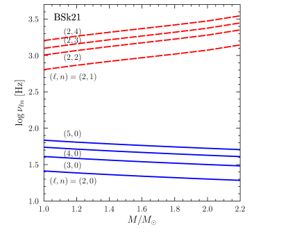
Figure 1: Frequencies $\nu_{\ell n}$ calculated by the exact method of Section 2 for some torsional vibration modes ($\ell,n$) versus mass $M$ of neutron stars with the BSk21 EOS. Four solid (bottom) lines correspond to lowest fundamental modes ($n=0$) with $\ell=$2, 3, 4 and 5. Four dashed upper lines refer to ordinary modes with lowest $\ell=2$ and $n=$1, 2, 3 and 4.

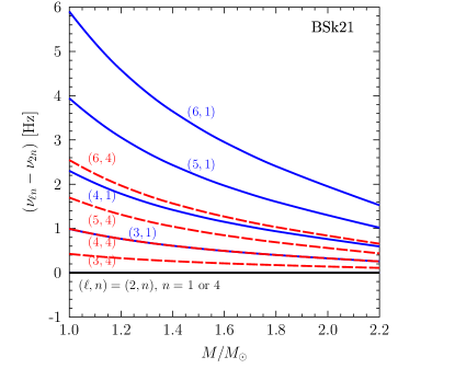
Figure 2: Fine splitting of exactly calculated ordinary vibration frequencies at $n=1$ and $n=4$ (solid and dashed lines, respectively) for neutron stars with the BSk21 EOS as a function of $M$. Splittings of frequencies $\nu_{\ell n}$ are measured from the lowest frequencies $\nu_{21}$ or $\nu_{24}$ in corresponding sequences (from the lowest horizontal line). For both cases, $n=1$ and 4, five fine-structure components are shown (with $\ell$ from 2 to 6).

The fundamental oscillations ($n=0$) are remarkable. Here, the centrifugal effect is most important, and the centrifugal term nearly compensates the shear-wave propagation term in (5) over the inner crust. The shear-momentum transfer in meridional ($\theta$) direction greatly exceeds the transfer in the radial direction so that standing waves are typically formed (e.g. Gabler et al. 2012 ) during propagation of shear perturbations with velocity $v_{\rm s}$ over meridional directions (over typical length-scales $\sim\mathrm{\pi}R$). It takes long time and leads to low oscillation frequencies $\nu\sim 20-100$ Hz. The crystalline crust appears almost non-deformed and only slightly stressed, $Y_{\ell 0}(r)\approx Y_{{\ell 0}}^{{\rm(a)}}=Y_{0}$ being a good first-order approximation (Kozhberov & Yakovlev, 2020). The solutions obtained in this approximation will be labeled with upperscipt (a).

Then equations (7)–(10) yield $B_{2\ell 0}^{(\rm a)}=0$, while $A_{\ell 0}^{(\rm a)}$ and $B_{1\ell 0}^{(\rm a)}$ become independent of $Y_{{\ell 0}}(r)$, being given by simple one 1D integrals which contain well defined functions. Then equation (14) gives $\delta\widetilde{\nu}_{\ell 0}^{\rm(a)}=0$, and the fundamental oscillation frequencies reduce to

$${\nu_{\ell 0}^{\rm(a)}=\nu_{20}^{\rm(a)}\,\sqrt{\frac{(\ell-1)(\ell+2)}{4}},\quad\nu_{20}^{\rm(a)}=\frac{\delta\widetilde{\nu}_{\ell 0}^{\rm(a)}}{2}=\frac{1}{4\mathrm{\pi}}\,\sqrt{\frac{B_{120}^{\rm(a)}}{A_{20}^{\rm(a)}}}.}$$ (15)

Therefore, all fundamental frequencies (for a given neutron star model) are expressed through the lowest frequency $\nu_{20}^{\rm(a)}$. The latter is easily calculated using (8) and (10). The first equation (15) presents selfsimilarity relation for fundamental torsional oscillation. It has been pointed out in a number of publications (e.g., Samuelsson & Andersson 2007; Gabler et al. 2016). Its more strict derivation was given by Kozhberov & Yakovlev (2020).

Fig. 1 shows exactly calculated frequencies (solid lines) of four lowest fundamental torsional oscillation modes ($\ell,n$)=(2,0), (3,0), (4,0) and (5,0). The frequencies are calculated for neutron stars built of matter with the BSk21 equation of state (EOS), as discussed in Section 4. They are plotted versus neutron star mass $M$. The approximately calculated frequencies (15) turn out to be virtually exact, being equal to the exact ones within estimated numerical errors of calculations ($\sim 0.001$ Hz).

3.1.2 Ordinary oscillations and fine splitting

The main differnece of ordinary torsional oscillations ($n>0$) from the fundamental ones is that the centrifugal term in equation (5) is now much smaller than the shear-wave-propagation term. In the first approximation, one can neglect the centrifugal term, which is equivalent to setting $\ell=1$ in (5). This corresponds to purely radial shear wave oscillations. Formally, the case of $\ell=1$ is well known to be forbidden in the adopted relativistic Cowling approximation (it would violate angular momentum conservation). Nevertheless, the solution of (5) at $\ell=1$ does exist, and gives a valid approximate solution for radial wave function of ordinary modes,

$$Y_{\ell n}\approx Y_{\ell n}^{\rm(a)}=Y_{1n}.$$ (16)

This approximation is supported by the results of Kozhberov & Yakovlev (2020). It is clear that the approximate integrals $A_{\ell n}^{\rm(a)}\equiv{\rm A}_{n}$, $B_{2\ell n}^{\rm(a)}\equiv{\rm B}_{2n}$ and $B_{1\ell n}^{\rm(a)}\equiv{\rm B}_{1n}$, calculated from equations (8)–(10), become independent of $\ell$. Accordingly, the auxiliary frequencies $\widetilde{\nu}_{\ell n}^{\rm(a)}\equiv\widetilde{\nu}_{n}$ and $\delta\widetilde{\nu}_{\ell n}^{\rm(a)}\equiv\delta\widetilde{\nu}_{n}$ are also independent of $\ell$, and the approximate oscillation frequencies are given by

$$\nu_{\ell n}^{\rm(a)}=\left[\widetilde{\nu}_{n}^{2}+(\ell+2)(\ell-1)\,\delta\widetilde{\nu}_{n}^{2}\right]^{1/2}.$$ (17)

As a result, a sequence of oscillation frequencies $\nu_{\ell n}$ for a fixed $n$ at different $\ell=2,3,...$ is determined by two easily calculable constants $\widetilde{\nu}_{n}$ and $\delta\widetilde{\nu}_{n}$. The problem of finding the total spectrum $\nu_{\ell n}$ of frequencies for ordinary modes with fixed $n$ reduces to determining one a pair of constants, $\widetilde{\nu}_{n}$ and $\delta\widetilde{\nu}_{n}$. This is another selflimilarity relation valid for ordinary modes, in addition to equation (15) for fundamental modes. Actually, the latter equation can also be dersribed by equation (17) with $\widetilde{\nu}_{0}=0$, so that both equations have the same nature. They reveal universal $\ell$-dependence of oscillation frequencies at any given $n$.

For ordinary modes, in contrast to fundamental ones, the meridional shear momentum transfer is much weaker than the radial one ($\delta\widetilde{\nu}_{n}\ll\widetilde{\nu}_{n}$). Typical pulsation periods are determined by the time of radial shear wave propagation through the inner crust (much shorter than for fundamental modes). Accordingly, the ordinary torsional pulsation frequencies $\nu_{\ell m}\gtrsim 500$ Hz are much higher than for fundamental ones. For example, the dashed curves in Fig. 1 demonstrate exactly calculated frequencies $\nu_{2n}$ at $\ell=2$ and $n=$1, 2, 3 and 4 for stars of different masses with the BSk21 EOS. In logarithmic scale, the dashed curves look nearly equidistant, so that ratios of any pair of frequencies $\nu_{\ell n}$, plotted by dashed lines, are almost independent of $M$. The approximate frequencies turn out to be virtually exact, just as for fundamental modes; see Section 3.1.1.

Formally, the pulsation spectrum is now given by equation (17). In contrast to fundamental modes, $\widetilde{\nu}_{n}$ is not zero, but it is much larger than $\delta\widetilde{\nu}_{n}$. Actually, $\delta\widetilde{\nu}_{n}$ at $n>0$ has the same nature as at $n=0$.

If one fixes $n$ and increases $\ell$, one obtains a sequence of oscillation modes with with slightly higher frequencies. This can be treated as a ‘fine-structure’ splitting of basic frequencies $\nu_{2n}$. The splitting occurs for all frequencies plotted in Fig. 1 by dashed curves. It is too small to be visible in Fig. 1 in logarithmic scale. It is demonstrated in Fig. 2 for the two cases of $n=1$ (solid lines) and $n=4$ (dashed lines). In each case, five fine-structure shifts of components are shown, with $\ell$ varying from 2 to 6. The bottom horizontal line is the basic frequency ($\nu_{21}$ or $\nu_{24}$). Other lines show fine-structure shifts of higher-$\ell$ components. The fine splitting is seen to be really small.

This smallness is a natural consequence of the fact that one typically has $\delta\widetilde{\nu}_{n}\ll\widetilde{\nu}_{n}$ at $n>0$ under physical conditions in neutron star crust. Small ratios $\delta\widetilde{\nu}_{n}/\widetilde{\nu}_{n}\lesssim 0.01$ are associated with the smallness of shear velocity with respect to ordinary sound velocity in the crust ($\mu\ll P$). Note also, that at very large $\ell$ the auxiliary frequencies $\delta\widetilde{\nu}_{n}$ and $\widetilde{\nu}_{n}$ may start to depend on $\ell$ and the validity of the approximate approach may be broken but it may be not very important for applications. The estimates show that it may happen at $\ell\gg 10$.

4 Neutron stars with BSk21 EOS

4.1 Neutron star models

Here, by way of illustration, the theoretical consideration of Section 3 is applied to neutron stars composed of matter with the BSk21 EOS. Various properties of this matter have been accurately approximated by analytic expressions by Potekhin et al. (2013). The EOS is unified – based on the same energy-density functional theory of nuclear interactions in the core and the crust. The liquid core consists of neutrons, protons, electrons and muons, while the crust contains spherical atomic nuclei and electrons, as well as quasi-free neutrons and some admixture of quasi-free protons in the inner crust. For this EOS, the neutron drip density is $\rho_{\rm drip}=4.28\times 10^{11}$ ${\rm g\leavevmode\nobreak\ cm^{-3}}$, and the crust-core interface occurs at $\rho_{\rm cc}=1.34\times 10^{14}$ ${\rm g\leavevmode\nobreak\ cm^{-3}}$.

The EOS is sufficiently stiff, with the maximum neutron star mass $M_{\rm max}=2.27\,\mbox{${\rm M}\odot$}$. The pulsation frequencies $\nu_{\ell n}$ and radial wave functions $Y_{\ell n}(r)$ have been determined by using exact theoretical formulation (Section 2) with the standard boundary conditions, as in Kozhberov & Yakovlev (2020), and with the standard expression for the shear modulus, that was first derived by Ogata & Ichimaru (1990). It has been checked that the approximate frequencies $\nu_{\ell n}^{\rm(a)}$ are virtually exact, as was already pointed out in Section 2. Accordingly, hereafter the upperscript (a) will be mostly dropped. However, one should bear in mind that the virtual exactness may be violated at very large $\ell$; see the end of Section 3.

To be specific, a representative set of models has been chosen with $M/\mbox{${\rm M}\odot$}$=1, 1.2, 1.4,…2.2. In several cases, some models with intermediate $M$ have been considered to check smooth behaviour of the results as a function of $M$.

4.2 Oscillations of the 1.4 ${\rm M}\odot$ star

Table 1: Some torsional oscillation parameters for a $1.4\,\mbox{${\rm M}\odot$}$ neutron star with the BSk21 EOS ($Y_{0}$ is expressed in radians)

$\ell$, $n$	$\nu_{\ell n}$ [Hz]	$E^{\rm vib}_{\ell n}/Y_{0}^{2}$ [erg]
2, 0	23.06	$9.223\times 10^{48}$
2, 1	830.1	$1.899\times 10^{49}$
2, 2	1327.3	$3.348\times 10^{48}$
2, 3	1644.8	$1.990\times 10^{48}$
2, 4	2086.7	$3.898\times 10^{48}$
3, 0	36.45	$3.302\times 10^{48}$
3, 1	830.7	$2.721\times 10^{49}$
3, 2	1327.8	$4.840\times 10^{48}$
3, 3	1645.2	$2.843\times 10^{48}$
3, 4	2086.9	$5.572\times 10^{48}$
4, 0	48.91	$7.729\times 10^{48}$
4, 1	834.5	$3.543\times 10^{49}$
4, 2	1328.5	$6.285\times 10^{48}$
4, 3	1645.7	$3.685\times 10^{48}$
4, 4	2087.3	$7.226\times 10^{48}$

The model with $M=1.4\,\mbox{${\rm M}\odot$}$ has been chosen as basic. In this case the stellar radius is $R=12.60$ km, and the radius of the crust-core interface is $R_{\rm cc}=11.55$ km. The central density of the star is $\rho_{\rm c}=7.30\times 10^{14}$ ${\rm g\leavevmode\nobreak\ cm^{-3}}$.

Table 1 presents 15 torsional oscillation frequencies $\nu_{\ell n}$ of the basic star with $\ell=$ 2, 3 and 4 and $n=$ 0, 1,…4 (including fundamental and ordinary oscillation oscillation modes, particularly, fine splitting). While calculating $\nu_{\ell n}$, the auxiliary frequencies $\widetilde{\nu}_{n}$ and $\delta\widetilde{\nu}_{n}$ have been obtained and their independence of $\ell$ has been checked.

The last column of Table 1 presents vibrational energies $E^{\rm vib}_{\ell n}$ of the same oscillations models computed from equation (11). In the adopted linear approximation, all energies $E^{\rm vib}_{\ell n}$ are proportional to the squared angular vibration amplitude, $Y_{0}^{2}$, of the surface layer. The presented expressions are valid at $Y_{0}\ll 1$ (see Kozhberov & Yakovlev 2020).

4.3 Dependence on neutron star mass

Table 2: Constants $\nu_{02}$, $\widetilde{\nu}_{n}$ and $\delta\widetilde{\nu}_{n}$, which determine all vibration frequencies of fundamental ($\ell,0$) and ordinary ($\ell,n$) torsional vibration modes with $n\leq 4$, for neutron stars with the BSk21 EOS and $M/\mbox{${\rm M}\odot$}=1,\,1.2,\,1.4,\,1.6,\,1.8,\,2$ and 2.2

$M$ (${\rm M}\odot$)	$R$ (km)	$\nu_{20}$ (Hz)	$\widetilde{\nu}_{1}$ (Hz)	$\delta\widetilde{\nu}_{1}$ (Hz)	$\widetilde{\nu}_{2}$ (Hz)	$\delta\widetilde{\nu}_{2}$ (Hz)	$\widetilde{\nu}_{3}$ (Hz)	$\delta\widetilde{\nu}_{3}$ (Hz)	$\widetilde{\nu}_{4}$ (Hz)	$\delta\widetilde{\nu}_{4}$ (Hz)
1.0	12.48	25.87	639.4	14.52	1014	16.56	1255	15.09	1606	15.08
1.2	12.56	24.34	733.5	13.69	1169	15.66	1448	14.49	1844	14.21
1.4	12.60	23.06	829.7	12.98	1327	14.87	1645	13.94	2086	13.47
1.6	12.59	21.94	931.7	12.37	1494	14.17	1855	13.44	2344	12.85
1.8	12.50	20.95	1046	11.83	1680	13.54	2089	12.97	2631	12.28
2.0	12.30	20.05	1184	11.33	1906	12.97	2373	12.53	2980	11.77
2.2	11.81	19.23	1395	10.88	2248	12.44	2803	12.14	3511	11.30

Table 3: Fit parameters $f_{n}$, $\alpha_{n}$, $\beta_{n}$, $\delta f_{n}$, $\delta\alpha_{n}$, and $\delta\beta_{n}$ in equations (19) and (18) for neutron stars with the BSk21 EOS

$n$	$\delta f_{n}$ [Hz]	$\delta\alpha_{n}$	$\delta\beta_{n}$	$f_{n}$ [Hz]	$\alpha_{n}$	$\beta_{n}$
0	44.59	2.411	$-$1.968	0	–	–
1	24.61	2.166	–1.801	1171.7	$-$1.508	1.326
2	27.35	1.750	–1.340	1821.5	$-$1.342	1.163
3	22.04	0.2639	–0.2714	2245	$-$1.316	1.166
4	25.60	2.198	–1.843	2936	$-$1.488	1.306

At the next step the consideration of Section 4.2 is extended to neutron stars of different masses. To this aim, the frequencies of the same 15 vibration modes as in Table 1 have been computed for seven values of $M/\mbox{${\rm M}\odot$}=$1, 1.2,…,2.2. For any $M$, the auxiliary frequencies $\delta\widetilde{\nu}_{n}$ and $\widetilde{\nu}_{n}$ have also been found at $n\leq 4$. These results are presented in Table 2 and plotted in Figs. 3 and 4. The second column of Table 2 lists the radii $R$ of neutron star models.

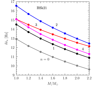
Figure 3: Auxiliary frequencies $\delta\widetilde{\nu}_{n}$ in equation (14) for neutron stars (with the BSk21 EOS) of different masses at $n=$0, 1,…4. Filled dots show the calculated values (Table 2); lines are analytic approximations (equation (18)).

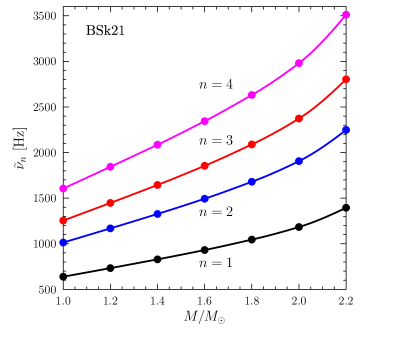
Figure 4: The same as in Fig. 3 but for the auxiliary frequencies $\widetilde{\nu}_{n}$ at $n=$ 1,…4 (with $\widetilde{\nu}_{0}=0$). Lines show analytic approximations (19).

Table 4: Fit parameters $a_{n}$, $c_{n}$ and $\delta c_{n}$, in equation (20) for neutron stars with the BSk21 EOS

$n$	$a_{n}$	$c_{n}$	$\delta c_{n}$
0	0.924	–2.339	2.110
1	0.0133	–2.531	2.307
2	0.000844	$-$2.680	2.418
3	0.000620	$-$1.162	0.933
4	0.000623	$-$1.762	1.635

To simplify using these results, all auxiliary frequencies have been fitted by analytic functions of neutron star mass and radius,

$$\delta\widetilde{\nu}_{n}=\frac{\sqrt{1-\mbox{$x_{\rm g}$}}\,\delta f_{n}}{R_{10}\sqrt{1+\delta\alpha_{n}\mbox{$x_{\rm g}$}+\delta\beta_{n}x_{\rm g}^{2}}},$$ (18)

$$\widetilde{\nu}_{n}=\frac{M_{1}}{R_{10}^{2}}f_{n}\sqrt{1+\alpha_{n}\mbox{$x_{\rm g}$}+\beta_{n}x_{\rm g}^{2}},$$ (19)

where $\mbox{$x_{\rm g}$}\sim 0.3$ is the neutron star compactness parameter that is defined here as $\mbox{$x_{\rm g}$}=r_{\rm g}/R={2GM/(Rc^{2})}$; $R_{10}=R/10$ km, $M_{1}=M/\mbox{${\rm M}\odot$}$; $f_{n}$, $\alpha_{n}$ and $\beta_{n}$ are fit parameters for $\widetilde{\nu}_{n}$; $\delta f_{n}$, $\delta\alpha_{n}$ and $\delta\beta_{n}$ are those for $\delta\widetilde{\nu}_{n}$.

The structure of these fits reflects the nature of slow and faster wave propagations in fundamental and ordinary torsional oscillations (Section 3.1). A characteristic time-scale of the slow meridional heat transport is $\delta\tau\sim v_{\rm s*}R/\sqrt{1-\mbox{$x_{\rm g}$}}$, where $v_{\rm s*}$ is a typical shear velocity (6) in the inner crust, and $1/\sqrt{1-\mbox{$x_{\rm g}$}}$ is the correction factor for a distant observer. Accordingly, equation (18) contains the factor $1/\delta\tau\propto 1/R$. Analogously, characteristic faster radial propagation time scale (with typical shear-sound velocity $v_{\rm s*}$) is $\tau\sim v_{\rm s*}\Delta R$, where $\Delta R$ is a proper depth of the inner crust. The latter can be estimated from the equation of local hydrostatic equilibrium, $\Delta R\sim P_{*}/(g_{\rm s}\rho_{*})$, where $P_{*}$ and $\rho_{*}$ are typical pressure and density in the inner crust and $g_{\rm s}=GM/(R^{2}\sqrt{1-\mbox{$x_{\rm g}$}})$ is the surface gravitational acceleration. As a result, the proper scaling factor in equation (19) is $M/R^{2}$ (the factor $\sqrt{1-\mbox{$x_{\rm g}$}}$ cancels out while transforming to the reference frame of a distant observer). Note that scaling relations similar to (18) and (19) (although less refined) have been discussed in many publications (e.g. Samuelsson & Andersson 2007; Gabler et al. 2012).

Naturally, introducing the above scaling factors in (18) and (19) is not enough to ensure high fit accuracy. One needs some additional tuning. It is done by inserting extra square-root factors containing correcting fit parameters $\alpha_{n}$, $\beta_{n}$, $\delta\alpha_{n}$ and $\delta\beta_{n}$. After that the auxiliary frequencies from Table 2 have been fitted by equations (18) and (19). The resulting fit parameters are listed in Table 3. These fits are very accurate, with maximum relative deviations of the fitted $\widetilde{\nu}_{n}$ and $\delta\widetilde{\nu}_{n}$ values from those in Table 2 smaller than 0.003.

The fits (18) and (19), combined with Table 3, allow one to calculate torsional pulsation frequencies with $n\leq 4$ at any $\ell$ and at $M/\mbox{${\rm M}\odot$}$ from 1 to 2.2. It seems to be the most compact representation of torsional oscillation frequencies $\nu_{\ell n}$.

Now one can introduce relative deviations $\delta_{\ell n}=|\nu_{\ell n}^{\rm fit}/\nu_{\ell n}^{\rm calc}-1|$ of the fitted frequencies from the calculated ones. The root-mean-square (rms) deviation over all 105 frequencies is $\delta_{\rm rms}\approx 0.0021$, and the maximum deviation $\delta_{\rm max}\approx 0.008$ occurs at $\ell=4$, $n=1$ and $M=1\mbox{${\rm M}\odot$}$. For the problem of study, such a fit accuracy seems too good. Although the fit is done for seven values of $M$, it has been checked that it remains equally accurate for intermediate values.

It would be no problem to extend the results for $n>4$. One often assumes [e.g. equation (21) in Samuelsson & Andersson 2007] that with increasing $n$ the frequency $\nu_{\ell n}\approx\widetilde{\nu}_{2n}$ scales proportionally to $n$. This assumption is based on analogy with 1D oscillations in a uniform slab. It is approximately confirmed by calculations of $\nu_{2n}$ at $n=$ 2, 3 and 4 by Sotani et al. (2007) for neutron stars with several EOSs and masses (see their table 4 and Section 5 below). However, this scaling is not the law of nature and can be violated, as seen from Fig.  4. As for the auxiliary frequency $\delta\widetilde{\nu}_{n}$, it is rather small and unimportant in the total frequency $\nu_{\ell n}$. It is expected that replacing $\delta\widetilde{\nu}_{n}$ by $\delta\widetilde{\nu}_{4}$ at $n>4$ would be a reasonable approximation for calculating $\nu_{\ell n}$.

In addition, the quantity $A_{\ell n}\approx A_{n}^{\rm(a)}$ given by equation (8) has been calculated. Here we again use the uppersript (a) to distinguish between approvimate and exact quantites. $A_{n}^{\rm(a)}$ is needed to determine the approximate vibrational energy $E^{\rm vib(a)}_{\ell n}$ from equation (11). Calculations have been done at $n\leq 4$ for the same seven values of $M$. The results are fitted by the expression

$${A_{n}^{\rm(a)}}=10^{42}\,\frac{Y_{0}^{2}R_{10}^{6}\,a_{n}}{M_{1}\,(1+c_{n}x_{g}+\delta c_{n}x_{g}^{2})}\;\;\,{\rm g\,cm^{2}},$$ (20)

where $a_{n}$, $c_{n}$ and $\delta c_{n}$ are dimensionless fit parameters listed in Table 4. Exact values of $E_{\ell n}^{\rm vib}$ have been computed from equations (8) and (11) for the same 105 oscillation modes ($\ell,n$). The rms relative error of the fits is $\approx 0.01$, while the maximum error $\approx 0.024$ occurs at $\ell=4$, $n=0$ and $M=1.2\,\mbox{${\rm M}\odot$}$.

4.4 Torsion oscillations in flat space-time crust

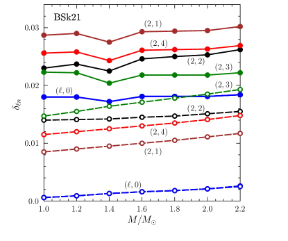
Figure 5: Absolute values of relative deviations $\delta_{\ell n}$ of some vibration frequencies $\nu_{\ell n}^{\rm fs}$, calculated for seven values of $M/\mbox{${\rm M}\odot$}$=1, 1,2,…2.2 in the flat space-time approximation, from those, calculated in full General Relativity. Filled and open dots ( solid and dashed lines) refer, respectively, to $x_{g*}=x_{\rm s}$ and $x_{g*}=x_{\rm cc}$. The vibration modes are ($\ell,n$)= (2,0), (3.0), (4,0), (2,1), (2,2), (2,3) and (2,4). At $n=0$ the deviations $\delta_{\ell n}$ are almost independent of $\ell$ and merge in one solid or dashed curve.

So far all calculations have been done in full General Relativity. Here we check if General Relativity is really needed?

A neutron star crust is usually thin (it thickness is $\sim 1$ km) and contains about $\sim 1$ per cent of the stellar mass. Naturally, the metric (1) in the crust is expected to be close to the Schwarzschild metric, with the metric functions $\Lambda(r)$ and $\Phi(r)$ close to those given by equation (3).

Let us try even simpler approach, with constant $\Lambda$ and $\Phi$ throughout the crust,

$$\Lambda=-\Phi=-{\textstyle\frac{1}{2}}\ln(1-x_{\rm g*}),$$ (21)

where $x_{\rm g*}=2Gm(r_{*})/(c^{2}r_{*})$, and $r_{\rm g*}$ is some fiducial radial coordinate $r=r_{*}$ in the crust. This makes the space-time (1) in the crust artificially flat (although different from the asymptotically flat space-time of a distant observer).

We have solved equation (5) in this approximation for neutron stars with the BSk21 EOS at the same 7 values of $M/\mbox{${\rm M}\odot$}$ from 1 to 2.2, as in Section 4.3, and found flat-space (fs) vibration frequencies $\nu_{\ell n}^{\rm fs}$ for the same values of $\ell$ and $n$ as in Table 1 at several values of $r_{*}$. For all 105 oscillation modes at any $r_{*}$ we have tried, relative deviations $\delta_{\ell n}=|\nu_{\ell n}^{\rm fs}/\nu_{\ell n}-1|$ of $\nu_{\ell n}^{\rm fs}$ from exact frequencies $\nu_{\ell n}$ (determined in full General Relativity) do not exceed a few per cent.

The results for two cases of (I) $r_{*}=R$, $x_{\rm g*}=x_{\rm s}$ ($x_{\rm g*}$ is the same as at the surface) and (II) $r_{*}=R_{\rm cc}$, $x_{\rm g*}=x_{\rm cc}$ (at the crust-core interface) are plotted in Fig. 5. Filled and open dots refer to cases I and II, respectively. In case I the rms deviation is $\approx 0.024$, and the maximum deviation is $\approx 0.03$. In case II one has $\delta_{\rm rms}\approx 0.013$ and $\delta_{\rm max}\approx 0.02$.

If one does not need a very high accuracy, the flat space-time approximation with any $r_{*}$ from $R_{\rm cc}$ to $R$ is reasonably good. Higher accuracy at $r_{*}=R_{\rm cc}$ (case I) is quite understandable – torsional oscillations are mainly formed in the inner crust. Naturally, the Newtonian approximation is accurate because torsional oscillations are fully confined in a thin and light crust. For oscillations of other types which penetrate the neutron star core, the agreement is much worse (as can be easily deduced from the results of Yoshida & Lee 2002).

5 Previous work

5.1 Different EOSs

Table 5: Quantities $\nu_{20}$, $\widetilde{\nu}_{1}$ and $\delta\widetilde{\nu}_{1}$ which determine all vibration frequencies of fundamental ($0,\ell$) and ordinary ($1,\ell$) torsional vibrations of neutron stars with the EOSs, masses and radia considered by Sotani et al. (2007); see the text for details

EoS	$M$	$R$	$\nu_{20}$	$\widetilde{\nu}_{1}$	$\delta\widetilde{\nu}_{1}$
	(${\rm M}\odot$)	(km)	(Hz)	(Hz)	(Hz)
A+DH	1.4	9.49	28.50	1206	15.42
A+DH	1.6	8.95	27.20	1531	14.80
WFF3+DH	1.4	10.82	26.33	941.9	14.36
WFF3+DH	1.6	10.61	25.23	1101	13.76
WFF3+DH	1.8	10.03	24.29	1367	13.17
APR+DH	1.4	12.10	24.60	760.8	13.37
APR+DH	1.6	12.09	23.38	859.8	12.71
APR+DH	1.8	12.03	22.28	965.2	12.17
APR+DH	2.0	11.91	21.27	1083	11.56
APR+DH	2.2	11.65	20.18	1238	11.00
L+DH	1.4	14.66	21.55	529.7	11.68
L+DH	1.6	14.78	20.58	586.0	11.15
L+DH	1.8	14.83	19.67	647.7	10.71
L+DH	2.0	14.82	18.93	712.2	10.26
L+DH	2.2	14.73	18.19	787.9	9.866
L+DH	2.4	14.54	17.54	874.0	9.564
L+DH	2.6	14.13	16.96	995.0	9.173
A+NV	1.4	9.48	28.71	950.5	15.58
A+NV	1.6	8.94	27.38	1190	14.91
WFF3+NV	1.4	10.82	26.69	740.2	14.46
WFF3+NV	1.6	10.61	25.41	865.4	13.80
WFF3+NV	1.8	10.03	24.38	1069	13.28
APR+NV	1.4	11.93	25.16	615.8	13.59
APR+NV	1.6	11.95	23.81	688.0	12.87
APR+NV	1.8	11.92	22.59	769.0	12.25
APR+NV	2.0	11.82	21.43	858.0	11.63
APR+NV	2.2	11.59	20.32	974.1	11.07
L+NV	1.4	13.58	23.17	483.0	12.46
L+NV	1.6	13.82	21.82	524.0	11.76
L+NV	1.8	14.00	20.68	567.2	11.19
L+NV	2.0	14.09	19.68	614.5	10.68
L+NV	2.2	14.11	18.78	666.8	10.19
L+NV	2.4	14.02	17.96	728.8	9.780
L+NV	2.6	13.68	17.20	823.9	9.361

Since the torsional oscillations have been studied in many publications, it is instructive to analyse previous results using the formalism of Sections 3 and 4.

In particular, an extensive calculation of torsional oscillation frequencies of non-magnetic spherical neutron stars was performed by Sotani et al. (2007). The authors presented detailed tables of oscillation frequencies of stars with different EOSs and masses ($M\geq 1.4\,\mbox{${\rm M}\odot$}$). They considered fundamental modes $\nu_{\ell 0}$ with $\ell$= 2, 3,…10 (their table 2), ordinary modes with one radial node, $\nu_{\ell 1}$, with the same $\ell$ (table 3), and lowest-$\ell$ modes, $\nu_{2n}$, with $n=2$, 3 and 4 (table 4).

Sotani et al. (2007) took four EOSs in the neutron star core and two EOSs in the crust. The EOSs in the core were labeled as A (EOS A suggested by Pandharipande 1971, with $M_{\rm max}\approx 1.65\,\mbox{${\rm M}\odot$}$), WFF3 (Wiringa et al. 1988, $M_{\rm max}\approx 1.8\,\mbox{${\rm M}\odot$}$), APR (Akmal et al. 1998, $M_{\rm max}\approx 2.35\,\mbox{${\rm M}\odot$}$) and L (Pandharipande & Smith 1975, $M_{\rm max}\approx 2.7\,\mbox{${\rm M}\odot$}$). The EOSs in the crust were labeled as DH and NV; they were constructed by Douchin & Haensel (2001) and Negele & Vautherin (1973), respectively. Their use yields almost the same $M_{\rm max}$ for a fixed EOS in the core.

Recent progress allowed one to accurately measure (constrain) masses of heavy neutron stars in binary systems. In particular, Antoniadis et al. (2013) and Fonseca et al. (2021) reported the masses of two millisecond pulsars in compact binaries with white dwarfs ($M=2.01\pm 0.04\,\mbox{${\rm M}\odot$}$ for the PSR J0348+0432, and $M=2.08\pm 0.07\,\mbox{${\rm M}\odot$}$ for the PSR J0740+6620). Romani et al. (2022) measured the mass $M=2.35\pm 0.17\,\sun$ of the millisecond “black widow” pulsar J0952–0607 (in pair with a low-mass companion). All deviations are given at 1$\sigma$ level.

These observations indicate that the A and WFF3 EOSs are outdated ( too soft to support most massive pulsars). However, following Sotani et al. (2007), we include them in our analysis in order to broad the bank of theoretical vibration frequencies.

Table 6: Fit parameters $f_{n}$, $\alpha_{n}$, $\beta_{n}$, $\delta f_{n}$, $\delta\alpha_{n}$, and $\delta\beta_{n}$ at $n=0$ and 1 in equations (19) and (18) for neutron stars with the BSk21 EOS; see the text for details

EOS	$\delta f_{0}$ [Hz]	$\delta\alpha_{0}$	$\delta\beta_{0}$	$\delta f_{1}$ [Hz]	$\delta\alpha_{1}$	$\delta\beta_{1}$	$f_{1}$ [Hz]	$\alpha_{1}$	$\beta_{1}$
BSk21	44.59	2.411	$-$1.968	24.61	2.166	–1.801	1171.7	$-$1.508	1.326
APR+DH	42.43	1.322	$-$0.958	22.36	0.978	–0.6743	919.7	–1.015	0.822
APR+NV	45.60	1.972	$-$1.459	24.68	2.081	–1.719	748.9	–1.218	0.997
L+DH	43.89	1.781	$-$1.477	22.90	1.262	–0.890	925.3	–1.066	0.887
L+NV	45.50	1.922	$-$1.380	23.63	1.531	–1.170	748.7	–1.213	0.978

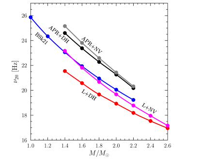
Figure 6: Lowest fundamental oscillation frequency for neutron stars as a function of $M$. The stars are composed of different EOSs: BSk21, APR+NV, APR+DH, L+NV and L+DH. See the text for details.

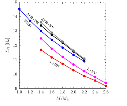
Figure 7: The auxiliary oscillation frequency $\delta\widetilde{\nu}_{1}$ for the same conditions as in Fig. 6.

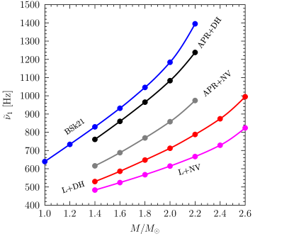
Figure 8: The auxiliary oscillation frequency $\widetilde{\nu}_{1}$ for the same conditions as in Figs. 6 and 7.

Table 5 lists the models used by Sotani et al. (2007). The first three columns give EOS (core+crust), mass and radius of these neutron star models. Column 4 gives the lowest fundamental frequency $\nu_{20}$; it is obtained by fitting the values of $\nu_{\ell 0}$ ($2\leq\ell\leq 10$) from table 2 of Sotani et al. (2007) by equation (15). The fits turn out to be excellent for all models, confirming the validity of (15). Typical fit errors are about $\sim 0.001$. These fits allowed us to find a typo in table 2 for the L+DH EOS at $M=1.4\,\mbox{${\rm M}\odot$}$ and $\ell=5$. One should have $\nu_{50}$=57.0 instead of 60.0.

Columns 5 and 6 present the auxiliary frequencies $\widetilde{\nu}_{1}$ and $\delta\widetilde{\nu}_{1}$ obtained by fitting the frequencies $\nu_{\ell 1}$ at $2\leq\ell\leq 10$ for $n=1$ (table 3 of Sotani et al. 2007) with equation (17)). Again, the fits are fairly accurate, confirming the validity of (17) at $n=1$.

Unfortunately, we cannot extract detailed information on $\widetilde{\nu}_{n}$ and $\delta\widetilde{\nu}_{n}$ with $n\geq 2$ from the data of Sotani et al. (2007) (except for the approximate scaling $\nu_{n}\propto{n}$ mentioned in Section 4.3). Nevertheless, we can check the dependence of $\nu_{20}$, $\widetilde{\nu}_{1}$ and $\delta\widetilde{\nu}_{1}$ (collected in Table 5) on neutron star mass using the scaling equations (18) and (19) (as in Section 4 for the BSk21 EOS). Again, taking models with different masses but one EOS, the scaling relations turn out to be very accurate. For the four EOSs (APR+NV, APR+DH, L+NV, and L+DH) the fit parameters are presented in Table 6 (supplemented by the data for the BSk21 EOS from Table 3). The dependence of $\nu_{20}$, $\delta\widetilde{\nu}_{1}$ and $\widetilde{\nu}_{1}$ on stellar mass for these five EOSs is plotted, respectively, in Figs 6, 7 and 8. The curves are seen to be similar to those for the BSk21 EOS, confirming the correctness of the general description of torsional vibration modes (Section 3). While fitting the data presented in Table 6, a misprint in table 1 of Sotani et al. (2007) has been found: the radius of the $2\mbox{${\rm M}\odot$}$ neutron star with the L+DH EOS should be equal to $R=14.82$ km.

5.2 Crust bottom as a special place

Let us stress that torsional oscillations of non-magnetic spherical neutron stars, discussed above, have been computed neglecting some effects. These effects occur mainly near the bottom of the inner crust; it is as a special place to control torsional oscillations.

First of all, nuclear physics is uncertain there, mostly due to uncertain density dependence of the nuclear symmetry energy. It affects the fraction of protons in the matter and the shear modulus $\mu$. Secondly, $\mu$ is also affected by the effects of finite temperature (which were first considered by Strohmayer et al. 1991). Thirdly, one should mention superfluidity of quasi-free neutrons in the inner crust, which reduces the enthalpy density $P+\rho c^{2}$ of the matter ( the inertial mass density involved in torsional vibrations). Such effects were studied, for instance, by Sotani et al. (2012, 2013b, 2013a); Sotani et al. (2015); Sotani (2016); Sotani et al. (2016). Note also that $\mu$ can be influenced by plasma screening of Coulomb interaction between atomic nuclei (e.g. Strohmayer et al. 1991, Baiko 2015, Chugunov 2022) and by finite sizes of the nuclei (as analyzed by Sotani et al. 2022 on the level of intuitive estimates and by Zemlyakov & Chugunov 2022 on reliable theoretical basis). The respective changes of oscillation frequencies appear noticeable and contain information on nuclear symmetry energy, superfluidity, neutron star mass, radius and compactness.

All these effects can easily be included in the theoretical description of Sections 3, 4 and 5.1 in a unified manner. Appropriate fitting of oscillation frequencies could be performed; it can be simpler and more natural than the fitting proposed in the cited publications (e.g., in Sotani 2016).

Additional complications can be introduced by a layer of nuclear pasta (e.g. Haensel et al. 2007 and references therein) which contains exotic, highly non-spherical nuclear clusters. It can appear or not appear, depending on assumed nuclear interaction model in the layer between the bottom of the crust of spherical nuclei and the neutron star core. Sotani et al. (2017a, b, 2018, 2019) performed calculations of torsional oscillations in the presence of the nuclear pasta layers. They used the standard model of nuclear pasta as a sequence of spherical shells containing phases of cylindrical nuclear structures, nuclear plates, inverted cylinders, and inverted spheres. The crucial question is if such structures can be described in the approximation of isotropic solid, with some effective shear modulus $\mu(r)$? According to Sotani et al. (2019), the dependence $\mu(r)$ within the nuclear pasta contains strong jumps. They complicate calculating torsional oscillations.

Another problem is that, aside of the standard model of nuclear pasta, there are many other models which do not confirm stratification of different pasta layers but predict mixtures of various phases (e.g., glassy quantum nuclear plasma of Newton et al. 2022). In the absence of well established model of nuclear pasta, its effect on torsional oscillations remains uncertain.

It seems that the uncertainties of many parameters at the crust bottom can bias theoretical interpretation of pure torsional oscillations of non-magnetic stars. They will equally bias magneto-elastic oscillations of magnetars.

6 Bursts, QPOs and their interpretation

It is widely thought that oscillations of neutron stars can be triggered by powerful bursts and superbursts occurring within the stars. The best candidates would be superbursts of neutron stars which enter compact X-ray binaries with low-mass companions. It is known that these neutron stars do not possess strong magnetic fields. Superbursts might generate standard torsional oscillations of non-magnetic crust.

Superbursts (e.g., in’t Zand 2017; Galloway & Keek 2017) are rare events. They are thought to be powered by explosive burning of carbon that is produced during nuclear evolution of accreted matter. Carbon can survive in the crust to densities $\rho\sim(10^{7}-10^{10})$ ${\rm g\leavevmode\nobreak\ cm^{-3}}$ and then explode (e.g. Altamirano et al. 2012; Keek et al. 2012). Unfortunately, no oscillations related to superbursts have been observed so far.

Currently, the main attention is paid to QPOs observed in the afterglow of flares of SGR 1806–20, SGR 1900+14, and SGR J1550–5418 (see, e.g., Israel et al. 2005; Watts & Strohmayer 2006; Hambaryan et al. 2011; Huppenkothen et al. 2014b, a; Mereghetti et al. 2015; Kaspi & Beloborodov 2017; Pumpe et al. 2018). The frequencies of these QPOs fall in the same range (from $\sim 10$ Hz to a few kHz), as the expected frequencies of torsional oscillations of non-magnetic stars. The magnetic fields of SGRs, $B\sim 10^{15}$ G, are sufficiently strong to affect oscillations of these stars.

These QPOs are interpreted in two ways. The first way is to use the theory of torsional oscillations in non-magnetic spherical stars (e.g. Sotani et al. 2007, 2012, 2013a, 2013b; Sotani 2016; Sotani et al. 2017a, b, 2018, 2019). In particular, these interpretations include tuning of frequencies with the effects at the crust bottom (Section 5.2).

Other QPO interpretations are based on the theory of oscillations of magnetized neutron stars (e.g., Levin 2006, 2007; Glampedakis et al. 2006; Sotani et al. 2007; Cerdá-Durán et al. 2009; Colaiuda et al. 2009; Colaiuda & Kokkotas 2011, 2012; van Hoven & Levin 2011, 2012; Gabler et al. 2011, 2012, 2013b, 2013a, 2016, 2018; Passamonti & Lander 2014; Link & van Eysden 2016). A summary of this theory can be found in Gabler et al. (2016, 2018). The theory predicts the existence of magneto-elastic oscillations of the crust. They are torsional oscillations modified by magnetic field. However, in contrast to pure torsional oscillations, the magneto-elastic oscillations are coupled to the core and magnetosphere via Alfvén waves.

In addition, the theory predicts global oscillations of a magnetic star based on Alfvén waves. In particular, they contain the so called lower, upper and edge QPOs. They are mainly localized under the crust and are determined by strength and geometry of open and closed magnetic field lines. These oscillations strongly depend on the physics of stellar core (on EOS, superfluidity/superconductivity, magnetic field strength and geometry). Since these properties are rather uncertain, the predicted QPOs can be different, which complicates unambiguous theoretical interpretation of observations. If the magnetic field at the crust bottom is higher than a few times of $10^{15}$ G, the elastic crust may become of little importance.

It seems that all present interpretations of QPOs face the problem of too wide space of many parameters which are currently rather uncertain. Hopefully, the solutions will converge.

7 Conclusions

Standard exact calculation of torsional oscillation frequencies $\nu_{\ell n}$ for a spherical non-magnetic neutron star, based on equation (5), is outlined in Section 2.1. It is valid for a star with crystalline crust that is treated as isotropic solid described by some shear modulus $\mu(r)$. An equivalent formulation of the same problem is suggested in Section 2.2.

Based on the latter formulation, an approximate method for finding $\nu_{\ell n}$ is developed (Section 3). An oscillation frequency $\nu_{\ell n}$ of any mode with fixed number $n=$0, 1, 2, …of radial modes but different orbital numbers $\ell=$2, 3, …can be presented in the form (17), being determined by two auxiliary frequencies, $\widetilde{\nu}_{n}$ and $\delta\widetilde{\nu}_{n}$, independent of $\ell$. The approximate equation (17) appears virtually exact, at least for not too large $\ell$. It predicts a very simple $\ell$-dependence of $\nu_{\ell n}$ that gives a selfsimilarity relation for a star of fixed mass $M$ and EOS.

For fundamental oscillations ($n=0$, Section 3.1.1), $\widetilde{\nu}_{0}=0$ and the spectrum (15) is determined only by small $\delta\widetilde{\nu}_{0}$ (due to inefficient meridional shear-wave energy-momentum transfer). For ordinary torsional modes ($n>0$, Section 3.1.2), both auxiliary frequencies contribute to $\nu_{\ell n}$, with $\delta\widetilde{\nu}_{n}\ll\widetilde{\nu}_{n}$ (and $\delta\widetilde{\nu}_{n}\sim\delta\widetilde{\nu}_{0}$). Higher auxiliary frequencies $\widetilde{\nu}_{n}$ are associated with more intensive radial shear wave motions.

Section 4 is devoted to neutron stars of different $M$ with the BSk21 EOS, as an example. In particular, simple selfsimililar fit equations (18) and (19) for auxiliary frequencies $\delta\widetilde{\nu}_{n}$ and $\widetilde{\nu}_{n}$ are proposed, as functions of $M$. They appear to be very accurate for the BSk21 EOS. Section 5 demonstrates that they are equally accurate for other EOSs considered previously by Sotani et al. (2007).

One can generate a set of values $\widetilde{\nu}_{n}$ and $\delta\widetilde{\nu}_{n}$ (like in any line of Table 2) for a neutron star of fixed mass $M$ and calculate oscillation frequencies $\nu_{\ell n}$ using equation (17). Moreover, one can take tables of $\widetilde{\nu}_{n}$ and $\delta\widetilde{\nu}_{n}$ (e.g. from Table 2) for a range of $M$ (at a fixed EOS) and interpolate the these values as functions of $M$ using equations (19) and (18). In this way one gets a simple and compact description (like Table 3) of torsional oscillation frequencies for all stars with given EOS and microphysics of dense matter. The same can be done for calculating vibration energies.

Section 4.4 shows that torsional oscillation frequencies can be accurately calculated using the flat space-time approximation. It is expected that this approximation can be accurate in studying magneto-elastic oscillations in the crust of magnetized neutron stars. It would greatly simplify semi-analytic consideration of such oscillations, at least at not too high magnetic fields. This would be useful for a firm search of magneto-elastic oscillations in the spectra of magnetar’s QPOs.

Section 5.2 outlines current uncertainties of microphysical functions ($\rho(r)$, $P(r)$ and $\mu(r)$), which enter the basic equation (5), at the crust bottom. These uncertainties seem significant; much work is required to reduce them.

Finally, Section 6 discusses prospects of applying the obtained results for interpretation of observations.

Data availability

The data underlying this article will be shared on reasonable request to the authors.

References

- Akmal et al. (1998) Akmal A., Pandharipande V. R., Ravenhall D. G., 1998, Phys. Rev. C, 58, 1804
- Altamirano et al. (2012) Altamirano D., et al., 2012, MNRAS, 426, 927
- Andersson et al. (2009) Andersson N., Glampedakis K., Samuelsson L., 2009, MNRAS, 396, 894
- Antoniadis et al. (2013) Antoniadis J., et al., 2013, Science, 340, 448
- Baiko (2015) Baiko D. A., 2015, MNRAS, 451, 3055
- Cerdá-Durán et al. (2009) Cerdá-Durán P., Stergioulas N., Font J. A., 2009, MNRAS, 397, 1607
- Chugunov (2022) Chugunov A. I., 2022, arXiv e-prints, p. arXiv:2207.14649
- Colaiuda & Kokkotas (2011) Colaiuda A., Kokkotas K. D., 2011, MNRAS, 414, 3014
- Colaiuda & Kokkotas (2012) Colaiuda A., Kokkotas K. D., 2012, MNRAS, 423, 811
- Colaiuda et al. (2009) Colaiuda A., Beyer H., Kokkotas K. D., 2009, MNRAS, 396, 1441
- Douchin & Haensel (2001) Douchin F., Haensel P., 2001, Astron. Astrophys., 380, 151
- Duncan (1998) Duncan R. C., 1998, ApJ, 498, L45
- Fonseca et al. (2021) Fonseca E., et al., 2021, ApJ, 915, L12
- Gabler et al. (2011) Gabler M., Cerdá Durán P., Font J. A., Müller E., Stergioulas N., 2011, MNRAS, 410, L37
- Gabler et al. (2012) Gabler M., Cerdá-Durán P., Stergioulas N., Font J. A., Müller E., 2012, MNRAS, 421, 2054
- Gabler et al. (2013a) Gabler M., Cerdá-Durán P., Stergioulas N., Font J. A., Müller E., 2013a, Phys. Rev. Lett., 111, 211102
- Gabler et al. (2013b) Gabler M., Cerdá-Durán P., Font J. A., Müller E., Stergioulas N., 2013b, MNRAS, 430, 1811
- Gabler et al. (2016) Gabler M., Cerdá-Durán P., Stergioulas N., Font J. A., Müller E., 2016, MNRAS, 460, 4242
- Gabler et al. (2018) Gabler M., Cerdá-Durán P., Stergioulas N., Font J. A., Müller E., 2018, MNRAS, 476, 4199
- Galloway & Keek (2017) Galloway D. K., Keek L., 2017, arXiv e-prints
- Glampedakis et al. (2006) Glampedakis K., Samuelsson L., Andersson N., 2006, MNRAS, 371, L74
- Haensel et al. (2007) Haensel P., Potekhin A. Y., Yakovlev D. G., 2007, Neutron Stars. 1. Equation of State and Structure. Springer, New York
- Hambaryan et al. (2011) Hambaryan V., Neuhäuser R., Kokkotas K. D., 2011, A&A, 528, A45
- Hansen & Cioffi (1980) Hansen C. J., Cioffi D. F., 1980, ApJ, 238, 740
- Huppenkothen et al. (2014a) Huppenkothen D., et al., 2014a, ApJ, 787, 128
- Huppenkothen et al. (2014b) Huppenkothen D., Heil L. M., Watts A. L., Göğü\textcommabelows E., 2014b, ApJ, 795, 114
- Israel et al. (2005) Israel G. L., et al., 2005, ApJ, 628, L53
- Kaspi & Beloborodov (2017) Kaspi V. M., Beloborodov A. M., 2017, Annual Rev. Astron. Astrophys., 55, 261
- Keek et al. (2012) Keek L., Heger A., in’t Zand J. J. M., 2012, ApJ, 752, 150
- Kozhberov & Yakovlev (2020) Kozhberov A. A., Yakovlev D. G., 2020, MNRAS, 498, 5149
- Levin (2006) Levin Y., 2006, MNRAS, 368, L35
- Levin (2007) Levin Y., 2007, MNRAS, 377, 159
- Link & van Eysden (2016) Link B., van Eysden C. A., 2016, ApJ, 823, L1
- McDermott et al. (1988) McDermott P. N., van Horn H. M., Hansen C. J., 1988, ApJ, 325, 725
- Mereghetti et al. (2015) Mereghetti S., Pons J. A., Melatos A., 2015, Space Sci. Rev., 191, 315
- Negele & Vautherin (1973) Negele J. W., Vautherin D., 1973, Nuclear Phys. A, 207, 298
- Newton et al. (2022) Newton W. G., Cantu S., Wang S., Stinson A., Kaltenborn M. A., Stone J. R., 2022, Phys. Rev. C, 105, 025806
- Ogata & Ichimaru (1990) Ogata S., Ichimaru S., 1990, Phys. Rev. A, 42, 4867
- Olausen & Kaspi (2014) Olausen S. A., Kaspi V. M., 2014, Astrophys. J. Suppl., 212, 6
- Pandharipande (1971) Pandharipande V. R., 1971, Nuclear Phys. A, 178, 123
- Pandharipande & Smith (1975) Pandharipande V. R., Smith R. A., 1975, Physics Letters B, 59, 15
- Passamonti & Lander (2014) Passamonti A., Lander S. K., 2014, MNRAS, 438, 156
- Potekhin et al. (2013) Potekhin A. Y., Fantina A. F., Chamel N., Pearson J. M., Goriely S., 2013, Astron. Astrophys., 560, A48
- Pumpe et al. (2018) Pumpe D., Gabler M., Steininger T., Enßlin T. A., 2018, A&A, 610, A61
- Romani et al. (2022) Romani R. W., Kandel D., Filippenko A. V., Brink T. G., Zheng W., 2022, ApJ, 934, L18
- Samuelsson & Andersson (2007) Samuelsson L., Andersson N., 2007, MNRAS, 374, 256
- Schumaker & Thorne (1983) Schumaker B. L., Thorne K. S., 1983, MNRAS, 203, 457
- Shapiro & Teukolsky (1983) Shapiro S. L., Teukolsky S. A., 1983, Black holes, white dwarfs, and neutron stars: The physics of compact objects. Wiley-Interscience, New York
- Sotani (2016) Sotani H., 2016, Phys. Rev. D, 93, 044059
- Sotani et al. (2007) Sotani H., Kokkotas K. D., Stergioulas N., 2007, MNRAS, 375, 261
- Sotani et al. (2012) Sotani H., Nakazato K., Iida K., Oyamatsu K., 2012, Phys. Rev. Lett., 108, 201101
- Sotani et al. (2013a) Sotani H., Nakazato K., Iida K., Oyamatsu K., 2013a, MNRAS, 428, L21
- Sotani et al. (2013b) Sotani H., Nakazato K., Iida K., Oyamatsu K., 2013b, MNRAS, 434, 2060
- Sotani et al. (2015) Sotani H., Iida K., Oyamatsu K., 2015, Phys. Rev. C, 91, 015805
- Sotani et al. (2016) Sotani H., Iida K., Oyamatsu K., 2016, New Astron., 43, 80
- Sotani et al. (2017a) Sotani H., Iida K., Oyamatsu K., 2017a, MNRAS, 464, 3101
- Sotani et al. (2017b) Sotani H., Iida K., Oyamatsu K., 2017b, MNRAS, 470, 4397
- Sotani et al. (2018) Sotani H., Iida K., Oyamatsu K., 2018, MNRAS, 479, 4735
- Sotani et al. (2019) Sotani H., Iida K., Oyamatsu K., 2019, MNRAS, 489, 3022
- Sotani et al. (2022) Sotani H., Togashi H., Takano M., 2022, arXiv e-prints, p. arXiv:2209.05416
- Strohmayer et al. (1991) Strohmayer T., Ogata S., Iyetomi H., Ichimaru S., van Horn H. M., 1991, ApJ, 375, 679
- Watts & Strohmayer (2006) Watts A. L., Strohmayer T. E., 2006, ApJ, 637, L117
- Wiringa et al. (1988) Wiringa R. B., Fiks V., Fabrocini A., 1988, Phys. Rev. C, 38, 1010
- Yoshida & Lee (2002) Yoshida S., Lee U., 2002, A&A, 395, 201
- Zemlyakov & Chugunov (2022) Zemlyakov N. A., Chugunov A. I., 2022, arXiv e-prints, p. arXiv:2209.05821
- in’t Zand (2017) in’t Zand J., 2017, in Serino M., Shidatsu M., Iwakiri W., Mihara T., eds, 7 years of MAXI: monitoring X-ray Transients. p. 121
- van Hoven & Levin (2011) van Hoven M., Levin Y., 2011, MNRAS, 410, 1036
- van Hoven & Levin (2012) van Hoven M., Levin Y., 2012, MNRAS, 420, 3035