Evaluation of stationarity regions in measured non-WSSUS 60 GHz mmWave V2V channels

Abstract

Due to high mobility in multipath propagation environments, vehicle-to-vehicle (V2V) channels are generally time and frequency variant. Therefore, the criteria for wide-sense stationarity (WSS) and uncorrelated scattering (US) are just satisfied over very limited intervals in the time and frequency domains, respectively. We test the validity of these criteria in measured vehicular $60$ GHz millimeter wave (mmWave) channels, by estimating the local scattering functions (LSFs) from the measured data. Based on the variation of the LSFs, we define time-frequency stationarity regions, over which the WSSUS assumption is assumed to be fulfilled approximately. We analyze and compare both line-of-sight (LOS) and non-LOS (NLOS) V2V communication conditions.

We observe large stationarity regions for channels with a dominant LOS connection, without relative movement between the transmitting and receiving vehicle.

In the same measured urban driving scenario, modified by eliminating the LOS component in the post-processing, the channel is dominated by specular components reflected from an overpassing vehicle with a relative velocity of $56$ km/h. Here, we observe a stationarity bandwidth of $270$ MHz. Furthermore, the NLOS channel, dominated by a single strong specular component, shows a relatively large average stationarity time of $16$ ms, while the stationarity time for the channel with a rich multipath profile is much shorter, in the order of $5$ ms.

© 2022 IEEE. Personal use of this material is permitted. Permission from IEEE must be obtained for all other uses, in any current or future media, including reprinting/republishing this material for advertising or promotional purposes, creating new collective works, for resale or redistribution to servers or lists, or reuse of any copyrighted component of this work in other works.

I Introduction

Beyond fifth generation (B5G) wireless communication technology is supposed to enhance the current systems by offering new wide-bandwidth communication channels. Furthermore, new technologies are developed to suit ever extending requirements of vehicular wireless communication. As a suitable solution for this task, communication over millimeter wave (mmWave) frequency band is proposed. However, the vehicular channels show challenging characteristics due to high mobility and rapidly changing scattering environment. Moreover, the Doppler spectrum may vary over the time-frequency domain, limiting the validity assumption of wide-sense stationarity (WSS) [1]. Nevertheless, the changing channel environment causes variations in the delay spectrum, violating the uncorrelated scattering (US) criterion. Furthermore, as the carrier frequency increases, the Doppler shift becomes more severe. Hence, the before mentioned stationarity issues are magnified, and we conclude that mmWave vehicle-to-vehicle (V2V) channels are in general non-WSS US.
However, the validity of many channel models and design of wireless transceivers is dependent on WSS US assumption. Therefore, it is important to analyze the size of stationarity regions, as time-frequency area, in which WSS US criteria are approximately satisfied.
A theoretical approach to defining stationarity regions is given in [2]. Further, multiple papers investigate the non-WSS US behavior of the measured channels. The authors in [3] and [4] show spatial variation phenomenon, observing the fading process and defining channel stationarity as a function of a distance from the original position. [4] analyses the effect of having a line-of-sight (LOS) as a contrast to a non-LOS (NLOS) connection, showing that the spatial variation is not as severe in LOS as in the NLOS conditions. Experimental contributions for V2V communication, to the identification of stationarity regions in time and frequency, for $5$ GHz band, are presented in [5]. The authors in [6] analyze the stationarity in the time domain depending on different V2V $5$ GHz measurement scenarios. However, to the best of our knowledge, the stationarity investigation for $60$ GHz band has not been shown yet for vehicular communication.
We analyze the behavior of a real measured V2V $60$ GHz channel for typical LOS urban scenarios. Furthermore, in order to compare the results with a NLOS scenario, we modify the measured channel, by eliminating the LOS component in the post-processing. We define local scattering function (LSF), by using the concepts described in [2], and follow its variation over time and frequency. By calculating collinearity between LSF s, and setting a threshold, we define time and frequency, over which LSF is approximately constant. Hence, we quantify the consecutive time-frequency regions with approximately satisfied WSS US condition, called stationarity regions.
In Section II we introduce a definition of LSF, and discuss its parametrization. The measured V2V mmWave channel scenarios, analyzed in this paper, are described in Section III. In Section IV, we introduce the criteria for defining the channel as stationary. Furthermore, in Section V, we present the evaluation of stationarity regions for the defined scenarios. Conclusions are presented in Section VI.

II Local Scattering Function and Parameterization

The time-varying channels are characterized by the discrete channel transfer function, sampled with $T_{s}$ resolution is time and $f_{s}$ in frequency, written as

$$\boldsymbol{H}[s,q]=H(sT_{s},qf_{s}).$$ (1)

We define $s\in[1,\cdots,S]$ and $q\in[1,\cdots,Q]$, $s$ and $q$ being indices in time and frequency domain. Now, we can express the total measurement bandwidth and recorded time as $B=Qf_{s}$ and $T_{\text{total}}=ST_{s}$. Statistical properties of vehicular channels in general do not remain constant over an arbitrary time nor frequency. Therefore, we define time-frequency regions, consisting of $N$ samples in the time and $M$ in frequency domain, in which the stationarity requirements are satisfied. By sequencing the channel transfer function, given in (1), in the stationarity regions we define the local transfer functions, $\boldsymbol{\hat{H}_{k_{t},k_{f}}}[s^{\prime},q^{\prime}]$. $s^{\prime}\in[1,\cdots,N]$ and $q^{\prime}\in[1,\cdots,M]$ denote local time and frequency indices, and $k_{t}$ and $k_{f}$ the indices of each local region in time and frequency

$$k_{t}\in[1,\cdots,K_{t}],\hskip 5.0ptK_{t}=\lfloor\dfrac{S-N}{\Delta_{t}}\rfloor+1,~{}\text{and}$$ (2a)

$$k_{f}\in[1,\cdots,K_{f}],\hskip 5.0ptK_{f}=\lfloor\dfrac{Q-M}{\Delta_{f}}\rfloor+1.$$ (2b)

$\Delta_{t}$ and $\Delta_{f}$ describe time and frequency shift between each two consecutive local transfer functions, expressed in number of samples. The operator $\lfloor\cdot\rfloor$ rounds the number to the nearest lower integer. We denote $\boldsymbol{\hat{H}_{k_{t},k_{f}}}$ as a matrix form of $k_{t}^{\text{th}},k_{f}^{\text{th}}$ local transfer function, containing $N\times M$ elements of time and frequency samples. We have to consider that by taking larger stationarity region we risk the violation of WSS US assumption, but gain higher LSF delay-Doppler resolution.
In order to decrease the variance, we calculate multiple independent spectral estimates by applying multitaper estimator. Here, we define orthogonal data tapers, with each taper providing good protection against leakage, similarly as given in [5]. For tapering function, we use an index limited sequence, with energy concentrated within the selected bandwidth, known as discrete prolate spheroidal sequence (DPSS). The total number of tapers is given by $IJ$, $I$ being the number of sequences in time and $J$ in frequency. When setting the number of tapers, we have to pay attention to the trade-off between the variance reduction and biasing increase. More precisely, by increasing the number of used tapers the variance decreases but at the cost of biasing enlargement [7]. When we increase the number of tapers, we also have to consider the appropriate energy concentration bandwidth $2W_{t}$, defined as a multiple of fundamental frequency

$$W_{t}=\dfrac{a}{NT_{s}},\hskip 5.0pta>1.$$ (3)

Setting $W_{t}$ higher allows for the larger number of tapers with good leakage properties [7]. In the further text, we will express the bandwidth by providing the value of $NW_{t}=\tfrac{a}{T_{s}}$. Here, we want to emphasize, by using DPSS with index limited maximal energy concentration in time, and band limited in the Doppler domain, increasing $W_{t}$ leads to decrease in the resolution in terms of Doppler. Analogously, we define the DPSS in frequency domain. Furthermore, we define the time-frequency taper function

$$\boldsymbol{G_{w}}[s^{\prime},q^{\prime}]=\boldsymbol{u_{i}}[s^{\prime}]\boldsymbol{\tilde{u}_{j}}[q^{\prime}],\hskip 5.0pts^{\prime}\in[1,\cdots,N],q^{\prime}\in[1,\cdots,M],$$ (4)

with $i\in[1,\cdots,I]$, $j\in[1,\cdots,J]$ and $w=iJ+j$. We write the taper function (4) as a matrix $\boldsymbol{G_{w}}$, of dimension $N\times M$. Now we define the matrix form of windowed channel transfer function

$$\boldsymbol{\hat{\mathcal{H}}^{(G_{w})}_{k_{t},k_{f}}}=\boldsymbol{\hat{H}_{k_{t},k_{f}}}\odot\boldsymbol{G_{w}},$$ (5)

where $\odot$ denotes the element-wise Hadamard product. Applying discrete symplectic Fourier transform (DSFT), we obtain tapered Doppler-variant impulse response

$$\boldsymbol{\hat{S}_{k_{t},k_{f}}^{(G_{w})}}=\boldsymbol{F}_{N}\boldsymbol{\hat{\mathcal{H}}^{(G_{w})}_{k_{t},k_{f}}}\boldsymbol{F}_{M}^{H},$$ (6)

$\boldsymbol{F}_{i}$ and $\boldsymbol{F}_{i}^{H}$ representing discrete Fourier transform (DFT) and inverse DFT (IDFT) matrix of size $i$. By applying $IJ$ orthogonal tapers, we create multiple realizations of the same channel, and we calculate the multitaper estimate of the LSF with uniform weighting across the tapered Doppler-variant impulse responses

$$\boldsymbol{\hat{C}_{k_{t},k_{f}}}=\dfrac{1}{IJ}\sum_{w=1}^{IJ}\boldsymbol{\hat{S}_{k_{t},k_{f}}^{(G_{w})}}.$$ (7)

III Measurement Scenarios

This work deals with the definitions of stationarity regions in measured V2V mmWave channels. The measurement campaign took place in an urban street environment, downtown Vienna, Austria. The channel is obtained at the central frequency $f_{c}=60$ GHz, with a frequency resolution $f_{s}=4.96$ MHz, and the $Q=103$ samples in frequency domain. Furthermore, the time resolution is $T_{s}=129.1$ $\mu$s, and we are dealing with $S=5920$ time snapshots. The detailed description of measurement set-up may be found in [8].
The transmitter and receiver are positioned on the right lane of an urban street, at fixed positions, on a tripod and a car’s rear window, respectively. During the measurement, further vehicles are passing by on the left lane, see Fig. 1. Hence, this scenario resembles an urban overtaking process.
At the transmitter side, a directive horn antenna is employed, directed along the street in driving direction. Hence, it covers the receiver and the overtaking vehicle within the $3$ dB beam width of the antenna. Further, at the receiver, an open-ended waveguide antenna is used, oriented in the driving direction, towards the overtaking vehicle. The measurement starts as the car breaks the first light barrier. The second barrier is placed 3 m after the first one for driving speed estimation. The distance between the transmitting and receiving vehicle is 15 m, leading to about 50 ns time of flight for the LOS channel component.

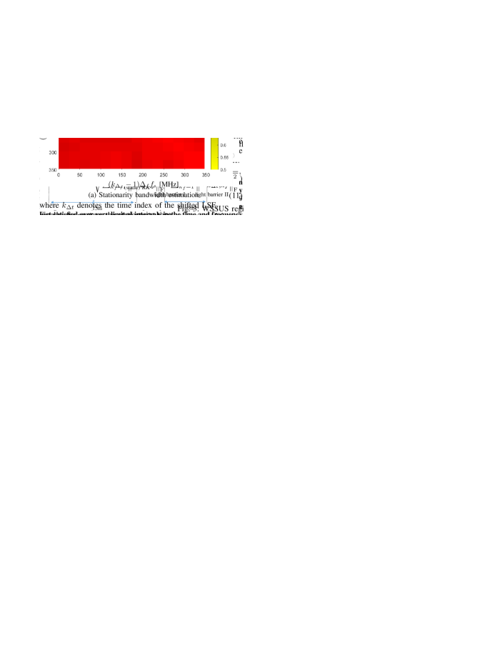
Figure 1: Sketch of the measurement scenario.

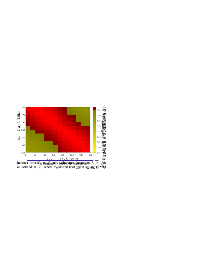
Figure 2: Doppler Power Profile.

In order to better understand the cause of the distribution of stationarity regions, we calculate the Doppler power profile of the given channel, given for each LSF instance as

$$\boldsymbol{\hat{P}_{k_{t},k_{f}}}=\dfrac{1}{M}\boldsymbol{\hat{C}}_{\boldsymbol{k_{t},k_{f}}}\mathbf{1}_{M},$$ (8)

where $\mathbf{1}_{M}$ denotes a column vector of ones, with size $M$. For this investigation, we set channel bandwidth to $B=272.7$ MHz and LSF time shift $\Delta_{t}=5$. Further, we used the LSF size $N=100$, $M=55$, for a potential stationarity time $NT_{s}=$12.9 ms and bandwidth $Mf_{s}=272.7$ MHz, as shown in Fig. 2. Here, we can distinguish between three time periods of the channel characteristics:

• period I - $t=[0,\dots,250]\,$ms: the overtaking vehicle is side-by-side with the receiver vehicle, multiple multipath components (MPCs) appear and cause a large Doppler spread due to the large reflecting surface of the overtaking sport utility vehicle (SUV). Furthermore, as the SUV is moving, the relative speed to the receiver of the different parts of the car differ, causing MPC s with different Doppler shift. Additionally, as the receive antenna is steered along the street, the SUV is outside the main lobe of the antenna’s gain pattern, such that the LOS component is dominant.

• period II - $t=[250,\dots,450]\,$ms: the overtaking vehicle is inside the main lobe of the receive antenna gain pattern, causing a specular component comparable in strength to the LOS. Further, the SUV is oriented with a smaller surface to the receiver, leading to a smaller number of MPC s.

• period III - $t=[450,\dots,760]\,$ms: the vehicle is moving further away, leading to high attenuation of the reflected signal.

In this paper, we evaluate the size of stationarity regions in two scenarios. The first being LOS case, where the direct path from the transmitter to the receiver dominates the channel. Further, we want to obtain a more common urban scenario, where the LOS is blocked, and the wireless communication is performed only through the channel paths reflected of the other vehicles. Here, we describe the overtaking vehicle as a main source of reflecting components, moving with additional 15.8 m/s relative to velocity of transmitter and receiver. We approximate this channel scenario by restricting the measurement data to Doppler shifts $\nu<-258$ Hz, thereby simulating an NLOS scenario.

IV Stationarity Criteria Definition

In section II we describe LSF definition for the channels, where the statistical properties generally cannot be considered WSS in time, nor US in frequency. However, the channel is approximately WSS US within a stationarity region. In order to determine the regions of stationarity, first we calculate the LSF, defined on the assumed local stationary region $T_{LSR}=NT_{s}$ in time and $B_{LSR}=Mf_{s}$ in frequency. Second, we expand this region in time and frequency as long as the LSF stays approximately constant.
As a metric defining whether we may extend the stationarity assumption over the neighboring LSF s, we introduce a spectral distance metric called collinearity, as defined in [9]. We test the enlargement criteria independently in time and in frequency by introducing the collinearity metric for both domains. First, we define the metric to confirm the stationarity in frequency, expressed as

$$\boldsymbol{\gamma^{(f)}}[k_{f},k_{\Delta f}]=\dfrac{\sum_{k_{t}=1}^{K_{t}}\langle\boldsymbol{\hat{C}_{k_{t},k_{f}}},\boldsymbol{\hat{C}_{k_{t},k_{\Delta f}}\rangle}_{\mathrm{F}}}{\sqrt{\sum_{k_{t}=1}^{K_{t}}\left\lVert\boldsymbol{\hat{C}_{k_{t},k_{f}}}\right\rVert^{2}_{\mathrm{F}}\cdot\sum_{k_{t}=1}^{K_{t}}\left\lVert\boldsymbol{\hat{C}_{k_{t},k_{\Delta f}}}\right\rVert^{2}_{\mathrm{F}}}},$$ (9)

where $\langle\mathbf{A},\mathbf{B}\rangle_{\mathrm{F}}=\sum_{i,j}\mathbf{A}[i,j]\mathbf{B}[i,j]$, for $\mathbf{A},\mathbf{B}\in\mathbb{R}^{I\times J}$, denotes Frobenius inner product, and $\lVert\mathbf{A}\rVert_{\mathrm{F}}=\sqrt{\langle\mathbf{A},\mathbf{A}\rangle_{\mathrm{F}}}$ Frobenius norm. Further, $k_{\Delta f}$ is the frequency index of the shifted LSF. As we are calculating the frequency region, over which the LSF is approximately constant, we define a collinearity threshold $\gamma_{th}=0.9$, above which we define the channel as stationary. Hence, we formulate the stationarity bandwidth as,

$$\boldsymbol{f_{stat}}[k_{f}] =(M+(k_{\Delta f}-1)\Delta_{f})f_{s},$$

$$\forall k_{\Delta f}:\boldsymbol{\gamma^{(f)}}[k_{f},k_{\Delta f}]>0.9.$$ (10)

In order to increase the delay resolution of LSF before further examining the validity of the stationarity assumption, we update the size of local transfer function in frequency as $M=\dfrac{\min\limits_{k_{f}}(\boldsymbol{f_{stat}}[k_{f}])}{f_{s}}$. Now we define the collinearity form for the stationarity investigation in the time domain

$$\boldsymbol{\gamma^{(t)}}[k_{t},k_{\Delta t}]=\dfrac{\sum_{k_{f}=1}^{K_{f}}\langle\boldsymbol{\hat{C}_{k_{t},k_{f}}},\boldsymbol{\hat{C}_{k_{\Delta t},k_{f}}\rangle}_{\mathrm{F}}}{\sqrt{\sum_{k_{f}=1}^{K_{f}}\left\lVert\boldsymbol{\hat{C}_{k_{t},k_{f}}}\right\rVert^{2}_{\mathrm{F}}\cdot\sum_{k_{f}=1}^{K_{f}}\left\lVert\boldsymbol{\hat{C}_{k_{\Delta t},k_{f}}}\right\rVert^{2}_{\mathrm{F}}}},$$ (11)

where $k_{\Delta t}$ denotes the time index of the shifted LSF.

Finally, we express the stationarity time

$$\boldsymbol{t_{stat}}[k_{t}] =(N+(k_{\Delta t}-1)\Delta_{t})t_{s},$$

$$\forall k_{\Delta f}:\boldsymbol{\gamma^{(t)}}[k_{t},k_{\Delta t}]>0.9.$$ (12)

V Estimation of stationarity Regions

In this section, we present the estimation of stationarity regions in measured 60 GHz channels. In order to reduce the variance, we apply a multitaper estimator with DPSS tapers as described in section II. We define $IJ=4$, the total number of windows, by using two DPSS tapers in both time and frequency. Further, for bandwidth definition we set $NW_{t}=\tfrac{2}{T_{s}}$ and $MW_{f}=\tfrac{2.5}{f_{s}}$ in time and frequency, respectively. Additionally, to suppress the influence of noise on stationarity estimation, we set a noise threshold 10 dB above the noise level.
A transfer function is approximately constant within the coherence time $T_{c}=\tfrac{1}{\overline{\nu}_{H}}$ and coherence frequency $f_{c}=\tfrac{1}{\overline{\tau}_{H}}$, as defined in [2], where $\overline{\tau}_{H}$ is the root mean square (RMS) delay spread and $\overline{\nu}_{H}$ RMS Doppler spread. Therefore, it gives us a lower bound for the scaling of the local stationarity region. Our measured channel is described by maximum RMS delay spread $\overline{\tau}_{H,\text{max}}=3.75\,$ms and RMS Doppler spread $\overline{\nu}_{H,\text{max}}=250$ Hz [10]. Hence, the minimal coherence time, valid over the whole measurement duration, is $T_{c,\text{min}}=4$ ms, and minimal coherence frequency $f_{c,\text{min}}=266.7$ MHz.
Further, we define a local stationarity region, laying inside the coherence region, spanning over $N=30$, $M=30$ samples in time and frequency, in which we approximate WSS US condition as satisfied. This translates to $3.87$ ms time period and $148.76$ MHz bandwidth. Furthermore, for the time and frequency shift of consecutive LSF regions, we set $\Delta_{t}=5$ and $\Delta_{f}=5$.

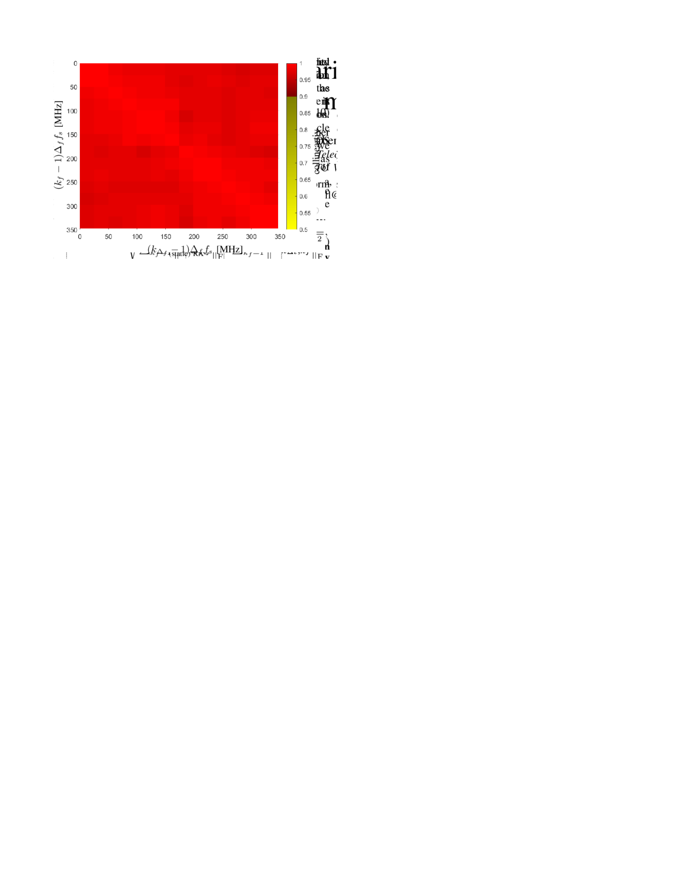
(a) Stationarity bandwidth estimation

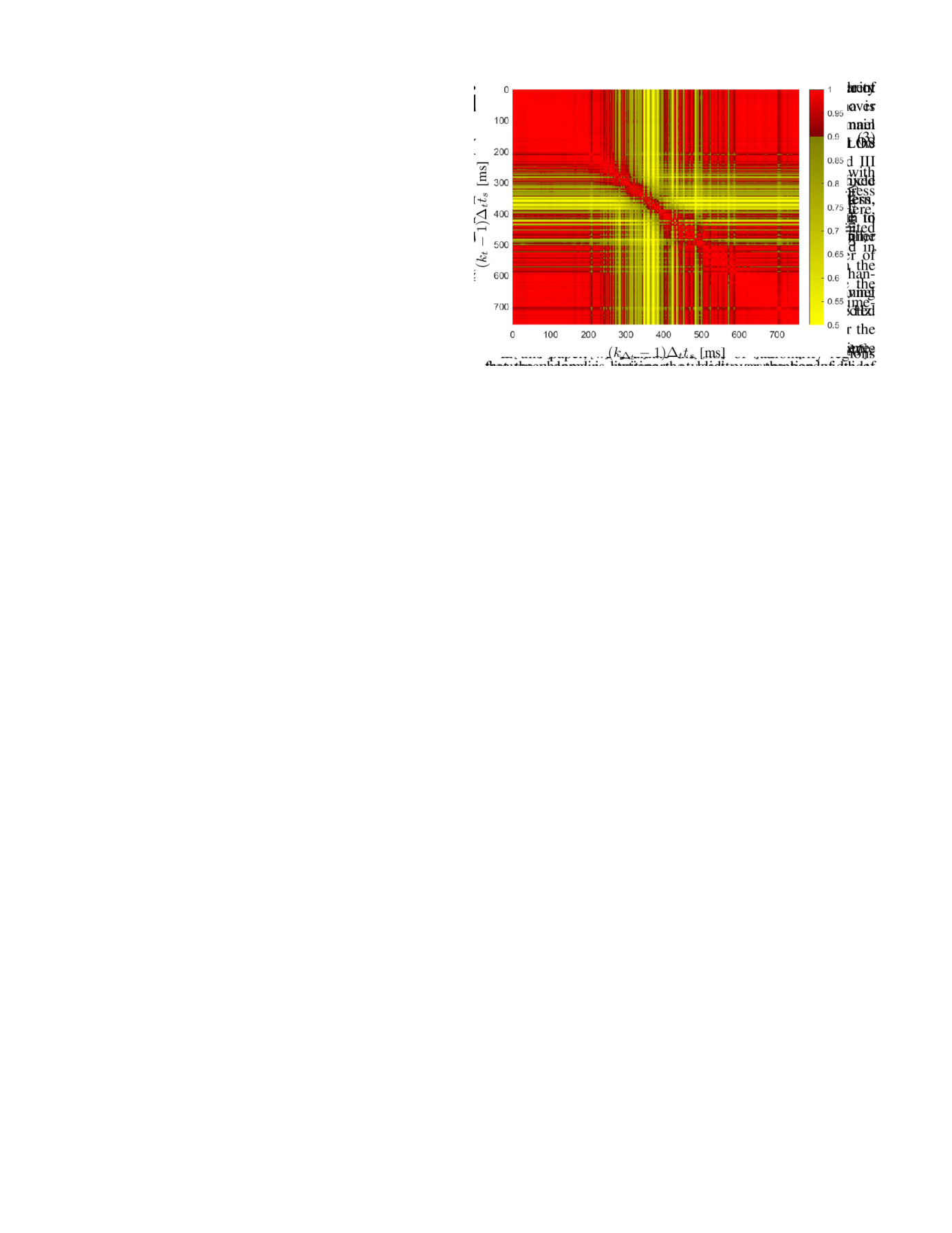
(b) Stationarity time estimation

Figure 3: WSS US regions for LOS scenario.

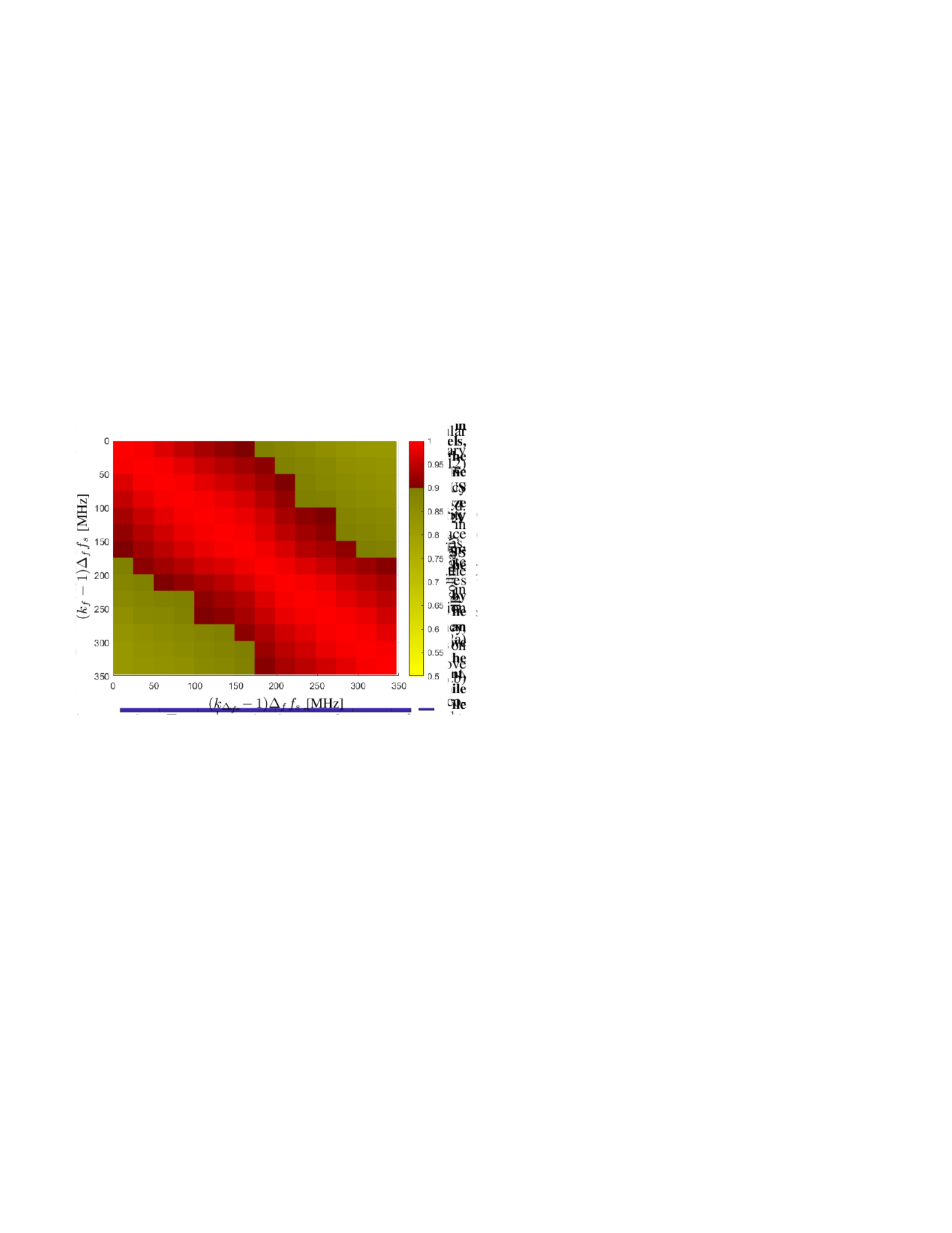
(a) Stationarity bandwidth estimation

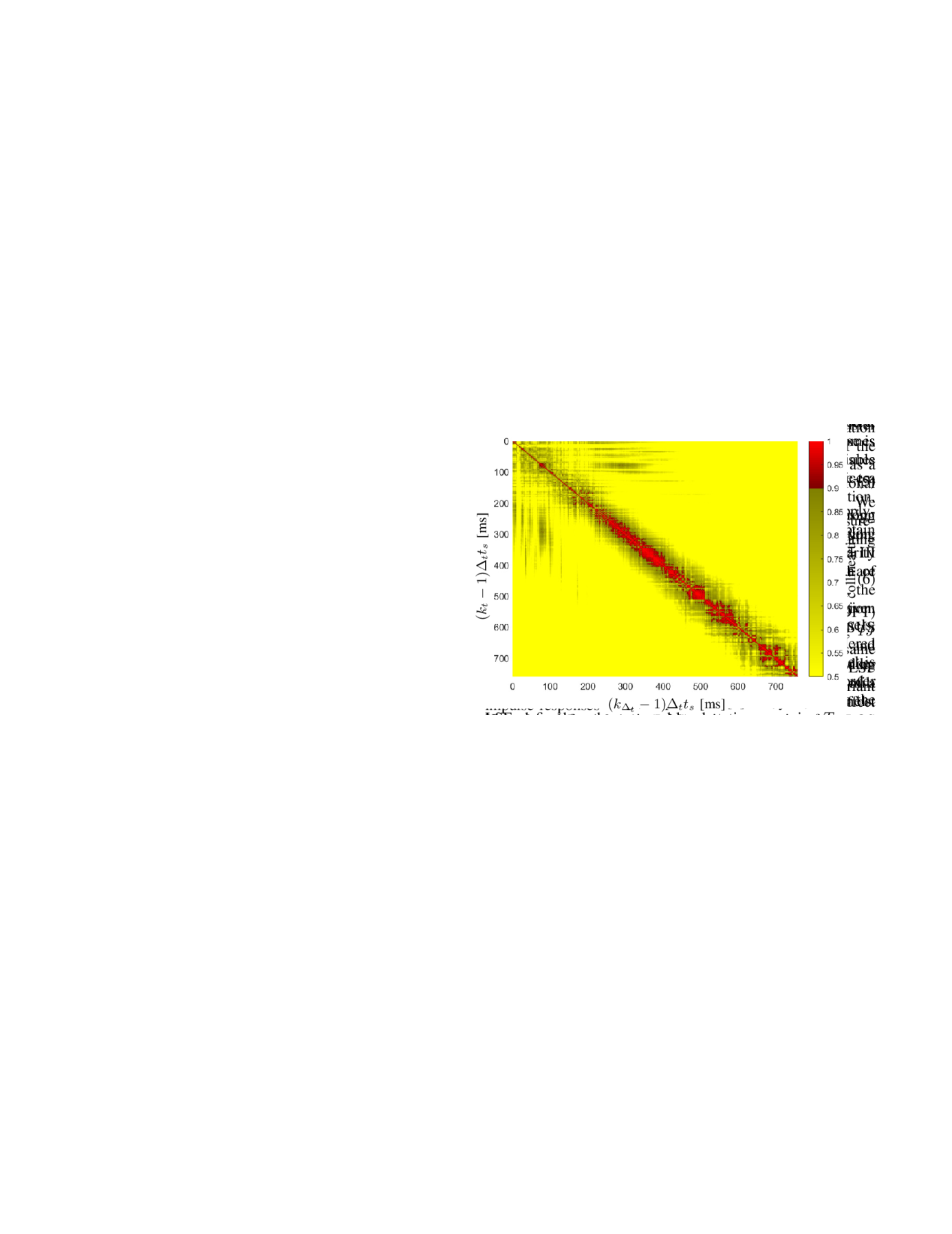
(b) Stationarity time estimation

Figure 4: WSS US regions for NLOS scenario.

First, we investigate, the stationarity characteristics of the channel with a LOS connection. Fig. 3(a) demonstrates the channel stationarity over the whole bandwidth. We can notice that the collinearity values on the diagonal are equal to one, as the LSF is compared with itself. As we move away from the diagonal, the value drops, but never under the defined limit of $0.9$. Therefore, for the investigation of stationarity in time, we increase the local stationarity region to span over the whole bandwidth, $M=103$. Now, we observe the channel stationarity in the time domain, Fig. 3(b). We can notice that the channel is stationary during the whole time period I and III defined in section III, as a LOS connection between the fixed transmitter and receiver dominates the channel. Nevertheless, in the period II when the reflected path is comparable in strength to the LOS, we observe the mean stationarity time of $19.7$ ms.
In order to further investigate the behavior of V2V channels, we obtain the NLOS scenario, observing the channel components characterized by a Doppler shift $\nu<-258$ Hz. Fig. 4(a) shows the values of the collinearity function, over the increasing frequency shift between the two LSF s. We observe that the channel is stationary at least over the bandwidth of $270$ MHz. Furthermore, we enlarge the local stationary region to span over the observed stationary bandwidth, to M=55. Now we analyze the stationarity time, Fig. 4(b). During the period I, the stationarity time is low, in the order of 5 ms. The cause is the channel described by high number of MPC s with variable delay and Doppler shift. Further, in the period II we notice a quasi constant stationary time, with $16$ ms average duration. During this period, the channel is dominated by one strong component, originating from a reflection of a vehicle moving with a constant relative speed of $15.8$ m/s. In the period III the stationarity time is rapidly changing as the strength of the specular channel component decreases and therefore, the residual noise plays higher role in the stationarity estimation.

VI Conclusion

We estimate stationarity regions in measured non-wide-sense stationarity uncorrelated scattering (non-WSS US) millimeter wave (mmWave) vehicle-to-vehicle (V2V) channels. Here, we define a stationarity region, as a time-frequency area, over which the local scattering function (LSF) is approximately constant, and therefore the WSS US assumption is valid approximately. As statistical quantifier, we use collinearity for independent analysis of stationarity in the time and frequency domains.

We conclude that the V2V channels, dominated by a line-of-sight (LOS) connection between two vehicles, which are moving in parallel, exhibit large stationarity regions. Channels with significant specular components originating from an overtaking vehicle moving at urban speed (relative to the others) feature a stationarity time of approximately $20$ ms.

Furthermore, we analyze a case where the LOS is blocked, and specular reflections can be dominant paths, which we consider as non-LOS (NLOS) scenario. The position of an adjacent vehicle relative to two communicating vehicles influences the size and shape of the stationarity region. We observe that in the case of NLOS links with a large number of multipath components (MPCs), the stationarity time becomes very short, in the order of just $5$ ms. In contrast, in cases where the NLOS communication is dominated by one strong specular path, we observe longer stationarity times in the order of $16$ ms. Moreover, in the NLOS V2V scenario, we observe a stationarity bandwidth of $270$ MHz or even larger.

References

- [1] L. Bernadó, T. Zemen, A. Paier, G. Matz, J. Karedal, N. Czink, C. Dumard, F. Tufvesson, M. Hagenauer, A. F. Molisch, and C. F. Mecklenbräuker, “Non-WSSUS vehicular channel characterization at 5.2 GHz-Spectral divergence and time-variant coherence parameters,“ in Proc. 29th URSI General Assembly, Chicago, IL, Aug. 7–16, pp. 198, 2008.
- [2] G. Matz, ”On non-WSSUS wireless fading channels,” in IEEE Transactions on Wireless Communications, vol. 4, no. 5, pp. 2465-2478, Sept. 2005.
- [3] O. Renaudin, V. Kolmonen, P. Vainikainen, and C. Oestges, “Non-stationary narrowband MIMO inter-vehicle channel characterization in the 5-GHz band,” in IEEE Transactions on Vehicular Technology, vol. 59, no. 4, pp. 2007–2015, May 2010.
- [4] Q. Wang et al., ”Spatial Variation Analysis for Measured Indoor Massive MIMO Channels,” in IEEE Access, vol. 5, pp. 20828-20840, 2017.
- [5] L. Bernadó, T. Zemen, F. Tufvesson, A. F. Molisch and C. F. Mecklenbräuker, ”The (in-) validity of the WSSUS assumption in vehicular radio channels,” in Proc. 2012 IEEE 23rd International Symposium on Personal, Indoor and Mobile Radio Communications - (PIMRC), pp. 1757-1762, 2012.
- [6] R. He et al., ”Characterization of Quasi-Stationarity Regions for Vehicle-to-Vehicle Radio Channels,” in IEEE Transactions on Antennas and Propagation, vol. 63, no. 5, pp. 2237-2251, May 2015.
- [7] D. B. Percival, A. T. Walden, Spectral Analysis for Univariate Time Series. Cambridge University Press, 2020.
- [8] E. Zöchmann et al., ”Measured delay and Doppler profiles of overtaking vehicles at 60 GHz,” in Proc. 12th European Conference on Antennas and Propagation (EuCAP 2018), 2018.
- [9] M. Herdin, N. Czink, H. Özcelik and E. Bonek, ”Correlation matrix distance, a meaningful measure for evaluation of non-stationary MIMO channels,” in Proc. 2005 IEEE 61st Vehicular Technology Conference, pp. 136-140 Vol. 1, 2005.
- [10] E. Zöchmann et al., ”Position-Specific Statistics of 60 GHz Vehicular Channels During Overtaking,” in IEEE Access, vol. 7, pp. 14216-14232, 2019.