Distributed Resource Allocation over Multiple Interacting Coalitions: A Game-Theoretic Approach

Abstract

Despite many distributed resource allocation (DRA) algorithms have been reported in literature, it is still unknown how to allocate the resource optimally over multiple interacting coalitions. One major challenge in solving such a problem is that, the relevance of the decision on resource allocation in a coalition to the benefit of others may lead to conflicts of interest among these coalitions. Under this context, a new type of multi-coalition game is formulated in this paper, termed as resource allocation game, where each coalition contains multiple agents that cooperate to maximize the coalition-level benefit while subject to the resource constraint described by a coupled equality. Inspired by techniques such as variable replacement, gradient tracking and leader-following consensus, two new kinds of DRA algorithms are developed respectively for the scenarios where the individual benefit of each agent explicitly depends on the states of itself and some agents in other coalitions, and on the states of all the game participants. It is shown that the proposed algorithms can converge linearly to the Nash equilibrium (NE) of the multi-coalition game while satisfying the resource constraint during the whole NE-seeking process. Finally, the validity of the present allocation algorithms is verified by numerical simulations.

Distributed resource allocation, distributed NE seeking, distributed optimization, multi-agent system, multi-coalition game.

1 Introduction

The past decade has witnessed a significant progress on distributed resource allocation (DRA) over multi-agent networks (MANs), where interacting individual agents cooperate to make the best decision on allocating the group-level resources via information exchange among neighboring agents [1]. The task can be basically modeled as a distributed optimization problem regarding a group-level objective function while subject to the resource constraint described by a coupled equality, and the problem has been extensively studied from various aspects with discrete-time [2, 3, 4, 5, 6, 7, 8] and continuous-time [9, 10, 11, 12, 13, 14] DRA algorithms developed.

Considering the complex interactions of real-world networked systems, the resource allocation problems of multiple coalitions may be coupled with each other. For example, in public finance management, when deciding the allocation of a provincial government’s revenue fund for economic development, the influence of other provinces’ economic development would be taken into account, since cooperation and competition may exist across provinces. In such cases, the DRA problem of multiple coalitions cannot be decoupled into several independent single-coalition DRA problems and solved separately by employing existing DRA algorithms.

Inspired by the above observations, a new model is formulated in this paper for the resource allocation problem of multiple interacting coalitions. In this model, the inputs of each individual agent’s objective function may include the states of agents not only within but also outside the coalition. The group-level objective function of each coalition is the sum of objective functions of all the individual agents therein. In each coalition, the individual agents cooperate to minimize the group-level objective function while subject to the resource constraint described by a coupled equality.

The proposed model can be viewed as a new type of multi-coalition game, as it shares the core feature of capturing the cooperation of agents that belongs to the same coalition and the conflicts of interest among different coalitions. Existing studies on multi-coalition games can be found in [15, 16, 17, 19, 18, 20, 21, 22] and the reference therein, which can be generally classified into two categories according to whether or not intra-coalition consistency constraints are involved. Specifically, the agent states in each coalition are free of coupled constraints in one category of studies [17, 19, 18], while in the other, are demand to reach an agreement [15, 16, 20, 21, 22].

In the seminal work on games of MANs with coalition structure [15], a two-network zero-sum game is formulated, where the agents within each network should agree on a common network state, and the two networks have opposite objective regarding the optimization of a common function of the network states; for this model, distributed Nash equilibrium (NE) seeking algorithms are developed under fixed and switching topologies respectively in [15] and [16]. Then, the work is extended to non-cooperative games among multiple coalitions in [17] with the intra-coalition demand of state consistency removed, and a continuous-time NE computation algorithm is designed based on gradient play and average consensus protocol. Along this line, directed and switching topologies are further considered in [18], and discrete-time gradient-free algorithm design for the case with unknown expressions of objective functions is studied in [19]. For multi-coalition games with intra-coalition consistency constraints, a generalized nonsmooth distributed NE seeking algorithm is designed with continuous-time setting in [20]; while discrete-time algorithms are developed under undirected and directed network topologies in [21] and [22] respectively. It is worth noting that, although multi-coalition games have been studied with several NE seeking algorithms developed, research on the proposed multi-coalition game with coupled equality constraint in the context of resource allocation has not been reported yet.

In this paper, we propose a new model of multi-coalition game for the study of DRA over multiple interacting coalitions. For the case that the individual benefit of each agent is explicitly influenced by the states of itself and some agents in other coalitions, a new kind of DRA algorithm is designed based upon the techniques of variable replacement, gradient descent, and leader-following consensus. Then, the more general case is further investigated by redesigning the proposed DRA algorithm based on the gradient tracking technique, where the individual benefit of each agent is allowed to depend explicitly on the states of all game participants. The proposed algorithms are theoretically proven to converge linearly to the NE of the proposed game while meet the equality constraints during the iterations.

The main contribution of this paper lies in the following aspects: (i) A new model of multi-coalition game is proposed, which captures the cooperation of individual agents on resource allocation in each coalition as well as the conflicts of interest among different coalitions. Our model includes the commonly studied mathematical model for DRA problem over MANs as a special case where all the agents are assumed to be cooperative. (ii) Two new kinds of DRA algorithms are designed and utilized such that the decisions of the agents can converge linearly to the NE of the considered resource allocation game. The methodology developed in this paper generalizes the existing results on DRA over MANs, as the developed algorithms could deal with the DRA problem in the presence of conflicts of interests among different coalitions. (iii) Another distinguished feature of the proposed algorithms is that the resource constraints can be guaranteed at each iteration, which enables the proposed algorithms to be executed in an online manner. Such a feature plays an important role in online solving various DRA problems or their variations such as the distributed economic dispatch problem of smart grid with multiple generating units subject to the constraint of supply-demand balance.

The remainder of the paper is summarized as follows. In Section 2, the model of the game is formulated and the property of the NE is analyzed. In Section 3 and 4, DRA algorithms are developed for the special and general cases of the model, respectively. Numerical examples are provided in Section 5 to verify the effectiveness of the proposed algorithms, and finally Section 6 concludes the paper.

Notations. The sets of natural numbers, positive integers and real numbers are respectively represented by $\mathbb{N}$ and $\mathbb{N}^{+}$ and $\mathbb{R}$. The set of $n$-dimensional real column vectors is denoted by $\mathbb{R}^{n}$. $I_{n}$ and $\bm{1}_{n}$ are respectively the $n$-dimensional identity matrix and the $n$-dimensional column vector with all the entries being $1$. Symbol ${\otimes}$ is the Kronecker product and $\|\cdot\|$ denotes the Euclidian norm. $\mathrm{diag}\{B_{1},\cdots,B_{n}\}$ represents the diagonal block matrix with the matrix $B_{i}~{}(i=1,\cdots,n)$ on the $i$th diagonal block.

2 Problem Statement

2.1 Game Formulation

In this paper, we consider a class of DRA problems of multiple interacting coalitions indexed by $i\in\mathcal{I}{=}\{1,\cdots,N\}$, where $N\in\mathbb{N}^{+}$ denotes the number of coalitions. Let $\mathcal{V}_{i}=\{ij|j=1,\cdots,n_{i}\}$ be the agent set of coalition $i$, with $ij$ representing the $j$th member in coalition $i$ and $n_{i}\in\mathbb{N}^{+}$ denoting the number of the coalition members. Denote the total number of the agents in these coalitions by $n_{\mathrm{sum}}=\sum_{i=1}^{N}n_{i}$ and the agent set of the problem by $\mathcal{V}=\mathcal{V}_{1}\cup\cdots\cup\mathcal{V}_{N}$. The underlying communication topology among these individual agents is described by an undirected graph $\mathcal{G}(\mathcal{V},\mathcal{E})$. Each agent $ij\in\mathcal{V}$ possesses some local resource, denoted $R_{ij}\in\mathbb{R}$. For each coalition $i\in\mathcal{I}$, the members are required to cooperatively make the best decision of re-allocating the coalition resource, denoted $R_{i}=\sum_{ij\in\mathcal{V}_{i}}R_{ij}$, with the goal of achieving maximal coalition-level benefit. Denote the decision (state) of agent $ij$ by $x_{ij}\in\mathbb{R}$ and the collective decision (state) of coalition $i$ by $\bm{x}_{i}=[x_{i1},x_{i2},\cdots,x_{in_{i}}]^{T}\in\mathbb{R}^{n_{i}}$. Define $\bm{x}=[\bm{x}_{1}^{T},\cdots,\bm{x}_{N}^{T}]^{T}\in\mathbb{R}^{n_{\mathrm{sum}}}$. If the coalition-level benefit of each coalition $i$ is affected by only the collective decision of its members, i.e., $\bm{x}_{i}$, then, the DRA of the $N$ coalitions can be separated into $N$ independent well-studied multi-agent distributed optimization problem. However, in more general competitive situations, the benefit of each coalition may be influenced by the decisions of not only its members but also the agents outside this coalition, and the conflicts of interests among the coalitions make it necessary to investigate this problem from a game-theoretic perspective. Within this context, we formulate the resource allocation game as follows:

$$\min_{{x}_{ij}}f_{i}(\bm{x})=\min_{{x}_{ij}}\sum_{l=1}^{n_{i}}f_{il}({\bm{x}}),~{}\forall ij\in\mathcal{V},$$ (1)

$$\textit{s.t.}\quad\sum_{ij\in\mathcal{V}_{i}}{x}_{ij}=R_{i},$$

where $f_{il}:\mathbb{R}^{n_{\mathrm{sum}}}\rightarrow\mathbb{R}$ and $f_{i}:\mathbb{R}^{n_{\mathrm{sum}}}\rightarrow\mathbb{R}$ are respectively the objective functions of agent $il$ and coalition $i$, and other symbols have been defined previously. Here, we consider the minimization setting without loss of generality, since the case of welfare maximization can be easily transformed into a minimization problem. The study of this model has potential applications in the fields of economics and engineering.

Example 1 (Business Budget Allocation): Consider that multiple firms, each of which has several product lines, manufacture related products in a competitive market. The revenue a product line generates will be influenced by the budgets assigned to the product line well as other homogenous product lines. Each firm wants to efficiently and effectively use its resource to maximize its total revenue. Such a problem can be modeled as the resource allocation game (1). $\hfill\blacksquare$

In (1), the individual agent benefit is expressed by a function of the decisions of all the game participants, i.e., $f_{ij}(\bm{x})$. Note that in some situations, the individual agent benefit can be formulated as a function of the decisions of only the agent itself and the agents in other coalitions, i.e., $f_{ij}(x_{ij},\bm{x}_{{-}i})$, where $\bm{x}_{{-}i}=[\bm{x}_{1}^{T},\cdots,\bm{x}_{i{-}1}^{T},\bm{x}_{i{+}1}^{T},\cdots,\bm{x}_{N}^{T}]^{T}$, and the resource allocation game becomes

$$\min_{{x}_{ij}}f_{i}(\bm{x})=\min_{{x}_{ij}}\sum_{l=1}^{n_{i}}f_{il}(x_{il},{\bm{x}_{{-}i}}),~{}\forall ij\in\mathcal{V},$$ (2)

$$\textit{s.t.}\quad\sum_{ij\in\mathcal{V}_{i}}{x}_{ij}=R_{i}.$$

Obviously, model (2) is a special case of (1), and an example is given as follows.

Example 1 revisited (Business Budget Allocation): Consider the problem of business budget allocation in Example 1. In each firm, the product lines are heterogeneous, whose revenues do not explicitly depend on the budgets for other product lines in this firm, but only rely on the budgets for themselves and the homogeneous product lines in other firms. Such a problem can be modeled as the resource allocation game (2). $\hfill\blacksquare$

Next, the definition of NE will be introduced. Let $(\bm{x}_{i},\bm{x}_{{-}i})\triangleq\bm{x}$ for notational brevity. For each $i\in\mathcal{I}$, define the admissible set of the coalition decision as $\Omega_{i}=\{\bm{x}_{i}\in\mathbb{R}^{n_{i}}|\bm{1}_{n_{i}}^{T}\bm{x}_{i}{=}R_{i}\}$ and define $\Omega{=}\prod_{i=1}^{N}\Omega_{i}.$

Definition 1.

An NE of the resource allocation game (1) (game (2)) is a vector $\bm{x}^{*}=(\bm{x}_{i}^{*},\bm{x}_{{-}i}^{*})\in\Omega$ with the property that $\forall i\in\mathcal{I}$ :

$$f_{i}(\bm{x}_{i}^{*},\bm{x}_{{-}i}^{*}){\leq}f_{i}(\bm{x}_{i},\bm{x}_{{-}i}^{*}),~{}\forall\bm{x}_{i}\in\Omega_{i}.$$

Define the pseudo gradient function $\mathcal{P}:\mathbb{R}^{n_{\mathrm{sum}}}\rightarrow\mathbb{R}^{n_{\mathrm{sum}}}$ as

$$\mathcal{P}(\cdot)=[(\frac{\partial f_{1}}{\partial\bm{x}_{1}}(\cdot))^{T},(\frac{\partial f_{2}}{\partial\bm{x}_{2}}(\cdot))^{T},\cdots,(\frac{\partial f_{N}}{\partial\bm{x}_{N}}(\cdot))^{T}]^{T}.$$

In this paper, the objective functions of all the agents in game (1) and (2) are assumed to satisfy the following assumptions.

Assumption 1.

For each agent $ij\in\mathcal{V}$, the objective function $f_{ij}(\cdot)$ is convex and continuously differentiable. Moreover, $\nabla f_{ij}(\cdot)$ is Lipschitz with the constant $l_{ij}$.

Under Assumption 1, it is not difficult to derive that $\nabla f_{i}(\cdot)$ is Lipschitz with a constant $l_{i}=\sum_{j=1}^{n_{i}}l_{ij}$, i.e., $\|\nabla f_{i}(\bm{a}_{1}){{-}}\nabla f_{i}(\bm{a}_{2})\|{\leq}l_{i}\|\bm{a}_{1}{-}\bm{a}_{2}\|,\forall\bm{a}_{1},\bm{a}_{2}\in\mathbb{R}^{n_{\mathrm{sum}}}$, which is useful for the forthcoming algorithm design and the convergence analysis.

Assumption 2.

(Strictly Monotone Pseudo-gradient) $(\bm{a}_{1}{{-}}\bm{a}_{2})^{T}(\mathcal{P}(\bm{a}_{1}){{-}}\mathcal{P}(\bm{a}_{2})){\geq}\mu\|\bm{a}_{1}{{-}}\bm{a}_{2}\|^{2},\forall\bm{a}_{1},\bm{a}_{2}\in\mathbb{R}^{n_{\mathrm{sum}}}$, where ${\mu}$ is a positive constant.

Assumptions 1 and 2 are quite common in the studies of distributed NE computation [17, 18, 19, 21, 22], which together ensure the existence and the uniqueness of NE in games (1) and (2).

2.2 Network Topology and the Associated Matrices

The underlying network topology among the $n_{\mathrm{sum}}$ game participants is depicted by an undirected graph $\mathcal{G}(\mathcal{V},\mathcal{E})$ with $\mathcal{V}$ and $\mathcal{E}\subseteq\mathcal{V}\times\mathcal{V}$ respectively denoting the node (agent) set and the edge (communication link) set. A pair $(ij,pq)\in\mathcal{E}$ is an edge of $\mathcal{G}$ if agent $pq$ can receive information from agent $ij$. If $(ij,pq)\in\mathcal{E}$, then agent $ij$ is called a neighbor of agent $pq$. The graph $\mathcal{G}$ is assumed to be undirected, i.e., for any $(ij,pq)\in\mathcal{E}$, $(pq,ij)\in\mathcal{E}$. A path from agent $i_{1}j_{1}$ to agent $i_{l}j_{l}$ is a sequence of edges $(i_{m}j_{m},i_{m{+}1}j_{m{+}1})\in\mathcal{E},m=1,\cdots,l{-}1$. The undirected graph $\mathcal{G}$ is called connected if for any agent, there exist paths to all other agents. Define the induced subgraph $\mathcal{G}_{i}(\mathcal{V}_{i},\mathcal{E}_{i})$ with the node set $\mathcal{V}_{i}$ and the edge set $\mathcal{E}_{i}=\{(ij,il)|(ij,il)\in\mathcal{E}\}\subseteq\mathcal{V}_{i}\times\mathcal{V}_{i}$. Obviously, $\mathcal{G}_{i}$ characterizes the underlying topology among the agents in coalition $i$. For each agent $ij\in\mathcal{V}$, define the neighbor set $\mathcal{N}_{ij}=\{lm|(lm,ij)\in\mathcal{E}\}$, the intra-coalition neighbor set $\mathcal{N}_{ij}^{i}=\{il|(il,ij)\in\mathcal{E}_{i}\}$, the degree $d_{ij}=|\mathcal{N}_{ij}|$ and the intra-coalition degree $d_{ij}^{i}=|\mathcal{N}_{ij}^{i}|$.

The adjacency matrix of graph $\mathcal{G}$ is defined as $A=[a_{ij}^{pq}]_{n_{\mathrm{sum}}\times n_{\mathrm{sum}}}$ with $a_{ij}^{ij}=0$, and $a_{ij}^{pq}=1$ if $(pq,ij)\in\mathcal{E}$ and $0$ otherwise, where $a_{ij}^{pq}$ denotes the element of $A$ on the $(\sum_{k=1}^{i{-}1}n_{k}{+}j)$th row and the $(\sum_{k=1}^{p{-}1}n_{k}{+}q)$th column. Similarly, the adjacency matrix of the subgraph $\mathcal{G}_{i}~{}(i\in\mathcal{I})$ is defined by $A_{i}=[a_{ij}^{il}]_{{n_{i}}\times n_{i}}$ with $a_{ij}^{il}$ denoting the $(j,l)$-entry of $A_{i}$. Obviously, $A_{1},\cdots,A_{N}$ are the diagonal blocks of $A$. The Laplacian matrix of $\mathcal{G}_{i}$ is defined as $L_{i}=[l_{ij}^{il}]_{n_{i}\times n_{i}}$ with $l_{ij}^{ij}=\sum_{l=1}^{n_{i}}a_{ij}^{il}$ and $l_{ij}^{il}={-}a_{ij}^{il},~{}j\neq l$, where $l_{ij}^{il}$ denotes the $(j,l)$-entry of $L_{i}$.

Apart from the above matrices, a weighted adjacency matrix of the graph $\mathcal{G}$ is further defined as $W=[w_{ij}^{pq}]_{n_{\mathrm{sum}}\times n_{\mathrm{sum}}}$ with $w_{ij}^{ij}=0$, $w_{ij}^{pq}>0$ if $(pq,ij)\in\mathcal{E}$ and $0$ otherwise, and $\forall ij\in\mathcal{V}$, $\sum_{pq\in\mathcal{V}}w_{ij}^{pq}{+}\max_{pq\in\mathcal{V}}\{w_{ij}^{pq}\}<1$ (similar to the superscripts and subscripts in entries of the adjacency matrix $A$, $w_{ij}^{pq}$ denotes the element of $W$ on the $(\sum_{k=1}^{i{-}1}n_{k}{+}j)$th row and the $(\sum_{k=1}^{p{-}1}n_{k}{+}q)$th column). For example, the entries $w_{ij}^{pq}~{}\forall ij,pq\in\mathcal{V}$ can be set as $w_{ij}^{pq}={a_{ij}^{pq}}/{h_{ij}}~{}$, where $h_{ij}>d_{ij}+\max_{pq\in\mathcal{V}}\{a_{ij}^{pq}\}$ is a constant.

For each coalition $i$, a doubly-stochastic matrix associated with graph $\mathcal{G}_{i}$ is defined as $C_{i}=[c_{ij}^{im}]_{n_{i}\times n_{i}}$ with $c_{ij}^{im}>0$ if $im\in\mathcal{N}_{ij}^{i}\cup\{ij\}$ and $c_{ij}^{im}=0$ otherwise. For example, the entries of $C_{i}$ can be set as $c_{ij}^{ij}=1-{d_{ij}^{i}}/{n_{i}}$ and $c_{ij}^{im}={a_{ij}^{im}}/{n_{i}},\forall im\neq ij$.

Assumption 3.

The graph $\mathcal{G}$ is undirected and connected, and all the sub-graphs $\mathcal{G}_{i}(i\in\mathcal{I})$ are undirected and connected.

2.3 Design Objective

In the previous subsections, the resource allocation problem over multiple interacting coalitions has been formulated as a multi-coalition game, and the communication topology among the individual agents in these coalitions have also been described. Specifically, each individual agent $ij\in\mathcal{V}$ is aware of its own decision value $x_{ij}$ and objective function $f_{ij}$, and it can share the local information with its neighbors through the communication network.

Next, distributed NE seeking algorithms will be developed for the proposed resource allocation games (1) and (2) (i.e., the general and special cases). The design objective is to make the collective agent decision $\bm{x}$ converge to the NE $\bm{x}^{*}$ of the proposed games, with the information utilization adapting to the network topology $\mathcal{G}$.

To proceed, we illustrate a property of the NE of game (1) (game (2)) in the following lemma, which is helpful for the NE seeking algorithm design.

Lemma 1.

Suppose Assumptions 1-3 hold. A vector $\bm{x}^{*}$ is the NE of game (1) (game (2)) if and only if $\bm{x}^{*}$ satisfies

$$L_{i}\frac{\partial f_{i}}{\partial\bm{x}_{i}}(\bm{x}^{*})=0,~{}\forall i\in\mathcal{I}.$$

Proof: Define the Hamilton function for each coalition $H_{i}(\bm{x}_{i},\lambda_{i})=f_{i}(\bm{x}){+}\lambda_{i}(\bm{1}_{n_{i}}^{T}\bm{x}_{i}{-}R_{i})$, where $\lambda_{i}\in\mathbb{R}$ is the Lagrange multiplier. Note that Assumptions 1-3 hold. Then, from the well-known Karush-Kuhn-Tucker (KKT) optimality condition [23], one can obtain that, $\bm{x}^{*}$ is the NE of game (1) (game (2)) if and only if there exist a ${\lambda}_{i}$ that satisfies $\frac{\partial H_{i}}{\partial\bm{x}_{i}}(\bm{x}^{*},\lambda_{i})=\frac{\partial f_{i}}{\partial\bm{x}_{i}}(\bm{x}^{*}){+}{\lambda}_{i}\bm{1}_{n_{i}}=0,~{}\forall i\in\mathcal{I},$ which is further equivalent to $L_{i}\frac{\partial f_{i}}{\partial\bm{x}_{i}}(\bm{x}^{*})=0,~{}\forall i\in\mathcal{I}.$

3 Distributed NE computation for the special case

Intuitively, the distributed NE computation design for the special case described by model (2) is simpler than that for the general case described by model (1), since less relevance of the agents’ decisions to the individual objectives are involved in the former. Therefore, we will first study the distributed NE computation for the special case of the proposed resource allocation game (model (2)). Based on the results in this section, the issue for the general case of the proposed resource allocation game (model (1)) will be investigated in the next section.

3.1 Algorithm Design

To make the collective agent state converge to the NE in game (2), the following distributed algorithm is designed for each agent $ij\in\mathcal{V}$ $\forall k\in\mathbb{N}$:

$$x_{ij}(k)= x_{ij}(0){{-}}\sum_{im\in\mathcal{N}_{ij}^{i}}(\eta_{ij}(k){{-}}\eta_{im}(k)),$$ (3a)

$${\eta}_{ij}(k{{+}}1)= {\eta}_{ij}(k){+}{\alpha}\sum_{im\in\mathcal{N}_{ij}^{i}}\bigg{(}\frac{\partial f_{ij}(\xi_{ij}^{ij}(k),\bm{\xi}_{ij}^{{-}i}(k))}{\partial{x}_{ij}}$$

$${-}\frac{\partial f_{im}(\xi_{im}^{im}(k),\bm{\xi}_{im}^{{-}i}(k))}{\partial{x}_{im}}\bigg{)},$$ (3b)

$$\xi_{ij}^{pq}(k{{+}}1)= \bar{w}_{ij}^{pq}\xi_{ij}^{pq}(k){{+}}\sum\limits_{lm\in\mathcal{N}_{ij}}w_{ij}^{lm}\xi_{lm}^{pq}(k)$$

$${+}w_{ij}^{pq}x_{pq}(k),~{}~{}~{}\forall pq\in\mathcal{V},$$ (3c)

where $x_{ij}(0)=R_{ij}$, $\eta_{ij}(0)=0$, $\alpha$ is a small positive constant to be determined, $\xi_{ij}^{pq}$ is an auxiliary variable computed by agent $ij$ for estimating the value of $x_{pq}$, $\bm{\xi}_{ij}^{l}=[\bm{\xi}_{ij}^{l1},\cdots,\bm{\xi}_{ij}^{ln_{l}}]^{T},\forall l\in\mathcal{I}$, $\bm{\xi}_{ij}^{{-}i}=[(\bm{\xi}_{ij}^{1})^{T},\cdots,(\bm{\xi}_{ij}^{i{-}1})^{T},(\bm{\xi}_{ij}^{i{+}1})^{T},\cdots,(\bm{\xi}_{ij}^{N})^{T}]^{T}$, and $\bar{w}_{ij}^{pq}=1{-}\sum_{lm\in\mathcal{N}_{ij}}w_{ij}^{lm}{-}{w}_{ij}^{pq}$. Note from the definition of parameters $w_{ij}^{pq},\forall ij,pq\in\mathcal{V}$ in Sec. 2.2 that $\bar{w}_{ij}^{pq}>0,\forall ij,pq\in\mathcal{V}$.

To rewrite the proposed algorithm (3) in a compact form, we define the following vectors

$$\bm{\eta}_{i}=[{\eta}_{i1},\cdots,{\eta}_{in_{i}}]^{T}\in\mathbb{R}^{n_{i}},$$

$$\bm{\eta}=[(\bm{\eta}_{1})^{T},(\bm{\eta}_{2})^{T},\cdots,(\bm{\eta}_{N})^{T}]^{T}\in\mathbb{R}^{n_{\mathrm{sum}}},$$

$$\bm{\xi}_{ij}=[\xi_{ij}^{11},\xi_{ij}^{12},{\cdots},\xi_{ij}^{1{n_{1}}},\xi_{ij}^{21},{\cdots},\xi_{ij}^{2{n_{2}}},\cdots,\xi_{ij}^{N{n_{N}}}]\in\mathbb{R}^{n_{\mathrm{sum}}},$$

$$\bm{\xi}_{i}=[(\bm{\xi}_{i1})^{T},(\bm{\xi}_{i2})^{T},\cdots,(\bm{\xi}_{i{n_{i}}})^{T}]^{T}\in\mathbb{R}^{n_{i}n_{\mathrm{sum}}},$$

$$\bm{\xi}=[(\bm{\xi}_{1})^{T},(\bm{\xi}_{2})^{T},\cdots,(\bm{\xi}_{N})^{T}]^{T}\in\mathbb{R}^{n_{\mathrm{sum}}^{2}},$$

and the function $\breve{\mathcal{P}}_{i}:\mathbb{R}^{n_{i}^{2}}\rightarrow\mathbb{R}^{n_{i}}$:

$$\breve{\mathcal{P}}_{i}(\bm{\xi}_{i})= [\frac{\partial f_{i}}{\partial x_{i1}}(\bm{\xi}_{i1}),\frac{\partial f_{i}}{\partial x_{i2}}(\bm{\xi}_{i2}),{\cdots},\frac{\partial f_{i}}{\partial x_{i{n_{i}}}}(\bm{\xi}_{in_{i}})]^{T}\in\mathbb{R}^{n_{i}}.$$

Obviously, $\breve{\mathcal{P}}_{i}(\bm{1}_{n_{i}}{\otimes}\bm{x})=\frac{\partial f_{i}}{\partial\bm{x}_{i}}(\bm{x})$. Note that for each agent in game (2), the inputs of individual objective function include the decisions of only itself and the agents in other coalitions. Therefore, one has $\forall ij\in\mathcal{V},\forall\bm{x}\in\mathbb{R}^{n_{\mathrm{sum}}}$

$$\frac{\partial f_{i}}{\partial x_{ij}}(\bm{x})=\sum_{l=1}^{n_{i}}\frac{\partial f_{il}}{\partial x_{ij}}(x_{il},\bm{x}_{{-}i})=\frac{\partial f_{ij}}{\partial x_{ij}}(x_{ij},\bm{x}_{{-}i}).$$ (4)

Then, the proposed algorithm (3) can be rewritten in the following compact form $\forall i\in\mathcal{I}$:

$$\bm{x}_{i}(t)= \bm{x}_{i}(0){{-}}L_{i}\bm{\eta}_{i}(k),$$ (5a)

$${\bm{\eta}}_{i}(k{{+}}1)= {\bm{\eta}}_{i}(k){+}\alpha L_{i}\breve{\mathcal{P}}_{i}(\bm{\xi}_{i}({k})),$$ (5b)

$$\bm{\xi}(k{{+}}1)= (W{\otimes}I_{n_{\mathrm{sum}}}{+}{\bar{W}})\bm{\xi}(k){{+}}\hat{W}\big{(}\bm{1}_{n_{\mathrm{sum}}}{{\otimes}}\bm{x}(k)\big{)},$$ (5c)

where $W$ has been defined in Sec. 2.2, ${\bar{W}}=\mathrm{diag}\{\bar{w}_{11}^{11},\cdots,\bar{w}_{11}^{Nn_{N}},\bar{w}_{12}^{11},\cdots,\bar{w}_{12}^{Nn_{N}},\cdots,\bar{w}_{Nn_{N}}^{Nn_{N}}\}$, $\hat{W}=\mathrm{diag}\{w_{11}^{11},\cdots,w_{11}^{Nn_{N}},w_{12}^{11},\cdots,w_{12}^{Nn_{N}},\cdots,w_{Nn_{N}}^{Nn_{N}}\}$, and (5b) is obtained by using (4).

Remark 1.

In the forthcoming convergence analysis of the proposed algorithm, we will show that (3a) ensures the satisfaction of the equality constraint during the whole process of NE seeking. The design of (3a) is inspired by the distributed optimization algorithms for the resource allocation over a single coalition in some existing literature, e.g., [12, 13]. Under (3a), the primal problem of finding the NE regrading the objective functions of the variable $\bm{x}$ subject to the equality constraints, can be converted to a problem regarding the composite functions of the variable $\bm{\eta}$ without any constraint. Noticing this, after the variable replacement of $\bm{x}$ by $\bm{\eta}$, (3b) can be viewed as a pseudo-gradient descent law for the equivalent problem, with the collective state $\bm{x}$ estimated by the leader-following consensus protocol (3c). The consensus-based state estimation is quite common in distributed NE seeking, since the collective state is required in the iteration of each agent, while the information acquisition is subject to the communication topology $\mathcal{G}$. If there is only one coalition in the problem (2), then, state estimation (3c) is no longer required, and the proposed algorithm will degenerate into a single-coalition DRA algorithm with linear convergence, which has a similar structure to the DRA algorithms in [12, 13].

3.2 Convergence Analysis

From (5a) and (5b), one can get

$$\bm{x}_{i}(k{{+}}1){-}\bm{x}_{i}(k)={{-}}\alpha L_{i}^{2}\breve{\mathcal{P}}_{i}(\bm{\xi}_{i}({k})),$$ (6)

which can be further rewritten as

$$\bm{x}(k{{+}}1){-}\bm{x}(k)={{-}}\alpha\hat{L}^{2}\breve{\mathcal{P}}(\bm{\xi}({k})),$$ (7)

where $\hat{L}=\mathrm{diag}\{L_{1},\cdots,L_{N}\}$ and $\breve{\mathcal{P}}(\bm{\xi})=[\breve{\mathcal{P}}_{1}^{T}(\bm{\xi}_{1}),\cdots,\breve{\mathcal{P}}_{N}^{T}(\bm{\xi}_{N})]^{T}$.

Define the estimation errors

$$\bm{e_{\xi}}{=}\bm{\xi}{{-}}\bm{1}_{n_{\mathrm{sum}}}{{\otimes}}\bm{x}.$$ (8)

Combining (5c), (7) and (8), one can derive that

$$\bm{e_{\xi}}(k{{+}}1)$$ (9)

$${=} (W{\otimes}I_{n_{\mathrm{sum}}}{+}{\bar{W}})\bm{\xi}(k){{+}}\hat{W}\big{(}\bm{1}_{n_{\mathrm{sum}}}{{\otimes}}\bm{x}(k)\big{)}{{-}}\bm{1}_{n_{\mathrm{sum}}}{{\otimes}}\bm{x}(k{{+}}1)$$

$${=} (W{\otimes}I_{n_{\mathrm{sum}}}{+}{\bar{W}})(\bm{\xi}(k){-}\bm{1}_{n_{\mathrm{sum}}}{\otimes}\bm{x}(k))$$

$${{+}}(W{\otimes}I_{n_{\mathrm{sum}}}{+}{\bar{W}}{+}\hat{W})\big{(}\bm{1}_{n_{\mathrm{sum}}}{{\otimes}}\bm{x}(k)\big{)}{{-}}\bm{1}_{n_{\mathrm{sum}}}{{\otimes}}\bm{x}(k{{+}}1)$$

$${=} (W{\otimes}I_{n_{\mathrm{sum}}}{+}{\bar{W}})\bm{e_{\xi}}(k){{-}}\bm{1}_{n_{\mathrm{sum}}}{{\otimes}}(\bm{x}(k{{+}}1){-}\bm{x}(k))$$

$${=} \mathcal{M}\bm{e_{\xi}}(k){{+}}\bm{1}_{n_{\mathrm{sum}}}{{\otimes}}(\alpha\hat{L}^{2}\breve{\mathcal{P}}(\bm{\xi}({k}))),$$

where $\mathcal{M}{=}W{\otimes}I_{n_{\mathrm{sum}}}{+}{\bar{W}}$, and the third equality is obtained by using the fact that $(W{\otimes}I_{n_{\mathrm{sum}}}{+}{\bar{W}}{+}\hat{W})(\bm{1}_{n_{\mathrm{sum}}}{{\otimes}}\bm{x})=\bm{1}_{n_{\mathrm{sum}}}{{\otimes}}\bm{x}$. Since the graph $\mathcal{G}$ is connected, it is easy to verify from Gershgorin’s circle theorem that $\mathcal{M}$ is a Schur matrix. Therefore, there exist a symmetric positive definite matrices $W_{\mathcal{M}}$ such that $\mathcal{M}^{T}W_{\mathcal{M}}\mathcal{M}{{-}}W_{\mathcal{M}}{=}{{-}}I_{n_{\mathrm{sum}}^{2}}$.

Theorem 1.

Suppose that Assumptions 1-3 hold. Under the proposed DRA algorithm (3), the collective agent state $\bm{x}$ will converge linearly to the NE of the resource allocation game (2), if $\alpha$ satisfies

$$\alpha{\leq}\min\bigg{\{}\frac{\gamma}{8\mu\max\limits_{i\in\mathcal{I}}\{l_{i}^{2}\|{L_{i}}\|^{4}\}},\frac{\mu}{2\sum_{i=1}^{N}(l_{i}^{2}\|L_{i}\|^{2}){{+}}\gamma b}\bigg{\}},$$ (10)

where

$$\gamma=4\max_{i\in\mathcal{I}}\{l_{i}^{2}\|L_{i}\|^{2}\},~{}b={n_{\mathrm{sum}}}(2\|\mathcal{M}^{T}W_{\mathcal{M}}\|^{2}{{+}}\|W_{\mathcal{M}}\|).$$

Moreover, the equality constraint in (2) is always satisfied during the iterations.

Before presenting the proof of Theorem 1, we first introduce some useful lemmas.

Lemma 2.

Under Assumption 3 and the proposed algorithm (3), for the function

$$V_{\xi}(k){=}\bm{e_{\xi}}(k)^{T}W_{\mathcal{M}}\bm{e_{\xi}}(k),$$ (11)

the following inequality holds $\forall k\in\mathbb{N}$:

$$V_{\xi}({k{+}1}){{-}}V_{\xi}(k)\leq{{-}}\frac{1}{2}\|\bm{e_{\xi}}(k)\|^{2}{{+}}\alpha^{2}b\|\hat{L}^{2}\breve{\mathcal{P}}(\bm{\xi}({k}))\|^{2}.$$

The proof of Lemma 2 is reported in Appendix .1.

Lemma 3.

Under Assumptions 1-3 and the proposed algorithm (3), for the function

$$V_{x}(k)=\sum_{i=1}^{N}\left\|L_{i}\frac{\partial f_{i}}{\partial\bm{x}_{i}}(\bm{x}(k))\right\|^{2},$$

the following inequality holds $\forall k\in\mathbb{N}$:

$$V_{x}(k{{+}}1){-}V_{x}(k)$$

$$\leq {{-}}2\Big{(}{\mu}{{-}}{\alpha}\sum_{i=1}^{N}\big{(}l_{i}^{2}\|L_{i}\|^{2}\big{)}\Big{)}\alpha\left\|\hat{L}^{2}\breve{\mathcal{P}}(\bm{\xi}({k}))\right\|^{2}{{+}}\frac{\gamma}{4}\left\|\bm{e_{\xi}}(k)\right\|^{2}.$$

The proof of Lemma 3 is shown in Appendix .2.

Now, we are ready to present the proof of Theorem 1.
Proof of Theorem 1:

From (5a), one has $\mathbf{1}_{n_{i}}^{T}\bm{x}_{i}(k){=}\mathbf{1}_{n_{i}}^{T}\bm{x}_{i}(0){=}R_{i},$ $\forall k{\in}\mathbb{N}$, meaning that the equality constraint in problem (2) is satisfied at each iteration under the proposed algorithm.

Consider the following Lyapunov function:

$$V(k)=V_{x}(k){+}\gamma V_{\xi}(k),$$ (12)

where $V_{\xi}(k)$, $V_{x}(k)$, and $\gamma$ have been defined in Lemmas 2, 3 and Theorem 1 respectively. From Lemmas 2 and 3, one has

$$V({k{+}1}){{-}}V(k)$$

$$\leq {{-}}\frac{\gamma}{4}\|\bm{e_{\xi}}(k)\|^{2}{-}\bigg{(}2{\mu}{-}\alpha\Big{(}2\sum_{i=1}^{N}(l_{i}^{2}\|L_{i}\|^{2}){{+}}\gamma{b}\Big{)}\bigg{)}$$

$$\times\alpha\left\|\hat{L}^{2}\breve{\mathcal{P}}(\bm{\xi}({k}))\right\|^{2}.$$

Recalling (10), one has $\alpha\leq{\mu}/\big{(}{2\sum_{i=1}^{N}(l_{i}^{2}\|L_{i}\|^{2}){{+}}\gamma{b}}\big{)}$. It follows that

$$V({k{+}1}){{-}}V(k)$$ (13)

$$\leq {{-}}\frac{\gamma}{4}\|\bm{e_{\xi}}(k)\|^{2}{-}\mu\alpha\left\|\hat{L}^{2}\breve{\mathcal{P}}(\bm{\xi}({k}))\right\|^{2}.$$

Furthermore, the following fact can be verified

$${-}\left\|\hat{L}^{2}\breve{\mathcal{P}}(\bm{\xi}({k}))\right\|^{2}$$ (14)

$$= {-}\sum_{i=1}^{N}\left\|L_{i}^{2}\left(\breve{\mathcal{P}}_{i}(\bm{\xi}_{i}({k})){-}\frac{\partial f_{i}}{\partial\bm{x}_{i}}(\bm{x}(k)){+}\frac{\partial f_{i}}{\partial\bm{x}_{i}}(\bm{x}(k))\right)\right\|^{2}$$

$$\leq \sum_{i=1}^{N}\bigg{(}\left\|L_{i}^{2}\left(\breve{\mathcal{P}}_{i}(\bm{\xi}_{i}({k})){-}\frac{\partial f_{i}}{\partial\bm{x}_{i}}(\bm{x}(k))\right)\right\|^{2}$$

$${-}\frac{1}{2}\left\|L_{i}^{2}\frac{\partial f_{i}}{\partial\bm{x}_{i}}(\bm{x}(k))\right\|^{2}\bigg{)}$$

$$\leq \sum_{i=1}^{N}\bigg{(}\left\|{L_{i}}\right\|^{4}l_{i}^{2}\left\|\bm{\xi}_{i}({k}){-}\bm{1}_{n_{i}}{\otimes}\bm{x}(k)\right\|^{2}$$

$${-}\frac{\lambda_{2}(L_{i}^{2})}{2}\left\|L_{i}\frac{\partial f_{i}}{\partial\bm{x}_{i}}(\bm{x}(k))\right\|^{2}\bigg{)}$$

$$\leq \max_{i\in\mathcal{I}}\{\|{L_{i}}\|^{4}l_{i}^{2}\}\|\bm{e_{\xi}}({k})\|^{2}{-}\frac{1}{2}\min_{i\in\mathcal{I}}\{\lambda_{2}(L_{i}^{2})\}V_{x}(k),$$

where the first inequality is derived by using

$$-2\left(L_{i}^{2}\left(\breve{\mathcal{P}}_{i}(\bm{\xi}_{i}({k})){-}\frac{\partial f_{i}}{\partial\bm{x}_{i}}(\bm{x}(k))\right)\right)^{T}\left(L_{i}^{2}\frac{\partial f_{i}}{\partial\bm{x}_{i}}(\bm{x}(k))\right)$$

$$\leq 2\left\|L_{i}^{2}\left(\breve{\mathcal{P}}_{i}(\bm{\xi}_{i}({k})){-}\frac{\partial f_{i}}{\partial\bm{x}_{i}}(\bm{x}(k))\right)\right\|^{2}+\frac{1}{2}\left\|L_{i}^{2}\frac{\partial f_{i}}{\partial\bm{x}_{i}}(\bm{x}(k))\right\|^{2},$$

the second inequality is obtained from (34) in the appendix, and $\lambda_{2}(L_{i}^{2})$ denotes the smallest non-zero eigenvalue of the matrix $L_{i}^{2}$. Substituting (14) back into (13) yields

$$V({k{+}1}){{-}}V(k)$$

$$\leq {{-}}\big{(}\frac{\gamma}{4}{-}\mu\alpha\max_{i\in\mathcal{I}}\{\|{L_{i}}\|^{4}l_{i}^{2}\}\big{)}\|\bm{e_{\xi}}(k)\|^{2}$$

$${-}\frac{\mu\alpha}{2}{\min\limits_{i\in\mathcal{I}}\{\lambda_{2}(L_{i}^{2})\}}V_{x}(k).$$

Note from (10) that $\alpha\leq{\gamma}/({8\mu\max_{i\in\mathcal{I}}\{\|{L_{i}}\|^{4}l_{i}^{2}\}})$. It follows that

$$V({k{+}1}){{-}}V(k)$$

$$\leq {{-}}\frac{\gamma}{8}\|\bm{e_{\xi}}(k)\|^{2}{-}\frac{\mu\alpha}{2}{\min\limits_{i\in\mathcal{I}}\{\lambda_{2}(L_{i}^{2})\}}V_{x}(k)$$

$$\leq {-}\varepsilon_{1}V(k),$$

where

$$\varepsilon_{1}=\min\{\frac{1}{8\|W_{\mathcal{M}}\|},\frac{\mu\alpha}{2}{\min\limits_{i\in\mathcal{I}}\{\lambda_{2}(L_{i}^{2})\}}\}.$$

The above inequality indicates that $V(k)$ will converge to zero with a linear rate $O((1{-}\varepsilon_{1})^{k})$. Then, one can conclude from Lemma 1 that $\bm{x}$ will converge linearly to $\bm{x}^{*}$. $\hfill\blacksquare$

4 Distributed NE computation for the general case

In this section, we consider the general case described by model (1) that the individual agent benefits may be effected by the decisions of all the game participants. In this case, the equation (4) is no longer valid, which implies that the proposed algorithm in the previous section cannot ensure the collective agent state converge to the NE. Based partly upon the results provided in the last section, we will design a new algorithm for the general case and present the convergence analysis.

4.1 Algorithm Design

To make the collective agent state converge to the NE in game (1), a distributed algorithm is designed for each agent $ij\in\mathcal{V}~{}\forall k\in\mathbb{N}$ as follows:

$$x_{ij}(k)= x_{ij}(0){{-}}\sum_{im\in\mathcal{N}_{ij}^{i}}(\eta_{ij}(k){{-}}\eta_{im}(k)),$$ (15a)

$${\eta}_{ij}(k{{+}}1)= {\eta}_{ij}(k){+}{\beta}\sum_{im\in\mathcal{N}_{ij}^{i}}\left(\psi_{ij}^{ij}(k){-}\psi_{ij}^{im}(k)\right),$$ (15b)

$$\psi^{il}_{ij}(k{{+}}1)= \sum_{im\in\mathcal{N}_{ij}^{i}}c_{ij}^{im}\psi_{im}^{il}(k){+}\frac{\partial f_{ij}}{\partial x_{il}}\big{(}\bm{\xi}_{ij}(k{{+}}1)\big{)}$$

$${{-}}\frac{\partial f_{ij}}{\partial x_{il}}\big{(}\bm{\xi}_{ij}(k)\big{)},~{}~{}\forall il\in\mathcal{V}_{i},$$ (15c)

$$\xi_{ij}^{pq}(k{{+}}1)= \bar{w}_{ij}^{pq}\xi_{ij}^{pq}(k){{+}}\sum\limits_{lm\in\mathcal{N}_{ij}}w_{ij}^{lm}\xi_{lm}^{pq}(k)$$

$${+}w_{ij}^{pq}x_{pq}(k),~{}~{}~{}\forall pq\in\mathcal{V},$$ (15d)

where $\beta$ is a positive constant to be determined, $x_{ij}(0)=R_{ij}$, $\eta_{ij}(0){=}0$, $\psi_{ij}^{il}(0)=\frac{\partial f_{ij}}{\partial x_{il}}(\bm{\xi}_{ij}(0)),\forall il\in\mathcal{V}_{i}$, and other variables are defined the same as in previous sections. In this algorithm, each agent $ij$ should update the variables $x_{ij},\eta_{ij},\psi_{ij}^{i1},\cdots,\psi_{ij}^{in_{i}},\xi_{ij}^{11},\cdots,\xi_{ij}^{Nn_{N}}$.

Define the vectors

$$\bm{\psi}_{i}=[\psi^{i1}_{i1},\psi^{i2}_{i1},{\cdots},\psi^{in_{i}}_{i1},\psi_{i2}^{i1},\cdots,\psi_{i2}^{in_{i}},\cdots,\psi_{in_{i}}^{in_{i}}]^{T}\in\mathbb{R}^{n_{i}^{2}},$$

$$\bm{\psi}=[\bm{\psi}_{1}^{T},\bm{\psi}_{2}^{T},{\cdots},\bm{\psi}_{N}^{T}]^{T}\in\mathbb{R}^{n_{1}^{2}{+}\cdots{+}n_{N}^{2}},$$

and the function $\mathcal{Q}_{i}:\mathbb{R}^{n_{i}n_{\mathrm{sum}}}\rightarrowtail\mathbb{R}^{n_{i}^{2}}$:

$$\mathcal{Q}_{i}(\bm{\xi}_{i}){=}\left[(\frac{\partial f_{i1}}{\partial\bm{x}_{i}}(\bm{\xi}_{i1}))^{T},(\frac{\partial f_{i2}}{\partial\bm{x}_{i}}(\bm{\xi}_{i2}))^{T},{\cdots},(\frac{\partial f_{in_{i}}}{\partial\bm{x}_{i}}(\bm{\xi}_{in_{i}}))^{T}\right]^{T}.$$

Then, the proposed algorithm (15) can be rewritten in the following compact form $\forall i\in\mathcal{I}$:

$$\bm{x}_{i}(t)= \bm{x}_{i}(0){{-}}L_{i}\bm{\eta}_{i}(k),$$ (16a)

$${\bm{\eta}}_{i}(k{{+}}1)= {\bm{\eta}}_{i}(k){+}\beta\breve{L}_{i}\bm{\psi}_{i}({k}),$$ (16b)

$${\bm{\psi}}_{i}(k{{+}}1)= (C_{i}{{\otimes}}I_{n_{i}}){\bm{\psi}}_{i}(k){+}\mathcal{Q}_{i}(\bm{\xi}_{i}(k{{+}}1))$$

$${{-}}\mathcal{Q}_{i}(\bm{\xi}_{i}({k})),$$ (16c)

$$\bm{\xi}(k{{+}}1)= (W{\otimes}I_{n_{\mathrm{sum}}}{+}{\bar{W}})\bm{\xi}(k){{+}}\hat{W}\big{(}\bm{1}_{n_{\mathrm{sum}}}{{\otimes}}\bm{x}(k)\big{)},$$ (16d)

where $\breve{L}_{i}=\mathrm{diag}\{(L_{i})_{1},\cdots,(L_{i})_{n_{i}}\}$ with $(L_{i})_{j}$ denoting the $j$th row of the matrix $L_{i}$.

Remark 2.

The difference between the algorithm (15) for the general case and the algorithm (3) for the special case lies in the design of auxiliary variables $\eta_{ij}$, $\forall ij\in\mathcal{V}$. As discussed in Remark 1, under (15a), the primal problem with the resource constraints can be converted to a new problem regarding the composite function of $\bm{\eta}$ without any constraint, and then solved based on pseudo-gradient descent. In such a design approach, the update of $\eta_{ij}$ for each agent $ij\in\mathcal{V}$ requires the information of ${\partial f_{i}}/{\partial x_{ij}}$ and ${\partial f_{i}}/{\partial x_{im}},\forall im\in\mathcal{N}_{ij}^{i}$. However, in the general case, since the equation (4) is no longer valid, agent $ij\in\mathcal{V}$ cannot access the exact knowledge of ${\partial f_{i}}/{\partial x_{ij}}$ and ${\partial f_{i}}/{\partial x_{im}},\forall im\in\mathcal{N}_{ij}^{i}$. To overcome this issue, the auxiliary variables $\psi_{ij}^{il}~{}\forall il\in\mathcal{V}_{i}$ governed by (15c) are skillfully integrated into the update of $\eta_{ij}$ in (15b), where $\psi_{ij}^{il}$ is computed by agent $ij$ to estimate the value of $({1}/{n_{i}})\cdot({\partial f_{i}}/{\partial x_{il}})(\bm{x})$. The design of (15c) is inspired by the gradient tracking technique in distributed optimization [24].

4.2 Analysis on Steady States

Define the following variables for notational brevity:

$$\bar{\bm{\psi}}_{i} =\frac{1}{n_{i}}(\mathbf{1}_{n_{i}}^{T}{{\otimes}}I_{n_{i}}\big{)}{\bm{\psi}}_{i}\in\mathbb{R}^{n_{i}},$$

$$\bar{\mathcal{Q}}_{i}(\cdot) =\frac{1}{n_{i}}(\mathbf{1}_{n_{i}}^{T}{{\otimes}}I_{n_{i}}){{\mathcal{Q}}_{i}}(\cdot)\in\mathbb{R}^{n_{i}}.$$

Since the initial value of $\psi_{ij}^{il}$ is set as $\psi_{ij}^{il}(0)=\frac{\partial f_{ij}}{\partial x_{il}}(\bm{\xi}_{ij}(0))$, one has $\bm{\psi}_{i}(0)=\mathcal{Q}_{i}(\bm{\xi}_{i}(0))$. Note that $\bm{1}_{n_{i}}^{T}C_{i}=\bm{1}_{n_{i}}^{T}$. Then, one can derive from (16c) that

$$\bar{\bm{\psi}}_{i}(k)=\bar{\mathcal{Q}}_{i}(\bm{\xi}_{i}(k)),\quad\forall k\in\mathbb{N}.$$ (17)

One can also obtain by definition that

$$\bar{\mathcal{Q}}_{i}(\mathbf{1}_{n_{i}}{{\otimes}}\bm{x})=\frac{1}{n_{i}}\cdot\frac{\partial f_{i}}{\partial\bm{x}_{i}}(\bm{x}).$$ (18)

The above two equations are quite critical for the forthcoming convergence analysis.

Next, we will present a steady-state analysis of the proposed algorithm, which can facilitate the error system construction and the convergence analysis. Suppose that the algorithm variables $\bm{x}_{i}(k)$, $\bm{\psi}_{i}(k)$ and $\bm{\xi}(k)$ will settle on some points $\bm{x}_{i}(\infty)$, $\bm{\psi}_{i}(\infty)$ and $\bm{\xi}(\infty)$ respectively. Then, from (16b), (16c), and (16d), the steady states satisfy

$$\breve{L}_{i}\bm{\psi}_{i}({\infty})=0,$$ (19)

$${\bm{\psi}}_{i}(\infty)=(C_{i}{{\otimes}}I_{n_{i}}){\bm{\psi}}_{i}(\infty),$$ (20)

$$\left(I_{n_{\mathrm{sum}}^{2}}{-}\mathcal{M}\right)\big{(}\bm{\xi}(\infty){{-}}\bm{1}_{n_{\mathrm{sum}}}{{\otimes}}\bm{x}(\infty)\big{)}=0.$$ (21)

One can obtain from (20) that $\bm{\psi}_{i}(\infty)={\bm{1}_{n_{i}}}{\otimes}\tau_{i},$ where $\tau_{i}$ is a constant vector to be determined later. Since

$$(\mathbf{1}_{n_{i}}^{T}{{\otimes}}I_{n_{i}})\bm{\psi}_{i}(\infty)=(\mathbf{1}_{n_{i}}^{T}{{\otimes}}I_{n_{i}})({\bm{1}_{n_{i}}}{\otimes}\tau_{i})=n_{i}\tau_{i},$$

one has $\tau_{i}=\bar{\bm{\psi}}_{i}(\infty)$, which implies

$$\bm{\psi}_{i}(\infty)={\bm{1}_{n_{i}}}{\otimes}\bar{\bm{\psi}}_{i}(\infty).$$ (22)

Noting that $\left(I_{n_{\mathrm{sum}}^{2}}{-}\mathcal{M}\right)$ is non-singular, one can get from (21) that

$$\bm{\xi}(\infty)=\bm{1}_{n_{\mathrm{sum}}}{{\otimes}}\bm{x}(\infty).$$ (23)

Combining (17), (18), (22) and (23), one has

$$\bm{\psi}_{i}(\infty)={\bm{1}_{n_{i}}}{\otimes}\left(\frac{1}{n_{i}}\cdot\frac{\partial f_{i}}{\partial\bm{x}_{i}}(\bm{x}(\infty)\right).$$

Substituting the above equation into (19) yields

$$L_{i}\frac{\partial f_{i}}{\partial\bm{x}_{i}}(\bm{x}(\infty))=0.$$

Then one has $\bm{x}(\infty)=\bm{x}^{*}$ from Lemma 1.

4.3 Error System Construction and Convergence Analysis

Based on the analysis on steady states, we define the convergence errors

$$\bm{e_{\psi_{i}}}(t) =\bm{\psi}_{i}(t){{-}}{\bm{1}_{n_{i}}}{\otimes}\bar{\bm{\psi}}_{i}(t),$$

and $\bm{e_{\psi}}=[\bm{e_{\psi_{1}}}^{T},\bm{e_{\psi_{2}}}^{T},{\cdots},\bm{e_{\psi_{N}}}^{T}]^{T}$. One can obtain from the iteration of $\bm{{\psi}}_{i}$ in (16c) that:

$$\bm{e_{\psi_{i}}}(k{{+}}1)$$ (24)

$$= (C_{i}{{\otimes}}I_{n_{i}}){\bm{\psi}}_{i}(k){{-}}{\bm{1}_{n_{i}}}{{\otimes}}\bar{\bm{\psi}}_{i}(k){+}\mathcal{Q}_{i}(\bm{\xi}_{i}(k{{+}}1)){{-}}\mathcal{Q}_{i}(\bm{\xi}_{i}({k}))$$

$${{-}}{\bm{1}_{n_{i}}}{\otimes}\Big{(}\frac{1}{n_{i}}(\bm{1}_{n_{i}}^{T}{{\otimes}}I_{n_{i}})\big{(}\mathcal{Q}_{i}(\bm{\xi}_{i}(k{{+}}1)){{-}}\mathcal{Q}_{i}(\bm{\xi}_{i}({k}))\big{)}\Big{)}$$

$$= (C_{i}{{\otimes}}I_{n_{i}})\bm{e_{\psi_{i}}}(k){+}\mathcal{Q}_{i}(\bm{\xi}_{i}(k{{+}}1)){{-}}\mathcal{Q}_{i}(\bm{\xi}_{i}({k}))$$

$${{-}}\left(\frac{{\bm{1}_{n_{i}}}\bm{1}_{n_{i}}^{T}}{n_{i}}{{\otimes}}I_{n_{i}}\right)\big{(}\mathcal{Q}_{i}(\bm{\xi}_{i}(k{{+}}1)){{-}}\mathcal{Q}_{i}(\bm{\xi}_{i}({k}))\big{)}$$

$$= \left(\bar{C}_{i}{{\otimes}}I_{n_{i}}\right)\bm{e_{\psi_{i}}}(k){+}\left(\bar{I}_{i}{{\otimes}}I_{n_{i}}\right)\big{(}\mathcal{Q}_{i}(\bm{\xi}_{i}(k{{+}}1)){{-}}\mathcal{Q}_{i}(\bm{\xi}_{i}({k}))\big{)},$$

where $\bar{C}_{i}=C_{i}{{-}}\frac{{\bm{1}_{n_{i}}}\bm{1}_{n_{i}}^{T}}{n_{i}}$, $\bar{I}_{i}=I_{n_{i}}{{-}}\frac{{\bm{1}_{n_{i}}}\bm{1}_{n_{i}}^{T}}{n_{i}}$, and the last equality is derived by using the fact that

$$(\frac{{\bm{1}_{n_{i}}}\bm{1}_{n_{i}}^{T}}{n_{i}}{{\otimes}}I_{n_{i}})\bm{e_{\psi_{i}}}(k)=0.$$

Under Assumption 3, one has $\lim_{k\rightarrow\infty}C_{i}^{k}=\mathbf{1}_{n_{i}}\mathbf{1}_{n_{i}}^{T}/n_{i}$, which further implies that $\lim_{k\rightarrow\infty}\bar{C}_{i}^{k}=0$. Then, it is obvious that $\bar{C}_{i}$ is a Schur matrix. Therefore, there exists a symmetric positive definite matrix $W_{c_{i}}$ such that $\bar{C}_{i}^{T}W_{c_{i}}\bar{C}_{i}{{-}}W_{c_{i}}={{-}}I_{n_{i}}$.

From (16a) and (16b), one has

$$\bm{x}_{i}(k{{+}}1){-}\bm{x}_{i}(k)={{-}}\beta L_{i}\breve{L}_{i}\bm{\psi}_{i}({k}),$$ (25)

which can be rewritten in the following collective form

$$\bm{x}(k{{+}}1){-}\bm{x}(k)={{-}}\beta\hat{L}\hat{\breve{L}}\bm{\psi}({k}),$$ (26)

where $\hat{L}=\mathrm{diag}\{L_{1},\cdots,L_{N}\}$ and $\hat{\breve{L}}=\mathrm{diag}\{\breve{L}_{1},\cdots,\breve{L}_{N}\}$. Then, under the algorithm designed in this section, for the estimate error $\bm{e_{\xi}}$ defined in (8), one can derive the following equality $\forall k\in\mathbb{N}$:

$$\bm{e_{\xi}}(k{{+}}1){=}\mathcal{M}\bm{e_{\xi}}(k){{+}}\bm{1}_{n_{\mathrm{sum}}}{{\otimes}}(\beta\hat{L}\hat{\breve{L}}\bm{\psi}({k})),$$ (27)

where $\mathcal{M}$ has been defined in the previous section.

Theorem 2.

Suppose that Assumptions 1-3 hold. Under the proposed DRA algorithm (15), the collective agent state $\bm{x}$ will converge linearly to the NE of the resource allocation game (1), if $\beta$ satisfies

$$\beta\leq\min\bigg{\{}\frac{\mu}{2\left(\sum_{i=1}^{N}({l_{i}^{2}\|L_{i}\|^{2}}/{n_{i}}){+}\gamma_{\xi}b\right)},$$ (28)

$$\frac{\gamma_{\psi}}{8\mu\max\limits_{i\in\mathcal{I}}\{\|{L_{i}\breve{L}_{i}}\|^{2}\}},\frac{\gamma_{\xi}}{8\mu\max\limits_{i\in\mathcal{I}}\{{\|{L_{i}}\|^{4}(\sum_{j=1}^{n_{i}}l_{ij}^{2})}/{n_{i}^{2}}\}}\bigg{\}},$$

where

$$\gamma_{\psi}= 4\max_{i\in\mathcal{I}}\{n_{i}\|\breve{L}_{i}\|^{2}\},~{}b={n_{\mathrm{sum}}}(2\|\mathcal{M}^{T}W_{\mathcal{M}}\|^{2}{{+}}\|W_{\mathcal{M}}\|),$$

$$\gamma_{\xi}= 4\Big{(}\max_{i\in\mathcal{I}}\{\frac{1}{n_{i}}(\sum_{j=1}^{n_{i}}l_{ij}^{2})\left\|L_{i}\right\|^{2}\}{+}2\gamma_{\psi}\max_{i\in\mathcal{I},ij\in\mathcal{V}_{i}}\{(2\|\bar{C}_{i}^{T}W_{c_{i}}\bar{I}_{i}\|^{2}$$

$${+}\|\bar{I}_{i}^{T}W_{c_{i}}\bar{I}_{i}\|)l_{ij}^{2}\}\|I_{n_{\mathrm{sum}}}{{-}}\mathcal{M}\|^{2}\Big{)}.$$

Moreover, the equality constraint in (1) is always satisfied during the iterations.

Before proceeding, we present some useful lemmas.

Lemma 4.

Under Assumption 3 and the proposed algorithm (15), for the function $V_{\xi}(k)$ defined in (11), the following inequality holds $\forall k\in\mathbb{N}$:

$$V_{\xi}({k{+}1}){{-}}V_{\xi}(k)\leq{{-}}\frac{1}{2}\|\bm{e_{\xi}}(k)\|^{2}{{+}}\beta^{2}{b}\|\hat{L}\hat{\breve{L}}\bm{\psi}({k})\|^{2}.$$

The proof of this lemma is omitted, as it is similar to that of Lemma 2.

Lemma 5.

Under Assumption 3 and the proposed algorithm (15), for the function

$$V_{\psi}(k)=\bm{e_{\psi}}(k)^{T}W_{c}\bm{e_{\psi}}(k),$$

where $W_{c}=\mathrm{diag}\{W_{c_{1}}{{\otimes}}I_{n_{1}},\cdots,W_{c_{N}}{{\otimes}}I_{n_{N}}\}$, the following inequality holds $\forall k\in\mathbb{N}$:

$$V_{\psi}(k{{+}}1){{-}}V_{\psi}(k)$$

$${\leq} {{-}}\frac{1}{2}\|\bm{e_{\psi}}(k)\|^{2}{{+}}2\max_{{i\in\mathcal{I},ij\in\mathcal{V}_{i}}}\{(2\|\bar{C}_{i}^{T}W_{c_{i}}\bar{I}_{i}\|^{2}{{+}}\|\bar{I}_{i}^{T}W_{c_{i}}\bar{I}_{i}\|)l_{ij}^{2}\}$$

$$\times\|I_{n_{\mathrm{sum}}}{{-}}\mathcal{M}\|^{2}\|\bm{e_{\xi}}(k)\|^{2}.$$

The proof of Lemma 5 is reported in Appendix .3.

Lemma 6.

Under Assumption 3 and the proposed algorithm (15), for the function

$$\bar{V}_{x}(k)=\sum_{i=1}^{N}\frac{1}{2n_{i}}\left\|L_{i}\frac{\partial f_{i}}{\partial\bm{x}_{i}}(\bm{x}(k))\right\|^{2},$$

the following inequality holds $\forall k\in\mathbb{N}$:

$$\bar{V}_{x}(k{{+}}1){-}\bar{V}_{x}(k)$$

$$\leq {-}(\frac{\mu}{\beta}{-}\sum_{i=1}^{N}\frac{l_{i}^{2}\|L_{i}\|^{2}}{n_{i}})\beta^{2}\left\|\hat{L}\hat{\breve{L}}\bm{\psi}({k})\right\|^{2}$$

$${+}\max_{i\in\mathcal{I}}\big{\{}\frac{1}{n_{i}}(\sum_{j=1}^{n_{i}}l_{ij}^{2})\left\|L_{i}\right\|^{2}\big{\}}\left\|\bm{e_{\xi}}(k)\right\|^{2}{+}\frac{\gamma_{\psi}}{4}\left\|\bm{e_{\psi}}(k)\right\|^{2}.$$

The proof of Lemma 6 is given in Appendix .4.

Now we are in the position to demonstrate Theorem 2.
Proof of Theorem 2:

Consider the following Lyapunov function

$$\tilde{V}(k)=\bar{V}_{x}(k){+}\gamma_{\psi}V_{\psi}(k){+}\gamma_{\xi}V_{\xi}(k),$$

where $V_{\xi}(k)$, $V_{\psi}(k)$, and $\bar{V}_{x}(k)$ have been defined in (11), Lemmas 5 and 6 respectively, and $\gamma_{\psi},\gamma_{\xi}$ have been given in Theorem 2. One can obtain from (28) that $\beta\leq{\mu}/\Big{(}{2\big{(}\sum_{i=1}^{N}({l_{i}^{2}\|L_{i}\|^{2}}/{n_{i}}){+}\gamma_{\xi}b\big{)}}\Big{)}$. Then, combining Lemmas 4, 5 and 6 yields

$$\tilde{V}({k{+}1}){{-}}\tilde{V}(k)$$ (29)

$$\leq {-}\frac{\mu\beta}{2}\left\|\hat{L}\hat{\breve{L}}\bm{\psi}({k})\right\|^{2}{{-}}\frac{\gamma_{\psi}}{4}\|\bm{e_{\psi}}(k)\|^{2}{{-}}\frac{\gamma_{\xi}}{4}\|\bm{e_{\xi}}(k)\|^{2}.$$

Noting by definitions of $\breve{L}_{i}$ and $\bm{e_{\psi_{i}}}$, one has

$$\breve{L}_{i}\bm{e_{\psi_{i}}}=\breve{L}_{i}(\bm{\psi}_{i}{-}\bm{1}_{n_{i}}{\otimes}\bar{\bm{\psi}}_{i})=\breve{L}_{i}\bm{\psi}_{i}{-}{L}_{i}\bar{\bm{\psi}}_{i}.$$ (30)

From (17) and (30), one can derive that

$${-}\left\|\hat{L}\hat{\breve{L}}\bm{\psi}({k})\right\|^{2}={-}\sum_{i=1}^{N}\left\|L_{i}\breve{L}_{i}\bm{\psi}_{i}({k})\right\|^{2}$$ (31)

$$= {-}\sum_{i=1}^{N}\bigg{\|}{L_{i}}\bigg{(}\breve{L}_{i}\bm{e_{\psi_{i}}}(k){+}{L}_{i}\bar{\mathcal{Q}}_{i}(\bm{\xi}_{i}){-}\frac{1}{n_{i}}L_{i}\frac{\partial f_{i}}{\partial\bm{x}_{i}}(\bm{x}(k))\bigg{)}$$

$${+}\frac{1}{n_{i}}L_{i}^{2}\frac{\partial f_{i}}{\partial\bm{x}_{i}}(\bm{x}(k))\bigg{\|}^{2}.$$

Then, by taking similar steps as in (14), one can get

$${-}\left\|\hat{L}\hat{\breve{L}}\bm{\psi}({k})\right\|^{2}$$ (32)

$$\leq \sum_{i=1}^{N}\bigg{(}\bigg{\|}{L_{i}}\big{(}\breve{L}_{i}\bm{e_{\psi_{i}}}(k){+}{L}_{i}\bar{\mathcal{Q}}_{i}(\bm{\xi}_{i}){-}\frac{1}{n_{i}}L_{i}\frac{\partial f_{i}}{\partial\bm{x}_{i}}(\bm{x}(k))\big{)}\bigg{\|}^{2}$$

$${-}\frac{1}{2n_{i}^{2}}\left\|L_{i}^{2}\frac{\partial f_{i}}{\partial\bm{x}_{i}}(\bm{x}(k)))\right\|^{2}\bigg{)}$$

$$\leq \sum_{i=1}^{N}\bigg{(}2\|{L_{i}}\breve{L}_{i}\bm{e_{\psi_{i}}}(k)\|^{2}{+}2\bigg{\|}{L}_{i}^{2}\bar{\mathcal{Q}}_{i}(\bm{\xi}_{i})$$

$${-}\frac{1}{n_{i}}L_{i}^{2}\frac{\partial f_{i}}{\partial\bm{x}_{i}}(\bm{x}(k))\bigg{\|}^{2}{-}\frac{\lambda_{2}(L_{i}^{2})}{2n_{i}^{2}}\left\|L_{i}\frac{\partial f_{i}}{\partial\bm{x}_{i}}(\bm{x}(k)))\right\|^{2}\bigg{)}$$

$$\leq 2\max_{i\in\mathcal{I}}\{\|{L_{i}\breve{L}_{i}}\|^{2}\}\|\bm{e_{\psi}}({k})\|^{2}{-}\min_{i\in\mathcal{I}}\{\frac{\lambda_{2}(L_{i}^{2})}{n_{i}}\}\bar{V}_{x}$$

$${+}2\max_{i\in\mathcal{I}}\{\frac{\|{L_{i}}\|^{4}\sum_{j=1}^{n_{i}}l_{ij}^{2}}{n_{i}^{2}}\}\|\bm{e_{\xi}}({k})\|^{2},$$

where (35) in the appendix is used in the last step. Substituting (32) back into (29) yields

$$\tilde{V}({k{+}1}){{-}}\tilde{V}(k)$$

$$\leq \mu\beta\max_{i\in\mathcal{I}}\{\|{L_{i}\breve{L}_{i}}\|^{2}\}\|\bm{e_{\psi}}({k})\|^{2}-\frac{\mu\beta}{2}\min_{i\in\mathcal{I}}\{\frac{\lambda_{2}(L_{i}^{2})}{n_{i}}\}\bar{V}_{x}$$

$${+}\mu\beta\max_{i\in\mathcal{I}}\{\frac{\|{L_{i}}\|^{4}(\sum_{j=1}^{n_{i}}l_{ij}^{2})}{n_{i}^{2}}\}\|\bm{e_{\xi}}({k})\|^{2}$$

$${{-}}\frac{\gamma_{\psi}}{4}\|\bm{e_{\psi}}(k)\|^{2}{{-}}\frac{\gamma_{\xi}}{4}\|\bm{e_{\xi}}(k)\|^{2}$$

$$\leq {-}\frac{\mu\beta}{2}\min_{i\in\mathcal{I}}\{\frac{\lambda_{2}(L_{i}^{2})}{n_{i}}\}\bar{V}_{x}{{-}}\frac{\gamma_{\psi}}{8}\|\bm{e_{\psi}}(k)\|^{2}{{-}}\frac{\gamma_{\xi}}{8}\|\bm{e_{\xi}}(k)\|^{2}$$

$$\leq -\varepsilon_{2}\tilde{V}(k),$$

where

$$\varepsilon_{2}=\min\left\{\frac{\mu\beta}{2}\min_{i\in\mathcal{I}}\{\frac{\lambda_{2}(L_{i}^{2})}{n_{i}}\},\frac{1}{8\|W_{c}\|},\frac{1}{8\|W_{\mathcal{M}}\|}\right\},$$

and the second last inequality can be obtained since $\beta$ satisfies (28). Then, by taking similar steps as in the proof of Theorem 1, one can derive that $\bm{x}$ will converge to $\bm{x}^{*}$ with a linear rate $O((1{-}\varepsilon_{2})^{k})$ . $\hfill\blacksquare$

Remark 3.

Distinct from existing results on DRA over MANs with cooperative agents, the proposed algorithms (3) and (15) can deal with the DRA problem with conflicts of interest among the agents as well as the influence of some agents’ decisions on other agents’ individual benefits. Moreover, under proposed algorithms, the intra-coalition coupled equality constraints can be satisfied at each iteration. Such a feature is favorable in online solving some practical problems such as economic dispatch of smart grid with multiple generating units, where balancing the power supply and demand while seeking the optimal solution is highly desired.

5 Numerical simulations

Figure 1: The underlying network topology among the game participants in cases 1 and 2.

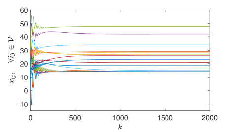
Figure 2: The agent states $x_{ij},\forall ij\in\mathcal{V}$ under the proposed algorithm (3) in Case 1.

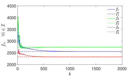
Figure 3: The values of coalition-level objective functions $f_{i}(\bm{x}),\forall i\in\mathcal{I}$ under the proposed algorithm (3) in Case 1.

Figure 4: The sum of agent states within each coalition $\sum_{ij\in\mathcal{V}_{i}}x_{ij},\forall i\in\mathcal{I}$ under the proposed algorithm (3) in Case 1 .

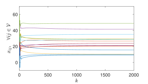
Figure 5: The agent states $x_{ij},\forall ij\in\mathcal{V}$ under the proposed algorithm (15) in Case 2.

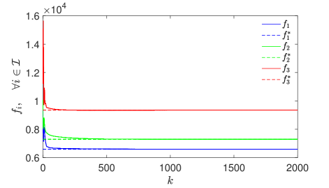
Figure 6: The values of coalition-level objective functions $f_{i}(\bm{x}),\forall i\in\mathcal{I}$ under the proposed algorithm (15) in Case 2.

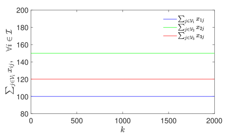
Figure 7: The sum of agent states within each coalition $\sum_{ij\in\mathcal{V}_{i}}x_{ij},\forall i\in\mathcal{I}$ under the proposed algorithm (15) in Case 2 .

Numerical examples are provided in this section to test the effectiveness of the proposed algorithms. Consider three coalitions that contain four, five and six agents respectively, i.e., $N=3$, $\mathcal{I}=\{1,2,3\}$, $n_{1}=4$, $n_{2}=5$, $n_{3}=6$. The network topology is shown in Fig. 1. In the following, we consider two cases that can be described by model (1) and (2) respectively.

In Case 1, the objective function of each agent $ij\in\mathcal{V}$ is

$$f_{ij}(x_{ij},\bm{x}_{-i})=(x_{ij}-b_{ij})^{2}{+}\frac{1}{2}x_{ij}y_{ij},$$

where $y_{11}{=}x_{31},~{}y_{12}{=}x_{21}+x_{32},~{}y_{13}{=}x_{22}+x_{33},~{}y_{14}{=}x_{23}+x_{34},~{}y_{21}{=}x_{12}+x_{32},~{}y_{22}{=}x_{13}+x_{33},~{}y_{23}{=}x_{14}+x_{34},~{}y_{24}{=}x_{35},~{}y_{25}{=}x_{36},~{}y_{31}{=}x_{11},~{}y_{32}{=}x_{12}+x_{21},~{}y_{33}{=}x_{13}+x_{22},~{}y_{34}{=}x_{14}+x_{23},~{}y_{35}{=}x_{24},~{}y_{36}{=}x_{25}$, and $b_{11}{=}20$, $b_{12}{=}30$, $b_{13}{=}40$, $b_{14}{=}50$, $b_{21}{=}50$, $b_{22}{=}40$, $b_{23}{=}30$, $b_{24}{=}20$, $b_{25}{=}30$, $b_{31}{=}b_{32}{=}b_{33}{=}b_{34}{=}b_{35}{=}b_{36}{=}20$. The quantities of resources in the three coalitions are $R_{1}=100$, $R_{2}=150$, and $R_{3}=120$, respectively. Note that in this case, the inputs of the individual objective function for each agent include only the states of itself and agents in other coalitions. One can directly calculate out the NE $\bm{x}^{*}{=}[14.12$, $15.29$, $28.63$, $41.96$, $47.44$, $34.11$, $20.78$, $18.5$, $29.17$, $26.89$, $14.73$, $14.73$, $14.73$, $25.79$, $23.12]^{T}$ and the values of the coalition-level objective functions at the NE $f_{1}^{*}{=}2554,~{}f_{2}^{*}{=}2746,~{}f_{3}^{*}{=}2326$. The initial collective state is $\bm{x}(0){=}[25,25,25,25,30,30,30,30,30,20,20,20,20,20,20]^{T}$. We employ the proposed algorithm (3) for the special case with the algorithm parameter set as $\alpha{=}0.02$. The simulation result is presented in Figs. 2-4, which show that the agent states converge fast to the NE and the resource constraints are satisfied during the whole process.

In Case 2, the objective function of each agent $ij\in\mathcal{V}$ is

$$f_{ij}(\bm{x})=5(x_{ij}-d_{ij})^{2}{+}\frac{1}{2}x_{ij}y_{ij},$$

where $y_{11}{=}x_{12}+x_{21}+x_{31}+x_{32},~{}y_{12}{=}x_{11}+x_{21}+x_{31}+x_{32},~{}y_{13}{=}x_{22}+x_{23}+x_{33}+x_{34},~{}y_{14}{=}x_{24}+x_{25}+x_{35}+x_{36},~{}y_{21}{=}x_{11}+x_{12}+x_{31}+x_{32},~{}y_{22}{=}x_{13}+x_{23}+x_{33}+x_{34},~{}y_{23}{=}x_{13}+x_{22}+x_{33}+x_{34},~{}y_{24}{=}x_{14}+x_{25}+x_{35}+x_{36},~{}y_{25}{=}x_{14}+x_{24}+x_{35}+x_{36},~{}y_{31}{=}x_{11}+x_{12}+x_{21}+x_{32},~{}y_{32}{=}x_{11}+x_{12}+x_{21}+x_{31},~{}y_{33}{=}x_{13}+x_{22}+x_{23}+x_{34},~{}y_{34}{=}x_{13}+x_{22}+x_{23}+x_{33},~{}y_{35}{=}x_{14}+x_{24}+x_{25}+x_{36},~{}y_{36}{=}x_{14}+x_{24}+x_{25}+x_{35}$, and $d_{11}{=}20$, $d_{12}{=}30$, $d_{13}{=}40$, $d_{14}{=}50$, $d_{21}{=}50$, $d_{22}{=}40$, $d_{23}{=}30$, $d_{24}{=}20$, $d_{25}{=}30$, $d_{31}{=}d_{36}{=}20$, $d_{32}{=}d_{35}{=}30$, $d_{33}{=}d_{34}{=}40$. The quantities of resources in the three coalitions are the same as in Case 1. By direct calculation, one can obtain the NE $\bm{x}^{*}{=}[9.08$, $20.19$, $29.27$, $41.46$, $48.78$, $35.07$, $23.96$, $15.54$, $26.65$, $10.14$, $21.25$, $28.87$, $28.87$, $21.0$, $9.89]^{T}$, and the values of the coalition-level objective functions at the NE are $f_{1}^{*}{=}6598,~{}f_{2}^{*}{=}7295,~{}f_{3}^{*}=9347$, respectively. The proposed algorithm (15) for the general case is employed with the algorithm parameter set as $\beta{=}0.01$, and the simulation results are presented in Figs. 5-7, showing that the agent states achieve fast convergence to the NE while satisfying the resource constraints.

6 Conclusion

In this paper, the problem of distributed resource allocation over multiple interacting coalitions is investigated by developing game-theoretic approaches. To characterize the cooperation of individual agents on resource allocation in each coalition as well as the conflicts of interest among different coalitions, a new type of multi-coalition game is formulated. Inspired by techniques such as variable replacement, gradient tracking and leader-following consensus, two new kinds of DRA algorithms are developed respectively for the scenarios where the individual benefit of each agent explicitly depends on the states of itself and some agents in other coalitions, and on the states of all the game participants. One favourable feature of the designed DRA algorithms is that the resource constraints can be satisfied during the whole allocation process. Furthermore, linear convergence of the proposed DRA algorithms is successfully established. In the future, we will consider the cases with directed topologies and time-varying objective functions.

.1 Proof of Lemma 2

From (9), one has

$$V_{\xi}({k{+}1}){{-}}V_{\xi}(k)$$

$${=} \bm{e_{\xi}}^{T}(t_{k})(\mathcal{M}^{T}W_{\mathcal{M}}\mathcal{M}{{-}}W_{\mathcal{M}})\bm{e_{\xi}}(t_{k})$$

$${{+}}2\bm{e_{\xi}}^{T}(t_{k})\mathcal{M}^{T}W_{\mathcal{M}}(\bm{1}_{n_{\mathrm{sum}}}{{\otimes}}(\alpha\hat{L}^{2}\breve{\mathcal{P}}(\bm{\xi}({k}))))$$

$${{+}}(\bm{1}_{n_{\mathrm{sum}}}{{\otimes}}(\alpha\hat{L}^{2}\breve{\mathcal{P}}(\bm{\xi}({k}))))^{T}W_{\mathcal{M}}(\bm{1}_{n_{\mathrm{sum}}}{{\otimes}}(\alpha\hat{L}^{2}\breve{\mathcal{P}}(\bm{\xi}({k}))))$$

$${\leq} {{-}}\|\bm{e_{\xi}}(k)\|^{2}{{+}}2\sqrt{n_{\mathrm{sum}}}\|\mathcal{M}^{T}W_{\mathcal{M}}\|\|\bm{e_{\xi}}(k)\|\|\alpha\hat{L}^{2}\breve{\mathcal{P}}(\bm{\xi}({k}))\|$$

$${{+}}n_{\mathrm{sum}}\|W_{\mathcal{M}}\|\|\alpha\hat{L}^{2}\breve{\mathcal{P}}(\bm{\xi}({k}))\|^{2}$$

$${\leq} {{-}}\frac{1}{2}\|\bm{e_{\xi}}(k)\|^{2}{{+}}\alpha^{2}b\|\hat{L}^{2}\breve{\mathcal{P}}(\bm{\xi}({k}))\|^{2}.$$

.2 Proof of Lemma 3

First, one can easily obtain

$$\left\|L_{i}\frac{\partial f_{i}}{\partial\bm{x}_{i}}(\bm{x}(k+1))\right\|^{2}{-}\left\|L_{i}\frac{\partial f_{i}}{\partial\bm{x}_{i}}(\bm{x}(k))\right\|^{2}$$ (33)

$$= \left\|L_{i}\frac{\partial f_{i}}{\partial\bm{x}_{i}}(\bm{x}(k+1)){-}L_{i}\frac{\partial f_{i}}{\partial\bm{x}_{i}}(\bm{x}(k))\right\|^{2}$$

$${+}2\left(L_{i}\frac{\partial f_{i}}{\partial\bm{x}_{i}}(\bm{x}(k+1)){-}L_{i}\frac{\partial f_{i}}{\partial\bm{x}_{i}}(\bm{x}(k))\right)^{T}$$

$$\times L_{i}\frac{\partial f_{i}}{\partial\bm{x}_{i}}(\bm{x}(k)).$$

From (6), one can derive that

$$2\left(L_{i}\frac{\partial f_{i}}{\partial\bm{x}_{i}}(\bm{x}(k+1)){-}L_{i}\frac{\partial f_{i}}{\partial\bm{x}_{i}}(\bm{x}(k))\right)^{T}L_{i}\frac{\partial f_{i}}{\partial\bm{x}_{i}}(\bm{x}(k))$$

$$= 2\left(L_{i}\frac{\partial f_{i}}{\partial\bm{x}_{i}}(\bm{x}(k+1)){-}L_{i}\frac{\partial f_{i}}{\partial\bm{x}_{i}}(\bm{x}(k))\right)^{T}L_{i}\bigg{(}\breve{\mathcal{P}}_{i}(\bm{\xi}_{i})$$

$${+}\frac{\partial f_{i}}{\partial\bm{x}_{i}}(\bm{x}(k)){-}\breve{\mathcal{P}}_{i}(\bm{\xi}_{i})\bigg{)}$$

$$= {-}\frac{2}{\alpha}\left(\frac{\partial f_{i}}{\partial\bm{x}_{i}}(\bm{x}(k+1)){-}\frac{\partial f_{i}}{\partial\bm{x}_{i}}(\bm{x}(k))\right)^{T}\left({\bm{x}}_{i}(k{{+}}1){{-}}{\bm{x}}_{i}(k)\right)$$

$${+}2\left(L_{i}\frac{\partial f_{i}}{\partial\bm{x}_{i}}(\bm{x}(k+1)){-}L_{i}\frac{\partial f_{i}}{\partial\bm{x}_{i}}(\bm{x}(k))\right)^{T}$$

$$\times L_{i}\bigg{(}\frac{\partial f_{i}}{\partial\bm{x}_{i}}(\bm{x}(k)){-}\breve{\mathcal{P}}_{i}(\bm{\xi}_{i})\bigg{)}$$

$$\leq {-}\frac{2}{\alpha}\left(\frac{\partial f_{i}}{\partial\bm{x}_{i}}(\bm{x}(k+1)){-}\frac{\partial f_{i}}{\partial\bm{x}_{i}}(\bm{x}(k))\right)^{T}\left({\bm{x}}_{i}(k{{+}}1){{-}}{\bm{x}}_{i}(k)\right)$$

$${+}\left\|L_{i}\frac{\partial f_{i}}{\partial\bm{x}_{i}}(\bm{x}(k+1)){-}L_{i}\frac{\partial f_{i}}{\partial\bm{x}_{i}}(\bm{x}(k))\right\|^{2}$$

$${+}\left\|L_{i}\bigg{(}\frac{\partial f_{i}}{\partial\bm{x}_{i}}(\bm{x}(k)){-}\breve{\mathcal{P}}_{i}(\bm{\xi}_{i})\bigg{)}\right\|^{2}.$$

Note that under Assumption 1, one has

$$\left\|\breve{\mathcal{P}}_{i}(\bm{\xi}_{i}(k)){{-}}\frac{\partial f_{i}}{\partial\bm{x}_{i}}(\bm{x}(k))\right\|$$ (34)

$$= \sqrt{\sum\limits_{j=1}^{n_{i}}\bigg{(}\frac{\partial f_{i}}{\partial{x}_{ij}}(\bm{\xi}_{ij}(k)){{-}}\frac{\partial f_{i}}{\partial{x}_{ij}}(\bm{x}(k))\bigg{)}^{2}}$$

$$\leq \sqrt{\sum\limits_{j=1}^{n_{i}}\big{\|}\nabla f_{i}(\bm{\xi}_{ij}(k)){{-}}\nabla f_{i}(\bm{x}(k))\big{\|}^{2}}$$

$$\leq l_{i}\left\|\bm{\xi}_{i}(k){{-}}\bm{1}_{n_{i}}{\otimes}\bm{x}(k)\right\|.$$

Combining the above three formulas yields

$$V_{x}(k{{+}}1){-}V_{x}(k)$$

$$\leq {-}\frac{2}{\alpha}(\mathcal{P}(\bm{x}(k{{+}}1)){-}\mathcal{P}(\bm{x}(k)))^{T}({\bm{x}}(k{{+}}1){-}{\bm{x}}(k))$$

$${+}2\sum_{i=1}^{N}\left\|L_{i}\frac{\partial f_{i}}{\partial\bm{x}_{i}}(\bm{x}(k+1)){-}L_{i}\frac{\partial f_{i}}{\partial\bm{x}_{i}}(\bm{x}(k))\right\|^{2}$$

$${+}\sum_{i=1}^{N}\left\|L_{i}\bigg{(}\frac{\partial f_{i}}{\partial\bm{x}_{i}}(\bm{x}(k)){-}\breve{\mathcal{P}}_{i}(\bm{\xi}_{i})\bigg{)}\right\|^{2}$$

$$\leq {-}\frac{2\mu}{\alpha}\left\|{\bm{x}}(k{{+}}1){{-}}{\bm{x}}(k)\right\|^{2}$$

$${+}2\sum_{i=1}^{N}\Big{(}l_{i}^{2}\|L_{i}\|^{2}\|{\bm{x}}(k{{+}}1){{-}}{\bm{x}}(k)\|^{2}\Big{)}$$

$${+}\sum_{i=1}^{N}\Big{(}l_{i}^{2}\left\|L_{i}\right\|^{2}\left\|\bm{\xi}_{i}(k){{-}}\bm{1}_{n_{i}}{\otimes}\bm{x}(k)\right\|^{2}\Big{)}$$

$$\leq {-}2\Big{(}{\mu}{-}{\alpha}\sum_{i=1}^{N}(l_{i}^{2}\|L_{i}\|^{2})\Big{)}\alpha\left\|\hat{L}^{2}\breve{\mathcal{P}}(\bm{\xi}({k}))\right\|^{2}$$

$${+}\max_{i\in\mathcal{I}}\{l_{i}^{2}\|L_{i}\|^{2}\}\left\|\bm{e_{\xi}}(k)\right\|^{2},$$

which completes the proof.

.3 Proof of Lemma 5

One can derive from the iteration of $\bm{e_{\psi_{i}}}$ in (24) that

$$V_{\psi}(k{{+}}1){{-}}V_{\psi}(k)$$

$$= \sum_{i=1}^{N}\bigg{(}\bm{e_{\psi_{i}}}^{T}(k)\big{(}(\bar{C}_{i}^{T}W_{c_{i}}\bar{C}_{i}{-}W_{c_{i}}){{\otimes}}I_{n_{i}}\big{)}\bm{e_{\psi_{i}}}(k)$$

$${+}2\bm{e_{\psi_{i}}}^{T}(k)(\bar{C}_{i}^{T}W_{c_{i}}\bar{I}_{i}{{\otimes}}I_{n_{i}})\left(\mathcal{Q}_{i}(\bm{\xi}_{i}(k{{+}}1)){{-}}\mathcal{Q}_{i}(\bm{\xi}_{i}({k}))\right)$$

$${+}\left(\mathcal{Q}_{i}(\bm{\xi}_{i}(k{{+}}1)){{-}}\mathcal{Q}_{i}(\bm{\xi}_{i}({k}))\right)^{T}(\bar{I}_{i}^{T}W_{c_{i}}\bar{I}_{i}{{\otimes}}I_{n_{i}})$$

$${\times}\left(\mathcal{Q}_{i}(\bm{\xi}_{i}(k{{+}}1)){{-}}\mathcal{Q}_{i}(\bm{\xi}_{i}({k}))\right)\bigg{)}$$

$${\leq} \sum_{i=1}^{N}\bigg{(}{-}\|\bm{e_{\psi_{i}}}(k)\|^{2}{+}\frac{1}{2}\|\bm{e_{\psi_{i}}}(k)\|^{2}$$

$${+}2\|\bar{C}_{i}^{T}W_{c_{i}}\bar{I}_{i}\|^{2}\|\mathcal{Q}_{i}(\bm{\xi}_{i}(k{{+}}1)){{-}}\mathcal{Q}_{i}(\bm{\xi}_{i}({k}))\|^{2}$$

$${+}\|\bar{I}_{i}^{T}W_{c_{i}}\bar{I}_{i}\|\|\mathcal{Q}_{i}(\bm{\xi}_{i}(k{{+}}1)){{-}}\mathcal{Q}_{i}(\bm{\xi}_{i}({k}))\|^{2}\bigg{)}$$

$$= {{-}}\frac{1}{2}\|\bm{e_{\psi}}(k)\|^{2}{+}\sum_{i=1}^{N}(2\|\bar{C}_{i}^{T}W_{c_{i}}\bar{I}_{i}\|^{2}{+}\|\bar{I}_{i}^{T}W_{c_{i}}\bar{I}_{i}\|)$$

$$\times\|\mathcal{Q}_{i}(\bm{\xi}_{i}(k{{+}}1)){{-}}\mathcal{Q}_{i}(\bm{\xi}_{i}({k}))\|^{2}.$$

Under Assumption 1, one has

$$\left\|\mathcal{Q}_{i}(\bm{\xi}_{i}(k{{+}}1)){{-}}\mathcal{Q}_{i}(\bm{\xi}_{i}({k}))\right\|^{2}{\leq}\max_{ij\in\mathcal{V}_{i}}\{l_{ij}^{2}\}\left\|\bm{\xi}_{i}(k{{+}}1){{-}}\bm{\xi}_{i}({k})\right\|^{2}.$$

Combining the above inequalities yields

$$V_{\psi}(k{{+}}1){{-}}V_{\psi}(k)$$

$${\leq} {{-}}\frac{1}{2}\|\bm{e_{\psi}}(k)\|^{2}{+}\sum_{i=1}^{N}(2\|\bar{C}_{i}^{T}W_{c_{i}}\bar{I}_{i}\|^{2}{+}\|\bar{I}_{i}^{T}W_{c_{i}}\bar{I}_{i}\|)$$

$$\times\max_{ij\in\mathcal{V}_{i}}\{l_{ij}^{2}\}\|\bm{\xi}_{i}(k{{+}}1){{-}}\bm{\xi}_{i}({k})\|^{2}$$

$${\leq} {{-}}\frac{1}{2}\|\bm{e_{\psi}}(k)\|^{2}{+}\max_{i\in\mathcal{I},ij\in\mathcal{V}_{i}}\{(2\|\bar{C}_{i}^{T}W_{c_{i}}\bar{I}_{i}\|^{2}{+}\|\bar{I}_{i}^{T}W_{c_{i}}\bar{I}_{i}\|)l_{ij}^{2}\}$$

$$\times\|\bm{\xi}(k{{+}}1){{-}}\bm{\xi}({k})\|^{2}$$

$${\leq} {{-}}\frac{1}{2}\|\bm{e_{\psi}}(k)\|^{2}{+}2\max_{i\in\mathcal{I},ij\in\mathcal{V}_{i}}\{(2\|\bar{C}_{i}^{T}W_{c_{i}}\bar{I}_{i}\|^{2}{+}\|\bar{I}_{i}^{T}W_{c_{i}}\bar{I}_{i}\|)l_{ij}^{2}\}$$

$$\times\|I_{n_{\mathrm{sum}}}{{-}}\mathcal{M}\|^{2}\|\bm{e_{\xi}}(k)\|^{2},$$

where the last inequality is obtained by recalling (8), (26), and (27).

.4 Proof of Lemma 6

One can derive that

$$2\left(L_{i}\frac{\partial f_{i}}{\partial\bm{x}_{i}}(\bm{x}(k+1)){-}L_{i}\frac{\partial f_{i}}{\partial\bm{x}_{i}}(\bm{x}(k))\right)^{T}L_{i}\frac{\partial f_{i}}{\partial\bm{x}_{i}}(\bm{x}(k))$$

$$= 2\left(L_{i}\frac{\partial f_{i}}{\partial\bm{x}_{i}}(\bm{x}(k+1)){-}L_{i}\frac{\partial f_{i}}{\partial\bm{x}_{i}}(\bm{x}(k))\right)^{T}\bigg{(}n_{i}\breve{L}_{i}\bm{\psi}_{i}(k)$$

$${+}n_{i}L_{i}{\bar{{\bm{\psi}}}}_{i}(k){-}n_{i}\breve{L}_{i}\bm{\psi}_{i}(k)$$

$${+}L_{i}\frac{\partial f_{i}}{\partial\bm{x}_{i}}(\bm{x}(k)){-}n_{i}L_{i}\bar{\mathcal{Q}}_{i}(\bm{\xi}_{i}({k}))\bigg{)}$$

$$= {-}\frac{2n_{i}}{\beta}\left(\frac{\partial f_{i}}{\partial\bm{x}_{i}}(\bm{x}(k+1)){-}\frac{\partial f_{i}}{\partial\bm{x}_{i}}(\bm{x}(k))\right)^{T}\left({\bm{x}}_{i}(k{{+}}1){{-}}{\bm{x}}_{i}(k)\right)$$

$${+}2\left(L_{i}\frac{\partial f_{i}}{\partial\bm{x}_{i}}(\bm{x}(k+1)){-}L_{i}\frac{\partial f_{i}}{\partial\bm{x}_{i}}(\bm{x}(k))\right)^{T}$$

$$\times\bigg{(}L_{i}\left(\frac{\partial f_{i}}{\partial\bm{x}_{i}}(\bm{x}(k)){-}n_{i}\bar{\mathcal{Q}}_{i}(\bm{\xi}_{i}({k}))\right){-}n_{i}\breve{L}_{i}\bm{e_{\psi_{i}}}(k)\bigg{)}$$

$$\leq {-}\frac{2n_{i}}{\beta}\left(\frac{\partial f_{i}}{\partial\bm{x}_{i}}(\bm{x}(k+1)){-}\frac{\partial f_{i}}{\partial\bm{x}_{i}}(\bm{x}(k))\right)^{T}\left({\bm{x}}_{i}(k{{+}}1){{-}}{\bm{x}}_{i}(k)\right)$$

$${+}\left\|L_{i}\frac{\partial f_{i}}{\partial\bm{x}_{i}}(\bm{x}(k+1)){-}L_{i}\frac{\partial f_{i}}{\partial\bm{x}_{i}}(\bm{x}(k))\right\|^{2}$$

$${+}2\left\|L_{i}\left(\frac{\partial f_{i}}{\partial\bm{x}_{i}}(\bm{x}(k)){-}n_{i}\bar{\mathcal{Q}}_{i}(\bm{\xi}_{i}({k}))\right)\right\|^{2}{+}2\left\|n_{i}\breve{L}_{i}\bm{e_{\psi_{i}}}(k)\right\|^{2},$$

where the first equality is obtained from (17), the second equality is obtained from (16a), (16b) and (30). Combining the above formula and (33) yields

$$\left\|L_{i}\frac{\partial f_{i}}{\partial\bm{x}_{i}}(\bm{x}(k+1))\right\|^{2}{-}\left\|L_{i}\frac{\partial f_{i}}{\partial\bm{x}_{i}}(\bm{x}(k))\right\|^{2}$$

$$\leq {{-}}\frac{2n_{i}}{\beta}\left(\frac{\partial f_{i}}{\partial\bm{x}_{i}}(\bm{x}(k+1)){-}\frac{\partial f_{i}}{\partial\bm{x}_{i}}(\bm{x}(k))\right)^{T}\left({\bm{x}}_{i}(k{{+}}1){{-}}{\bm{x}}_{i}(k)\right)$$

$${{+}}2\left\|L_{i}\frac{\partial f_{i}}{\partial\bm{x}_{i}}(\bm{x}(k+1)){{-}}L_{i}\frac{\partial f_{i}}{\partial\bm{x}_{i}}(\bm{x}(k))\right\|^{2}$$

$${{+}}2\left\|L_{i}\Big{(}\frac{\partial f_{i}}{\partial\bm{x}_{i}}(\bm{x}(k)){{-}}n_{i}\bar{\mathcal{Q}}_{i}(\bm{\xi}_{i}({k}))\Big{)}\right\|^{2}{{+}}2\left\|n_{i}\breve{L}_{i}\bm{e_{\psi_{i}}}(k)\right\|^{2}.$$

Under Assumption 1, one has

$$\left\|\frac{\partial f_{i}}{\partial\bm{x}_{i}}(\bm{x}(k)){-}n_{i}\bar{\mathcal{Q}}_{i}(\bm{\xi}_{i}({k}))\right\|$$ (35)

$${\leq} \sum\limits_{j=1}^{n_{i}}\bigg{\|}\frac{\partial f_{ij}(\bm{\xi}_{ij}(k))}{\partial\bm{x}_{i}}{{-}}\frac{\partial f_{ij}(\bm{{x}}(k))}{\partial\bm{x}_{i}}\bigg{\|}$$

$${\leq} \sum\limits_{j=1}^{n_{i}}l_{ij}\|\bm{\xi}_{ij}(k){{-}}\bm{{x}}(k)\|$$

$$\leq \sqrt{\sum_{j=1}^{n_{i}}l_{ij}^{2}}\cdot\big{\|}\bm{e_{\xi_{i}}}(k)\big{\|}.$$

Based on the above formulas, the following can be derived:

$$\bar{V}_{x}(k{{+}}1){-}\bar{V}_{x}(k)$$

$$\leq {{-}}\frac{1}{\beta}\sum_{i=1}^{N}\left(\frac{\partial f_{i}}{\partial\bm{x}_{i}}(\bm{x}(k+1)){{-}}\frac{\partial f_{i}}{\partial\bm{x}_{i}}(\bm{x}(k))\right)^{T}\left({\bm{x}}_{i}(k{{+}}1){{-}}{\bm{x}}_{i}(k)\right)$$

$${+}\sum_{i=1}^{N}\frac{1}{n_{i}}\bigg{(}\left\|L_{i}\frac{\partial f_{i}}{\partial\bm{x}_{i}}(\bm{x}(k+1)){{-}}L_{i}\frac{\partial f_{i}}{\partial\bm{x}_{i}}(\bm{x}(k))\right\|^{2}$$

$${+}\left\|L_{i}\left(\frac{\partial f_{i}}{\partial\bm{x}_{i}}(\bm{x}(k)){{-}}n_{i}\bar{\mathcal{Q}}_{i}(\bm{\xi}_{i}({k}))\right)\right\|^{2}{+}\left\|n_{i}\breve{L}_{i}\bm{e_{\psi_{i}}}(k)\right\|^{2}\bigg{)}$$

$$\leq {{-}}\frac{\mu}{\beta}\left\|{\bm{x}}(k{{+}}1){{{-}}}{\bm{x}}(k)\right\|^{2}{+}\sum_{i=1}^{N}\frac{1}{n_{i}}\bigg{(}l_{i}^{2}\|L_{i}\|^{2}\left\|{\bm{x}}(k{{+}}1){{-}}{\bm{x}}(k)\right\|^{2}$$

$${+}(\sum_{j=1}^{n_{i}}l_{ij}^{2})\left\|L_{i}\right\|^{2}\big{\|}\bm{e_{\xi_{i}}}(k)\big{\|}^{2}{+}n_{i}^{2}\|\breve{L}_{i}\|^{2}\left\|\bm{e_{\psi_{i}}}(k)\right\|^{2}\bigg{)}$$

$$\leq {{-}}(\frac{\mu}{\beta}{{-}}\sum_{i=1}^{N}\frac{l_{i}^{2}\|L_{i}\|^{2}}{n_{i}})\beta^{2}\left\|\hat{L}\hat{\breve{L}}\bm{\psi}({k})\right\|^{2}$$

$${+}\max_{i\in\mathcal{I}}\Big{\{}\frac{1}{n_{i}}(\sum_{j=1}^{n_{i}}l_{ij}^{2})\left\|L_{i}\right\|^{2}\Big{\}}\left\|\bm{e_{\xi}}(k)\right\|^{2}$$

$${+}\max_{i\in\mathcal{I}}\{n_{i}\|\breve{L}_{i}\|^{2}\}\left\|\bm{e_{\psi}}(k)\right\|^{2},$$

which completes the proof.

References

- [1] T. Yang, X. Yi, J. Wu, Y. Yuan, D. Wu, Z. Meng, Y. Hong, H. Wang, Z. Lin, and K. H. Johansson, “A survey of distributed optimization,” Annual Reviews in Control, vol. 47, pp. 278–305, 2019.
- [2] T. Yang, J. Lu, D. Wu, J. Wu, G. Shi, Z. Meng, and K. H. Johansson, “A distributed algorithm for economic dispatch over time-varying directed networks with delays,” IEEE Trans. Ind. Electron., vol. 64, no. 6, pp. 5095–5106, Jun. 2017.
- [3] F. Guo, C. Wen, J. Mao, J. Chen, and Y. Song, “Hierarchical decentralized optimization architecture for economic dispatch: a new approach for large-scale power system,” IEEE Trans. Ind. Informat., vol. 14, no. 2, pp. 523–534, Feb. 2018.
- [4] G. Binetti, A. Davoudi, F. L. Lewis, D. Naso, and B. Turchiano, “Distributed consensus-based economic dispatch with transmission losses,” IEEE Trans. Power Syst., vol. 29, no. 4, pp. 1711–1720, Jul. 2014.
- [5] A. Beck, A. Nedić, A. Ozdaglar, and M. Teboulle, “An gradient method for network resource allocation problems,” IEEE Control Netw. Syst., vol. 1, no. 1, pp. 64–73, Mar. 2014.
- [6] E. Ghadimi, I. Shames, and M. Johansson, “Multi-step gradient methods for networked optimization,” IEEE Trans. Signal Process., vol. 61, no. 21, pp. 5417–5429, Nov. 2013.
- [7] M. Zargham, A. Ribeiro, A. Ozdaglar, and A. Jadbabaie, “Accelerated dual descent for network flow optimization,” IEEE Trans. Autom. Control, vol. 59, no. 4, pp. 905–920, Apr. 2014.
- [8] T. Yang, D. Wu, Y. Sun, and J. Lian, “Minimum-time consensus based approach for power system applications,”IEEE Trans. Ind. Electron., vol. 63, no. 2, pp. 1318–1328, Feb. 2016.
- [9] A. Cherukuri and J. Cortés, “Initialization-free distributed coordination for economic dispatch under varying loads and generator commitment,” Automatica, vol. 74, pp. 183–193, Dec. 2016.
- [10] G. Wen, X. Yu, Z. Liu, and W. Yu, “Adaptive consensus-based robust strategy for economic dispatch of smart grids subject to communication uncertainties,” IEEE Trans. Ind. Informat., vol. 14, no. 6, pp. 2484–2496, Jun. 2018.
- [11] Y. Zhu, G. Wen, W. Yu, and X. Yu, “Continuous-time distributed proximal gradient algorithms for nonsmooth resource allocation over general digraphs,” IEEE Trans. Netw. Sci. Eng., vol. 8, no. 2, pp. 1733–1744, Apr.-Jun. 2021.
- [12] G. Chen and Z. Li, “A fixed-time convergent algorithm for distributed convex optimization in multi-agent systems,” Automatica, vol. 95, pp. 539–543, Sep. 2018.
- [13] J. Zhou, Y. Lv, C. Wen, and G. Wen, “Solving specified-time distributed optimization problem via sampled-data-based algorithm,” arXiv preprint, arXiv:2106.11684.
- [14] Z. Guo and G. Chen, “Predefined-time distributed optimal allocation of resources: a time-base generator scheme,” IEEE Trans. Syst., Man, Cybern. Syst., vol. 52, no. 1, pp. 438–447, Jan. 2022.
- [15] B. Gharesifard and J. Cortés, “Distributed convergence to Nash equilibria in two-network zero-sum games,” Automatica, vol. 49, no. 6, pp. 1683–1692, Jun. 2013.
- [16] Y. Lou, Y. Hong, L. Xie, G. Shi, and K. H. Johansson, “Nash equilibrium computation in subnetwork zero-sum games with switching communications,” IEEE Trans. Autom. Control, vol. 61, no. 10, pp. 2920–2935, Oct. 2016.
- [17] M. Ye, G. Hu, and F. L. Lewis, “Nash equilibrium seeking for N-coalition noncooperative games,” Automatica, vol. 95, pp. 266–272, Sep. 2018.
- [18] X. Nian, F. Niu, and Z. Yang, “Distributed Nash equilibrium seeking for multicluster game under switching communication topologies,” IEEE Trans. Syst., Man, Cybern. Syst., doi: 10.1109/TSMC.2021.3090515.
- [19] Y. Pang and G. Hu, “Nash equilibrium seeking in N-coalition games via a gradient-free method,” Automatica, vol. 136, pp. 110013, Feb. 2022.
- [20] X. Zeng, J. Chen, S. Liang, and Y. Hong, “Generalized Nash equilibrium seeking strategy for distributed nonsmooth multi-cluster game,” Automatica, vol. 103, pp. 20–26, May 2019.
- [21] M. Meng and X. Li, “On the linear convergence of distributed Nash equilibrium seeking for multi-cluster games under partial-decision information,” arXiv e-prints, arXiv:2005.06923, May 2020.
- [22] J. Zhou, Y. Lv, G. Wen, J. Lü, and D. Zheng, “Distributed Nash equilibrium seeking in consistency-constrained multi-coalition games,” IEEE Trans. Cybern., doi: 10.1109/TCYB.2022.3155687.
- [23] M. S. Bazaraa, H. D. Sherali, and C. M. Shetty, Nonlinear Programming: Theory and Algorithms, 3rd Edition, Hoboken, NJ, USA: John Wiley & Sons, Inc., 2006.
- [24] A. Nedić, A. Olshevsky, and W. Shi, “Achieving geometric convergence for distributed optimization over time-varying graphs,” SIAM J. Optim., vol. 27, no. 4, pp. 2597–2633, 2017.