Exploring the electromagnetic properties of the $\Xi_{c}^{(\prime,\,*)}\bar{D}_{s}^{*}$ and $\Omega_{c}^{(*)}\bar{D}_{s}^{*}$ molecular states

Abstract

This paper presents a systematic investigation of the electromagnetic properties of the hidden-charm molecular pentaquarks within the constituent quark model. Specifically, it focuses on two types of pentaquarks: the $\Xi_{c}^{(\prime,*)}\bar{D}_{s}^{*}$-type pentaquarks with double strangeness and the $\Omega_{c}^{(*)}\bar{D}_{s}^{*}$-type pentaquarks with triple strangeness. The study explores various electromagnetic properties, including the magnetic moments, the transition magnetic moments, and the radiative decay behavior of these pentaquarks. To ensure realistic calculations, the $S$-$D$ wave mixing effect and the coupled channel effect are taken into account. By examining the electromagnetic properties of the hidden-charm molecular pentaquarks with double and triple strangeness, this research contributes to the deeper understanding of their spectroscopic behavior. These findings form a valuable addition to the ongoing investigation into the broader spectrum of properties exhibited by the hidden-charm molecular pentaquarks.

I Introduction

Since the observation of the charmoniumlike state $X(3872)$ in 2003, numerous new hadronic states have been experimentally observed, leading to extensive discussions about their properties. These efforts have significantly enriched our understanding of the hadron spectroscopy Liu:2013waa ; Hosaka:2016pey ; Chen:2016qju ; Richard:2016eis ; Lebed:2016hpi ; Olsen:2017bmm ; Guo:2017jvc ; Brambilla:2019esw ; Liu:2019zoy ; Chen:2022asf ; Meng:2022ozq ; Amsler:2004ps ; Swanson:2006st ; Godfrey:2008nc ; Yamaguchi:2019vea ; Albuquerque:2018jkn ; Yuan:2018inv ; Ali:2017jda ; Dong:2017gaw ; Faccini:2012pj ; Drenska:2010kg ; Pakhlova:2010zza . Moreover, these studies have been valuable in deepening our understanding of the nonperturbative behavior of the strong interactions.

Among the various assignments proposed for the observed new hadronic states, the molecular state explanation has gained popularity. Notably, in 2015, the LHCb Collaboration observed two $P_{c}$ states Aaij:2015tga and subsequently reported two substructures, namely $P_{c}(4440)$ and $P_{c}(4457)$ Aaij:2019vzc , corresponding to the previously observed $P_{c}(4450)$ Aaij:2015tga . Furthermore, they discovered a new state, $P_{c}(4312)$, through a detailed analysis of the $\Lambda_{b}\to J/\psi pK$ process Aaij:2019vzc . The LHCb experiment has provided strong experimental evidence for the existence of the hidden-charm molecular pentaquarks of the $\Sigma_{c}\bar{D}^{(*)}$ type Wu:2010jy ; Wang:2011rga ; Yang:2011wz ; Wu:2012md ; Li:2014gra ; Karliner:2015ina ; Chen:2015loa . In subsequent years, LHCb reported the evidence for $P_{cs}(4459)$ LHCb:2020jpq and observed $P_{\psi s}^{\Lambda}(4338)$ LHCb:2022jad . These exciting experimental advancements have not only enriched the hidden-charm pentaquark family Hofmann:2005sw ; Wu:2010vk ; Anisovich:2015zqa ; Wang:2015wsa ; Feijoo:2015kts ; Chen:2015sxa ; Chen:2016ryt ; Lu:2016roh ; Xiao:2019gjd ; Shen:2020gpw ; Zhang:2020cdi ; Wang:2019nvm ; Weng:2019ynv ; Chen:2020uif ; Peng:2020hql ; Chen:2020opr ; Liu:2020hcv ; Dong:2021juy ; Chen:2022onm ; Chen:2020kco ; Chen:2021cfl ; Chen:2021spf ; Du:2021bgb ; Hu:2021nvs ; Xiao:2021rgp ; Zhu:2021lhd ; Wang:2022neq ; Wang:2022mxy ; Karliner:2022erb ; Yan:2022wuz ; Meng:2022wgl ; Azizi:2021utt ; Chen:2021tip ; Clymton:2021thh ; Zou:2021sha ; Lu:2021irg ; Ferretti:2021zis ; Paryev:2022zdx ; Nakamura:2022jpd; Giachino:2022pws ; Marse-Valera:2022khy ; Ortega:2022uyu ; Chen:2022wkh ; Zhu:2022wpi ; Yang:2022ezl ; Garcilazo:2022edi ; Feijoo:2022rxf , but have also inspired theorists to investigate the hidden-charm molecular pentaquarks of the $P_{css(s)}$ type Wang:2020bjt ; Wang:2021hql ; Azizi:2021pbh ; Azizi:2022qll . In recent years, the Lanzhou group has conducted extensive studies on the mass spectra of the hidden-charm molecular pentaquarks with double and triple strangeness. Specifically, their investigations have focused on the $\Xi_{c}^{(\prime,*)}\bar{D}_{s}^{(*)}$ Wang:2020bjt and $\Omega_{c}^{(*)}\bar{D}_{s}^{(*)}$ Wang:2021hql interactions. These studies have provided valuable insights into the properties and characteristics of these exotic hadronic states.

Currently, the investigation of the properties of the hidden-charm molecular pentaquarks remains a fascinating and significant research topic in hadron physics. It offers valuable insights for constructing a comprehensive family of the hidden-charm molecular pentaquarks. The study of the electromagnetic properties serves as an effective approach to unveil the inner structures of hadrons. A notable example is the successful application of the constituent quark model in describing the magnetic moments of the decuplet and octet baryons Schlumpf:1993rm ; Kumar:2005ei ; Ramalho:2009gk , with corresponding experimental data available Workman:2022ynf .

Given the importance of the electromagnetic properties, it is crucial to investigate the electromagnetic characteristics of the hidden-charm molecular pentaquarks. Some discussions on the electromagnetic properties of the $\Sigma_{c}^{(*)}\bar{D}^{(*)}$-type and $\Xi_{c}^{(\prime,*)}\bar{D}^{(*)}$-type hidden-charm molecular pentaquarks have been conducted within the constituent quark model Wang:2016dzu ; Gao:2021hmv ; Li:2021ryu ; Wang:2022tib . These studies shed light on the inner structures of the discussed hidden-charm molecular pentaquarks. However, it is important to note that the exploration of the electromagnetic properties for the hidden-charm molecular pentaquarks is still in its early stages. Thus, further efforts are required to obtain a comprehensive understanding of the electromagnetic properties of various types of hidden-charm molecular pentaquarks.

In this study, our focus is on investigating the electromagnetic properties of the hidden-charm molecular pentaquarks with double strangeness, specifically the $\Xi_{c}^{(\prime,*)}\bar{D}_{s}^{*}$-type pentaquarks, as well as those with triple strangeness, namely the $\Omega_{c}^{(*)}\bar{D}_{s}^{*}$-type pentaquarks. These particular pentaquark states were initially predicted in Refs. Wang:2020bjt ; Wang:2021hql . Within the framework of the constituent quark model, we examine their magnetic moments, transition magnetic moments, and radiative decay behavior. Our realistic calculations incorporate the effects of the $S$-$D$ wave mixing and coupled channels. By undertaking this investigation, we aim to enhance our understanding of the electromagnetic properties of the hidden-charm molecular pentaquarks with double and triple strangeness, thereby contributing to the comprehensive knowledge of these intriguing exotic hadrons Wang:2020bjt ; Wang:2021hql .

The structure of this paper is as follows. In Sec. II, we provide a detailed explanation of the methodology employed for calculating the electromagnetic properties of the hadronic molecules. Additionally, we present the electromagnetic properties of the $\Xi_{c}^{(\prime,*)}\bar{D}_{s}^{*}$ molecular states. In Sec. III, we shift our focus to the electromagnetic properties of the $\Omega_{c}^{(*)}\bar{D}_{s}^{*}$ molecular states. Finally, we offer a concise summary of our findings in Sec. IV.

II The electromagnetic properties of the $\Xi_{c}^{(\prime,*)}\bar{D}_{s}^{*}$ molecules

In this section, we thoroughly investigate the electromagnetic properties of two molecular states: the $\Xi_{c}^{\prime}\bar{D}_{s}^{*}$ state with $I(J^{P})=1/2({3}/{2}^{-})$ and the $\Xi_{c}^{*}\bar{D}_{s}^{*}$ state with $I(J^{P})=1/2({5}/{2}^{-})$ Wang:2020bjt . Specifically, we analyze their magnetic moments, transition magnetic moments, and radiative decay behavior. These investigations yield valuable insights into the inner structures of these states, offering significant information in this regard.

II.1 The magnetic moments and the transition magnetic moments of the $\Xi_{c}^{(\prime,*)}\bar{D}_{s}^{*}$ molecules

In the context of the constituent quark model, the hadronic magnetic moment encompasses two key components: the spin magnetic moment and the orbital magnetic moment. Specifically, when considering the $z$-component of the spin magnetic moment operator for a given hadron, denoted as $\hat{\mu}_{z}^{\rm spin}$, it can be mathematically represented as follows Liu:2003ab ; Huang:2004tn ; Zhu:2004xa ; Haghpayma:2006hu ; Wang:2016dzu ; Deng:2021gnb ; Gao:2021hmv ; Li:2021ryu ; Zhou:2022gra ; Wang:2022tib ; Li:2021ryu ; Schlumpf:1992vq ; Schlumpf:1993rm ; Cheng:1997kr ; Ha:1998gf ; Ramalho:2009gk ; Girdhar:2015gsa ; Menapara:2022ksj ; Mutuk:2021epz ; Menapara:2021vug ; Menapara:2021dzi ; Gandhi:2018lez ; Dahiya:2018ahb ; Kaur:2016kan ; Thakkar:2016sog ; Shah:2016vmd ; Dhir:2013nka ; Sharma:2012jqz ; Majethiya:2011ry ; Sharma:2010vv ; Dhir:2009ax ; Simonis:2018rld ; Ghalenovi:2014swa ; Kumar:2005ei ; Rahmani:2020pol ; Hazra:2021lpa ; Gandhi:2019bju ; Majethiya:2009vx ; Shah:2016nxi ; Shah:2018bnr ; Ghalenovi:2018fxh :

$$\hat{\mu}_{z}^{\rm spin} = \sum_{j}\frac{e_{j}}{2M_{j}}\hat{\sigma}_{zj},$$ (1)

where $e_{j}$, $M_{j}$, and $\hat{\sigma}_{zj}$ denote the charge, the mass, and the $z$-component of the Pauli spin operator of the $j$th constituent of the hadron, respectively. When examining the hadronic molecule comprised of a baryon and a meson, the $z$-component of the orbital magnetic moment operator, denoted as $\hat{\mu}_{z}^{\rm orbital}$, can be expressed in the following manner Cheng:1997kr ; Liu:2003ab ; Huang:2004tn ; Haghpayma:2006hu ; Sharma:2010vv ; Sharma:2012jqz ; Girdhar:2015gsa ; Wang:2016dzu ; Dahiya:2018ahb ; Gao:2021hmv ; Li:2021ryu ; Zhou:2022gra ; Wang:2022tib :

$$\hat{\mu}_{z}^{\rm orbital} = \mu_{bm}^{L}\hat{L}_{z}$$ (2)

$$= \left(\frac{M_{m}}{M_{b}+M_{m}}\frac{e_{b}}{2M_{b}}+\frac{M_{b}}{M_{b}+M_{m}}\frac{e_{m}}{2M_{m}}\right)\hat{L}_{z},$$

where the subscript $b$ corresponds to the baryon, while the subscript $m$ pertains to the meson. Furthermore, $\hat{L}_{z}$ denotes the $z$-component of the orbital angular momentum operator linking the baryon and the meson. In this study, the masses of the $S$-wave charmed baryons and the $S$-wave charmed-strange meson are extracted from the Particle Data Group Workman:2022ynf for reference.

As extensively discussed in various references such as Liu:2003ab ; Huang:2004tn ; Zhu:2004xa ; Haghpayma:2006hu ; Wang:2016dzu ; Gao:2021hmv ; Li:2021ryu ; Deng:2021gnb ; Zhou:2022gra ; Wang:2022tib ; Schlumpf:1992vq ; Schlumpf:1993rm ; Cheng:1997kr ; Ha:1998gf ; Ramalho:2009gk ; Girdhar:2015gsa ; Menapara:2022ksj ; Mutuk:2021epz ; Menapara:2021vug ; Menapara:2021dzi ; Gandhi:2018lez ; Dahiya:2018ahb ; Kaur:2016kan ; Thakkar:2016sog ; Shah:2016vmd ; Dhir:2013nka ; Sharma:2012jqz ; Majethiya:2011ry ; Sharma:2010vv ; Dhir:2009ax ; Simonis:2018rld ; Ghalenovi:2014swa ; Kumar:2005ei ; Gandhi:2019bju ; Rahmani:2020pol ; Hazra:2021lpa ; Majethiya:2009vx ; Shah:2016nxi ; Shah:2018bnr ; Ghalenovi:2018fxh , the magnetic moments of the hadrons ($\mu_{H}$) and the transition magnetic moments between the hadrons ($\mu_{H\to H^{\prime}}$) are frequently estimated by evaluating the expectation values of the $z$-component of the total magnetic moment operator ($\hat{\mu}_{z}$), which can be represented as

$$\mu_{H} = \left\langle{J_{H},J_{H}|\hat{\mu}_{z}|J_{H},J_{H}}\right\rangle,$$ (3)

$$\mu_{H\to H^{\prime}} = \left\langle{J_{H^{\prime}},J_{z}|\hat{\mu}_{z}|J_{H},J_{z}}\right\rangle^{J_{z}={\rm Min}\{J_{H},\,J_{H^{\prime}}\}}.$$ (4)

Here, $\hat{\mu}_{z}=\hat{\mu}_{z}^{\rm spin}+\hat{\mu}_{z}^{\rm orbital}$, and $H^{(\prime)}$ stands for either the fundamental hadron or the compound hadron. In the realistic calculations, the previous theoretical studies commonly employ the maximum value of the third component of the total angular momentum quantum number for the hadron to determine the hadronic magnetic moment. Similarly, they consider the maximum third component of the total angular momentum quantum number of the lowest state of the total angular momentum to discuss the transition magnetic moment between the hadrons Liu:2003ab ; Huang:2004tn ; Zhu:2004xa ; Haghpayma:2006hu ; Wang:2016dzu ; Gao:2021hmv ; Li:2021ryu ; Deng:2021gnb ; Zhou:2022gra ; Wang:2022tib ; Schlumpf:1992vq ; Schlumpf:1993rm ; Cheng:1997kr ; Ha:1998gf ; Ramalho:2009gk ; Girdhar:2015gsa ; Menapara:2022ksj ; Mutuk:2021epz ; Menapara:2021vug ; Menapara:2021dzi ; Gandhi:2018lez ; Dahiya:2018ahb ; Kaur:2016kan ; Thakkar:2016sog ; Shah:2016vmd ; Dhir:2013nka ; Sharma:2012jqz ; Majethiya:2011ry ; Sharma:2010vv ; Dhir:2009ax ; Simonis:2018rld ; Ghalenovi:2014swa ; Kumar:2005ei ; Gandhi:2019bju ; Rahmani:2020pol ; Hazra:2021lpa ; Majethiya:2009vx ; Shah:2016nxi ; Shah:2018bnr ; Ghalenovi:2018fxh . In our current study, we adopt the same model and convention as previous theoretical works for calculating the hadronic magnetic moments and the hadronic transition magnetic moments Liu:2003ab ; Huang:2004tn ; Zhu:2004xa ; Haghpayma:2006hu ; Wang:2016dzu ; Gao:2021hmv ; Li:2021ryu ; Deng:2021gnb ; Zhou:2022gra ; Wang:2022tib ; Schlumpf:1992vq ; Schlumpf:1993rm ; Cheng:1997kr ; Ha:1998gf ; Ramalho:2009gk ; Girdhar:2015gsa ; Menapara:2022ksj ; Mutuk:2021epz ; Menapara:2021vug ; Menapara:2021dzi ; Gandhi:2018lez ; Dahiya:2018ahb ; Kaur:2016kan ; Thakkar:2016sog ; Shah:2016vmd ; Dhir:2013nka ; Sharma:2012jqz ; Majethiya:2011ry ; Sharma:2010vv ; Dhir:2009ax ; Simonis:2018rld ; Ghalenovi:2014swa ; Kumar:2005ei ; Gandhi:2019bju ; Rahmani:2020pol ; Hazra:2021lpa ; Majethiya:2009vx ; Shah:2016nxi ; Shah:2018bnr ; Ghalenovi:2018fxh . In order to provide a comprehensive analysis, it is necessary to discuss the wave functions of the hadronic states under consideration. These wave functions encompass various aspects, including the color part, the flavor part, the spin part, and the spatial part. Regarding the color wave function, it is straightforwardly represented by the constant value 1, as the color aspect is typically treated uniformly in our context. On the other hand, the flavor-spin wave function can be constructed by taking into account the symmetry constraints imposed by the system. Finally, the spatial wave function can be derived by quantitatively studying the mass spectrum of the corresponding hadron Wang:2022tib .

In the subsequent analysis, we delve into the magnetic moments and the transition magnetic moments of two specific molecular states: the $\Xi_{c}^{\prime}\bar{D}_{s}^{*}$ molecule with $I(J^{P})=1/2({3}/{2}^{-})$ and the $\Xi_{c}^{*}\bar{D}_{s}^{*}$ molecular state with $I(J^{P})=1/2({5}/{2}^{-})$. To accomplish this, we employ three distinct scenarios: the single-channel analysis, the $S$-$D$ wave mixing analysis, and the coupled channel analysis. These scenarios allow us to explore the influence of the $S$-$D$ wave mixing effect and the coupled channel effect on the magnetic moments and the transition magnetic moments of the $\Xi_{c}^{(\prime,*)}\bar{D}_{s}^{*}$ molecular states. By employing the aforementioned procedures, we can elucidate the respective contributions of these effects to the magnetic moments and the transition magnetic moments of the molecular states under investigation.

II.1.1 The single channel analysis

Firstly, we investigate the magnetic moments and the transition magnetic moments of the $\Xi_{c}^{\prime}\bar{D}_{s}^{*}$ molecular state with $I(J^{P})={1}/{2}({3}/{2}^{-})$ and the $\Xi_{c}^{*}\bar{D}_{s}^{*}$ molecule with $I(J^{P})={1}/{2}({5}/{2}^{-})$, while considering only the $S$-wave component. The flavor wave functions of these states, denoted as $|I,I_{3}\rangle$, can be expressed as Wang:2020bjt

$$\left|\frac{1}{2},\frac{1}{2}\right\rangle=|\Xi_{c}^{(\prime,*)+}{D}_{s}^{*-}\rangle,~{}~{}~{}~{}~{}~{}~{}~{}\left|\frac{1}{2},-\frac{1}{2}\right\rangle=|\Xi_{c}^{(\prime,*)0}{D}_{s}^{*-}\rangle,$$

where $I$ and $I_{3}$ represent the isospins and the isospin third components of the $\Xi_{c}^{(\prime,*)}\bar{D}_{s}^{*}$ systems, respectively. Furthermore, the spin wave functions $|S,S_{3}\rangle$ for these states can be constructed using the following coupling scheme Wang:2020bjt

$$\Xi_{c}^{\prime}\bar{D}_{s}^{*}:\,|S,S_{3}\rangle = \sum_{S_{\Xi_{c}^{\prime}},S_{\bar{D}_{s}^{*}}}C^{SS_{3}}_{\frac{1}{2}S_{\Xi_{c}^{\prime}},1S_{\bar{D}_{s}^{*}}}\left|\frac{1}{2},S_{\Xi_{c}^{\prime}}\right\rangle\left|1,S_{\bar{D}_{s}^{*}}\right\rangle,$$

$$\Xi_{c}^{*}\bar{D}_{s}^{*}:\,|S,S_{3}\rangle = \sum_{S_{\Xi_{c}^{*}},S_{\bar{D}_{s}^{*}}}C^{SS_{3}}_{\frac{3}{2}S_{\Xi_{c}^{*}},1S_{\bar{D}_{s}^{*}}}\left|\frac{3}{2},S_{\Xi_{c}^{*}}\right\rangle\left|1,S_{\bar{D}_{s}^{*}}\right\rangle.$$

Here, $S$ and $S_{3}$ represent the total spins and the total spin third components for the $\Xi_{c}^{(\prime,*)}\bar{D}_{s}^{*}$ systems, respectively. The Clebsch-Gordan coefficient $C^{ef}_{ab,cd}$ is utilized in the coupling scheme. Additionally, $S_{\Xi_{c}^{\prime}}$, $S_{\Xi_{c}^{*}}$, and $S_{\bar{D}_{s}^{*}}$ correspond to the spin third components of $\Xi_{c}^{\prime}$, $\Xi_{c}^{*}$, and $\bar{D}_{s}^{*}$, respectively.

With the aforementioned setup, we can now proceed to calculate the magnetic moments of the $\Xi_{c}^{\prime}\bar{D}_{s}^{*}$ molecule with $I(J^{P})={1}/{2}({3}/{2}^{-})$ and the $\Xi_{c}^{*}\bar{D}_{s}^{*}$ molecular state with $I(J^{P})={1}/{2}({5}/{2}^{-})$, such as

$$\mu_{\Xi_{c}^{\prime}\bar{D}_{s}^{*}|{3}/{2}^{-}\rangle}^{I_{3}=1/2} = \left\langle\chi_{\Xi_{c}^{\prime+}{{D}_{s}^{*-}}}^{\left|\frac{1}{2},\frac{1}{2}\right\rangle|1,1\rangle}\right|\hat{\mu}_{z}\left|\chi_{\Xi_{c}^{\prime+}{{D}_{s}^{*-}}}^{\left|\frac{1}{2},\frac{1}{2}\right\rangle|1,1\rangle}\right\rangle$$ (5)

$$= \mu_{\Xi_{c}^{\prime+}}+\mu_{D_{s}^{*-}}.$$

Here, $\chi_{f}^{s}$ represents the spin and flavor wave functions of the hadron, while the superscript $s$ indicates the spin wave function and the subscript $f$ denotes the flavor wave function. Furthermore, in the context of the single channel analysis of the hadronic magnetic moment, the overlap of the relevant spatial wave function is 1. For brevity, this factor is omitted in the above expression.

To determine the magnetic moments of the $\Xi_{c}^{\prime(*)}$ baryons and the $\bar{D}_{s}^{*}$ meson, we employ the constituent quark model. Initially, let us define the flavor and spin wave functions of these particles. The flavor wave functions can be expressed as follows:

$$\Xi_{c}^{\prime(*)+}:\frac{1}{\sqrt{2}}\left(usc+suc\right),~{}~{}\Xi_{c}^{\prime(*)0}:\frac{1}{\sqrt{2}}\left(dsc+sdc\right),~{}~{}D_{s}^{*-}:\bar{c}s,$$

while their corresponding spin wave functions $|S,S_{3}\rangle$ can be expressed as

$$\Xi_{c}^{\prime} : \left\{\begin{array}[]{l}\left|\dfrac{1}{2},\dfrac{1}{2}\right\rangle=\dfrac{1}{\sqrt{6}}\left(2\uparrow\uparrow\downarrow-\downarrow\uparrow\uparrow-\uparrow\downarrow\uparrow\right)\\ \left|\dfrac{1}{2},-\dfrac{1}{2}\right\rangle=\dfrac{1}{\sqrt{6}}\left(\downarrow\uparrow\downarrow+\uparrow\downarrow\downarrow-2\downarrow\downarrow\uparrow\right)\end{array}\right.,$$

$$\Xi_{c}^{*} : \left\{\begin{array}[]{l}\left|\dfrac{3}{2},\dfrac{3}{2}\right\rangle=\uparrow\uparrow\uparrow\\ \left|\dfrac{3}{2},\dfrac{1}{2}\right\rangle=\dfrac{1}{\sqrt{3}}\left(\downarrow\uparrow\uparrow+\uparrow\downarrow\uparrow+\uparrow\uparrow\downarrow\right)\\ \left|\dfrac{3}{2},-\dfrac{1}{2}\right\rangle=\dfrac{1}{\sqrt{3}}\left(\downarrow\downarrow\uparrow+\uparrow\downarrow\downarrow+\downarrow\uparrow\downarrow\right)\\ \left|\dfrac{3}{2},-\dfrac{3}{2}\right\rangle=\downarrow\downarrow\downarrow\end{array}\right.,$$

$$\bar{D}^{*}_{s} : \left\{\begin{array}[]{l}\left|1,1\right\rangle=\uparrow\uparrow\\ \left|1,0\right\rangle=\dfrac{1}{\sqrt{2}}\left(\uparrow\downarrow+\downarrow\uparrow\right)\\ \left|1,-1\right\rangle=\downarrow\downarrow\end{array}\right..$$

Here, the notations $\uparrow$ and $\downarrow$ denote the third components of the quark spins, with values of $+{1}/{2}$ and $-{1}/{2}$, respectively.

Based on the flavor and spin wave functions of the $\Xi_{c}^{\prime(*)}$ baryons and the $\bar{D}_{s}^{*}$ meson, we can proceed to calculate their magnetic moments. As an example, let us deduce the magnetic moment of the $\Xi_{c}^{\prime+}$ baryon as follows:

$$\mu_{\Xi^{\prime+}_{c}} = \left\langle\chi_{\frac{1}{\sqrt{2}}\left(usc+suc\right)}^{\frac{1}{\sqrt{6}}\left(2\uparrow\uparrow\downarrow-\downarrow\uparrow\uparrow-\uparrow\downarrow\uparrow\right)}\right|\hat{\mu}_{z}\left|\chi_{\frac{1}{\sqrt{2}}\left(usc+suc\right)}^{\frac{1}{\sqrt{6}}\left(2\uparrow\uparrow\downarrow-\downarrow\uparrow\uparrow-\uparrow\downarrow\uparrow\right)}\right\rangle$$ (9)

$$= \frac{2}{3}\mu_{u}+\frac{2}{3}\mu_{s}-\frac{1}{3}\mu_{c}.$$

In this study, we adopt the following definition for the magnetic magneton of the quark: $\mu_{q}=-\mu_{\bar{q}}={e_{q}}/{2M_{q}}$, where $e_{q}$ represents the charge of the quark and $M_{q}$ denotes the constituent mass of the quark. Utilizing this definition, we can derive the expressions for the magnetic moments of the $\Xi_{c}^{\prime(*)}$ baryons and the $\bar{D}_{s}^{*}$ meson. For the numerical analysis, we utilize the constituent quark masses $M_{u}=0.336\,\mathrm{GeV}$, $M_{d}=0.336\,\mathrm{GeV}$, $M_{s}=0.450\,\mathrm{GeV}$, and $M_{c}=1.680\,\mathrm{GeV}$ to quantitatively investigate the electromagnetic properties of these discussed hadrons. These constituent quark masses are sourced from Ref. Kumar:2005ei and are widely employed in studies related to the magnetic moments of the hadronic molecular states Li:2021ryu ; Zhou:2022gra ; Wang:2022tib .

In Table 1, we present the expressions and numerical results for the magnetic moments of the $\Xi_{c}^{\prime(*)}$ baryons and the $\bar{D}_{s}^{*}$ meson. Our obtained results align with those reported in previous works Kumar:2005ei ; Sharma:2010vv ; Glozman:1995xy ; Patel:2007gx ; Simonis:2018rld ; Ghalenovi:2014swa ; Zhang:2021yul ; Aliev:2015axa . In this study, the magnetic moments and the transition magnetic moments of hadrons are expressed in units of the nuclear magneton $\mu_{N}={e}/{2M_{P}}$ with $M_{P}=0.938\,\mathrm{GeV}$ Workman:2022ynf . As shown in Table 1, the $\Xi_{c}^{\prime+}$ and $\Xi_{c}^{\prime 0}$ baryons exhibit distinct magnetic moments, while the magnetic moment of the $\Xi_{c}^{*+}$ differs from that of the $\Xi_{c}^{*0}$. This discrepancy arises from the notable difference in the magnetic magnetons between the up quark and the down quark, namely, $\mu_{u}=1.862\,\mu_{N}$ and $\mu_{d}=-0.931\,\mu_{N}$. Moreover, the $\Xi_{c}^{\prime 0}$ and $\Xi_{c}^{*0}$ exhibit approximately equal magnetic moments.

Table 1: The magnetic moments and the transition magnetic moments of the $\Xi_{c}^{\prime(*)}$ baryons and the $\bar{D}^{*}_{s}$ meson. The magnetic moment and the transition magnetic moment are given in units of $\mu_{N}$, where $\mu_{N}$ denotes the nuclear magneton. The expressions for the magnetic moments and the transition magnetic moments are enclosed in the square brackets in the second column.

Quantities	Our work	Other works
$\mu_{\Xi^{\prime+}_{c}}$	$0.654\,\left[\frac{2}{3}\mu_{u}+\frac{2}{3}\mu_{s}-\frac{1}{3}\mu_{c}\right]$	0.65 Glozman:1995xy , 0.67 Zhang:2021yul
$\mu_{\Xi^{\prime 0}_{c}}$	$-1.208\,\left[\frac{2}{3}\mu_{d}+\frac{2}{3}\mu_{s}-\frac{1}{3}\mu_{c}\right]$	$-1.20$ Aliev:2015axa , $-1.20$ Zhang:2021yul
$\mu_{\Xi^{*+}_{c}}$	$1.539\,\left[\mu_{u}+\mu_{s}+\mu_{c}\right]$	1.51 Patel:2007gx , 1.59 Sharma:2010vv
$\mu_{\Xi^{*0}_{c}}$	$-1.254\,\left[\mu_{d}+\mu_{s}+\mu_{c}\right]$	$-1.20$ Simonis:2018rld , $-1.18$ Ghalenovi:2014swa
$\mu_{D^{*-}_{s}}$	$-1.067\,\left[\mu_{\overline{c}}+\mu_{s}\right]$	$-1.00$ Simonis:2018rld , $-1.08$ Zhang:2021yul
$\mu_{\Xi^{*+}_{c}\to\Xi^{\prime+}_{c}}$	$0.199\,\left[\frac{\sqrt{2}}{3}(\mu_{u}+\mu_{s}-2\mu_{c})\right]$	0.17 Kumar:2005ei , 0.16 Aliev:2009jt
$\mu_{\Xi^{*0}_{c}\to\Xi^{\prime 0}_{c}}$	$-1.117\,\left[\frac{\sqrt{2}}{3}(\mu_{d}+\mu_{s}-2\mu_{c})\right]$	$-1.07$ Simonis:2018rld , $-1.03$ Simonis:2018rld

Based on our obtained magnetic moments of the $\Xi_{c}^{\prime(*)}$ baryons and the $\bar{D}^{*}_{s}$ meson, we can get the numerical results of the magnetic moments of the $\Xi_{c}^{\prime}\bar{D}_{s}^{*}$ molecule with $I(J^{P})=1/2({3}/{2}^{-})$ and the $\Xi_{c}^{*}\bar{D}_{s}^{*}$ molecular state with $I(J^{P})=1/2({5}/{2}^{-})$. In Table 2, we present the expressions and numerical results of the magnetic moments of the $\Xi_{c}^{\prime}\bar{D}_{s}^{*}$ molecular state with $I(J^{P})=1/2({3}/{2}^{-})$ and the $\Xi_{c}^{*}\bar{D}_{s}^{*}$ molecular state with $I(J^{P})=1/2({5}/{2}^{-})$ when performing the single channel analysis.

Table 2: The expressions and numerical results of the magnetic moments of the $\Xi_{c}^{\prime}\bar{D}_{s}^{*}$ molecular state with $I(J^{P})=1/2({3}/{2}^{-})$ and the $\Xi_{c}^{*}\bar{D}_{s}^{*}$ molecular state with $I(J^{P})=1/2({5}/{2}^{-})$ when only the $S$-wave component is considered.

Physical quantities	Expressions	Values
$\mu_{\Xi_{c}^{\prime}\bar{D}_{s}^{*}|{3}/{2}^{-}\rangle}^{I_{3}=1/2}$	$\mu_{\Xi_{c}^{\prime+}}+\mu_{D_{s}^{*-}}$	$-0.414~{}\mu_{N}$
$\mu_{\Xi_{c}^{\prime}\bar{D}_{s}^{*}|{3}/{2}^{-}\rangle}^{I_{3}=-1/2}$	$\mu_{\Xi_{c}^{\prime 0}}+\mu_{D_{s}^{*-}}$	$-2.275~{}\mu_{N}$
$\mu_{\Xi_{c}^{*}\bar{D}_{s}^{*}|{5}/{2}^{-}\rangle}^{I_{3}=1/2}$	$\mu_{\Xi_{c}^{*+}}+\mu_{D_{s}^{*-}}$	$0.472~{}\mu_{N}$
$\mu_{\Xi_{c}^{*}\bar{D}_{s}^{*}|{5}/{2}^{-}\rangle}^{I_{3}=-1/2}$	$\mu_{\Xi_{c}^{*0}}+\mu_{D_{s}^{*-}}$	$-2.321~{}\mu_{N}$

As presented in Table 2, the magnetic moments of the $\Xi_{c}^{\prime}\bar{D}_{s}^{*}|{3}/{2}^{-}\rangle$ molecule with $I_{3}={1}/{2}$, the $\Xi_{c}^{\prime}\bar{D}_{s}^{*}|{3}/{2}^{-}\rangle$ molecule with $I_{3}=-{1}/{2}$, the $\Xi_{c}^{*}\bar{D}_{s}^{*}|{5}/{2}^{-}\rangle$ molecule with $I_{3}={1}/{2}$, and the $\Xi_{c}^{*}\bar{D}_{s}^{*}|{5}/{2}^{-}\rangle$ molecule with $I_{3}=-{1}/{2}$ are $-0.414~{}\mu_{N}$, $-2.275~{}\mu_{N}$, $0.472~{}\mu_{N}$, and $-2.321~{}\mu_{N}$, respectively. Notably, the magnetic moment of the $\Xi_{c}^{\prime}\bar{D}_{s}^{*}|{3}/{2}^{-}\rangle$ molecular state can be obtained as the sum of the magnetic moments of the $\Xi_{c}^{\prime}$ baryon and the $\bar{D}_{s}^{*}$ meson. Furthermore, the magnetic moment of the $\Xi^{\prime+}_{c}$ significantly differs from that of the $\Xi^{\prime 0}_{c}$, resulting in a distinct magnetic moment for the $\Xi_{c}^{\prime}\bar{D}_{s}^{*}|{3}/{2}^{-}\rangle$ molecule with $I_{3}={1}/{2}$ compared to that with $I_{3}=-{1}/{2}$. Similarly, the $\Xi_{c}^{*}\bar{D}_{s}^{*}|{5}/{2}^{-}\rangle$ molecular state exhibits different magnetic moments for various $I_{3}$ quantum numbers. In addition, the magnetic moments of the $\Xi_{c}^{\prime}\bar{D}_{s}^{*}|{3}/{2}^{-}\rangle$ molecule with $I_{3}=-{1}/{2}$ and the $\Xi_{c}^{*}\bar{D}_{s}^{*}|{5}/{2}^{-}\rangle$ molecule with $I_{3}=-{1}/{2}$ are nearly the same, owing to the close magnetic moments of the $\Xi_{c}^{\prime 0}$ and $\Xi_{c}^{*0}$.

In addition to investigating the magnetic moments, we also examine the transition magnetic moments between the $\Xi_{c}^{\prime}\bar{D}_{s}^{*}$ molecular state with $I(J^{P})=1/2({3}/{2}^{-})$ and the $\Xi_{c}^{*}\bar{D}_{s}^{*}$ molecular state with $I(J^{P})=1/2({5}/{2}^{-})$. The transition magnetic moment between these two states can be determined using the following expression:

$$\mu_{\Xi_{c}^{*}\bar{D}_{s}^{*}|{5}/{2}^{-}\rangle\to\Xi_{c}^{\prime}\bar{D}_{s}^{*}|{3}/{2}^{-}\rangle}^{I_{3}=1/2}$$

$$=\left\langle\chi_{\Xi_{c}^{\prime+}{D}_{s}^{*-}}^{\left|\frac{1}{2},\frac{1}{2}\right\rangle|1,1\rangle}\right|\hat{\mu}_{z}\left|\chi_{\Xi_{c}^{*+}{D}_{s}^{*-}}^{\sqrt{\frac{2}{5}}\left|\frac{3}{2},\frac{3}{2}\right\rangle\left|1,0\right\rangle+\sqrt{\frac{3}{5}}\left|\frac{3}{2},\frac{1}{2}\right\rangle\left|1,1\right\rangle}\right\rangle$$

$$=\sqrt{\frac{3}{5}}\mu_{\Xi^{*+}_{c}\to\Xi^{\prime+}_{c}}.$$ (10)

Hence, the transition magnetic moment for the $\Xi_{c}^{*}\bar{D}_{s}^{*}|{5}/{2}^{-}\rangle\to\Xi_{c}^{\prime}\bar{D}_{s}^{*}|{3}/{2}^{-}\rangle\gamma$ process can be connected to that of the $\Xi^{*}_{c}\to\Xi^{\prime}_{c}\gamma$ process. It should be noted that the spatial wave functions of the initial and final states may influence the transition magnetic moment, and this aspect will be addressed in the subsequent subsection. Next, we proceed to estimate the transition magnetic moment for the $\Xi^{*+}_{c}\to\Xi^{\prime+}_{c}\gamma$ process, which can be obtained from the expression

$$\mu_{\Xi^{*+}_{c}\to\Xi^{\prime+}_{c}} = \left\langle\chi_{\frac{1}{\sqrt{2}}\left(usc+suc\right)}^{\frac{1}{\sqrt{3}}\left(\downarrow\downarrow\uparrow+\uparrow\downarrow\downarrow+\downarrow\uparrow\downarrow\right)}\right|\hat{\mu}_{z}\left|\chi_{\frac{1}{\sqrt{2}}\left(usc+suc\right)}^{\frac{1}{\sqrt{6}}\left(2\uparrow\uparrow\downarrow-\downarrow\uparrow\uparrow-\uparrow\downarrow\uparrow\right)}\right\rangle$$ (11)

$$= \frac{\sqrt{2}}{3}\left(\mu_{u}+\mu_{s}-2\mu_{c}\right).$$

Table 1 presents the expressions and numerical values of the transition magnetic moments for the $\Xi^{*+}_{c}\to\Xi^{\prime+}_{c}\gamma$ and $\Xi^{*0}_{c}\to\Xi^{\prime 0}_{c}\gamma$ processes. The obtained results from our analysis are in good agreement with the theoretical predictions reported in Refs. Kumar:2005ei ; Aliev:2009jt ; Simonis:2018rld .

Based on the calculated transition magnetic moments for the $\Xi^{*+}_{c}\to\Xi^{\prime+}_{c}\gamma$ and $\Xi^{*0}_{c}\to\Xi^{\prime 0}_{c}\gamma$ processes, we can determine the values of the transition magnetic moments between the $\Xi_{c}^{\prime}\bar{D}_{s}^{*}$ molecule with $I(J^{P})=1/2({3}/{2}^{-})$ and the $\Xi_{c}^{*}\bar{D}_{s}^{*}$ molecular state with $I(J^{P})=1/2({5}/{2}^{-})$. Specifically, we find that

$$\mu_{\Xi_{c}^{*}\bar{D}_{s}^{*}|{5}/{2}^{-}\rangle\to\Xi_{c}^{\prime}\bar{D}_{s}^{*}|{3}/{2}^{-}\rangle}^{I_{3}=1/2} = 0.154~{}\mu_{N},$$

$$\mu_{\Xi_{c}^{*}\bar{D}_{s}^{*}|{5}/{2}^{-}\rangle\to\Xi_{c}^{\prime}\bar{D}_{s}^{*}|{3}/{2}^{-}\rangle}^{I_{3}=-1/2} = -0.866~{}\mu_{N}.$$

It should be noted that the magnitude of the transition magnetic moment for the $\Xi^{*0}_{c}\to\Xi^{\prime 0}_{c}$ process is significantly larger than that for the $\Xi^{*+}_{c}\to\Xi^{\prime+}_{c}$ process Simonis:2018rld ; Aliev:2009jt . Consequently, the absolute value of $\mu_{\Xi_{c}^{*}\bar{D}_{s}^{*}|{5}/{2}^{-}\rangle\to\Xi_{c}^{\prime}\bar{D}_{s}^{*}|{3}/{2}^{-}\rangle}$ with $I_{3}=-1/2$ is considerably greater than that with $I_{3}=1/2$.

II.1.2 The $S$-$D$ wave mixing analysis

And then, we conduct further investigations on the magnetic moments and the transition magnetic moments of the $\Xi_{c}^{\prime}\bar{D}_{s}^{*}$ molecular state with $I(J^{P})=1/2({3}/{2}^{-})$ and the $\Xi_{c}^{*}\bar{D}_{s}^{*}$ molecule with $I(J^{P})=1/2({5}/{2}^{-})$ by considering the additional contribution from the $D$-wave channels. Our calculations encompass the following $S$-wave and $D$-wave channels for the $\Xi_{c}^{\prime}\bar{D}_{s}^{*}$ molecular state with $I(J^{P})=1/2({3}/{2}^{-})$ and the $\Xi_{c}^{*}\bar{D}_{s}^{*}$ molecular state with $I(J^{P})=1/2({5}/{2}^{-})$ Wang:2020bjt

$$\Xi_{c}^{\prime}\bar{D}_{s}^{*}|{3}/{2}^{-}\rangle:~{}~{}|^{4}S_{3/2}\rangle,\,|^{2}D_{3/2}\rangle,\,|^{4}D_{3/2}\rangle,$$

$$\Xi_{c}^{*}\bar{D}_{s}^{*}|{5}/{2}^{-}\rangle:~{}~{}|^{6}S_{5/2}\rangle,\,|^{2}D_{5/2}\rangle,\,|^{4}D_{5/2}\rangle,\,|^{6}D_{5/2}\rangle.$$

Here, we adopt the notation $|^{2S+1}L_{J}\rangle$ to denote the spin $S$, orbital angular momentum $L$, and total angular momentum $J$ of the molecular state under consideration.

By considering the influence of the $S$-$D$ wave mixing effect, we can derive the magnetic moment and the transition magnetic moment of the molecular states through the following deductions

$$\sum_{i,\,j}\mu_{\mathcal{A}_{i}\to\mathcal{A}_{j}}\langle\phi_{\mathcal{A}_{j}}|\phi_{\mathcal{A}_{i}}\rangle,$$ (12)

$$\sum_{i,\,j}\mu_{\mathcal{B}_{i}\to\mathcal{A}_{j}}\langle\phi_{\mathcal{A}_{j}}|\phi_{\mathcal{B}_{i}}\rangle,$$ (13)

respectively. In this context, $\mathcal{A}$ and $\mathcal{B}$ denote the two molecular states under discussion, while $\phi_{i}$ represents the spatial wave function of the respective $i$th channel.

When incorporating the contribution of the $D$-wave channels to analyze the electromagnetic properties of the molecular states, it is necessary to outline the procedure for determining the magnetic moments and the transition magnetic moments of the $D$-wave channels. In the case of these specific $D$-wave channels, their spin-orbital wave functions $|{}^{2S+1}L_{J}\rangle$ can be constructed by coupling the spin wave function $\left|S,m_{S}\right\rangle$ with the orbital wave function $Y_{L,m_{L}}$. Explicitly, they can be expressed as

$$\left|{}^{2S+1}L_{J}\right\rangle=\sum_{m_{S},m_{L}}C_{Sm_{S},Lm_{L}}^{JM}\left|S,m_{S}\right\rangle Y_{L,m_{L}}.$$ (14)

Thus, the magnetic moment of the $\Xi_{c}^{\prime}\bar{D}^{*}|^{2}D_{3/2}\rangle$ channel with $I_{3}=1/2$ is given by

$$\mu_{\Xi_{c}^{\prime}\bar{D}^{*}|^{2}D_{3/2}\rangle}^{I_{3}=1/2} = \frac{1}{5}\left(-\frac{1}{3}\mu_{\Xi_{c}^{\prime+}}+\frac{2}{3}\mu_{D_{s}^{*-}}+\mu_{\Xi_{c}^{\prime+}D_{s}^{*-}}^{L}\right)$$ (15)

$$+\frac{4}{5}\left(\frac{1}{3}\mu_{\Xi_{c}^{\prime+}}-\frac{2}{3}\mu_{D_{s}^{*-}}+2\mu_{\Xi_{c}^{\prime+}D_{s}^{*-}}^{L}\right)$$

$$= \frac{1}{5}\mu_{\Xi_{c}^{\prime+}}-\frac{2}{5}\mu_{D_{s}^{*-}}+\frac{9}{5}\mu_{\Xi_{c}^{\prime+}D_{s}^{*-}}^{L},$$

and the transition magnetic moment of the $\Xi_{c}^{\prime}\bar{D}^{*}|^{4}D_{3/2}\rangle\to\Xi_{c}^{\prime}\bar{D}^{*}|^{2}D_{3/2}\rangle$ process with $I_{3}=1/2$ can be determined as follows

$$\mu_{\Xi_{c}^{\prime}\bar{D}^{*}|^{4}D_{3/2}\rangle\to\Xi_{c}^{\prime}\bar{D}^{*}|^{2}D_{3/2}\rangle}^{I_{3}=1/2} = -\frac{\sqrt{2}}{5}\left(\frac{2\sqrt{2}}{3}\mu_{\Xi_{c}^{\prime+}}-\frac{\sqrt{2}}{3}\mu_{D_{s}^{*-}}\right)$$ (16)

$$-\frac{2\sqrt{2}}{5}\left(\frac{2\sqrt{2}}{3}\mu_{\Xi_{c}^{\prime+}}-\frac{\sqrt{2}}{3}\mu_{D_{s}^{*-}}\right)$$

$$= -\frac{4}{5}\mu_{\Xi_{c}^{\prime+}}+\frac{2}{5}\mu_{D_{s}^{*-}}.$$

By employing the aforementioned procedure, we can derive the magnetic moments and the transition magnetic moments of the $D$-wave channels included in our calculation.

By referring to Eqs. (12)-(13), the magnetic moments and the transition magnetic moments of the hadronic molecules rely on the relevant mixing channel components $\langle\phi_{\mathcal{A}_{j}}|\phi_{\mathcal{A}_{i}}\rangle$ and $\langle\phi_{\mathcal{B}_{j}}|\phi_{\mathcal{A}_{i}}\rangle$ during the $S$-$D$ wave mixing analysis. These components are associated with the binding energies of the discussed molecular states. Since these molecules have yet to be observed experimentally, we adopt three representative binding energies, namely $-0.5$ MeV, $-6.0$ MeV, and $-12.0$ MeV, to illustrate the magnetic moments and the transition magnetic moments for the $\Xi_{c}^{\prime}\bar{D}_{s}^{*}$ molecular state with $I(J^{P})=1/2({3}/{2}^{-})$ and the $\Xi_{c}^{*}\bar{D}_{s}^{*}$ molecule with $I(J^{P})=1/2({5}/{2}^{-})$. The corresponding numerical results are presented in Table 3.

Table 3: The magnetic moments and the transition magnetic moments of the $\Xi_{c}^{\prime}\bar{D}_{s}^{*}$ molecular state with $I(J^{P})=1/2({3}/{2}^{-})$ and the $\Xi_{c}^{*}\bar{D}_{s}^{*}$ molecular state with $I(J^{P})=1/2({5}/{2}^{-})$ when performing the $S$-$D$ wave mixing analysis. Given that these discussed molecules have not been observed in experiments, we consider three representative binding energies, namely $-0.5~{}{\rm MeV}$, $-6.0~{}{\rm MeV}$, and $-12.0~{}{\rm MeV}$, for the investigated molecules. The corresponding magnetic moments and transition magnetic moments are listed in the third column.

$I_{3}$	Physical quantities	Values
$\frac{1}{2}$	$\mu_{\Xi_{c}^{\prime}\bar{D}_{s}^{*}|{3}/{2}^{-}\rangle}$	$-0.414~{}\mu_{N}$, $-0.416~{}\mu_{N}$, $-0.416~{}\mu_{N}$
	$\mu_{\Xi_{c}^{*}\bar{D}_{s}^{*}|{5}/{2}^{-}\rangle}$	$0.472~{}\mu_{N}$, $0.472~{}\mu_{N}$, $0.472~{}\mu_{N}$
	$\mu_{\Xi_{c}^{*}\bar{D}_{s}^{*}|{5}/{2}^{-}\rangle\to\Xi_{c}^{\prime}\bar{D}_{s}^{*}|{3}/{2}^{-}\rangle}$	$0.154~{}\mu_{N}$, $0.154~{}\mu_{N}$, $0.154~{}\mu_{N}$
$-\frac{1}{2}$	$\mu_{\Xi_{c}^{\prime}\bar{D}_{s}^{*}|{3}/{2}^{-}\rangle}$	$-2.272~{}\mu_{N}$, $-2.264~{}\mu_{N}$, $-2.261~{}\mu_{N}$
	$\mu_{\Xi_{c}^{*}\bar{D}_{s}^{*}|{5}/{2}^{-}\rangle}$	$-2.320~{}\mu_{N}$, $-2.319~{}\mu_{N}$, $-2.319~{}\mu_{N}$
	$\mu_{\Xi_{c}^{*}\bar{D}_{s}^{*}|{5}/{2}^{-}\rangle\to\Xi_{c}^{\prime}\bar{D}_{s}^{*}|{3}/{2}^{-}\rangle}$	$-0.865~{}\mu_{N}$, $-0.864~{}\mu_{N}$, $-0.864~{}\mu_{N}$

Regarding the obtained magnetic moments and transition magnetic moments of the $\Xi_{c}^{\prime}\bar{D}_{s}^{*}$ molecule with $I(J^{P})=1/2({3}/{2}^{-})$ and the $\Xi_{c}^{*}\bar{D}_{s}^{*}$ molecular state with $I(J^{P})=1/2({5}/{2}^{-})$ after incorporating the contribution of the $D$-wave channels, two important points should be emphasized:

(i) The $S$-$D$ wave mixing effect does not significantly influence the magnetic moments and the transition magnetic moments of the $\Xi_{c}^{\prime}\bar{D}_{s}^{*}$ molecular state with $I(J^{P})=1/2({3}/{2}^{-})$ and the $\Xi_{c}^{*}\bar{D}_{s}^{*}$ molecule with $I(J^{P})=1/2({5}/{2}^{-})$. This is due to the fact that the $S$-wave channels predominantly contribute, with probabilities exceeding 99%, and play a crucial role in the formation of the loosely bound states for both the $\Xi_{c}^{\prime}\bar{D}_{s}^{*}$ state with $I(J^{P})=1/2({3}/{2}^{-})$ and the $\Xi_{c}^{*}\bar{D}_{s}^{*}$ state with $I(J^{P})=1/2({5}/{2}^{-})$ Wang:2020bjt .

(ii) The electromagnetic properties of the $\Xi_{c}^{\prime}\bar{D}_{s}^{*}$ molecule with $I(J^{P})=1/2({3}/{2}^{-})$ and the $\Xi_{c}^{*}\bar{D}_{s}^{*}$ molecular state with $I(J^{P})=1/2({5}/{2}^{-})$ exhibit minimal dependence on their respective binding energies, as the relevant mixing channel components are not strongly affected by these binding energies Wang:2020bjt .

II.1.3 The coupled channel analysis

Finally, we delve into the magnetic moments and the transition magnetic moments of the hidden-charm molecular pentaquarks with double strangeness that were previously discussed, using the coupled channel analysis. Specifically, we focus on the $\Xi_{c}^{\prime}\bar{D}_{s}^{*}$ molecular state with $I(J^{P})=1/2({3}/{2}^{-})$. For this state, we consider the contribution of the coupled channel effect arising from the $\Xi_{c}^{\prime}\bar{D}_{s}^{*}$ and $\Xi_{c}^{*}\bar{D}_{s}^{*}$ channels Wang:2020bjt .

By taking into account the coupled channel effect involving two channels, denoted as $\mathcal{A}$ and $\mathcal{B}$, we can derive the magnetic moment of the molecular state

$$\sum_{i,\,j}\mu_{\mathcal{A}_{i}\to\mathcal{A}_{j}}\langle\phi_{\mathcal{A}_{j}}|\phi_{\mathcal{A}_{i}}\rangle+\sum_{i,\,j}\mu_{\mathcal{B}_{i}\to\mathcal{B}_{j}}\langle\phi_{\mathcal{B}_{j}}|\phi_{\mathcal{B}_{i}}\rangle$$

$$+\sum_{i,\,j}\mu_{\mathcal{B}_{i}\to\mathcal{A}_{j}}\langle\phi_{\mathcal{A}_{j}}|\phi_{\mathcal{B}_{i}}\rangle+\sum_{i,\,j}\mu_{\mathcal{A}_{i}\to\mathcal{B}_{j}}\langle\phi_{\mathcal{B}_{j}}|\phi_{\mathcal{A}_{i}}\rangle,$$ (17)

while the transition magnetic moment between the molecular states can be given by

$$\sum_{i,\,j}\mu_{\mathcal{A}_{i}\to\mathcal{C}_{j}}\langle\phi_{\mathcal{C}_{j}}|\phi_{\mathcal{A}_{i}}\rangle+\sum_{i,\,j}\mu_{\mathcal{A}_{i}\to\mathcal{D}_{j}}\langle\phi_{\mathcal{D}_{j}}|\phi_{\mathcal{A}_{i}}\rangle$$

$$+\sum_{i,\,j}\mu_{\mathcal{B}_{i}\to\mathcal{C}_{j}}\langle\phi_{\mathcal{C}_{j}}|\phi_{\mathcal{B}_{i}}\rangle+\sum_{i,\,j}\mu_{\mathcal{B}_{i}\to\mathcal{D}_{j}}\langle\phi_{\mathcal{D}_{j}}|\phi_{\mathcal{B}_{i}}\rangle.$$ (18)

After performing extensive and intricate calculations, we can determine the magnetic moments and the transition magnetic moments of the hidden-charm molecular pentaquarks with double strangeness by utilizing the coupled channel analysis. The corresponding numerical results are compiled in Table 4. In order to present a comprehensive picture, we take three representative binding energies, namely $-0.5$ MeV, $-6.0$ MeV, and $-12.0$ MeV, for the discussed molecular states to present the corresponding numerical results.

Table 4: The magnetic moments and the transition magnetic moments of these discussed hidden-charm molecular pentaquarks with double strangeness when performing the coupled channel analysis. Given that these discussed molecules have not yet been observed in experiments, we present the corresponding numerical results for the investigated molecules using three representative binding energies: $-0.5~{}{\rm MeV}$, $-6.0~{}{\rm MeV}$, and $-12.0~{}{\rm MeV}$, respectively, as listed in the second column.

Physical quantities	Values
$\mu_{\Xi_{c}^{\prime}\bar{D}_{s}^{*}|{3}/{2}^{-}\rangle}^{I_{3}=1/2}$	$-0.389~{}\mu_{N}$, $-0.335~{}\mu_{N}$, $-0.308~{}\mu_{N}$
$\mu_{\Xi_{c}^{\prime}\bar{D}_{s}^{*}|{3}/{2}^{-}\rangle}^{I_{3}=-1/2}$	$-2.305~{}\mu_{N}$, $-2.354~{}\mu_{N}$, $-2.370~{}\mu_{N}$
$\mu_{\Xi_{c}^{*}\bar{D}_{s}^{*}|{5}/{2}^{-}\rangle\to\Xi_{c}^{\prime}\bar{D}_{s}^{*}|{3}/{2}^{-}\rangle}^{I_{3}=1/2}$	$0.088~{}\mu_{N}$, $-0.039~{}\mu_{N}$, $-0.091~{}\mu_{N}$
$\mu_{\Xi_{c}^{*}\bar{D}_{s}^{*}|{5}/{2}^{-}\rangle\to\Xi_{c}^{\prime}\bar{D}_{s}^{*}|{3}/{2}^{-}\rangle}^{I_{3}=-1/2}$	$-0.866~{}\mu_{N}$, $-0.864~{}\mu_{N}$, $-0.862~{}\mu_{N}$

Upon incorporating the contribution of the coupled channel effect, the magnetic moments and the transition magnetic moments of the hidden-charm molecular pentaquarks with double strangeness undergo modifications. One notable alteration is observed in the transition magnetic moment of the $\Xi_{c}^{*}\bar{D}_{s}^{*}|{5}/{2}^{-}\rangle\to\Xi_{c}^{\prime}\bar{D}_{s}^{*}|{3}/{2}^{-}\rangle$ process with $I_{3}=1/2$, which can attain a substantial value of $0.245~{}\mu_{N}$.

Considering that the thresholds of the $\Xi_{c}^{*}\bar{D}_{s}^{*}$ and $\Omega_{c}^{*}\bar{D}^{*}$ channels are in close proximity, the magnetic moment of the $\Xi_{c}^{*}\bar{D}_{s}^{*}$ molecule with $I(J^{P})=1/2({5}/{2}^{-})$ may be influenced by the mixing with the $\Omega_{c}^{*}\bar{D}^{*}$ channel. In the subsequent analysis, we investigate the magnetic moment of the $\Xi_{c}^{*}\bar{D}_{s}^{*}$ molecule with $I(J^{P})=1/2({5}/{2}^{-})$ while taking into account the mixing between the $\Xi_{c}^{*}\bar{D}_{s}^{*}$ and $\Omega_{c}^{*}\bar{D}^{*}$ channels. As a crucial piece of input information, it is imperative to examine the mass spectrum of the coupled channel system comprising $\Xi_{c}^{*}\bar{D}_{s}^{*}/\Omega_{c}^{*}\bar{D}^{*}$. In order to derive the effective potentials in the coordinate space for the $\Xi_{c}^{*}\bar{D}_{s}^{*}/\Omega_{c}^{*}\bar{D}^{*}$ coupled channel system, we employ the one-boson-exchange model in our calculations Chen:2016qju . Initially, we express the scattering amplitudes $\mathcal{M}^{h_{1}h_{2}\to h_{3}h_{4}}$ for the $h_{1}h_{2}\to h_{3}h_{4}$ scattering processes using the effective Lagrangian approach. The relevant effective Lagrangians, which describe the coupling of the heavy hadrons $\mathcal{B}_{6}^{*}/{\bar{D}}^{*}$ with the light mesons, are constructed as follows Wise:1992hn ; Casalbuoni:1992gi ; Casalbuoni:1996pg ; Yan:1992gz ; Bando:1987br ; Harada:2003jx ; Ding:2008gr ; Chen:2017xat :

$$\mathcal{L}_{\mathcal{B}_{6}^{*}\mathcal{B}_{6}^{*}\sigma} = l_{S}\langle\bar{\mathcal{B}}_{6\mu}^{*}\sigma\mathcal{B}_{6}^{*\mu}\rangle,$$ (19)

$$\mathcal{L}_{\mathcal{B}_{6}^{*}\mathcal{B}_{6}^{*}\mathbb{P}} = -i\frac{3g_{1}}{2f_{\pi}}\varepsilon^{\mu\nu\lambda\kappa}v_{\kappa}\langle\bar{\mathcal{B}}_{6\mu}^{*}\partial_{\nu}\mathbb{P}\mathcal{B}_{6\lambda}^{*}\rangle,$$ (20)

$$\mathcal{L}_{\mathcal{B}_{6}^{*}\mathcal{B}_{6}^{*}\mathbb{V}} = \frac{\beta_{S}g_{V}}{\sqrt{2}}\langle\bar{\mathcal{B}}_{6\mu}^{*}v\cdot\mathbb{V}\mathcal{B}_{6}^{*\mu}\rangle$$ (21)

$$+i\frac{\lambda_{S}g_{V}}{\sqrt{2}}\langle\bar{\mathcal{B}}_{6\mu}^{*}\left(\partial^{\mu}\mathbb{V}^{\nu}-\partial^{\nu}\mathbb{V}^{\mu}\right)\mathcal{B}_{6\nu}^{*}\rangle,$$

$$\mathcal{L}_{{\bar{D}}^{*}{\bar{D}}^{*}\sigma} = 2g_{S}{\bar{D}}_{a\mu}^{*}{\bar{D}}_{a}^{*\mu{\dagger}}\sigma,$$ (22)

$$\mathcal{L}_{{\bar{D}}^{*}{\bar{D}}^{*}\mathbb{P}} = \frac{2ig}{f_{\pi}}v^{\alpha}\varepsilon_{\alpha\mu\nu\lambda}{\bar{D}}_{a}^{*\mu{\dagger}}{\bar{D}}_{b}^{*\lambda}\partial^{\nu}{\mathbb{P}}_{ab},$$ (23)

$$\mathcal{L}_{{\bar{D}}^{*}{\bar{D}}^{*}\mathbb{V}} = -\sqrt{2}\beta g_{V}{\bar{D}}_{a\mu}^{*}{\bar{D}}_{b}^{*\mu{\dagger}}v\cdot\mathbb{V}_{ab}$$ (24)

$$-2\sqrt{2}i\lambda g_{V}{\bar{D}}_{a}^{*\mu{\dagger}}{\bar{D}}_{b}^{*\nu}\left(\partial_{\mu}\mathbb{V}_{\nu}-\partial_{\nu}\mathbb{V}_{\mu}\right)_{ab}.$$

Here, $v=(1,\bm{0})$ is the four velocity under the nonrelativistic approximation, and the matrices $\mathcal{B}_{6}^{*}$, ${\mathbb{P}}$, and $\mathbb{V}_{\mu}$ can be written as

$$\mathcal{B}_{6}^{*}=\left(\begin{array}[]{ccc}\Sigma_{c}^{{*}++}&\frac{\Sigma_{c}^{{*}+}}{\sqrt{2}}&\frac{\Xi_{c}^{*+}}{\sqrt{2}}\\ \frac{\Sigma_{c}^{{*}+}}{\sqrt{2}}&\Sigma_{c}^{{*}0}&\frac{\Xi_{c}^{*0}}{\sqrt{2}}\\ \frac{\Xi_{c}^{*+}}{\sqrt{2}}&\frac{\Xi_{c}^{*0}}{\sqrt{2}}&\Omega_{c}^{*0}\end{array}\right),$$

$${\mathbb{P}}={\left(\begin{array}[]{ccc}\frac{\pi^{0}}{\sqrt{2}}+\frac{\eta}{\sqrt{6}}&\pi^{+}&K^{+}\\ \pi^{-}&-\frac{\pi^{0}}{\sqrt{2}}+\frac{\eta}{\sqrt{6}}&K^{0}\\ K^{-}&\bar{K}^{0}&-\sqrt{\frac{2}{3}}\eta\end{array}\right)},$$

$${\mathbb{V}}_{\mu}={\left(\begin{array}[]{ccc}\frac{\rho^{0}}{\sqrt{2}}+\frac{\omega}{\sqrt{2}}&\rho^{+}&K^{*+}\\ \rho^{-}&-\frac{\rho^{0}}{\sqrt{2}}+\frac{\omega}{\sqrt{2}}&K^{*0}\\ K^{*-}&\bar{K}^{*0}&\phi\end{array}\right)}_{\mu},$$

respectively. In addition, these coupling constants are $l_{S}=6.20$, $g_{S}=0.76$, $g_{1}=0.94$, $g=0.59$, $f_{\pi}=132~{}\rm{MeV}$, $\beta_{S}g_{V}=10.14$, $\beta g_{V}=-5.25$, $\lambda_{S}g_{V}=19.2~{}\rm{GeV}^{-1}$, and $\lambda g_{V}=-3.27~{}\rm{GeV}^{-1}$ Chen:2019asm . And then, the effective potentials in the momentum space $\mathcal{V}^{h_{1}h_{2}\to h_{3}h_{4}}_{E}(\bm{q})$ can be related to the scattering amplitudes in terms of the Breit approximation, which can be written as $\mathcal{V}^{h_{1}h_{2}\to h_{3}h_{4}}_{E}(\bm{q})=-{\mathcal{M}^{h_{1}h_{2}\to h_{3}h_{4}}}/{\sqrt{2m_{h_{1}}2m_{h_{2}}2m_{h_{3}}2m_{h_{4}}}}$. Finally, the effective potentials in the coordinate space $\mathcal{V}^{h_{1}h_{2}\to h_{3}h_{4}}_{E}(\bm{r})$ can be obtained by performing the Fourier transform, i.e., $\mathcal{V}^{h_{1}h_{2}\to h_{3}h_{4}}_{E}(\bm{r})=\int\frac{d^{3}\bm{q}}{(2\pi)^{3}}e^{i\bm{q}\cdot\bm{r}}\mathcal{V}^{h_{1}h_{2}\to h_{3}h_{4}}_{E}(\bm{q})\mathcal{F}^{2}(q^{2},m_{E}^{2})$. In order to account for the finite size of the discussed hadrons, we introduce the monopole-type form factor $\mathcal{F}(q^{2},m_{E}^{2})=(\Lambda^{2}-m_{E}^{2})/(\Lambda^{2}-q^{2})$ in each interaction vertex. This form factor accounts for the nonpointlike nature of the particles involved. Using this standard approach, we deduce the effective potentials in the coordinate space for the $\Xi_{c}^{*}\bar{D}_{s}^{*}/\Omega_{c}^{*}\bar{D}^{*}$ coupled channel system, which incorporate the following interactions:

$$\mathcal{V}^{\Xi_{c}^{*}\bar{D}_{s}^{*}\rightarrow\Xi_{c}^{*}\bar{D}_{s}^{*}} = -l_{S}g_{S}\mathcal{A}_{1}Y_{\sigma}-\frac{g_{1}g}{12f_{\pi}^{2}}\left[\mathcal{A}_{2}\mathcal{O}_{r}+\mathcal{A}_{3}\mathcal{P}_{r}\right]Y_{\eta}$$ (28)

$$-\frac{\beta\beta_{S}g_{V}^{2}}{4}\mathcal{A}_{1}Y_{\phi}$$

$$+\frac{\lambda\lambda_{S}g_{V}^{2}}{6}\left[2\mathcal{A}_{2}\mathcal{O}_{r}-\mathcal{A}_{3}\mathcal{P}_{r}\right]Y_{\phi},$$

$$\mathcal{V}^{\Xi_{c}^{*}\bar{D}_{s}^{*}\rightarrow\Omega_{c}^{*}\bar{D}^{*}} = -\frac{g_{1}g}{2\sqrt{2}f_{\pi}^{2}}\left[\mathcal{A}_{2}\mathcal{O}_{r}+\mathcal{A}_{3}\mathcal{P}_{r}\right]Y_{K0}$$ (29)

$$-\frac{\beta\beta_{S}g_{V}^{2}}{2\sqrt{2}}\mathcal{A}_{1}Y_{K^{*}0}$$

$$+\frac{\lambda\lambda_{S}g_{V}^{2}}{3\sqrt{2}}\left[2\mathcal{A}_{2}\mathcal{O}_{r}-\mathcal{A}_{3}\mathcal{P}_{r}\right]Y_{K^{*}0},$$

$$\mathcal{V}^{\Omega_{c}^{*}\bar{D}^{*}\rightarrow\Omega_{c}^{*}\bar{D}^{*}} = \frac{g_{1}g}{6f_{\pi}^{2}}\left[\mathcal{A}_{2}\mathcal{O}_{r}+\mathcal{A}_{3}\mathcal{P}_{r}\right]Y_{\eta},$$ (30)

where $\mathcal{O}_{r}=\frac{1}{r^{2}}\frac{\partial}{\partial r}r^{2}\frac{\partial}{\partial r}$, $\mathcal{P}_{r}=r\frac{\partial}{\partial r}\frac{1}{r}\frac{\partial}{\partial r}$, and the function $Y_{i}$ is defined as

$$Y_{i}=\dfrac{e^{-m_{i}r}-e^{-\Lambda_{i}r}}{4\pi r}-\dfrac{\Lambda_{i}^{2}-m_{i}^{2}}{8\pi\Lambda_{i}}e^{-\Lambda_{i}r}.$$ (31)

Here, $m_{i}=\sqrt{m^{2}-q_{i}^{2}}$, $\Lambda_{i}=\sqrt{\Lambda^{2}-q_{i}^{2}}$, and $q_{0}=0.113~{}{\rm GeV}$. In the above effective potentials, we introduce three operators, i.e.,

$$\mathcal{A}_{1} = \sum_{a,b,m,n}C^{\frac{3}{2},a+b}_{\frac{1}{2}a,1b}C^{\frac{3}{2},m+n}_{\frac{1}{2}m,1n}\chi^{\dagger a}_{3}\left({\bm{\epsilon}^{n}_{1}}\cdot{\bm{\epsilon}^{\dagger b}_{3}}\right)\left({\bm{\epsilon}_{2}}\cdot{\bm{\epsilon}^{\dagger}_{4}}\right)\chi^{m}_{1},$$

$$\mathcal{A}_{2} = \sum_{a,b,m,n}C^{\frac{3}{2},a+b}_{\frac{1}{2}a,1b}C^{\frac{3}{2},m+n}_{\frac{1}{2}m,1n}\chi^{\dagger a}_{3}\left({\bm{\epsilon}^{n}_{1}}\times{\bm{\epsilon}^{\dagger b}_{3}}\right)\cdot\left({\bm{\epsilon}_{2}}\times{\bm{\epsilon}^{\dagger}_{4}}\right)\chi^{m}_{1},$$

$$\mathcal{A}_{3} = \sum_{a,b,m,n}C^{\frac{3}{2},a+b}_{\frac{1}{2}a,1b}C^{\frac{3}{2},m+n}_{\frac{1}{2}m,1n}\chi^{\dagger a}_{3}S({\bm{\epsilon}^{n}_{1}}\times{\bm{\epsilon}^{\dagger b}_{3}},{\bm{\epsilon}_{2}}\times{\bm{\epsilon}^{\dagger}_{4}},\hat{\bm{r}})\chi^{m}_{1},$$

where $S({\bm{x}},{\bm{y}},\hat{\bm{r}})=3\left(\hat{\bm{r}}\cdot{\bm{x}}\right)\left(\hat{\bm{r}}\cdot{\bm{y}}\right)-{\bm{x}}\cdot{\bm{y}}$ is the tensor-force operator. In the concrete calculations, these operators should be sandwiched by the spin-orbital wave functions of the initial state and the final state, and the corresponding operator matrix elements with $J=5/2$ are

$$\mathcal{A}_{1} = {\rm diag}(1,1,1,1),$$

$$\mathcal{A}_{2} = {\rm diag}\left(-1,\frac{5}{3},\frac{2}{3},-1\right),$$

$$\mathcal{A}_{3} = \left(\begin{array}[]{cccc}0&\frac{2}{\sqrt{15}}&\frac{\sqrt{7}}{5\sqrt{3}}&-\frac{2\sqrt{14}}{5}\\ \frac{2}{\sqrt{15}}&0&\frac{\sqrt{7}}{3\sqrt{5}}&-\frac{4\sqrt{2}}{\sqrt{105}}\\ \frac{\sqrt{7}}{5\sqrt{3}}&\frac{\sqrt{7}}{3\sqrt{5}}&-\frac{16}{21}&-\frac{\sqrt{2}}{7\sqrt{3}}\\ -\frac{2\sqrt{14}}{5}&-\frac{4\sqrt{2}}{\sqrt{105}}&-\frac{\sqrt{2}}{7\sqrt{3}}&-\frac{4}{7}\end{array}\right).$$

Based on the obtained effective potentials in the coordinate space for the $\Xi_{c}^{*}\bar{D}_{s}^{*}/\Omega_{c}^{*}\bar{D}^{*}$ coupled channel system, we can discuss the bound state properties for the $\Xi_{c}^{*}\bar{D}_{s}^{*}/\Omega_{c}^{*}\bar{D}^{*}$ coupled channel system with $I(J^{P})=1/2({5}/{2}^{-})$ by solving the coupled channel Schr$\ddot{\rm o}$dinger equation. Table 5 presents the solutions for the bound states in the $\Xi_{c}^{*}\bar{D}_{s}^{*}/\Omega_{c}^{*}\bar{D}^{*}$ coupled channel system with $I(J^{P})=1/2({5}/{2}^{-})$. Notably, this calculation also provides the probabilities associated with these involved channels, which serve as the crucial input information for the discussion of the magnetic moment of the $\Xi_{c}^{*}\bar{D}_{s}^{*}/\Omega_{c}^{*}\bar{D}^{*}$ coupled channel system with $I(J^{P})=1/2({5}/{2}^{-})$.

Table 5: Bound state solutions for the $\Xi_{c}^{*}\bar{D}_{s}^{*}/\Omega_{c}^{*}\bar{D}^{*}$ coupled channel system with $I(J^{P})=1/2({5}/{2}^{-})$.

$\Lambda~{}({\rm GeV})$	$E~{}({\rm MeV})$	$r_{\rm RMS}~{}({\rm fm})$	P($\Xi_{c}^{*}\bar{D}_{s}^{*}/\Omega_{c}^{*}\bar{D}^{*}$)
1.544	$-0.536$	3.746	97.129/2.871
1.575	$-6.086$	1.154	88.923/11.077
1.593	$-12.188$	0.813	84.560/15.440

Additionally, we obtain the magnetic moments $\mu_{\Omega_{c}^{0}}=-1.018~{}\mu_{N}$, $\mu_{\bar{D}^{0}}=1.489~{}\mu_{N}$, and $\mu_{D^{-}}=-1.303~{}\mu_{N}$ using the constituent quark model. In Table 6, we compare the calculated magnetic moments of the pure $\Xi_{c}^{*}\bar{D}_{s}^{*}$ molecule with $I(J^{P})=1/2({5}/{2}^{-})$ and the mixed $\Xi_{c}^{*}\bar{D}_{s}^{*}/\Omega_{c}^{*}\bar{D}^{*}$ molecule with $I(J^{P})=1/2({5}/{2}^{-})$. The obtained results demonstrate that the influence of the $\Omega_{c}^{*}\bar{D}^{*}$ channel on the magnetic moment of the $\Xi_{c}^{*}\bar{D}_{s}^{*}$ molecule with $I(J^{P})=1/2({5}/{2}^{-})$ is negligible. This can be attributed to the dominant contribution of the $\Xi_{c}^{*}\bar{D}_{s}^{*}$ channel, with a probability exceeding 80%, and the magnetic moment of the $\Xi_{c}^{*}\bar{D}_{s}^{*}$ state with $I(J^{P})=1/2({5}/{2}^{-})$ being remarkably close to that of the $\Omega_{c}^{*}\bar{D}^{*}$ state with $I(J^{P})=1/2({5}/{2}^{-})$.

Table 6: The magnetic moments of the pure $\Xi_{c}^{*}\bar{D}_{s}^{*}$ molecule with $I(J^{P})=1/2({5}/{2}^{-})$ and the mixed $\Xi_{c}^{*}\bar{D}_{s}^{*}/\Omega_{c}^{*}\bar{D}^{*}$ molecule with $I(J^{P})=1/2({5}/{2}^{-})$.

$I_{3}(J^{P})$	$\mu_{\Xi_{c}^{*}\bar{D}_{s}^{*}}$	$\mu_{\Xi_{c}^{*}\bar{D}_{s}^{*}/\Omega_{c}^{*}\bar{D}^{*}}$
$1/2({5}/{2}^{-})$	$0.472~{}\mu_{N}$	$0.472~{}\mu_{N}$
$-1/2({5}/{2}^{-})$	$-2.321~{}\mu_{N}$	$-2.321~{}\mu_{N}$

II.2 The radiative decay behavior of the $\Xi_{c}^{(\prime,*)}\bar{D}_{s}^{*}$ molecules

The radiative decay process provides an ideal platform for studying the electromagnetic properties of hadrons experimentally. In the following analysis, we estimate the radiative decay behavior between the $\Xi_{c}^{\prime}\bar{D}_{s}^{*}$ molecular state with $I(J^{P})=1/2({3}/{2}^{-})$ and the $\Xi_{c}^{*}\bar{D}_{s}^{*}$ molecule with $I(J^{P})=1/2({5}/{2}^{-})$. In this process, denoted as $H\to H^{\prime}\gamma$, the decay width $\Gamma_{H\to H^{\prime}\gamma}$ can be directly related to the corresponding transition magnetic moment $\mu_{H\to H^{\prime}}$ Dey:1994qi ; Simonis:2018rld ; Gandhi:2019bju ; Hazra:2021lpa ; Li:2021ryu ; Zhou:2022gra ; Wang:2022tib ; Rahmani:2020pol ; Menapara:2022ksj ; Menapara:2021dzi ; Gandhi:2018lez ; Majethiya:2011ry ; Majethiya:2009vx ; Shah:2016nxi ; Ghalenovi:2018fxh . The general relation can be expressed as

$$\Gamma_{H\to H^{\prime}\gamma}=\frac{E_{\gamma}^{3}}{M_{P}^{2}}\frac{\alpha_{\rm{EM}}}{2J_{H}+1}\frac{\sum\limits_{J_{H^{\prime}z},J_{Hz}}\left(\begin{array}[]{ccc}J_{H^{\prime}}&1&J_{H}\\ -J_{H^{\prime}z}&0&J_{Hz}\end{array}\right)^{2}}{\left(\begin{array}[]{ccc}J_{H^{\prime}}&1&J_{H}\\ -J_{z}&0&J_{z}\end{array}\right)^{2}}\frac{\left|\mu_{H\to H^{\prime}}\right|^{2}}{\mu_{N}^{2}},$$ (37)

where $J_{z}={\rm Min}\{J_{H},\,J_{H^{\prime}}\}$, the notation $\left(\begin{array}[]{ccc}a&b&c\\ d&e&f\end{array}\right)$ stands for the 3$j$ coefficient, $\alpha_{\rm{EM}}$ is the electromagnetic fine structure constant with $\alpha_{\rm{EM}}\approx{1}/{137}$, the proton mass $M_{P}$ is taken to be $0.938\,\mathrm{GeV}$ Workman:2022ynf , and $E_{\gamma}$ is the photon momentum, which is defined by

$$E_{\gamma}=\frac{M_{H}^{2}-M_{H^{\prime}}^{2}}{2M_{H}}.$$

The derivation of the formula for the radiative decay width associated with the corresponding transition magnetic moment is provided in Appendix A. In this study, we specifically investigate the $H({5}/{2}^{-})\to H^{\prime}({3}/{2}^{-})\gamma$ process, and the radiative decay width $\Gamma_{H({5}/{2}^{-})\to H^{\prime}({3}/{2}^{-})\gamma}$ can be simplified as follows:

$$\Gamma_{H({5}/{2}^{-})\to H^{\prime}({3}/{2}^{-})\gamma}=\alpha_{\rm{EM}}\frac{E_{\gamma}^{3}}{M_{P}^{2}}\frac{5}{6}\frac{\left|\mu_{H\to H^{\prime}}\right|^{2}}{\mu_{N}^{2}}.$$ (39)

In the previous subsection, we did not consider the contribution of the spatial wave functions of the initial and final states when discussing the transition magnetic moments between the $\Xi_{c}^{\prime}\bar{D}_{s}^{*}$ molecular state with $I(J^{P})=1/2({3}/{2}^{-})$ and the $\Xi_{c}^{*}\bar{D}_{s}^{*}$ molecular state with $I(J^{P})=1/2({5}/{2}^{-})$. If the momentum of the emitted photon is extremely small, the spatial wave function of the emitted photon, denoted as $e^{-i{\bf q}\cdot{\bf r}_{j}}$, is approximately equal to 1. As a result, the spatial wave functions of the initial and final states do not significantly affect the final results of the transition magnetic moment and the radiative decay width when the momentum of the emitted photon is particularly small and the overlap of the spatial wave functions of the initial and final hadrons is approximately equal to 1. This approximation has been widely used to discuss the transition magnetic moments and the radiative decay widths of transitions between baryons or mesons, as demonstrated in previous references Majethiya:2009vx ; Majethiya:2011ry ; Shah:2016nxi ; Gandhi:2018lez ; Simonis:2018rld ; Ghalenovi:2018fxh ; Gandhi:2019bju ; Rahmani:2020pol ; Hazra:2021lpa ; Menapara:2021dzi ; Menapara:2022ksj . For the $\Xi_{c}^{*}\bar{D}_{s}^{*}|{5}/{2}^{-}\rangle\to\Xi_{c}^{\prime}\bar{D}_{s}^{*}|{3}/{2}^{-}\rangle\gamma$ process, the momentum of the emitted photon is approximately $60~{}{\rm MeV}$. Therefore, in this subsection, we will discuss the contribution of the spatial wave functions of the initial and final states to the transition magnetic moments and the radiative decay widths of the $\Xi_{c}^{*}\bar{D}_{s}^{*}|{5}/{2}^{-}\rangle\to\Xi_{c}^{\prime}\bar{D}_{s}^{*}|{3}/{2}^{-}\rangle\gamma$ process. We will introduce how to account for the contribution of the spatial wave functions of the initial and final states in the calculation of the transition magnetic moment and the radiative decay width.

To accurately assess the impact of the spatial wave functions of the initial and final states on the transition magnetic moment and the radiative decay width, it is necessary to incorporate the spatial wave function of the emitted photon, denoted as $e^{-i{\bf q}\cdot{\bf r}_{j}}$, into the helicity transition amplitude $\mathcal{A}_{J_{fz},J_{iz}}^{M}$ associated with the magnetic operator Deng:2016stx ; Deng:2015bva ; Deng:2016ktl . Thus, the expression for the helicity transition amplitude becomes

$$\mathcal{A}_{J_{fz},J_{iz}}^{M}=i\sqrt{\frac{E_{\gamma}}{2}}\langle\psi_{f}|\sum_{j}\frac{e_{j}}{2M_{j}}\hat{\bm{\sigma}}_{j}\cdot(\bm{\epsilon}\times\hat{\bf q})e^{-i{\bf q}\cdot{\bf r}_{j}}|\psi_{i}\rangle.$$ (40)

Hence, the primary objective is to evaluate the matrix element $\langle\psi_{f}|\sum_{j}\frac{e_{j}}{2M_{j}}\hat{\sigma}_{zj}e^{-i{\bf q}\cdot{\bf r}_{j}}|\psi_{i}\rangle$ when considering the contribution of the spatial wave functions of the initial and final states to the transition magnetic moment and the radiative decay width. To simplify the analysis, we just focus on the impact of these spatial wave functions of the emitted photon, the initial hadron molecule, and the final hadron molecule in the context of the general decay process involving the two-body system in the following. For such radiative decay process, we have

$${\hat{\bm{\mu}}}={\hat{\bm{\mu}}_{1}}+{\hat{\bm{\mu}}_{2}}=\mu_{1}{\hat{\bf S}}_{1}+\mu_{2}{\hat{\bf S}}_{2},$$ (41)

where ${\hat{\bf S}}_{1}$ and ${\hat{\bf S}}_{2}$ spin-operators normalized in such a way that $\mu_{1}$ and $\mu_{2}$ give the magnetic momenta of particles 1 or 2 (or their transition magnetic momenta) when evaluating over the first or second particle (or their transitions). In this context, the matrix element $\left\langle{\hat{\bm{\mu}}}(\bf q)\right\rangle$ can be expressed as

$$\left\langle{\hat{\bm{\mu}}}(\bf q)\right\rangle = \mu_{1}\langle{\hat{\bf S}}_{1}\rangle\int d^{3}{\bf r}\phi_{f}^{*}({\bf r})\phi_{i}({\bf r})e^{i\frac{M_{2}}{M_{1}+M_{2}}{\bf q}\cdot{\bf r}}$$ (42)

$$+\mu_{2}\langle{\hat{\bf S}}_{2}\rangle\int d^{3}{\bf r}\phi_{f}^{*}({\bf r})\phi_{i}({\bf r})e^{-i\frac{M_{1}}{M_{1}+M_{2}}{\bf q}\cdot{\bf r}}.$$

Here, $\phi_{i}({\bf r})$ and $\phi_{f}({\bf r})$ represent the spatial wave functions of the initial and final hadron molecules, respectively. When considering the $S$-wave initial and final hadron molecules, the matrix element $\left\langle{\hat{\bm{\mu}}}(\bf q)\right\rangle$ can be simplified to

$$\left\langle{\hat{\bm{\mu}}}(\bf q)\right\rangle = \mu_{1}\langle{\hat{\bf S}}_{1}\rangle\int d{r}u_{f}^{*}({r})u_{i}({r})j_{0}\left(-\frac{M_{2}}{M_{1}+M_{2}}qr\right)$$ (43)

$$+\mu_{2}\langle{\hat{\bf S}}_{2}\rangle\int d{r}u_{f}^{*}({r})u_{i}({r})j_{0}\left(\frac{M_{1}}{M_{1}+M_{2}}qr\right).$$

Here, $j_{0}(x)={\rm sin}x/x$ is the spherical Bessel wave function of $l=0$, while $u_{i}(r)$ and $u_{f}(r)$ are the reduced wave functions of the initial and final states, which are related by

$$\phi_{i}({\bf r})=\frac{u_{i}(r)}{r}Y_{00}(\hat{r})~{}~{}~{}~{}~{}{\rm and}~{}~{}~{}~{}~{}\phi_{f}({\bf r})=\frac{u_{f}(r)}{r}Y_{00}(\hat{r}).$$ (44)

For instance, in the case of the $\Xi_{c}^{*}\bar{D}_{s}^{*}|{5}/{2}^{-}\rangle\to\Xi_{c}^{\prime}\bar{D}_{s}^{*}|{3}/{2}^{-}\rangle\gamma$ process with $I_{3}=1/2$, the magnetic moment operator is

$${\hat{\bm{\mu}}}=\mu_{1}\hat{{\bf S}}_{T}+\mu_{2}\hat{{\bf S}},$$ (45)

where ${\hat{\bf S}}_{T}$ is the spin-transition operator and ${\hat{\bf S}}$ is the spin-1 operator. Thus, we can obtain

$$\left\langle{\hat{\bm{\mu}}}(\bf q)\right\rangle^{\Xi_{c}^{*}\bar{D}_{s}^{*}|{5}/{2}^{-}\rangle\to\Xi_{c}^{\prime}\bar{D}_{s}^{*}|{3}/{2}^{-}\rangle\gamma}_{I_{3}=1/2}$$

$$=\sqrt{\frac{3}{5}}\mu_{\Xi^{*+}_{c}\to\Xi^{\prime+}_{c}}\int d{r}u_{f}^{*}({r})u_{i}({r})j_{0}\left(-\frac{M_{2}}{M_{1}+M_{2}}qr\right).$$ (46)

In the given expression, the transition magnetic moment $\mu_{\Xi^{*+}_{c}\to\Xi^{\prime+}_{c}}$ is determined to be $0.199~{}\mu_{N}$. Therefore, we are required to evaluate the factor $\int d{r}u_{f}^{*}({r})u_{i}({r})j_{0}\left(-\frac{M_{2}}{M_{1}+M_{2}}qr\right)$. In the actual calculations, we employ the accurate spatial wave function of the molecular state obtained through quantitative solutions of the Schrödinger equation. When considering the $S$-wave initial and final hadron molecules for the $\Xi_{c}^{*}\bar{D}_{s}^{*}|{5}/{2}^{-}\rangle\to\Xi_{c}^{\prime}\bar{D}_{s}^{*}|{3}/{2}^{-}\rangle\gamma$ process with $I_{3}=1/2$, the overlap of the spatial wave functions of the initial molecule, the final molecule, and the emitted photon $\int d{r}u_{f}^{*}({r})u_{i}({r})j_{0}\left(-\frac{M_{2}}{M_{1}+M_{2}}qr\right)$ is expected to be approximately 0.929, 0.988, and 0.992 when considering the binding energies of $-0.5$ MeV, $-6.0$ MeV, and $-12.0$ MeV for the initial and final hadron molecules, respectively. In fact, when discussing the transition magnetic moment and the radiative decay width, it is necessary to account for the contribution of the spatial wave functions of the emitted photon, baryons, mesons, and hadronic molecules. In Appendix B, we provide a detailed discussion regarding the contribution of the spatial wave functions of the emitted photon, baryons, mesons, and hadronic molecules when analyzing the transition magnetic moment and the radiative decay width.

Based on the considerations mentioned above, we can calculate the transition magnetic moments and the radiative decay widths between the $\Xi_{c}^{\prime}\bar{D}_{s}^{*}$ molecular state with $I(J^{P})=1/2({3}/{2}^{-})$ and the $\Xi_{c}^{*}\bar{D}_{s}^{*}$ molecule with $I(J^{P})=1/2({5}/{2}^{-})$ when taking into account the contribution of the spatial wave functions of the initial and final states. However, since the binding energies of the $\Xi_{c}^{\prime}\bar{D}_{s}^{*}$ and $\Xi_{c}^{*}\bar{D}_{s}^{*}$ molecules are not known experimentally, we consider three representative binding energies: $-0.5$ MeV, $-6.0$ MeV, and $-12.0$ MeV for the initial and final molecules. These choices allow us to present numerical results that span a range of binding energies.

In Table 7, we provide the transition magnetic moments and the radiative decay widths between the $\Xi_{c}^{\prime}\bar{D}_{s}^{*}$ molecular state with $I(J^{P})=1/2({3}/{2}^{-})$ and the $\Xi_{c}^{*}\bar{D}_{s}^{*}$ molecule with $I(J^{P})=1/2({5}/{2}^{-})$ after incorporating the contribution of the spatial wave functions of the initial and final states. We analyze these results using three different scenarios: the single channel analysis, the $S$-$D$ wave mixing analysis, and the coupled channel analysis. Each scenario provides insights into the transition magnetic moments and the radiative decay widths from a distinct perspective.

Table 7: The transition magnetic moments and the radiative decay widths between the $\Xi_{c}^{\prime}\bar{D}_{s}^{*}$ molecule with $I(J^{P})=1/2({3}/{2}^{-})$ and the $\Xi_{c}^{*}\bar{D}_{s}^{*}$ molecule with $I(J^{P})=1/2({5}/{2}^{-})$ after taking into account the contribution of the spatial wave functions of the initial and final states. Here, the transition magnetic moment is in unit of $\mu_{N}$, and the radiative decay width is in unit of ${\rm keV}$. Since the $\Xi_{c}^{\prime}\bar{D}_{s}^{*}$ and $\Xi_{c}^{*}\bar{D}_{s}^{*}$ molecules have not been observed experimentally, we consider three representative binding energies: $-0.5~{}{\rm MeV}$, $-6.0~{}{\rm MeV}$, and $-12.0~{}{\rm MeV}$ for these molecules in our calculations. These choices allow us to explore the transition magnetic moments and the radiative decay widths over a range of binding energies. By considering different binding energies, we can assess the sensitivity of the results to the specific nature of the molecular states under investigation.

$I_{3}$	Single channel analysis	$S$-$D$ wave mixing analysis	Coupled channel analysis
Transition magnetic moments
$1/2$	0.143, 0.150, 0.151	0.143, 0.150, 0.151	0.078, $-0.041$, $-0.092$
$-1/2$	$-0.816$, $-0.854$, $-0.856$	$-0.814$, $-0.854$, $-0.856$	$-0.814$, $-0.855$, $-0.854$
Radiative decay widths
$1/2$	0.041, 0.045, 0.046	0.041, 0.045, 0.045	0.012, 0.003, 0.017
$-1/2$	1.333, 1.460, 1.469	1.327, 1.463, 1.467	1.329, 1.464, 1.462

As shown in Table 7, the radiative decay width of the $\Xi_{c}^{*}\bar{D}_{s}^{*}|{5}/{2}^{-}\rangle\to\Xi_{c}^{\prime}\bar{D}_{s}^{*}|{3}/{2}^{-}\rangle\gamma$ process with $I_{3}=1/2$ is much smaller than that with $I_{3}=-1/2$, which is similar to the radiative decay behavior of the $\Xi^{*+}_{c}\to\Xi^{\prime+}_{c}\gamma$ and $\Xi^{*0}_{c}\to\Xi^{\prime 0}_{c}\gamma$ processes Simonis:2018rld ; Aliev:2009jt . Furthermore, the transition magnetic moments and the radiative decay widths of these discussed hidden-charm molecular pentaquarks with double strangeness do not change too much with increasing their binding energies Wang:2020bjt . In addition, the $D$-wave component hardly affects the transition magnetic moments and the radiative decay widths of the $\Xi_{c}^{*}\bar{D}_{s}^{*}|{5}/{2}^{-}\rangle\to\Xi_{c}^{\prime}\bar{D}_{s}^{*}|{3}/{2}^{-}\rangle\gamma$ process.

To illustrate the impact of the spatial wave functions of the emitted photon, baryons, mesons, and hadronic molecules on the transition magnetic moment and the radiative decay width, we compare the obtained transition magnetic moment for the $\Xi_{c}^{*}\bar{D}_{s}^{*}|{5}/{2}^{-}\rangle\to\Xi_{c}^{\prime}\bar{D}_{s}^{*}|{3}/{2}^{-}\rangle$ process with $I_{3}=1/2$ under three different cases: (I) Neglecting the spatial wave functions of the emitted photon, baryons, mesons, and hadronic molecules, (II) Considering only the spatial wave functions of the emitted photon and hadronic molecules, and (III) Accounting for the spatial wave functions of the emitted photon, baryons, mesons, and hadronic molecules. The comparison results are presented in Table 8. By examining these results, we observe that the spatial wave functions of the emitted photon, baryons, mesons, and hadronic molecules have a minor effect on the transition magnetic moment of the $\Xi_{c}^{*}\bar{D}_{s}^{*}|{5}/{2}^{-}\rangle\to\Xi_{c}^{\prime}\bar{D}_{s}^{*}|{3}/{2}^{-}\rangle$ process with $I_{3}=1/2$. This can be attributed to the relatively small momentum of the emitted photon, which is approximately $60~{}{\rm MeV}$ for this specific process.

Table 8: The obtained transition magnetic moment of the $\Xi_{c}^{*}\bar{D}_{s}^{*}|{5}/{2}^{-}\rangle\to\Xi_{c}^{\prime}\bar{D}_{s}^{*}|{3}/{2}^{-}\rangle$ process with $I_{3}=1/2$ when only considering the $S$-wave component by following three cases: (I) Neglecting the spatial wave functions of the emitted photon, baryons, mesons, and hadronic molecules, (II) Considering only the spatial wave functions of the emitted photon and hadronic molecules, and (III) Accounting for the spatial wave functions of the emitted photon, baryons, mesons, and hadronic molecules. Since the discussed molecules are not yet observed in experiments, we present the corresponding numerical results for three representative binding energies: $-0.5~{}{\rm MeV}$, $-6.0~{}{\rm MeV}$, and $-12.0~{}{\rm MeV}$. By comparing these results, we aim to assess the impact of the spatial wave functions of the emitted photon, baryons, mesons, and hadronic molecules on the transition magnetic moment.

Cases	$\mu_{\Xi_{c}^{*}\bar{D}_{s}^{*}|{5}/{2}^{-}\rangle\to\Xi_{c}^{\prime}\bar{D}_{s}^{*}|{3}/{2}^{-}\rangle}^{I_{3}=1/2}$
(I)	$0.154~{}\mu_{N}$
(II)	$0.143~{}\mu_{N}$, $0.152~{}\mu_{N}$, $0.153~{}\mu_{N}$
(III)	$0.143~{}\mu_{N}$, $0.150~{}\mu_{N}$, $0.151~{}\mu_{N}$

III The electromagnetic properties of the $\Omega_{c}^{(*)}\bar{D}_{s}^{*}$ molecules

In our previous study Wang:2021hql , we have predicted the existence of two molecular states: the $\Omega_{c}\bar{D}_{s}^{*}$ molecule with $I(J^{P})=0({3}/{2}^{-})$ and the $\Omega_{c}^{*}\bar{D}_{s}^{*}$ molecule with $I(J^{P})=0({5}/{2}^{-})$. To gain insights into the inner structures of these molecular states, it is crucial to investigate their electromagnetic properties.

Within the framework of the constituent quark model, the procedure for calculating the magnetic moments and the transition magnetic moments of the $\Omega_{c}^{(*)}\bar{D}_{s}^{*}$ molecular states is analogous to that of the $\Xi_{c}^{(\prime,*)}\bar{D}_{s}^{*}$ molecular states. The flavor wave functions of the $\Omega_{c}^{(*)0}$ baryons can be expressed as $ssc$, where $s$ represents the strange quark and $c$ denotes the charm quark. The corresponding spin wave functions $|S,S_{3}\rangle$ can be written as

$$\Omega_{c} : \left\{\begin{array}[]{l}\left|\dfrac{1}{2},\dfrac{1}{2}\right\rangle=\dfrac{1}{\sqrt{6}}\left(2\uparrow\uparrow\downarrow-\downarrow\uparrow\uparrow-\uparrow\downarrow\uparrow\right)\\ \left|\dfrac{1}{2},-\dfrac{1}{2}\right\rangle=\dfrac{1}{\sqrt{6}}\left(\downarrow\uparrow\downarrow+\uparrow\downarrow\downarrow-2\downarrow\downarrow\uparrow\right)\end{array}\right.,$$

$$\Omega_{c}^{*} : \left\{\begin{array}[]{l}\left|\dfrac{3}{2},\dfrac{3}{2}\right\rangle=\uparrow\uparrow\uparrow\\ \left|\dfrac{3}{2},\dfrac{1}{2}\right\rangle=\dfrac{1}{\sqrt{3}}\left(\downarrow\uparrow\uparrow+\uparrow\downarrow\uparrow+\uparrow\uparrow\downarrow\right)\\ \left|\dfrac{3}{2},-\dfrac{1}{2}\right\rangle=\dfrac{1}{\sqrt{3}}\left(\downarrow\downarrow\uparrow+\uparrow\downarrow\downarrow+\downarrow\uparrow\downarrow\right)\\ \left|\dfrac{3}{2},-\dfrac{3}{2}\right\rangle=\downarrow\downarrow\downarrow\end{array}\right..$$

Table 9 presents the expressions and numerical results of the magnetic moments and the transition magnetic moment of the $\Omega_{c}^{(*)}$ baryons. We also compare these obtained numerical results with other theoretical predictions Gandhi:2018lez ; Patel:2007gx ; Simonis:2018rld ; Sharma:2010vv ; Majethiya:2009vx , and find that our obtained values are consistent with those from other theoretical studies Gandhi:2018lez ; Patel:2007gx ; Simonis:2018rld ; Sharma:2010vv ; Majethiya:2009vx . Notably, the magnetic moments of the $\Omega_{c}^{0}$ and $\Omega_{c}^{*0}$ are found to be very close to each other, which is similar to the case of the magnetic moments of the $\Xi_{c}^{\prime 0}$ and $\Xi_{c}^{*0}$.

Table 9: The magnetic moments and the transition magnetic moment of the $\Omega_{c}^{(*)}$ baryons. Here, the magnetic moment and the transition magnetic moment are in units of $\mu_{N}$, and the square brackets in the second column represent the expressions of their magnetic moments and transition magnetic moment.

Quantities	Our results	Other results
$\mu_{\Omega^{0}_{c}}$	$-1.051\,\left[\frac{4}{3}\mu_{s}-\frac{1}{3}\mu_{c}\right]$	$-1.127$ Gandhi:2018lez , $-0.960$ Patel:2007gx
$\mu_{\Omega^{*0}_{c}}$	$-1.018\,\left[2\mu_{s}+\mu_{c}\right]$	$-1.127$ Gandhi:2018lez , $-0.936$ Simonis:2018rld
$\mu_{\Omega^{*0}_{c}\to\Omega^{0}_{c}}$	$-1.006\,\left[\frac{2\sqrt{2}}{3}(\mu_{s}-\mu_{c})\right]$	$-0.960$ Sharma:2010vv , $-1.128$ Majethiya:2009vx

We proceed to investigate the magnetic moments, the transition magnetic moment, and the radiative decay width of the $\Omega_{c}\bar{D}_{s}^{*}$ molecular state with $I(J^{P})=0({3}/{2}^{-})$ and the $\Omega_{c}^{*}\bar{D}_{s}^{*}$ molecule with $I(J^{P})=0({5}/{2}^{-})$. In this case, the flavor wave functions $|I,I_{3}\rangle$ can be written as $|0,0\rangle=|\Omega_{c}^{(*)0}{D}_{s}^{*-}\rangle$, where $I$ and $I_{3}$ represent the isospins and the isospin third components of the $\Omega_{c}^{(*)}\bar{D}_{s}^{*}$ systems, respectively. The spin wave functions $|S,S_{3}\rangle$ can be constructed by coupling the spin wave functions of the constituent hadrons, as follows

$$\Omega_{c}\bar{D}_{s}^{*}:\,|S,S_{3}\rangle = \sum_{S_{\Omega_{c}},S_{\bar{D}_{s}^{*}}}C^{SS_{3}}_{\frac{1}{2}S_{\Omega_{c}},1S_{\bar{D}_{s}^{*}}}\left|\frac{1}{2},S_{\Omega_{c}}\right\rangle\left|1,S_{\bar{D}_{s}^{*}}\right\rangle,$$

$$\Omega_{c}^{*}\bar{D}_{s}^{*}:\,|S,S_{3}\rangle = \sum_{S_{\Omega_{c}^{*}},S_{\bar{D}_{s}^{*}}}C^{SS_{3}}_{\frac{3}{2}S_{\Omega_{c}^{*}},1S_{\bar{D}_{s}^{*}}}\left|\frac{3}{2},S_{\Omega_{c}^{*}}\right\rangle\left|1,S_{\bar{D}_{s}^{*}}\right\rangle.$$

Here, $S$ and $S_{3}$ represent the spins and the spin third components of the $\Omega_{c}^{(*)}\bar{D}_{s}^{*}$ systems, respectively. The subscripts $S_{\Omega_{c}}$, $S_{\Omega_{c}^{*}}$, and $S_{\bar{D}_{s}^{*}}$ indicate the spin third components of the $\Omega_{c}$, $\Omega_{c}^{*}$, and $\bar{D}_{s}^{*}$, respectively.

Similar to the case of the hidden-charm molecular pentaquarks with double strangeness, we investigate the electromagnetic properties of the $\Omega_{c}\bar{D}_{s}^{*}$ molecular state with $I(J^{P})=0({3}/{2}^{-})$ and the $\Omega_{c}^{*}\bar{D}_{s}^{*}$ molecular state with $I(J^{P})=0({5}/{2}^{-})$. In our study, we consider three different scenarios: the single channel analysis, the $S$-$D$ wave mixing analysis, and the coupled channel analysis.

When incorporating the $S$-$D$ wave mixing effect, we account for the allowed $S$-wave and $D$-wave channels $|^{2S+1}L_{J}\rangle$ for the $\Omega_{c}\bar{D}_{s}^{*}$ molecular state with $I(J^{P})=0({3}/{2}^{-})$ and the $\Omega_{c}^{*}\bar{D}_{s}^{*}$ molecular state with $I(J^{P})=0({5}/{2}^{-})$ Wang:2021hql

$$\Omega_{c}\bar{D}_{s}^{*}|{3}/{2}^{-}\rangle:~{}~{}|^{4}S_{3/2}\rangle,\,|^{2}D_{3/2}\rangle,\,|^{4}D_{3/2}\rangle,$$

$$\Omega_{c}^{*}\bar{D}_{s}^{*}|{5}/{2}^{-}\rangle:~{}~{}|^{6}S_{5/2}\rangle,\,|^{2}D_{5/2}\rangle,\,|^{4}D_{5/2}\rangle,\,|^{6}D_{5/2}\rangle.$$

Furthermore, it is also important to consider the contribution of the coupled channel effect for the $\Omega_{c}\bar{D}_{s}^{*}$ molecular state with $I(J^{P})=0({3}/{2}^{-})$ Wang:2021hql .

Table 10 provides the numerical results of the electromagnetic properties of the $\Omega_{c}\bar{D}_{s}^{*}$ molecular state with $I(J^{P})=0({3}/{2}^{-})$ and the $\Omega_{c}^{*}\bar{D}_{s}^{*}$ molecular state with $I(J^{P})=0({5}/{2}^{-})$ obtained through the single channel analysis, the $S$-$D$ wave mixing analysis, and the coupled channel analysis. The calculations are performed considering three representative binding energies: $-0.5$ MeV, $-6.0$ MeV, and $-12.0$ MeV for the discussed molecular states. In the analysis, we also account for the contribution of the spatial wave functions of the initial and final states to determine the transition magnetic moment and the radiative decay width of the $\Omega_{c}^{*}\bar{D}_{s}^{*}|{5}/{2}^{-}\rangle\to\Omega_{c}\bar{D}_{s}^{*}|{3}/{2}^{-}\rangle\gamma$ process.

Table 10: The magnetic moments, the transition magnetic moment, and the radiative decay width of the $\Omega_{c}\bar{D}_{s}^{*}$ molecular state with $I(J^{P})=0({3}/{2}^{-})$ and the $\Omega_{c}^{*}\bar{D}_{s}^{*}$ molecular state with $I(J^{P})=0({5}/{2}^{-})$ by performing the single channel, $S$-$D$ wave mixing, and coupled channel analysis, respectively. For the transition magnetic moment and the radiative decay width of the $\Omega_{c}^{*}\bar{D}_{s}^{*}|{5}/{2}^{-}\rangle\to\Omega_{c}\bar{D}_{s}^{*}|{3}/{2}^{-}\rangle\gamma$ process, we consider the contribution of the spatial wave functions of the initial and final states. Given the absence of experimental evidence for the discussed molecules, we consider three representative binding energies, namely $-0.5~{}{\rm MeV}$, $-6.0~{}{\rm MeV}$, and $-12.0~{}{\rm MeV}$, for the analyzed molecular states. These binding energies are utilized to present the corresponding numerical results in order to provide insights into the electromagnetic properties of the $\Omega_{c}\bar{D}_{s}^{*}$ molecular state with $I(J^{P})=0({3}/{2}^{-})$ and the $\Omega_{c}^{*}\bar{D}_{s}^{*}$ molecular state with $I(J^{P})=0({5}/{2}^{-})$.

Physical quantities	Single channel analysis	$S$-$D$ wave mixing analysis	Coupled channel analysis
$\mu_{\Omega_{c}\bar{D}_{s}^{*}|{3}/{2}^{-}\rangle}$	$-2.118~{}\mu_{N}$	$-2.117~{}\mu_{N}$, $-2.117~{}\mu_{N}$, $-2.117~{}\mu_{N}$	$-2.152~{}\mu_{N}$, $-2.190~{}\mu_{N}$, $-2.199~{}\mu_{N}$
$\mu_{\Omega_{c}^{*}\bar{D}_{s}^{*}|{5}/{2}^{-}\rangle}$	$-2.085~{}\mu_{N}$	$-2.084~{}\mu_{N}$, $-2.084~{}\mu_{N}$, $-2.084~{}\mu_{N}$	/
$\mu_{\Omega_{c}^{*}\bar{D}_{s}^{*}|{5}/{2}^{-}\rangle\to\Omega_{c}\bar{D}_{s}^{*}|{3}/{2}^{-}\rangle}$	$-0.739~{}\mu_{N}$, $-0.768~{}\mu_{N}$, $-0.770~{}\mu_{N}$	$-0.734~{}\mu_{N}$, $-0.768~{}\mu_{N}$, $-0.769~{}\mu_{N}$	$-0.743~{}\mu_{N}$, $-0.787~{}\mu_{N}$, $-0.789~{}\mu_{N}$
$\Gamma_{\Omega_{c}^{*}\bar{D}_{s}^{*}|{5}/{2}^{-}\rangle\to\Omega_{c}\bar{D}_{s}^{*}|{3}/{2}^{-}\rangle\gamma}$	$1.305\,{\rm keV}$, $1.410\,{\rm keV}$, $1.415\,{\rm keV}$	$1.288\,{\rm keV}$, $1.408\,{\rm keV}$, $1.412\,{\rm keV}$	$1.320\,{\rm keV}$, $1.479\,{\rm keV}$, $1.489\,{\rm keV}$

From Table 10, we can find several interesting results:

1. The magnetic moments of the $\Omega_{c}^{0}$ and $\Omega_{c}^{*0}$ baryons are found to be very close to each other, which indicates that the magnetic moments of the $\Omega_{c}\bar{D}_{s}^{*}$ molecular state with $I(J^{P})=0({3}/{2}^{-})$ and the $\Omega_{c}^{*}\bar{D}_{s}^{*}$ molecular state with $I(J^{P})=0({5}/{2}^{-})$ are nearly identical. Moreover, the radiative decay width of the $\Omega_{c}^{*}\bar{D}_{s}^{*}|{5}/{2}^{-}\rangle\to\Omega_{c}\bar{D}_{s}^{*}|{3}/{2}^{-}\rangle\gamma$ process is estimated to be approximately 1.00 keV.

2. The $S$-$D$ wave mixing effect has a negligible impact on the magnetic moments, the transition magnetic moment, and the radiative decay width of the $\Omega_{c}\bar{D}_{s}^{*}$ molecular state with $I(J^{P})=0({3}/{2}^{-})$ and the $\Omega_{c}^{*}\bar{D}_{s}^{*}$ molecular state with $I(J^{P})=0({5}/{2}^{-})$. After considering the contribution of the $D$-wave channels, the changes in their magnetic moments and transition magnetic moment are less than $0.005~{}\mu_{N}$. The main reason is that the $S$-$D$ wave mixing effect can be ignored for the formation of the $\Omega_{c}\bar{D}_{s}^{*}$ molecular state with $I(J^{P})=0({3}/{2}^{-})$ and the $\Omega_{c}^{*}\bar{D}_{s}^{*}$ molecular state with $I(J^{P})=0({5}/{2}^{-})$ Wang:2021hql .

3. The coupled channel effect has a minor influence on the electromagnetic properties of these discussed hidden-charm molecular pentaquarks with triple strangeness. After considering the coupled channel effect, the changes in their magnetic moments and transition magnetic moment are less than $0.09~{}\mu_{N}$.

Furthermore, there are several similarities in the electromagnetic properties of these discussed hidden-charm molecular pentaquarks with double strangeness and triple strangeness. In particular, the numerical results of $\mu_{\Xi_{c}^{\prime}\bar{D}_{s}^{*}|{3}/{2}^{-}\rangle}$, $\mu_{\Xi_{c}^{*}\bar{D}_{s}^{*}|{5}/{2}^{-}\rangle}$, and $\mu_{\Xi_{c}^{*}\bar{D}_{s}^{*}|{5}/{2}^{-}\rangle\to\Xi_{c}^{\prime}\bar{D}_{s}^{*}|{3}/{2}^{-}\rangle}$ with $I_{3}=-1/2$ are close to those of $\mu_{\Omega_{c}\bar{D}_{s}^{*}|{3}/{2}^{-}\rangle}$, $\mu_{\Omega_{c}^{*}\bar{D}_{s}^{*}|{5}/{2}^{-}\rangle}$, and $\mu_{\Omega_{c}^{*}\bar{D}_{s}^{*}|{5}/{2}^{-}\rangle\to\Omega_{c}\bar{D}_{s}^{*}|{3}/{2}^{-}\rangle}$ with $I_{3}=0$, respectively, since the magnetic moments and the transition magnetic moment of the $\Xi_{c}^{\prime(*)0}$ baryons are similar to those of the $\Omega_{c}^{(*)0}$ baryons.

IV Summary

Since the discovery of the hidden-charm pentaquark structures $P_{c}(4380)$ and $P_{c}(4450)$ by the LHCb Collaboration in 2015 Aaij:2015tga , the study of the hidden-charm molecular pentaquarks has become a prominent focus in the field of hadron physics Liu:2013waa ; Hosaka:2016pey ; Chen:2016qju ; Richard:2016eis ; Lebed:2016hpi ; Olsen:2017bmm ; Guo:2017jvc ; Liu:2019zoy ; Brambilla:2019esw ; Chen:2022asf ; Meng:2022ozq . Subsequently, significant progress has been achieved on both the theoretical and experimental fronts in recent years. Researchers have made remarkable advancements in investigating the mass spectrum, decay behavior, and production mechanism of various types of hidden-charm molecular pentaquarks. These investigations have yielded valuable insights to deepen our understanding of the nature of the hidden-charm molecular pentaquarks. However, it is important to note that there is still much more to explore and uncover in this captivating research area.

In previous works Wang:2020bjt ; Wang:2021hql , the Lanzhou group predicted the existence of the hidden-charm molecular pentaquark candidates with double strangeness and triple strangeness by investigating the $\Xi_{c}^{(\prime,*)}\bar{D}_{s}^{(*)}$ and $\Omega_{c}^{(*)}\bar{D}_{s}^{(*)}$ interactions, providing their corresponding mass spectra. Motivated by these predictions, our current study aims to investigate the electromagnetic properties of these hidden-charm molecular pentaquark candidates. Specifically, we focus on their magnetic moments, transition magnetic moments, and radiative decay behavior, as these physical quantities offer important insights into their underlying structures. Our analysis takes into account various effects, such as the $S$-$D$ wave mixing effect and the coupled channel effect. It is important to note that this investigation serves as an initial exploration into the electromagnetic properties of the $\Xi_{c}^{(\prime,*)}\bar{D}_{s}^{*}$ and $\Omega_{c}^{(*)}\bar{D}_{s}^{*}$ molecular states. Further theoretical studies employing different approaches and models are encouraged to delve deeper into this topic. Moreover, the experimental measurements of the electromagnetic properties of these discussed hidden-charm molecular pentaquarks with double strangeness and triple strangeness will pose significant challenges for the future research.

The electromagnetic properties of hadrons play the crucial role in revealing their inner structures, allowing for the distinction of their spin-parity quantum numbers and configurations. While the electromagnetic properties of the hidden-charm molecular pentaquark states with double strangeness and triple strangeness have been studied, it is equally important to investigate the electromagnetic properties of the non-molecular hidden-charm pentaquarks with double strangeness and triple strangeness in the future. Such investigations would contribute to discerning the nature of these hidden-charm pentaquarks more accurately. Currently, our understanding of the electromagnetic properties of the compact hidden-charm pentaquarks with double strangeness and triple strangeness remains limited. Therefore, the further theoretical exploration of their electromagnetic properties is highly encouraged, as it may provide valuable insights for constructing a comprehensive picture of the cluster composed of the hidden-charm pentaquark states with double strangeness and triple strangeness.

Appendix A The derivation of the formula for the radiative decay width related to the transition magnetic moment

In this appendix, we derive the formula for the radiative decay width related to the corresponding transition magnetic moment. According to Refs. Deng:2016stx ; Deng:2015bva ; Deng:2016ktl , the helicity transition amplitude $\mathcal{A}_{J_{fz},J_{iz}}^{M}$ for the magnetic operator between the initial state $|J_{i},J_{iz}\rangle$ and the final state $|J_{f},J_{fz}\rangle$ can be written as

$$\mathcal{A}_{J_{fz},J_{iz}}^{M}=i\sqrt{\frac{E_{\gamma}}{2}}\langle J_{f},J_{fz}|\sum_{j}\frac{e_{j}}{2M_{j}}\hat{\bm{\sigma}}_{j}\cdot(\bm{\epsilon}\times\hat{\bm{q})}|J_{i},J_{iz}\rangle,$$ (49)

where $E_{\gamma}$ is the momentum of the emitted photon. Here, we need to specify that the spatial wave function of the emitted photon $e^{-i{\bm{q}}\cdot{\bm{r}}_{j}}$ was not included in the above expression. For the convenience of calculation, we choose the Pauli spin operator along the $z$ axial, the above expression can be simplified to

$$\mathcal{A}_{J_{fz},J_{iz}}^{M}=i\sqrt{\frac{E_{\gamma}}{2}}\langle J_{f},J_{fz}|\hat{\mu}_{z}|J_{i},J_{iz}\rangle$$ (50)

with $\hat{\mu}_{z}=\sum_{j}\frac{e_{j}}{2M_{j}}\hat{\sigma}_{zj}$. Furthermore, the radiative decay width can be given by Deng:2016stx ; Deng:2015bva ; Deng:2016ktl

$$\Gamma = \frac{E_{\gamma}^{2}}{\pi}\frac{2}{2J_{i}+1}\sum_{J_{fz},J_{iz}}\left|\mathcal{A}_{J_{fz},J_{iz}}^{M}\right|^{2}$$ (51)

$$= \frac{E_{\gamma}^{2}}{\pi}\frac{2}{2J_{i}+1}\sum_{J_{fz},J_{iz}}\frac{E_{\gamma}}{2}\left|\langle J_{f},J_{fz}|\hat{\mu}_{z}|J_{i},J_{iz}\rangle\right|^{2}$$

$$= \alpha_{\rm{EM}}\frac{E_{\gamma}^{3}}{M_{P}^{2}}\frac{1}{2J_{i}+1}\sum\limits_{J_{fz},J_{iz}}\frac{\left|\langle J_{f},J_{fz}|\hat{\mu}_{z}|J_{i},J_{iz}\rangle\right|^{2}}{\mu_{N}^{2}}.$$

In the above expression, we use $\alpha_{\rm{EM}}=e^{2}/4\pi$ and $\mu_{N}=e/2M_{P}$. Thus, the width $\Gamma_{H\to H^{\prime}\gamma}$ of the radiative decay process $H\to H^{\prime}\gamma$ can be expressed as

$$\Gamma_{H\to H^{\prime}\gamma}=\alpha_{\rm{EM}}\frac{E_{\gamma}^{3}}{M_{P}^{2}}\frac{1}{2J_{H}+1}\sum_{J_{H^{\prime}z},J_{Hz}}\frac{\left|\left\langle{J_{H^{\prime}},J_{H^{\prime}z}|\hat{\mu}_{z}|J_{H},J_{Hz}}\right\rangle\right|^{2}}{\mu_{N}^{2}}.$$ (52)

To explicitly write out the expression for the radiative decay width $\Gamma_{H\to H^{\prime}\gamma}$ related to the corresponding transition magnetic moment $\mu_{H\to H^{\prime}}$, we need to derive the relation between $\left\langle{J_{H^{\prime}},J_{H^{\prime}z}|\hat{\mu}_{z}|J_{H},J_{Hz}}\right\rangle$ and $\mu_{H\to H^{\prime}}$. According to the Wigner-Eckart theorem Khersonskii:1988krb , the expectation value $\left\langle{J_{H^{\prime}},J_{H^{\prime}z}|\hat{\mu}_{z}|J_{H},J_{Hz}}\right\rangle$ can be written as

$$\left\langle{J_{H^{\prime}},J_{H^{\prime}z}|\hat{\mu}_{z}|J_{H},J_{Hz}}\right\rangle$$

$$=(-1)^{J_{H^{\prime}}-J_{H^{\prime}z}}\left(\begin{array}[]{ccc}J_{H^{\prime}}&1&J_{H}\\ -J_{H^{\prime}z}&0&J_{Hz}\end{array}\right)\left\langle{J_{H^{\prime}}||\hat{\mu}_{z}||J_{H}}\right\rangle,$$ (55)

where the notation $\left(\begin{array}[]{ccc}a&b&c\\ d&e&f\end{array}\right)$ stands for the 3$j$ coefficient, and the factor $\left\langle{J_{H^{\prime}}||\hat{\mu}_{z}||J_{H}}\right\rangle$ is called the reduced matrix element, which does not depend on $J_{Hz}$ and $J_{H^{\prime}z}$. From the expression of the transition magnetic moment $\mu_{H\to H^{\prime}}$, we can find

$$\mu_{H\to H^{\prime}} = \left\langle{J_{H^{\prime}},J_{z}|\hat{\mu}_{z}|J_{H},J_{z}}\right\rangle$$ (58)

$$= (-1)^{J_{H^{\prime}}-J_{z}}\left(\begin{array}[]{ccc}J_{H^{\prime}}&1&J_{H}\\ -J_{z}&0&J_{z}\end{array}\right)\left\langle{J_{H^{\prime}}||\hat{\mu}_{z}||J_{H}}\right\rangle$$

with $J_{z}={\rm Min}\{J_{H},\,J_{H^{\prime}}\}$. Thus, the reduced matrix element $\left\langle{J_{H^{\prime}}||\hat{\mu}_{z}||J_{H}}\right\rangle$ can be expressed as

$$\left\langle{J_{H^{\prime}}||\hat{\mu}_{z}||J_{H}}\right\rangle=\frac{\mu_{H\to H^{\prime}}}{(-1)^{J_{H^{\prime}}-J_{z}}\left(\begin{array}[]{ccc}J_{H^{\prime}}&1&J_{H}\\ -J_{z}&0&J_{z}\end{array}\right)}.$$ (61)

From the above discussion, we can obtain the relation between $\left\langle{J_{H^{\prime}},J_{H^{\prime}z}|\hat{\mu}_{z}|J_{H},J_{Hz}}\right\rangle$ and $\mu_{H\to H^{\prime}}$, i.e.,

$$\left\langle{J_{H^{\prime}},J_{H^{\prime}z}|\hat{\mu}_{z}|J_{H},J_{Hz}}\right\rangle$$

$$=(-1)^{J_{H^{\prime}}-J_{H^{\prime}z}}\left(\begin{array}[]{ccc}J_{H^{\prime}}&1&J_{H}\\ -J_{H^{\prime}z}&0&J_{Hz}\end{array}\right)\left\langle{J_{H^{\prime}}||\hat{\mu}_{z}||J_{H}}\right\rangle$$ (64)

$$=(-1)^{J_{H^{\prime}}-J_{H^{\prime}z}}\left(\begin{array}[]{ccc}J_{H^{\prime}}&1&J_{H}\\ -J_{H^{\prime}z}&0&J_{Hz}\end{array}\right)\frac{\mu_{H\to H^{\prime}}}{(-1)^{J_{H^{\prime}}-J_{z}}\left(\begin{array}[]{ccc}J_{H^{\prime}}&1&J_{H}\\ -J_{z}&0&J_{z}\end{array}\right)}.$$ (69)

Considering the relation between $\left\langle{J_{H^{\prime}},J_{H^{\prime}z}|\hat{\mu}_{z}|J_{H},J_{Hz}}\right\rangle$ and $\mu_{H\to H^{\prime}}$, the radiative decay width $\Gamma_{H\to H^{\prime}\gamma}$ of the $H\to H^{\prime}\gamma$ process can be expressed as

$$\Gamma_{H\to H^{\prime}\gamma} = \alpha_{\rm{EM}}\frac{E_{\gamma}^{3}}{M_{P}^{2}}\frac{1}{2J_{H}+1}\sum_{J_{H^{\prime}z},J_{Hz}}\frac{\left|\left\langle{J_{H^{\prime}},J_{H^{\prime}z}|\hat{\mu}_{z}|J_{H},J_{Hz}}\right\rangle\right|^{2}}{\mu_{N}^{2}}$$ (75)

$$= \frac{E_{\gamma}^{3}}{M_{P}^{2}}\frac{\alpha_{\rm{EM}}}{2J_{H}+1}\frac{\sum\limits_{J_{H^{\prime}z},J_{Hz}}\left(\begin{array}[]{ccc}J_{H^{\prime}}&1&J_{H}\\ -J_{H^{\prime}z}&0&J_{Hz}\end{array}\right)^{2}}{\left(\begin{array}[]{ccc}J_{H^{\prime}}&1&J_{H}\\ -J_{z}&0&J_{z}\end{array}\right)^{2}}\frac{\left|\mu_{H\to H^{\prime}}\right|^{2}}{\mu_{N}^{2}}.$$

Based on the preceding discussion, we have obtained the relation between the radiative decay width and the corresponding transition magnetic moment. This connection is established through the utilization of the two 3$j$ coefficients. To further simplify the aforementioned relation, we proceed by evaluating the two 3$j$ coefficients. In the case of the M1 radiative decay for the $H\rightarrow H^{\prime}\gamma$ process, the total angular momentum quantum numbers of the initial and final hadron states adhere to the condition $J_{H}=J_{H^{\prime}}$ or $J_{H}=J_{H^{\prime}}\pm 1$. Consequently, by considering these constraints, we are able to determine the specific values of the two 3$j$ coefficients

$$\sum\limits_{J_{H^{\prime}z},J_{Hz}}\left(\begin{array}[]{ccc}J_{H^{\prime}}&1&J_{H}\\ -J_{H^{\prime}z}&0&J_{Hz}\end{array}\right)^{2}=\frac{1}{3},$$ (79)

$$\left(\begin{array}[]{ccc}J_{H^{\prime}}&1&J_{H}\\ -J_{z}&0&J_{z}\end{array}\right)^{2}=\begin{cases}\frac{J_{H}}{(J_{H}+1)(2J_{H}+1)}&\text{for}~{}~{}J_{H}=J_{H^{\prime}},\\ \frac{1}{J_{H}(2J_{H}+1)}&\text{for}~{}~{}J_{H}=J_{H^{\prime}}+1,\\ \frac{1}{J_{H^{\prime}}(2J_{H^{\prime}}+1)}&\text{for}~{}~{}J_{H}=J_{H^{\prime}}-1.\end{cases}$$ (82)

Based on the aforementioned analysis, we can simplify the relation between the radiative decay width and the corresponding transition magnetic moment to the following expression:

$$\Gamma_{H\to H^{\prime}\gamma}=\begin{cases}\alpha_{\rm{EM}}\frac{E_{\gamma}^{3}}{3M_{P}^{2}}\frac{J_{H}+1}{J_{H}}\frac{\left|\mu_{H\to H^{\prime}}\right|^{2}}{\mu_{N}^{2}}&\text{for}~{}~{}J_{H}=J_{H^{\prime}},\\ \alpha_{\rm{EM}}\frac{E_{\gamma}^{3}}{3M_{P}^{2}}J_{H}\frac{\left|\mu_{H\to H^{\prime}}\right|^{2}}{\mu_{N}^{2}}&\text{for}~{}~{}J_{H}=J_{H^{\prime}}+1,\\ \alpha_{\rm{EM}}\frac{E_{\gamma}^{3}}{3M_{P}^{2}}\frac{J_{H^{\prime}}(2J_{H^{\prime}}+1)}{2J_{H}+1}\frac{\left|\mu_{H\to H^{\prime}}\right|^{2}}{\mu_{N}^{2}}&\text{for}~{}~{}J_{H}=J_{H^{\prime}}-1.\end{cases}$$

Hence, with the obtained transition magnetic moment, we can now utilize the aforementioned relation to directly examine the radiative decay width of the $H\to H^{\prime}\gamma$ process.

Appendix B The contribution of the spatial wave functions of the initial and final states for the transition magnetic moment and the radiative decay width

This appendix provides a comprehensive analysis of the contributions from the spatial wave functions of the emitted photon, baryons, mesons, and hadronic molecules to both the transition magnetic moment and the radiative decay width.

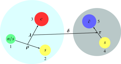
Figure 1: The Jacobi coordinates of the $\Xi_{c}^{(\prime,*)}\bar{D}_{s}^{*}/\Omega_{c}^{(*)}\bar{D}_{s}^{*}$-type hadronic molecular states. Here, $n$ stands for the up quark or the down quark, $s$ represents the strange quark, and $c$ denotes the charm quark.

As depicted in Fig. 1, the spatial wave functions of the hadronic molecular states are examined using the Jacobi coordinates ${\bf R}={{\bm{\rho}},{\bm{\lambda}},{\bm{\tau}},{\bm{\delta}}}$. These coordinates are employed to define the spatial distributions of the respective wave functions

$${\bm{\rho}} = {\bf r}_{2}-{\bf r}_{1},$$

$${\bm{\lambda}} = {\bf r}_{3}-\frac{m_{1}{\bf r}_{1}+m_{2}{\bf r}_{2}}{m_{1}+m_{2}},$$

$${\bm{\tau}} = {\bf r}_{5}-{\bf r}_{4},$$

$${\bm{\delta}} = \frac{m_{4}{\bf r}_{4}+m_{5}{\bf r}_{5}}{m_{4}+m_{5}}-\frac{m_{1}{\bf r}_{1}+m_{2}{\bf r}_{2}+m_{3}{\bf r}_{3}}{m_{1}+m_{2}+m_{3}},$$ (85)

and the spatial wave functions of the initial and final hadron states can be explicitly expressed as $\phi({\bm{\rho}})\phi({\bm{\lambda}})\phi({\bm{\tau}})\phi({\bm{\delta}})$. On the other hand, the coordinates of the quarks ${\bf r}_{j}~{}(j=1-5)$ can be written as

$${\bf r}_{j}=\sum\limits_{n}\alpha_{jn}{\bf R}_{n}=\alpha_{j1}{\bm{\rho}}+\alpha_{j2}{\bm{\lambda}}+\alpha_{j3}{\bm{\tau}}+\alpha_{j4}{\bm{\delta}}.$$ (86)

Thus, the ${\bf q}\cdot{\bf r}_{j}$ can be expanded by

$${\bf q}\cdot{\bf r}_{j}={\alpha}_{j1}{\bf q}\cdot{\bm{\rho}}+{\alpha}_{j2}{\bf q}\cdot{\bm{\lambda}}+{\alpha}_{j3}{\bf q}\cdot{\bm{\tau}}+{\alpha}_{j4}{\bf q}\cdot{\bm{\delta}}.$$ (87)

For the sake of convenience, we utilize a matrix representation to present the variable $\alpha$, which is defined as

$$\alpha=\left(\begin{array}[]{cccc}-\frac{m_{2}}{m_{1}+m_{2}}&-\frac{m_{3}}{m_{1}+m_{2}+m_{3}}&0&-\frac{m_{4}+m_{5}}{m_{1}+m_{2}+m_{3}+m_{4}+m_{5}}\\ \frac{m_{1}}{m_{1}+m_{2}}&-\frac{m_{3}}{m_{1}+m_{2}+m_{3}}&0&-\frac{m_{4}+m_{5}}{m_{1}+m_{2}+m_{3}+m_{4}+m_{5}}\\ 0&\frac{m_{1}+m_{2}}{m_{1}+m_{2}+m_{3}}&0&-\frac{m_{4}+m_{5}}{m_{1}+m_{2}+m_{3}+m_{4}+m_{5}}\\ 0&0&-\frac{m_{5}}{m_{4}+m_{5}}&\frac{m_{1}+m_{2}+m_{3}}{m_{1}+m_{2}+m_{3}+m_{4}+m_{5}}\\ 0&0&\frac{m_{4}}{m_{4}+m_{5}}&\frac{m_{1}+m_{2}+m_{3}}{m_{1}+m_{2}+m_{3}+m_{4}+m_{5}}\\ \end{array}\right).$$ (88)

To describe the spatial wave functions of the baryons and mesons, we take the simple harmonic oscillator (SHO) wave function, i.e.,

$$\phi_{n,l,m}(\beta,{\bf r}) = \sqrt{\frac{2n!}{\Gamma(n+l+\frac{3}{2})}}L_{n}^{l+\frac{1}{2}}(\beta^{2}r^{2})\beta^{l+\frac{3}{2}}$$ (89)

$$\times{\mathrm{e}}^{-\frac{\beta^{2}r^{2}}{2}}r^{l}Y_{lm}(\Omega),$$

where $Y_{lm}(\Omega)$ is the spherical harmonic function, $L_{n}^{l+\frac{1}{2}}(x)$ is the associated Laguerre polynomial, while $n$, $l$, and $m$ are the radial, orbital, and magnetic quantum numbers of the hadron, respectively. The parameter $\beta$ in Eq. (89) corresponds to the SHO wave function and has been approximately estimated to be around $0.4~{}{\rm GeV}$ in previous theoretical studies Liu:2011yp ; Li:2008xy . In this work, we adopt this value for consistency. However, it is worth noting that the transition magnetic moment and the radiative decay width may exhibit slight variations when scanning the $\beta$ value within the range of $0.3~{}{\rm GeV}$ to $0.5~{}{\rm GeV}$. For the hadronic molecular state, which represents a loosely bound system, the spatial wave function (the ${\bm{\delta}}$-degree of freedom in Fig. 1) significantly deviates from the SHO wave function. Hence, we derive the accurate spatial wave function for the molecular state by quantitatively solving the Schrödinger equation.

Furthermore, we employ the following equations Khersonskii:1988krb to expand the spatial wave function of the emitted photon, denoted as $e^{-i{\bf q}\cdot{\bf r}_{j}}$

$$e^{-i{\bf q}\cdot{\bf r}_{j}} = e^{-i\sum\limits_{n}\alpha_{jn}{\bf q}\cdot{\bf R}_{n}}=\prod\limits_{n}e^{-i\alpha_{jn}{\bf q}\cdot{\bf R}_{n}},$$ (90)

$$e^{-i\alpha_{jn}{\bf q}\cdot{\bf R}_{n}} = \sum\limits_{l=0}^{\infty}\sum\limits_{m=-l}^{l}4\pi(-i)^{l}j_{l}(\alpha_{jn}qR_{n})$$ (91)

$$\times Y_{lm}^{*}(\Omega_{\bf q})Y_{lm}(\Omega_{{\bf R}_{n}}).$$

Here, $j_{l}(x)$ is the spherical Bessel function. In the $S$-wave scheme, there only exists the $l=0$ part, which leads to the following relation

$$\langle\phi_{0,0,0}(\beta^{\prime},{\bf R}_{n})|e^{-i\alpha_{jn}{\bf q}\cdot{\bf R}_{n}}|\phi_{0,0,0}(\beta,{\bf R}_{n})\rangle$$

$$=\int\phi_{0,0,0}(\beta^{\prime},{\bf R}_{n})j_{0}(\alpha_{jn}qR_{n})\phi_{0,0,0}(\beta,{\bf R}_{n}){\rm d}^{3}{\bf R}_{n}$$

$$=\frac{2\sqrt{2}(\beta^{\prime}\beta)^{3/2}}{(\beta^{\prime 2}+\beta^{2})^{3/2}}e^{-\frac{\alpha_{jn}^{2}q^{2}}{2(\beta^{\prime 2}+\beta^{2})}}.$$ (92)

Based on the above discussion, we can perform a comprehensive analysis of the contributions from the spatial wave functions of the emitted photon, baryons, mesons, and hadronic molecules to the transition magnetic moment and the radiative decay width.

References

• (1) C. Amsler and N. A. Tornqvist, Mesons beyond the naive quark model, Phys. Rept. 389, 61-117 (2004).
• (2) E. S. Swanson, The New heavy mesons: A Status report, Phys. Rept. 429, 243-305 (2006).
• (3) S. Godfrey and S. L. Olsen, The Exotic $XYZ$ Charmonium-like Mesons, Ann. Rev. Nucl. Part. Sci. 58, 51-73 (2008).
• (4) N. Drenska, R. Faccini, F. Piccinini, A. Polosa, F. Renga and C. Sabelli, New Hadronic Spectroscopy, Riv. Nuovo Cim. 33, no.11, 633-712 (2010).
• (5) G. V. Pakhlova, P. N. Pakhlov and S. I. Eidelman, Exotic charmonium, Phys. Usp. 53, 219-241 (2010).
• (6) R. Faccini, A. Pilloni and A. D. Polosa, Exotic Heavy Quarkonium Spectroscopy: A Mini-review, Mod. Phys. Lett. A 27, 1230025 (2012).
• (7) X. Liu, An overview of $XYZ$ new particles, Chin. Sci. Bull.  59, 3815 (2014).
• (8) A. Hosaka, T. Iijima, K. Miyabayashi, Y. Sakai, and S. Yasui, Exotic hadrons with heavy flavors: $X$, $Y$, $Z$, and related states, Prog. Theor. Exp. Phys. 2016, 062C01 (2016).
• (9) H. X. Chen, W. Chen, X. Liu, and S. L. Zhu, The hidden-charm pentaquark and tetraquark states, Phys. Rep.  639, 1 (2016).
• (10) J. M. Richard, Exotic hadrons: review and perspectives, Few Body Syst. 57, 1185-1212 (2016).
• (11) R. F. Lebed, R. E. Mitchell and E. S. Swanson, Heavy-Quark QCD Exotica, Prog. Part. Nucl. Phys. 93 (2017), 143-194.
• (12) A. Ali, J. S. Lange and S. Stone, Exotics: Heavy Pentaquarks and Tetraquarks, Prog. Part. Nucl. Phys. 97, 123-198 (2017).
• (13) Y. Dong, A. Faessler and V. E. Lyubovitskij, Description of heavy exotic resonances as molecular states using phenomenological Lagrangians, Prog. Part. Nucl. Phys. 94, 282-310 (2017).
• (14) S. L. Olsen, T. Skwarnicki, and D. Zieminska, Nonstandard heavy mesons and baryons: Experimental evidence, Rev. Mod. Phys.  90, 015003 (2018).
• (15) F. K. Guo, C. Hanhart, U. G. Mei$\ss$ner, Q. Wang, Q. Zhao, and B. S. Zou, Hadronic molecules, Rev. Mod. Phys.  90, 015004 (2018).
• (16) C. Z. Yuan, The $XYZ$ states revisited, Int. J. Mod. Phys. A 33, no.21, 1830018 (2018).
• (17) Y. R. Liu, H. X. Chen, W. Chen, X. Liu, and S. L. Zhu, Pentaquark and tetraquark states, Prog. Part. Nucl. Phys.  107, 237 (2019).
• (18) R. M. Albuquerque, J. M. Dias, K. P. Khemchandani, A. Martínez Torres, F. S. Navarra, M. Nielsen and C. M. Zanetti, QCD sum rules approach to the $X,~{}Y$ and $Z$ states, J. Phys. G 46, no.9, 093002 (2019).
• (19) N. Brambilla, S. Eidelman, C. Hanhart, A. Nefediev, C. P. Shen, C. E. Thomas, A. Vairo, and C. Z. Yuan, The $XYZ$ states: Experimental and theoretical status and perspectives, Phys. Rep. 873, 1 (2020).
• (20) Y. Yamaguchi, A. Hosaka, S. Takeuchi and M. Takizawa, Heavy hadronic molecules with pion exchange and quark core couplings: a guide for practitioners, J. Phys. G 47, no.5, 053001 (2020).
• (21) L. Meng, B. Wang, G. J. Wang and S. L. Zhu, Chiral perturbation theory for heavy hadrons and chiral effective field theory for heavy hadronic molecules, Phys. Rept. 1019, 1-149 (2023).
• (22) H. X. Chen, W. Chen, X. Liu, Y. R. Liu and S. L. Zhu, An updated review of the new hadron states, Rept. Prog. Phys. 86, no.2, 026201 (2023).
• (23) R. Aaij et al. (LHCb Collaboration), Observation of $J/\psi$ Resonances Consistent with Pentaquark States in $\Lambda_{b}^{0}\rightarrow J/\psi K^{-}p$ Decays, Phys. Rev. Lett.  115, 072001 (2015).
• (24) R. Aaij et al. (LHCb Collaboration), Observation of a Narrow Pentaquark State, $P_{c}(4312)^{+}$, and of Two-Peak Structure of the $P_{c}(4450)^{+}$, Phys. Rev. Lett.  122, 222001 (2019).
• (25) J. J. Wu, R. Molina, E. Oset and B. S. Zou, Prediction of narrow $N^{*}$ and $\Lambda^{*}$ resonances with hidden charm above 4 GeV, Phys. Rev. Lett.  105, 232001 (2010).
• (26) W. L. Wang, F. Huang, Z. Y. Zhang, and B. S. Zou, $\Sigma_{c}\bar{D}$ and $\Lambda_{c}\bar{D}$ states in a chiral quark model, Phys. Rev. C 84, 015203 (2011).
• (27) Z. C. Yang, Z. F. Sun, J. He, X. Liu, and S. L. Zhu, The possible hidden-charm molecular baryons composed of anti-charmed meson and charmed baryon, Chin. Phys. C 36, 6 (2012).
• (28) J. J. Wu, T.-S. H. Lee, and B. S. Zou, Nucleon resonances with hidden charm in coupled-channel Models, Phys. Rev. C 85, 044002 (2012).
• (29) X. Q. Li and X. Liu, A possible global group structure for exotic states, Eur. Phys. J. C 74, 3198 (2014).
• (30) R. Chen, X. Liu, X. Q. Li, and S. L. Zhu, Identifying Exotic Hidden-Charm Pentaquarks, Phys. Rev. Lett.  115, 132002 (2015).
• (31) M. Karliner and J. L. Rosner, New Exotic Meson and Baryon Resonances from Doubly-Heavy Hadronic Molecules, Phys. Rev. Lett.  115, 122001 (2015).
• (32) R. Aaij et al. (LHCb Collaboration), Evidence of a $J/\psi\Lambda$ structure and observation of excited $\Xi^{-}$ states in the $\Xi^{-}_{b}\to J/\psi\Lambda K^{-}$ decay, Sci. Bull. 66, 1278-1287 (2021).
• (33) [LHCb], Observation of a $J/\psi\Lambda$ resonance consistent with a strange pentaquark candidate in $B^{-}\to J/\psi\Lambda\bar{p}$ decays, arXiv:2210.10346.
• (34) J. Hofmann and M. F. M. Lutz, Coupled-channel study of crypto-exotic baryons with charm, Nucl. Phys. A 763, 90 (2005).
• (35) J. J. Wu, R. Molina, E. Oset and B. S. Zou, Dynamically generated $N^{*}$ and $\Lambda^{*}$ resonances in the hidden charm sector around 4.3 GeV, Phys. Rev. C 84, 015202 (2011).
• (36) V. V. Anisovich, M. A. Matveev, J. Nyiri, A. V. Sarantsev, and A. N. Semenova, Nonstrange and strange pentaquarks with hidden charm, Int. J. Mod. Phys. A 30, 1550190 (2015).
• (37) Z. G. Wang, Analysis of the ${\frac{1}{2}}^{\pm}$ pentaquark states in the diquark-diquark-antiquark model with QCD sum rules, Eur. Phys. J. C 76, 142 (2016).
• (38) A. Feijoo, V. K. Magas, A. Ramos, and E. Oset, A hidden-charm $S=-1$ pentaquark from the decay of $\Lambda_{b}$ into $J/\psi\eta\Lambda$ states, Eur. Phys. J. C 76, no. 8, 446 (2016).
• (39) J. X. Lu, E. Wang, J. J. Xie, L. S. Geng, and E. Oset, The $\Lambda_{b}\rightarrow J/\psi K^{0}\Lambda$ reaction and a hidden-charm pentaquark state with strangeness, Phys. Rev. D 93, 094009 (2016).
• (40) H. X. Chen, L. S. Geng, W. H. Liang, E. Oset, E. Wang, and J. J. Xie, Looking for a hidden-charm pentaquark state with strangeness $S=-1$ from $\Xi^{-}_{b}$ decay into $J/\psi K^{-}\Lambda$, Phys. Rev. C 93, 065203 (2016).
• (41) R. Chen, J. He, and X. Liu, Possible strange hidden-charm pentaquarks from $\Sigma_{c}^{(*)}\bar{D}_{s}^{*}$ and $\Xi^{(^{\prime},*)}_{c}\bar{D}^{*}$ interactions, Chin. Phys. C 41, 103105 (2017).
• (42) X. Z. Weng, X. L. Chen, W. Z. Deng and S. L. Zhu, Hidden-charm pentaquarks and $P_{c}$ states, Phys. Rev. D 100, 016014 (2019).
• (43) C. W. Xiao, J. Nieves, and E. Oset, Prediction of hidden charm strange molecular baryon states with heavy quark spin symmetry, Phys. Lett. B 799, 135051 (2019).
• (44) C. W. Shen, H. J. Jing, F. K. Guo, and J. J. Wu, Exploring possible triangle singularities in the $\Xi^{-}_{b}\to K^{-}J/\psi\Lambda$ decay, Symmetry 12, 1611 (2020).
• (45) B. Wang, L. Meng, and S. L. Zhu, Spectrum of the strange hidden charm molecular pentaquarks in chiral effective field theory, Phys. Rev. D 101, 034018 (2020).
• (46) Q. Zhang, B. R. He, and J. L. Ping, Pentaquarks with the $qqs\bar{Q}Q$ configuration in the Chiral Quark Model, arXiv:2006.01042.
• (47) H. X. Chen, W. Chen, X. Liu, and X. H. Liu, Establishing the first hidden-charm pentaquark with strangeness, Eur. Phys. J. C 81, 409 (2021).
• (48) F. Z. Peng, M. J. Yan, M. Sánchez Sánchez, and M. P. Valderrama, The $P_{cs}(4459)$ pentaquark from a combined effective field theory and phenomenological perspectives, Eur. Phys. J. C 81, 666 (2021).
• (49) R. Chen, Can the newly reported $P_{cs}(4459)$ be a strange hidden-charm $\Xi_{c}\bar{D}^{*}$ molecular pentaquark?, Phys. Rev. D 103, 054007 (2021).
• (50) H. X. Chen, Hidden-charm pentaquark states through the current algebra: From their productions to decays, Chin. Phys. C 46, 093105 (2022).
• (51) M. Z. Liu, Y. W. Pan, and L. S. Geng, Can discovery of hidden charm strange pentaquark states help determine the spins of $P_{c}(4440)$ and $P_{c}(4457)$ ?, Phys. Rev. D 103, 034003 (2021).
• (52) C. W. Xiao, J. J. Wu and B. S. Zou, Molecular nature of $P_{cs}(4459)$ and its heavy quark spin partners, Phys. Rev. D 103, 054016 (2021).
• (53) M. L. Du, Z. H. Guo and J. A. Oller, Insights into the nature of the $P_{cs}(4459)$, Phys. Rev. D 104, 114034 (2021).
• (54) J. T. Zhu, L. Q. Song and J. He, $P_{cs}(4459)$ and other possible molecular states from $\Xi_{c}^{(*)}\bar{D}^{(*)}$ and $\Xi^{\prime}_{c}\bar{D}^{(*)}$ interactions, Phys. Rev. D 103, 074007 (2021).
• (55) X. K. Dong, F. K. Guo and B. S. Zou, A survey of heavy-antiheavy hadronic molecules, Progr. Phys. 41, 65-93 (2021).
• (56) K. Chen, R. Chen, L. Meng, B. Wang and S. L. Zhu, Systematics of the heavy flavor hadronic molecules, Eur. Phys. J. C 82, 581 (2022).
• (57) R. Chen and X. Liu, Mass behavior of hidden-charm open-strange pentaquarks inspired by the established $P_{c}$ molecular states, Phys. Rev. D 105, 014029 (2022).
• (58) K. Chen, B. Wang and S. L. Zhu, Heavy flavor molecular states with strangeness, Phys. Rev. D 105, 096004 (2022).
• (59) X. Hu and J. Ping, Investigation of hidden-charm pentaquarks with strangeness $S=-1$, Eur. Phys. J. C 82, 118 (2022).
• (60) X. W. Wang and Z. G. Wang, Analysis of $P_{cs}(4338)$ and related pentaquark molecular states via QCD sum rules*, Chin. Phys. C 47, no.1, 013109 (2023).
• (61) M. Karliner and J. R. Rosner, strange pentaquarks, Phys. Rev. D 106, 036024 (2022).
• (62) F. L. Wang and X. Liu, Emergence of molecular-type characteristic spectrum of hidden-charm pentaquark with strangeness embodied in the $P_{\psi s}^{\Lambda}(4338)$ and $P_{cs}(4459)$, Phys. Lett. B 835, 137583 (2022).
• (63) M. J. Yan, F. Z. Peng, M. Sánchez Sánchez and M. Pavon Valderrama, $P_{\psi s}^{\Lambda}(4338)$ pentaquark and its partners in the molecular picture, Phys. Rev. D 107, no.7, 074025 (2023).
• (64) L. Meng, B. Wang and S. L. Zhu, Double thresholds distort the line shapes of the $P_{\psi s}^{\Lambda}(4338)^{0}$ resonance, Phys. Rev. D 107, no.1, 014005 (2023).
• (65) K. Azizi, Y. Sarac and H. Sundu, Investigation of $P_{cs}(4459)^{0}$ pentaquark via its strong decay to $\Lambda J/\psi$, Phys. Rev. D 103, no.9, 094033 (2021).
• (66) R. Chen, Strong decays of the newly $P_{cs}(4459)$ as a strange hidden-charm $\Xi_{c}{\bar{D}}^{*}$ molecule, Eur. Phys. J. C 81, no.2, 122 (2021).
• (67) S. Clymton, H. J. Kim and H. C. Kim, Production of hidden-charm strange pentaquarks Pcs from the $K^{-}p\to J/\psi\Lambda$ reaction, Phys. Rev. D 104, no.1, 014023 (2021).
• (68) B. S. Zou, Building up the spectrum of pentaquark states as hadronic molecules, Sci. Bull. 66, 1258 (2021).
• (69) J. X. Lu, M. Z. Liu, R. X. Shi and L. S. Geng, Understanding $P_{cs}(4459)$ as a hadronic molecule in the $\Xi_{b}^{-}\to J/\psi\Lambda K^{-}$ decay, Phys. Rev. D 104, no.3, 034022 (2021).
• (70) J. Ferretti and E. Santopinto, The new $P_{\rm cs}(4459)$, $Z_{\rm cs}(3985)$, $Z_{\rm cs}(4000)$ and $Z_{\rm cs}(4220)$ and the possible emergence of flavor pentaquark octets and tetraquark nonets, Sci. Bull. 67, 1209 (2022).
• (71) E. Y. Paryev, Regarding the possibility to observe the LHCb hidden-charm strange pentaquark $P_{cs}(4459)^{0}$ in antikaon-induced $J/\psi$ meson production on protons and nuclei near the $J/\psi\Lambda$ production threshold, Nucl. Phys. A 1023, 122452 (2022).
• (72) S. X. Nakamura and J. J. Wu, Pole determination of $P_{\psi s}^{\Lambda}(4338)$ and possible $P_{\psi s}^{\Lambda}(4255)$ in $B^{-}\to J/\psi\Lambda\bar{p}$, Phys. Rev. D 108, no.1, L011501 (2023).
• (73) A. Giachino, A. Hosaka, E. Santopinto, S. Takeuchi, M. Takizawa and Y. Yamaguchi, Rich structure of the hidden-charm pentaquarks near threshold regions, arXiv:2209.10413.
• (74) J. A. Marsé-Valera, V. K. Magas and A. Ramos, Double-Strangeness Molecular-Type Pentaquarks from Coupled-Channel Dynamics, Phys. Rev. Lett. 130, no.9, 9 (2023).
• (75) P. G. Ortega, D. R. Entem and F. Fernandez, Strange hidden-charm $P_{\psi s}^{\Lambda}(4459)$ and $P_{\psi s}^{\Lambda}(4338)$ pentaquarks and additional $P_{\psi s}^{\Lambda}$, $P_{\psi s}^{\Sigma}$ and $P_{\psi ss}^{N}$ candidates in a quark model approach, Phys. Lett. B 838, 137747 (2023).
• (76) K. Chen, Z. Y. Lin and S. L. Zhu, Comparison between the $P_{\psi}^{N}$ and $P_{\psi s}^{\Lambda}$ systems, Phys. Rev. D 106, no.11, 116017 (2022).
• (77) J. T. Zhu, S. Y. Kong and J. He, $P^{\Lambda}_{\psi s}(4459)$ and $P^{\Lambda}_{\psi s}(4338)$ as molecular states in $J/\psi\Lambda$ invariant mass spectra, Phys. Rev. D 107, no.3, 034029 (2023).
• (78) Z. Y. Yang, F. Z. Peng, M. J. Yan, M. Sánchez Sánchez and M. Pavon Valderrama, Molecular $P_{\psi}$ pentaquarks from light-meson exchange saturation, arXiv:2211.08211.
• (79) H. Garcilazo and A. Valcarce, Hidden-flavor pentaquarks, Phys. Rev. D 106, no.11, 114012 (2022).
• (80) A. Feijoo, W. F. Wang, C. W. Xiao, J. J. Wu, E. Oset, J. Nieves and B. S. Zou, A new look at the $P_{cs}$ states from a molecular perspective, Phys. Lett. B 839, 137760 (2023).
• (81) F. L. Wang, R. Chen, and X. Liu, Prediction of hidden-charm pentaquarks with double strangeness, Phys. Rev. D 103, 034014 (2021).
• (82) F. L. Wang, X. D. Yang, R. Chen and X. Liu, Hidden-charm pentaquarks with triple strangeness due to the $\Omega_{c}^{(*)}\bar{D}_{s}^{(*)}$ interactions, Phys. Rev. D 103, 054025 (2021).
• (83) K. Azizi, Y. Sarac and H. Sundu, Investigation of hidden-charm double strange pentaquark candidate $P_{css}$ via its mass and strong decays, Eur. Phys. J. C 82, no.6, 543 (2022).
• (84) K. Azizi, Y. Sarac and H. Sundu, Investigation of a candidate spin-$\frac{1}{2}$ hidden-charm triple strange pentaquark state $P_{csss}$, Phys. Rev. D 107, no.1, 014023 (2023).
• (85) F. Schlumpf, Magnetic moments of the baryon decuplet in a relativistic quark model, Phys. Rev. D 48, 4478-4480 (1993).
• (86) S. Kumar, R. Dhir and R. C. Verma, Magnetic moments of charm baryons using effective mass and screened charge of quarks, J. Phys. G 31, 141-147 (2005).
• (87) G. Ramalho, K. Tsushima and F. Gross, A Relativistic quark model for the Omega-electromagnetic form factors, Phys. Rev. D 80, 033004 (2009).
• (88) R. L. Workman et al. [Particle Data Group], Review of Particle Physics, PTEP 2022 (2022), 083C01.
• (89) G. J. Wang, R. Chen, L. Ma, X. Liu and S. L. Zhu, Magnetic moments of the hidden-charm pentaquark states, Phys. Rev. D 94, 094018 (2016).
• (90) M. W. Li, Z. W. Liu, Z. F. Sun and R. Chen, Magnetic moments and transition magnetic moments of $P_{c}$ and $P_{cs}$ states, Phys. Rev. D 104, 054016 (2021).
• (91) F. Gao and H. S. Li, Magnetic moments of hidden-charm strange pentaquark states*, Chin. Phys. C 46, no.12, 123111 (2022).
• (92) F. L. Wang, H. Y. Zhou, Z. W. Liu and X. Liu, What can we learn from the electromagnetic properties of hidden-charm molecular pentaquarks with single strangeness?, Phys. Rev. D 106, 054020 (2022).
• (93) Y. R. Liu, P. Z. Huang, W. Z. Deng, X. L. Chen and S. L. Zhu, Pentaquark magnetic moments in different models, Phys. Rev. C 69, 035205 (2004).
• (94) P. Z. Huang, Y. R. Liu, W. Z. Deng, X. L. Chen and S. L. Zhu, Heavy pentaquarks, Phys. Rev. D 70, 034003 (2004).
• (95) S. L. Zhu, Pentaquarks, Int. J. Mod. Phys. A 19, 3439-3469 (2004).
• (96) A. R. Haghpayma, Magnetic Moment of the Pentaquark $\Theta^{+}$ State, arXiv:hep-ph/0609253.
• (97) C. Deng and S. L. Zhu, $T_{cc}^{+}$ and its partners, Phys. Rev. D 105, 054015 (2022).
• (98) H. Y. Zhou, F. L. Wang, Z. W. Liu and X. Liu, Probing the electromagnetic properties of the $\Sigma_{c}^{(*)}D^{(*)}$-type doubly charmed molecular pentaquarks, Phys. Rev. D 106, 034034 (2022).
• (99) F. Schlumpf, Relativistic constituent quark model of electroweak properties of baryons, Phys. Rev. D 47, 4114 (1993); erratum: Phys. Rev. D 49, 6246 (1994).
• (100) T. P. Cheng and L. F. Li, Why naive quark model can yield a good account of the baryon magnetic moments, Phys. Rev. Lett. 80, 2789-2792 (1998).
• (101) P. Ha and L. Durand, Baryon magnetic moments in a QCD based quark model with loop corrections, Phys. Rev. D 58, 093008 (1998).
• (102) R. Dhir and R. C. Verma, Magnetic Moments of ($J^{P}=3/2^{+}$) Heavy Baryons Using Effective Mass Scheme, Eur. Phys. J. A 42, 243-249 (2009).
• (103) A. Majethiya, B. Patel and P. C. Vinodkumar, Radiative decays of single heavy flavour baryons, Eur. Phys. J. A 42, 213-218 (2009).
• (104) N. Sharma, H. Dahiya, P. K. Chatley and M. Gupta, Spin $\frac{1}{2}^{+}$, spin $\frac{3}{2}^{+}$ and transition magnetic moments of low lying and charmed baryons, Phys. Rev. D 81, 073001 (2010).
• (105) N. Sharma, A. Martinez Torres, K. P. Khemchandani and H. Dahiya, Magnetic moments of the low-lying ${1/2}^{-}$ octet baryon resonances, Eur. Phys. J. A 49, 11 (2013).
• (106) R. Dhir, C. S. Kim and R. C. Verma, Magnetic Moments of Bottom Baryons: Effective mass and Screened Charge, Phys. Rev. D 88, 094002 (2013).
• (107) Z. Ghalenovi, A. A. Rajabi, S. x. Qin and D. H. Rischke, Ground-State Masses and Magnetic Moments of Heavy Baryons, Mod. Phys. Lett. A 29, 1450106 (2014).
• (108) A. Girdhar, H. Dahiya and M. Randhawa, Magnetic moments of $J^{P}=\frac{3}{2}^{+}$ decuplet baryons using effective quark masses in chiral constituent quark model, Phys. Rev. D 92, 033012 (2015).
• (109) A. Majethiya, K. Thakkar and P. C. Vinodkumar, Spectroscopy and decay properties of $\Sigma_{b},\Lambda_{b}$ baryons in quark-diquark model, Chin. J. Phys. 54, 495-502 (2016).
• (110) K. Thakkar, A. Majethiya and P. C. Vinodkumar, Magnetic moments of baryons containing all heavy quarks in the quark-diquark model, Eur. Phys. J. Plus 131, 339 (2016).
• (111) Z. Shah, K. Thakkar, A. K. Rai and P. C. Vinodkumar, Mass spectra and Regge trajectories of $\Lambda_{c}^{+}$, $\Sigma_{c}^{0}$, $\Xi_{c}^{0}$ and $\Omega_{c}^{0}$ baryons, Chin. Phys. C 40, 123102 (2016).
• (112) Z. Shah, K. Thakkar and A. K. Rai, Excited State Mass spectra of doubly heavy baryons $\Omega_{cc}$, $\Omega_{bb}$ and $\Omega_{bc}$, Eur. Phys. J. C 76, 530 (2016).
• (113) A. Kaur, P. Gupta and A. Upadhyay, Properties of $J^{P}=1/2^{+}$ baryon octets at low energy, PTEP 2017, 063B02 (2017).
• (114) Z. Shah and A. Kumar Rai, Spectroscopy of the $\Omega_{ccb}$ baryon in the hypercentral constituent quark model, Chin. Phys. C 42, 053101 (2018).
• (115) K. Gandhi, Z. Shah and A. K. Rai, Decay properties of singly charmed baryons, Eur. Phys. J. Plus 133, 512 (2018).
• (116) H. Dahiya, Transition magnetic moments of $J^{P}=\frac{3}{2}^{+}$ decuplet to $J^{P}=\frac{1}{2}^{+}$ octet baryons in the chiral constituent quark model, Chin. Phys. C 42, 093102 (2018).
• (117) V. Simonis, Improved predictions for magnetic moments and M1 decay widths of heavy hadrons, arXiv:1803.01809.
• (118) Z. Ghalenovi and M. Moazzen Sorkhi, Mass spectra and decay properties of $\Sigma_{{b}}$ and $\Lambda_{{b}}$ baryons in a quark model, Eur. Phys. J. Plus 133, 301 (2018).
• (119) K. Gandhi and A. K. Rai, Spectrum of strange singly charmed baryons in the constituent quark model, Eur. Phys. J. Plus 135, 213 (2020).
• (120) S. Rahmani, H. Hassanabadi and H. Sobhani, Mass and decay properties of double heavy baryons with a phenomenological potential model, Eur. Phys. J. C 80, 312 (2020).
• (121) A. Hazra, S. Rakshit and R. Dhir, Radiative M1 transitions of heavy baryons: Effective quark mass scheme, Phys. Rev. D 104, 053002 (2021).
• (122) C. Menapara and A. K. Rai, Spectroscopic investigation of light strange $S=-1$ $\Lambda$, $\Sigma$ and $S=-2$ $\Xi$ baryons, Chin. Phys. C 45, 063108 (2021).
• (123) C. Menapara and A. K. Rai, Spectroscopic Study of Strangeness$=-3$ $\Omega^{-}$ Baryon, Chin. Phys. C 46, 103102 (2022).
• (124) H. Mutuk, The status of $\Xi_{\mathrm{{cc}}}^{++}$ baryon: investigating quark-diquark model, Eur. Phys. J. Plus 137, 10 (2022).
• (125) C. Menapara and A. K. Rai, Spectroscopy of light baryons: $\Delta$ resonances, Int. J. Mod. Phys. A 37, no.27, 2250177 (2022).
• (126) L. Y. Glozman and D. O. Riska, The Charm and bottom hyperons and chiral dynamics, Nucl. Phys. A 603, 326-344 (1996); [erratum: Nucl. Phys. A 620, 510-510 (1997)].
• (127) W. X. Zhang, H. Xu and D. Jia, Masses and magnetic moments of hadrons with one and two open heavy quarks: Heavy baryons and tetraquarks, Phys. Rev. D 104, 114011 (2021).
• (128) T. M. Aliev, T. Barakat and M. Savci, Magnetic moments of heavy $J^{P}={1\over 2}^{+}$ baryons in light cone QCD sum rules, Phys. Rev. D 91, 116008 (2015).
• (129) B. Patel, A. K. Rai and P. C. Vinodkumar, Masses and magnetic moments of heavy flavour baryons in hyper central model, J. Phys. G 35, 065001 (2008).
• (130) T. M. Aliev, K. Azizi and A. Ozpineci, Radiative Decays of the Heavy Flavored Baryons in Light Cone QCD Sum Rules, Phys. Rev. D 79, 056005 (2009).
• (131) M. B. Wise, Chiral perturbation theory for hadrons containing a heavy quark, Phys. Rev. D 45, R2188 (1992).
• (132) R. Casalbuoni, A. Deandrea, N. Di Bartolomeo, R. Gatto, F. Feruglio, and G. Nardulli, Light vector resonances in the effective chiral Lagrangian for heavy mesons, Phys. Lett. B 292, 371 (1992).
• (133) R. Casalbuoni, A. Deandrea, N. Di Bartolomeo, R. Gatto, F. Feruglio, and G. Nardulli, Phenomenology of heavy meson chiral Lagrangians, Phys. Rep.  281, 145 (1997).
• (134) T. M. Yan, H. Y. Cheng, C. Y. Cheung, G. L. Lin, Y. C. Lin, and H. L. Yu, Heavy quark symmetry and chiral dynamics, Phys. Rev. D 46, 1148 (1992); [Phys. Rev. D 55, 5851E (1997)].
• (135) M. Bando, T. Kugo and K. Yamawaki, Nonlinear Realization and Hidden Local Symmetries, Phys. Rept.  164, 217 (1988).
• (136) M. Harada and K. Yamawaki, Hidden local symmetry at loop: A New perspective of composite gauge boson and chiral phase transition, Phys. Rept.  381, 1 (2003).
• (137) G. J. Ding, Are $Y(4260)$ and $Z_{2}^{+}$(4250) ${\rm D_{1}D}$ or ${\rm D_{0}D^{*}}$ hadronic molecules? Phys. Rev. D 79, 014001 (2009).
• (138) R. Chen, A. Hosaka, and X. Liu, Searching for possible $\Omega_{c}$-like molecular states from meson-baryon interaction, Phys. Rev. D 97, 036016 (2018).
• (139) R. Chen, Z. F. Sun, X. Liu, and S. L. Zhu, Strong LHCb evidence supporting the existence of the hidden-charm molecular pentaquarks, Phys. Rev. D 100, 011502 (2019).
• (140) J. Dey, V. Shevchenko, P. Volkovitsky and M. Dey, Radiative decays of $S$-wave charmed baryons, Phys. Lett. B 337, 185-188 (1994).
• (141) W. J. Deng, L. Y. Xiao, L. C. Gui and X. H. Zhong, Radiative transitions of charmonium states in a constituent quark model, arXiv:1510.08269.
• (142) W. J. Deng, H. Liu, L. C. Gui and X. H. Zhong, Charmonium spectrum and their electromagnetic transitions with higher multipole contributions, Phys. Rev. D 95, no.3, 034026 (2017).
• (143) W. J. Deng, H. Liu, L. C. Gui and X. H. Zhong, Spectrum and electromagnetic transitions of bottomonium, Phys. Rev. D 95, no.7, 074002 (2017).
• (144) V. K. Khersonskii, A. N. Moskalev and D. A. Varshalovich, Quantum Theory Of Angular Momentum, World Scientific Publishing Company, Singapore, 1988.
• (145) J. F. Liu and G. J. Ding, Bottomonium Spectrum with Coupled-Channel Effects, Eur. Phys. J. C 72, 1981 (2012).
• (146) D. M. Li and S. Zhou, On the nature of the $\pi_{2}(1880)$, Phys. Rev. D 79, 014014 (2009).