Hypernetwork approach to Bayesian MAML

Abstract

The main goal of Few-Shot learning algorithms is to enable learning from small amounts of data. One of the most popular and elegant Few-Shot learning approaches is Model-Agnostic Meta-Learning (MAML). The main idea behind this method is to learn the shared universal weights of a meta-model, which are then adapted for specific tasks. However, the method suffers from over-fitting and poorly quantifies uncertainty due to limited data size. Bayesian approaches could, in principle, alleviate these shortcomings by learning weight distributions in place of point-wise weights. Unfortunately, previous modifications of MAML are limited due to the simplicity of Gaussian posteriors, MAML-like gradient-based weight updates, or by the same structure enforced for universal and adapted weights.

In this paper, we propose a novel framework for Bayesian MAML called BayesianHMAML, which employs Hypernetworks for weight updates. It learns the universal weights point-wise, but a probabilistic structure is added when adapted for specific tasks. In such a framework, we can use simple Gaussian distributions or more complicated posteriors induced by Continuous Normalizing Flows.

1 Introduction

Few-Shot learning models easily adapt to previously unseen tasks based on a few labeled samples. One of the most popular and elegant among them is Model-Agnostic Meta-Learning (MAML) (Finn et al., 2017). The main idea behind this method is to produce universal weights which can be rapidly updated to solve new small tasks (see the first plot in Fig. 1). However, limited data sets lead to two main problems. First, the method tends to overfit to training data, preventing us from using deep architectures with large numbers of weights. Second, it lacks good quantification of uncertainty, e.g., the model does not know how reliable its predictions are. Both problems can be addressed by employing Bayesian Neural Networks (BNNs) (MacKay, 1992), which learn distributions in place of point-wise estimates.

There exist a few Bayesian modifications of the classical MAML algorithm. Bayesian MAML (Yoon et al., 2018), Amortized bayesian meta-learning (Ravi and Beatson, 2018), PACOH (Rothfuss et al., 2021, 2020), FO-MAML (Nichol et al., 2018), MLAP-M (Amit and Meir, 2018), Meta-Mixture (Jerfel et al., 2019) learn distributions for the common universal weights, which are then updated to per-task local weights distributions. The above modifications of MAML, similar to the original MAML, rely on gradient-based updates. Weights specialized for small tasks are obtained by taking a fixed number of gradient steps from the standard universal weights. Such a procedure needs two levels of Bayesian regularization and the universal distribution is usually employed as a prior for the per-task specializations (see the second plot in Fig. 1). However, the hierarchical structure complicates the optimization procedure and limits updates in the MAML procedure.

MAML     BayesianMAML     BayesianHMAML   BayesianHMAML

(Gaussian)       (CNF)

Figure 1: Comparison of four models: MAML (Finn et al., 2017), BayesianMAML (Yoon et al., 2018), as well as BayesianHMAML-G, and BayesianHMAML-CNF. In the classic MAML, we have universal weights $\theta$, which are adapted to $\theta^{\prime}_{i}$ for individual tasks $\mathcal{T}_{i}$. In BayesianMAML, the posterior distributions for individual small tasks are obtained in a few gradient-based updates from the universal distribution. In BayesianHMAML-G, we learn point-wise universal weights similar to MAML, but parameters of the specialized Gaussian posteriors are produced by a hypernetwork. Unlike BayesianMAML, the per-task distributions do not share a common prior distribution. In BayesianHMAML-CNF, the hypernetwork conditions a CNF, which can model arbitrary non-Gaussian posteriors.

The paper presents BayesianHMAML – a new framework for Bayesian Few-Shot learning. It simplifies the explained above weight-adapting procedure and thanks to the use of hypernetworks, enables learning more complicated posterior updates. Similar to the previous approaches, the final weight posteriors are obtained by updating from the universal weights. However, we avoid learning the aforementioned hierarchical structure by point-wise modeling of the universal weights. The probabilistic structure is added only later when specializing the model for a specific task. In BayesianHMAML updates from the universal weights to the per-task specialized ones are generated by hypernetworks instead of the previously used gradient-based optimization. Because hypernetworks can easily model more complex structures, they allow for better adaptations. In particular, we tested the standard Gaussian posteriors (see the third plot in Fig. 1) against more general posteriors induced by Continuous Normalizing Flows (CNF) (Grathwohl et al., 2018) (see the right-most plot in Fig. 1).

To the best of our knowledge, BayesianHMAML is the first approach that uses hypernetworks with Bayesian learning for Few-Shot learning tasks. Our contributions can be summarized as follows:

• We introduce a novel framework for Bayesian Few-Shot learning, which simplifies updating procedure and allows using complicated posterior distributions.

• Compared to the previous Bayesian modifications of MAML, BayesianHMAML employs the hypernetworks architecture for producing significantly more flexible weight updates.

• We implement two versions of the model: BayesianHMAML-G, a classical Gaussian posterior and a generalized BayesianHMAML-CNF, relying on Conditional Normalizing Flows.

2 Background

This section introduces all the notions necessary for understanding our method. We start by presenting the background and notation for Few-Shot learning. Then, we describe how the MAML algorithm works and introduce the general idea of Hypernetworks dedicated to MAML updates. Finally, we briefly explain Conditional Normalizing Flows.

The terminology

describing the Few-Shot learning setup is dispersive due to the colliding definitions used in the literature. Here, we use the nomenclature derived from the Meta-Learning literature, which is the most prevalent at the time of writing (Wang et al., 2020; Sendera et al., 2022).

Let $\mathcal{S}=\{(\mathbf{x}_{l},\mathbf{y}_{l})\}_{l=1}^{L}$ be a support-set containing $L$ input-output pairs with classes distributed uniformly. In the One-Shot scenario, each class is represented by a single example, and $L=K$, where $K$ is the number of the considered classes in the given task. In the Few-Shot scenarios, each class usually has from $2$ to $5$ representatives in the support set $\mathcal{S}$.

Let $\mathcal{Q}=\{(\mathbf{x}_{m},\mathbf{y}_{m})\}_{m=1}^{M}$ be a query set (sometimes referred to in the literature as a target set), with examples of $M$, where $M$ is typically an order of magnitude greater than $K$. Support and query sets are grouped in task $\mathcal{T}=\{\mathcal{S},\mathcal{Q}\}$. Few-Shot models have randomly selected examples from the training set $\mathcal{D}=\{\mathcal{T}_{n}\}^{N}_{n=1}$ during training. During inference, we consider task $\mathcal{T}_{*}=\{\mathcal{S}_{*},\mathcal{X}_{*}\}$, where $\mathcal{S}_{*}$ is a set of support with known classes and $\mathcal{X}_{*}$ is a set of unlabeled query inputs. The goal is to predict the class labels for the query inputs $\mathbf{x}\in\mathcal{X}_{*}$, assuming support set $\mathcal{S}_{*}$ and using the model trained on the data $\mathcal{D}$.

Model-Agnostic Meta-Learning (MAML)

MAML (Finn et al., 2017) is one of the standard algorithms for Few-Shot learning, which learns the parameters of a model so that it can adapt to a new task in a few gradient steps. For the model, we use a neural network $f_{\theta}$ parameterized by weights $\theta$. Its architecture consists of a feature extractor (backbone) $E(\cdot)$ and a fully connected layer. The universal weights $\theta=(\theta^{E},\theta^{H})$ include $\theta^{E}$ for the feature extractor and $\theta^{H}$ for the classification head.

When adapting for a new task $\mathcal{T}_{i}=\{\mathcal{S}_{i},\mathcal{Q}_{i}\}$, the parameters $\theta$ are updated to $\theta^{\prime}_{i}$. Such an update is achieved in one or more gradient descent updates on $\mathcal{T}_{i}$. In the simplest case of one gradient update, the parameters are updated as follows:

$$\theta^{\prime}_{i}=\theta-\alpha\nabla_{\theta}\mathcal{L}_{\mathcal{T}_{i}}(f_{\theta}),$$

where $\alpha$ is a step size hyperparameter. The loss function for a data set $\mathcal{D}$ is cross-entropy. The meta-optimization across tasks is performed via stochastic gradient descent (SGD):

$$\theta\leftarrow\theta-\beta\nabla_{\theta}\sum_{\mathcal{T}_{i}\sim p(T)}\mathcal{L}_{\mathcal{T}_{i}}(f_{\theta^{\prime}_{i}})$$

where $\beta$ is the meta step size (see Fig. 1).

Hypernetwork approche to MAML.

HyperMAML (Przewięźlikowski et al., 2022) is a generalization of the MAML algorithm, which uses non-gradient-based updates generated by hypernetworks (Ha et al., 2016). Analogically to MAML, it considers a model represented by a function $f_{\theta}$ with parameters $\theta$. When adapting to a new task $\mathcal{T}_{i}$, the parameters of the model $\theta$ become $\theta^{\prime}_{i}$. Contrary to MAML, in HyperMAML the updated parameters $\theta^{\prime}_{i}$ are computed using a hypernetwork $H_{\phi}$ as

$$\theta^{\prime}_{i}=\theta+H_{\phi}(S_{i},\theta).$$

The hypernetwork $H_{\phi}$ is a neural network consisting of a feature extractor $E(\cdot)$, which transforms support sets into a lower-dimensional representation, and fully connected layers aggregate the representation. To achieve permutation invariance, the embeddings are sorted according to their respective classes before aggregation.

Similarly to MAML, the universal weights $\theta$ consist of the features extractor’s weights $\theta_{E}$ and the classification head’s weights $\theta_{H}$, i.e., $\theta=(\theta_{E},\theta_{H})$. However, HyperMAML keeps $\theta_{E}$ shared between tasks and updates only $\theta_{H}$, e.g.,

$$\theta^{\prime}_{i}=(\theta^{\prime E}_{i},\theta^{\prime H}_{i})=(\theta^{E}_{i},\theta^{H}_{i}+H_{\phi}(S_{i},\theta)).$$

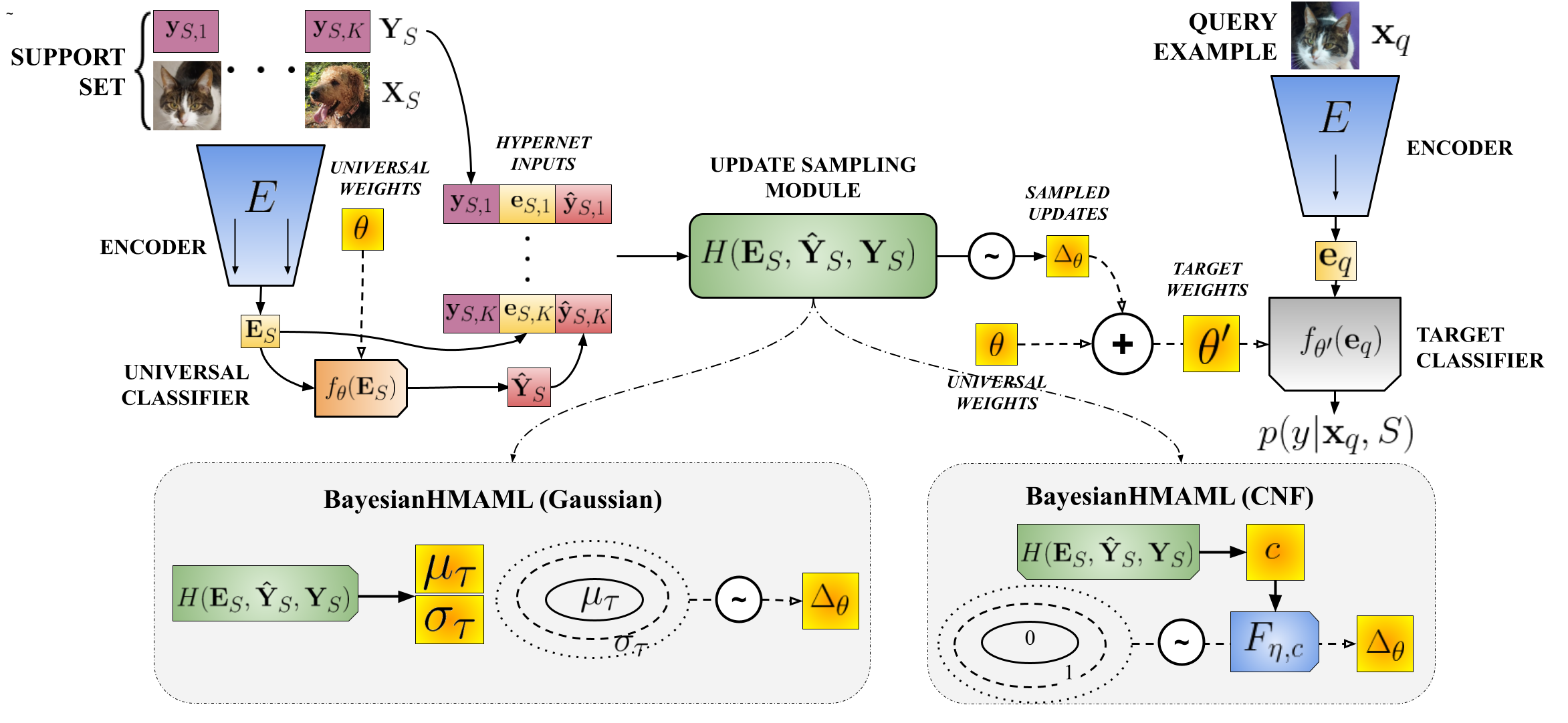
Figure 2: BayesianHMAML: Instead of updating the classifier weights with gradient descent, we use a hypernetwork $H$ to aggregate information from the support set $\mathcal{S}$ and to produce posterior parameters. First, the support set is transformed by an encoder. The embedded symbols $\mathbf{E}_{\mathcal{S}}$ are then concatenated with the original labels and predictions given by the universal weights. This representation is passed to a hypernetwork $H(\mathbf{E}_{\mathcal{S}},\mathbf{\hat{Y}}_{\mathcal{S}},\mathbf{Y}_{\mathcal{S}})$ to produce posterior distributions. In our work, we consider two posterior variants: Gaussian and CNF-based. Using the hypernetwork for weight updates $\theta$ allows for larger and smarter adaptations of the posterior parameters. In the end, we sample weight updates $\Delta\theta$ from the posterior distribution to obtain weights $\theta^{\prime}=\theta+\Delta\theta$ dedicated to a specific task.

Continuous Normalizing Flows (CNF).

The idea of normalizing flows (Dinh et al., 2014) relies on the transformation of a simple prior probability distribution $P_{Z}$ (usually a Gaussian one) defined in the latent space $Z$ into a complex one in the output space $Y$ through a series of invertible mappings: $F_{\eta}=F_{K}\circ\ldots\circ F_{1}:Z\to Y.$ The log-probability density of the output variable is given by the change of variables formula

$$\log P_{Y}(y;\eta)=\log P_{Z}(z)-\sum_{k=1}^{K}\log\left|\det\frac{\partial F_{k}}{\partial z_{k-1}}\right|,$$

where $z=F_{\eta}^{-1}(y)$ and $P(y;\eta)$ denotes the probability density function induced by the normalizing flow with parameters $\eta$. The intermediate layers $F_{i}$ must be designed so that both the inverse map and the determinant of the Jacobian are computable.

The continuous normalizing flow (Chen et al., 2018) is a modification of the above approach, where instead of a discrete sequence of iterations, we allow the transformation to be defined by a solution to a differential equation $\frac{\partial z(t)}{\partial t}=g(z(t),t),$ where $g$ is a neural network that has an unrestricted architecture. CNF, $F_{\eta}:Z\to Y$, is a solution of differential equations with the initial value problem $z(t_{0})=y$, $\frac{\partial z(t)}{\partial t}=g_{\eta}(z(t),t)$. In such a case, we have

$$\begin{array}[]{c}F_{\eta}(z)=F_{\eta}(z(t_{0}))=z(t_{0})+\int^{t_{1}}_{t_{0}}g_{\eta}(z(t),t)dt,\\[10.00002pt] F_{\eta}^{-1}(y)=y+\int_{t_{1}}^{t_{0}}g_{\eta}(z(t),t)dt,\end{array}$$

where $g_{\eta}$ defines the continuous-time dynamics of the flow $F_{\eta}$ and $z(t_{1})=y$.

The logarithmic probability of $y\in Y$ can be calculated by:

$$\log P_{Y}(y;\theta)=\log P_{Z}(F_{\theta}^{-1}(y))-\int^{t_{1}}_{t_{0}}\mathrm{Tr}\left(\frac{\partial g_{\theta}}{\partial z(t)}\right)dt.$$

The main advantage of normalizing flows (both discrete and continuous ones) is that they are not restricted to any predefined class of distributions, e.g. Gaussian densities. For example, flow models can reliably describe densities of high-dimensional image data (Kingma and Dhariwal, 2018).

3 BayesianHMAML – a new framework for Bayesian learning

In this section, we present BayesianHMAML – a Bayesian extension of the classical MAML. The most straightforward Bayesian treatment for such a model is to pose priors for the model parameters and learn their posteriors. In particular, for MAML one needs to learn posterior distributions for both $\theta$ and $\theta^{\prime}$. This naturally hints towards a hierarchical Bayesian model: $\theta\rightarrow\theta^{\prime}_{i}\rightarrow\mathcal{T}_{i}$, which was previously proposed in (Ravi and Beatson, 2018; Chen and Chen, 2022). Hence, variational inference along with reparametrization gradients (i.e. Bayes by backpropagation (Blundell et al., 2015)) is typically used, and the following objective (evidence lower bound) is maximized with respect to variational parameters $\lambda_{i}$ and $\psi$:

$$\begin{array}[]{c}\mathcal{L}_{\mathcal{D}}=\\[10.00002pt] \mathbb{E}_{q(\theta|\psi)}\!\!\underbrace{\left[\sum_{i}^{N}\mathbb{E}_{q(\theta^{\prime}_{i}|\lambda_{i})}\left[\log p(\mathcal{T}_{i}|\theta^{\prime}_{i})-\textit{KL}\left(q(\theta^{\prime}_{i}|\lambda_{i})\|p(\theta^{\prime}_{i}|\theta)\right)\right]\right]}_{\mathcal{L}_{\mathcal{T}_{i}}}-\textit{KL}(q(\theta|\psi)\|p(\theta))\end{array}$$

where $q(\theta^{\prime}_{i}|\lambda_{i})$ and $q(\theta|\psi)$ are respectively per-task posterior approximation and approximate posterior for the universal weights. They are tied together by the prior $p(\theta^{\prime}_{i}|\theta)$.

The above formulation poses some challenges. First of all, updates are limited by the posterior of universal weights. Furthermore, the same distribution is used for the posterior weights for universal and updated weights. Finally, the Gaussian distribution is used for both posteriors.

Learned objective.

We propose an alternative approach that alleviates the problems of previous attempts at Bayesian MAML. Contrary to them, we do not learn distributions for universal parameters $\theta$, but instead learn them in a pointwise manner. Distributional posteriors we learn only for individual task-specialized $\theta^{\prime}_{i}$, where we assume their independence. Furthermore, we remove the coupling prior between $\theta$ and $\theta^{\prime}_{i}$, and finally, we propose a basic non-hierarchical prior $p(\theta^{\prime}_{i})$ instead.

BayesianHMAML’s learning objective takes the following form:

$$\begin{array}[]{c}\mathcal{L}^{our}_{D}=\sum_{i}^{N}\mathbb{E}_{q(\theta^{\prime}_{i}|\lambda_{i}(\theta,\mathcal{S}_{i}))}\big{[}\log p(\mathcal{T}_{i}|\theta^{\prime}_{i})-\gamma\cdot\textit{KL}\left(q(\theta^{\prime}_{i}|\theta,\lambda_{i}(\theta,\mathcal{S}_{i}))\|p(\theta^{\prime}_{i})\right)\big{]},\end{array}$$

where we used the standard normal priors for the weights of the neural network $f$, i.e., $p(\theta^{\prime}_{i})=\mathcal{N}(\theta^{\prime}_{i}|0,\mathbb{I})$. The hyperparameter $\gamma$ allows controlling the impact of the priors and compensating for model misspecification. Overall, the proposed modifications enable better optima for the objective and simplify the optimization landscape helping convergence.

Treatment of parameters.

BayesianHMAML is a generalization of HyperMAML. Here however the weight updates result in posterior distributions instead of point-wise weights. In particular, when adapting a function $f_{\theta}$ with parameters $\theta$ to a task $\mathcal{T}_{i}$ the updated model’s parameters

$$\theta^{\prime}_{i}\sim q(\theta|\lambda_{i}(\theta,S_{i})).$$

In BayesianHMAML the parameters $\lambda_{i}$ are modeled by a hypernetwork as

$$\lambda_{i}(\theta,S_{i}):=H_{\phi}(\theta,S_{i}).$$

The hypernetwork $H_{\phi}$ takes support set $S_{i}$ and universal weights $\theta$ and when combined with the universal weights $\theta$ produces the posterior distribution $q$. Thanks to the hypernetwork, we obtain unconstrained updates and can model arbitrary posterior distributions, potentially improving over all previous non-hypernetwork models. Furthermore, the hypernetwork $H$ has a fixed number of parameters, regardless of how many tasks $\mathcal{T}_{i}$ are used for training. The amortized learning scheme has twofold benefits: (1) faster training; (2) regularization of learned parameters through shared architecture and common weights $\phi$.

We implemented two variants of BayesianHMAML: one using the standard Gaussian posterior and a generalized one with a flow-based posterior distribution.

Gaussian version.

BayesianHMAML-G is a simple realization of BayesianHMAML. In this approach, the hypernetwork $H_{\phi}$ returns the mean update and covariance matrix of a Gaussian posterior:

$$(\mu_{\theta}(\mathcal{S}_{i}),\sigma_{\theta}(\mathcal{S}_{i})):=H_{\phi}(\mathcal{S}_{i},\theta).$$

Weights are then sampled from the induced posterior:

$$\theta^{\prime}_{i}\sim\mathcal{N}(\theta+\mu_{\theta}(\mathcal{S}_{i}),\sigma_{\theta}(\mathcal{S}_{i})),$$

We apply here the mean-field assumption, but note the standard deviations $\sigma$ are not entirely independent. Due to the used amortization scheme, they are tied together and to the means $\mu$ by shared weights $\phi$ of the hypernetwork. Posterior means however are additionally explicitly dependent by the universal weights $\theta$. Like the classic MAML, any change of $\theta$ affects all the values of $\theta^{\prime}_{i}$.

CNF version.

BayesianHMAML-CNF is a generalization of BayesianHMAML-G, where we use conditional flows to produce weight posteriors for the specialized tasks. Similar to BayesianHMAML-G, we employ a hypernetwork to amortize updates of the target model parameters. However, in the above model the hypernetwork outputs parameters of a Gaussian distribution, whereas in BayesianHMAML-CNF it is responsible for conditioning a flow $F_{\eta,C(\theta,\mathcal{S}_{i})}(\cdot)$(see Fig. 2 for comparison):

$$C(\theta,\mathcal{S}_{i}):=H_{\phi}(\mathcal{S}_{i},\theta),$$

The conditioning vector $C$ is added to each layer of the flow to parameterize function $g_{\theta,C}$, so in the end, the flow $F_{\eta,C}$ depends on trainable parameters $\eta$ and conditioning parameters $C$. Then, the posterior for a task $\mathcal{T}_{i}$ is obtained by a two-stage process:

$$\Delta\theta^{\prime}_{i}\sim F_{\eta,C(\theta,\mathcal{S}_{i})}$$

$$\theta^{\prime}_{i}=\theta+\Delta\theta^{\prime}_{i},$$

where the shape of the posterior distribution is determined by the flow $F$, but its position, similarly to BayesianHMAML-G, mainly by the universal weights. From the implementation point of view, sampling from the conditioned flow also happens in two stages. First, we sample some $z$ from a flow prior and then, push this $z$ through a chain of deterministic transformations to obtain the final sample. Formally,

$$\Delta\theta^{\prime}_{i}:=F_{\eta,C(\theta,\mathcal{S}_{i})}(z),\mbox{ where }z\sim\mathrm{N}(0,t\cdot\mathbb{I}),$$

where $t$ is a hyperparameter, we used $t=0.1$.

Architecture of BayesianHMAML.

The goal here is to predict the class distribution $p(\mathbf{y}|{x}_{q},\mathcal{S})$, given a single query example $\mathbf{x}_{q}$, and a set of support examples $\mathcal{S}$. The architecture of BayesianHMAML is illustrated in Fig. 2. Following MAML, we consider a parametric function $f_{\theta}$, which models the discriminative distribution for the classes. In addition, our architecture consists of a trainable encoding network $E(\cdot)$, which transforms data into a low-dimensional representation. The predictions are then calculated following

$$p(\mathbf{y}|{x}_{q},\theta^{\prime})=f_{\theta^{\prime}}(\mathbf{e}_{q}),$$

where $\mathbf{e}_{q}$ is the query example $\mathbf{x}_{q}$ transformed using encoder $E(\cdot)$, and $\theta^{\prime}$ come from the posterior distribution for a considered task (either in BayesianHMAML-G or BayesianHMAML-CNF variant). In contrast to the MAML gradient-based adaptations, we predict weights directly from the support set using a hypernetwork. The hypernetwork observes support examples with the corresponding true labels and decides how the global parameters $\theta$ should be adjusted for a considered task. The two possible variants: BayesianHMAML-G and BayesianHMAML-CNF are illustrated (denoted by gray squares) in Fig. 2.

In BayesianHMAML, parameters of the learned posterior distribution are obtained by the hypernetwork $H_{\phi}(\theta,\mathcal{S})$. First, each of the inputs from support set $\mathcal{S}$ is transformed by Encoder $E(\cdot)$ to obtain low-dimensional matrix of embeddings $\mathbf{E}_{\mathcal{S}}=[\mathbf{e}_{\mathcal{S},1},\dots,\mathbf{e}_{\mathcal{S},K}]^{\mathrm{T}}.$ Next, the corresponding class labels for support examples, $\mathbf{Y}_{\mathcal{S}}=[\mathbf{y}_{\mathcal{S},1},\dots,\mathbf{y}_{\mathcal{S},K}]^{\mathrm{T}}$ are concatenated to the corresponding embeddings stored in the matrix $\mathbf{E}_{\mathcal{S}}$. Furthermore, we calculate the predicted values for the examples in the support set using the general model as $f_{\theta}(\mathbf{E}_{\mathcal{S}})=\mathbf{\hat{Y}_{\mathcal{S}}},$ and also concatenate them into $\mathbf{E}_{\mathcal{S}}$. The predictions of the global model $f_{\theta}$ help identify classification errors and correct them by weight adaptation.

Finally, the transformed support $\mathbf{E}_{\mathcal{S}}$, together with true labels $\mathbf{Y}_{\mathcal{S}}$, and the corresponding predictions $\mathbf{\hat{Y}_{\mathcal{S}}}$ from the model with universal weights are passed as input to the hypernetwork as $H(\mathbf{E}_{\mathcal{S}},\mathbf{\hat{Y}}_{\mathcal{S}},\mathbf{Y}_{\mathcal{S}})$, which then predicts the posterior controlling parameters. In our case, the hypernetwork consists of fully-connected layers with ReLU activations.

Implementation details.

Practical learning of BayesianHMAML is performed with stochastic gradients calculated w.r.t to the universal weights $\theta$ (i.e., $\nabla_{\theta}\mathcal{L}^{our}_{\mathcal{T}}$), the hypernetwork weights $\phi$ (i.e., $\nabla_{\phi}\mathcal{L}^{our}_{\mathcal{T}}$), and in case of BayesianHMAML-CNF also w.r.t $\eta$ (i.e., $\nabla_{\eta}\mathcal{L}^{our}_{\mathcal{T}}$), all of which have fixed sizes, which do not depend on the number of tasks $N$. We approximate the learning objective using mini-batches as

$$\begin{array}[]{cc}\mathcal{L}^{our}_{\mathcal{T}}=\sum\limits_{\mathcal{T}_{i}\sim p(\mathcal{T})}\Big{[}\frac{1}{P}\sum_{\theta^{\prime}_{i}\sim q(\theta,\lambda_{i}(\theta,\mathcal{S}_{i}))}\big{[}\mathcal{L}_{\mathcal{T}_{i}}(f_{\theta_{i}^{\prime}})-\gamma\textit{KL}(q(\theta_{i}^{\prime}|\theta,\lambda_{i}(\theta,\mathcal{S}_{i}))\|\mathcal{N}(\theta_{i}^{\prime}|0,\mathbb{I}))\big{]}\Big{]},\end{array}$$

where in each iteration we sample some number of tasks from $p(\mathcal{T})$ and then, for each task, we sample $P=5$ samples $\theta^{\prime}_{i}$ from the posterior $q$. How exactly is the sampling (and reparametrization) performed, depends on whether we use BayesianHMAML-G or BayesianHMAML-CNF.

For BayesianHMAML-G the KL-divergence can be calculated in a closed form. For BayesianHMAML-CNF we use a Monte-Carlo estimate of $P$ samples:

$$\begin{array}[]{cc}\textit{KL}(\cdot)=\frac{1}{P}\sum_{z\sim\mathcal{N}(0,t\cdot\mathbb{I})}\big{(}\log\mathcal{N}\left(F^{-1}_{\eta,C}(\Delta\theta^{\prime}_{i}|0,t\cdot\mathbb{I}\right)+\log\det|J|-\log N(\theta^{\prime}_{i}|0,\mathbb{I})\big{)},\end{array}$$

where $\Delta\theta^{\prime}_{i}\equiv F_{\eta,C}(z)$ and $J$ is the flow transition Jacobian. Contrary to non-amortized methods, BayesianHMAML is easy to maintain (and scales well) since we need to store only a fixed number of parameters $\{\theta,\psi\}$ (or in case of BayesianHMAML-CNF: $\{\theta,\psi,\eta\}$). Finally, for the hyperparameter $\gamma$, we apply an annealing scheme (Bowman et al., 2016): the parameter $\gamma$ grows from zero to a fixed constant during training. The final value $\gamma_{max}$ is a hyperparameter of the model.

4 Related Work

The problem of Meta-Learning and Few-Shot learning (Hospedales et al., 2020; Schmidhuber, 1992; Bengio et al., 1992) is currently one of the most important topics in deep learning, with the abundance of methods emerging as a result. They can be roughly categorized into three groups: Model-based methods, Metric-based methods, Optimization-based methods. In all these groups, we can find methods that use Hypernetworks and Bayesian learning (but not both at the same time). We briefly review the approaches below.

Model-based methods aim to adapt to novel tasks quickly by utilizing mechanisms such as memory (Ravi and Larochelle, 2017; Mishra et al., 2018; Zhen et al., 2020), Gaussian Processes (Rasmussen, 2003; Patacchiola et al., 2020; Wang et al., 2021; Sendera et al., 2021), or generating fast weights based on the support set with set-to-set architectures (Qiao et al., 2017; Bauer et al., 2017; Ye et al., 2018; Zhmoginov et al., 2022). Other approaches maintain a set of weight templates and, based on those, generate target weights quickly through gradient-based optimization such as (Zhao et al., 2020). The fast weights approaches can be interpreted as using Hypernetworks (Ha et al., 2016) – models which learn to generate the parameters of neural networks performing the designated tasks.

Metric-based methods learn a transformation to a feature space where the distance between examples from the same class is small. The earliest examples of such methods are Matching Networks (Vinyals et al., 2016) and Prototypical Networks (Snell et al., 2017). Subsequent works show that metric-based approaches can be improved by techniques such as learnable metric functions (Sung et al., 2018), conditioning the model on tasks (Oreshkin et al., 2018) or predicting the parameters of the kernel function to be calculated between support and query data with Hypernetworks (Sendera et al., 2022). In (Rusu et al., 2018), authors introduce a meta-learning technique that uses a generative parameter model to capture the diverse range of parameters useful for distribution over tasks.

Table 1: Classification accuracy for inference on ${CUB}$ and ${mini-ImageNet}$ data sets in the $1$-shot and $5$-shot settings. The highest results are in bold and the second-highest in italic.

	CUB		mini-ImageNet
Method	1-shot	5-shot	1-shot	5-shot
Feature Transfer (Zhuang et al., 2020)	$46.19\pm 0.64$	$68.40\pm 0.79$	$39.51\pm 0.23$	$60.51\pm 0.55$
ProtoNet (Snell et al., 2017)	$52.52\pm 1.90$	$75.93\pm 0.46$	$44.19\pm 1.30$	$64.07\pm 0.65$
MAML (Finn et al., 2017)	$56.11\pm 0.69$	$74.84\pm 0.62$	$45.39\pm 0.49$	$61.58\pm 0.53$
MAML++ (Antoniou et al., 2018)	–	–	$52.15\pm 0.26$	$\mathit{68.32\pm 0.44}$
FEAT (Ye et al., 2018)	$\mathbf{68.87\pm 0.22}$	$\mathbf{82.90\pm 0.15}$	$\mathbf{55.15\pm 0.20}$	$\mathbf{71.61\pm 0.16}$
LLAMA (Grant et al., 2018)	–	–	$49.40\pm 1.83$	–
VERSA (Gordon et al., 2018)	–	–	$48.53\pm 1.84$	$67.37\pm 0.86$
Amortized VI (Gordon et al., 2018)	–	–	$44.13\pm 1.78$	$55.68\pm 0.91$
DKT + BNCosSim (Patacchiola et al., 2020)	$62.96\pm 0.62$	$77.76\pm 0.62$	$49.73\pm 0.07$	$64.00\pm 0.09$
VAMPIRE (Nguyen et al., 2020)	–	–	$51.54\pm 0.74$	$64.31\pm 0.74$
ABML (Ravi and Beatson, 2018)	$49.57\pm 0.42$	$68.94\pm 0.16$	$45.00\pm 0.60$	–
OVE PG GP + Cosine (ML) (Snell and Zemel, 2020)	$63.98\pm 0.43$	$77.44\pm 0.18$	$50.02\pm 0.35$	$64.58\pm 0.31$
OVE PG GP + Cosine (PL) (Snell and Zemel, 2020)	$60.11\pm 0.26$	$79.07\pm 0.05$	$48.00\pm 0.24$	$67.14\pm 0.23$
Bayesian MAML (Yoon et al., 2018)	$55.93\pm 0.71$	–	$\mathit{53.80\pm 1.46}$	$64.23\pm 0.69$
HyperMAML (Przewięźlikowski et al., 2022)	$66.11\pm 0.28$	$78.89\pm 0.19$	$51.84\pm 0.57$	$66.29\pm 0.43$
BayesianHMAML (G)	$66.57\pm 0.47$	$79.86\pm 0.31$	$52.54\pm 0.46$	$67.39\pm 0.35$
BayesianHMAML (G)+adapt.	$\mathit{66.92\pm 0.38}$	$\mathit{80.47\pm 0.38}$	$52.69\pm 0.38$	$68.24\pm 0.47$
BayesianHMAML (CNF)	$61.55\pm 0.69$	$75.41\pm 0.21$	$49.39\pm 0.33$	$64.77\pm 0.21$
BayesianHMAML (CNF)+adapt.	$62.15\pm 0.51$	$75.69\pm 0.32$	$49.61\pm 0.24$	$65.48\pm 0.43$

Optimization-based methods such as MetaOptNet (Lee et al., 2019) is based on the idea of an optimization process over the support set within the Meta-Learning framework. Arguably, the most popular of this family of methods is Model-Agnostic Meta-Learning (MAML) (Finn et al., 2017). In literature, we have various techniques for stabilizing its training and improving performance, such as Multi-Step Loss Optimization (Antoniou et al., 2018), or using the Bayesian variant of MAML (Yoon et al., 2018).

Due to a need for calculating second-order derivatives when computing the gradient of the meta-training loss, training the classical MAML introduces a significant computational overhead. The authors show that in practice, the second-order derivatives can be omitted at the cost of small gradient estimation error and minimally reduced accuracy of the model (Finn et al., 2017; Nichol et al., 2018). Methods such as iMAML and Sign-MAML propose to solve this issue with implicit gradients or Sign-SGD optimization (Rajeswaran et al., 2019; Fan et al., 2021). The optimization process can also be improved by training the base initialization (Munkhdalai and Yu, 2017; Rajasegaran et al., 2020). Furthermore, gradient-based optimization for few-shot tasks can be discarded altogether in favor of updates generated by hypernetworks (Przewięźlikowski et al., 2022).

Classical MAML-based algorithms have problems with over-fitting. To address this problem, we can use the Bayesian models (Ravi and Beatson, 2018; Yoon et al., 2018; Grant et al., 2018; Jerfel et al., 2019; Nguyen et al., 2020). In practice, the Bayesian model contains two levels of probability distribution on weights. We have Bayesian universal weights, which are updated for different tasks (Grant et al., 2018). Its leads to a hierarchical Bayes formulation. Bayesian networks perform better in few-shot settings and reduce over-fitting. Several variants of the hierarchical Bayes model have been proposed based on different Bayesian inference methods (Finn et al., 2018; Yoon et al., 2018; Gordon et al., 2018; Nguyen et al., 2020). Another branch of probabilistic methods is represented by PAC-Bayes based method (Chen and Chen, 2022; Amit and Meir, 2018; Rothfuss et al., 2021, 2020; Ding et al., 2021; Farid and Majumdar, 2021). In the PAC-Bayes framework, we use the Gibbs error when sampling priors. But still, we have a double level of Bayesian networks.

In (Rusu et al., 2018), authors introduce a meta-learning technique using a generative parameter model to capture the diverse range of parameters useful for task distribution. In VERSA (Gordon et al., 2019), authors use amortization networks to produce distribution over weights directly.

In the paper, we propose BayesianHMAML-G, which uses probability distribution update only for weight dedicated to small tasks. Thanks to such a solution, we produce significantly larger updates.

5 Experiments

In our experiments, we follow the unified procedure proposed by (Chen et al., 2019). We split the data sets into the standard train, validation, and test class subsets, used commonly in the literature (Ravi and Larochelle, 2017; Chen et al., 2019; Patacchiola et al., 2020). We report the performance of both variants of BayesianHMAML averaged over three training runs for each setting.

We report results for BayesianHMAML and for the model with adaptation. In the case of BayesianHMAML + adaptation, we tune a copy of the hypernetwork on the support set separately for each validation task. This way, we ensure that our model does not take unfair advantage of the validation tasks. In the case of hypernetwork-based approaches adaptation is a common strategy introduced by (Sendera et al., 2022).

First, we consider a classical Few-Shot learning scenario on two data sets: Caltech-USCD Birds (CUB) and mini-ImageNet.

In the case of CUB, BayesianHMAML-G obtains the second-best score in the 1-shot and 5-shot settings. In the case of ${mini-ImageNet}$, we report comparable results comparable to other methods. We emphasize that BayesianHMAML obtains the best score in the area of Bayesian (Grant et al., 2018; Gordon et al., 2018; Patacchiola et al., 2020; Ravi and Beatson, 2018; Snell and Zemel, 2020; Yoon et al., 2018) and MAML-based methods (Finn et al., 2017; Przewięźlikowski et al., 2022), save for MAML++ (Antoniou et al., 2018).

Table 2: Classification accuracy for inference on cross-domain data sets (Omniglot$\rightarrow$EMNIST and mini-ImageNet$\rightarrow$CUB), in the $1$-shot and $5$-shot settings. The highest results are marked in bold and the second-highest in italics.

	Omniglot$\rightarrow$EMNIST		mini-ImageNet$\rightarrow$CUB
Method	1-shot	5-shot	1-shot	5-shot
Feature Transfer (Zhuang et al., 2020)	64.22 $\pm$ 1.24	86.10 $\pm$ 0.84	32.77 $\pm$ 0.35	50.34 $\pm$ 0.27
ProtoNet (Snell et al., 2017)	72.04 $\pm$ 0.82	87.22 $\pm$ 1.01	33.27 $\pm$ 1.09	52.16 $\pm$ 0.17
MAML (Finn et al., 2017)	74.81 $\pm$ 0.25	83.54 $\pm$ 1.79	34.01 $\pm$ 1.25	48.83 $\pm$ 0.62
DKT (Patacchiola et al., 2020)	75.40 $\pm$ 1.10	$\mathbf{90.30\pm 0.49}$	$\mathbf{40.14\pm{0.18}}$	$\mathit{56.40\pm{1.34}}$
OVE PG GP + Cosine (ML) (Snell and Zemel, 2020)	$68.43\pm 0.67$	$86.22\pm 0.20$	$39.66\pm 0.18$	$55.71\pm 0.31$
OVE PG GP + Cosine (PL) (Snell and Zemel, 2020)	$77.00\pm 0.50$	$87.52\pm 0.19$	$\mathit{37.49\pm 0.11}$	$\mathbf{57.23\pm 0.31}$
Bayesian MAML (Yoon et al., 2018)	$63.94\pm 0.47$	$65.26\pm 0.30$	$33.52\pm 0.36$	$51.35\pm 0.16$
HyperMAML (Przewięźlikowski et al., 2022)	$79.07\pm 1.09$	${89.22\pm 0.78}$	$36.32\pm 0.61$	$49.43\pm 0.14$
BayesianHMAML (G)	$\mathit{80.95\pm 0.46}$	$89.21\pm 0.27$	$36.90\pm 0.34$	$49.24\pm 0.38$
BayesianHMAML (G)+adapt.	$\mathbf{81.05\pm 0.47}$	$\mathit{89.76\pm 0.26}$	$37.23\pm 0.44$	$50.79\pm 0.59$
BayesianHMAML (CNF)	$72.02\pm 0.56$	$82.36\pm 0.12$	$33.77\pm 0.30$	$44.09\pm 0.32$
BayesianHMAML (CNF)+adapt.	$72.54\pm 0.36$	$82.63\pm 0.37$	$34.67\pm 0.35$	$45.14\pm 0.27$

In the cross-domain adaptation setting, the model is evaluated on tasks from a different distribution than the one on which it had been trained. We report the results in Table 2. In the task of 1-shot Omniglot$\rightarrow$EMNIST classification, BayesianHMAML-G achieves the best result. The $5$-shot Omniglot$\rightarrow$EMNIST classification task BayesianHMAML-G yields comparable results to baseline methods. In the mini-ImageNet$\rightarrow$CUB classification, our method performs comparably to baseline methods such as MAML and ProtoNet.

It needs to be highlighted that in all experiments BayesianHMAML-G achieves better performance than BayesianHMAML-CNF. It is caused mainly by the fact that the Gaussian posterior, whenever needed, can easily degenerate to a near-point distribution. In the case of the Flow-based model, the weight distributions are more complex and learning is significantly harder.

The primary reason for using Bayesian approaches is better uncertainty quantification. Our models always give predictions for elements from support and query sets similar to the ones by HyperMAML and MAML. What is however crucial, we observe higher uncertainty in the case of elements from out of distribution. To illustrate that we trained BayesianHMAML on cross-domain adaptation setting Omniglot$\rightarrow$EMNIST. Then, we sampled testing tasks from EMNIST during the evaluation and we sampled one thousand different weights from the distribution for our support set. Results are shown in Fig. 3.

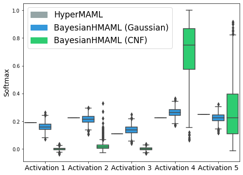
Figure 3: Predictions of HyperMAML, BayesianHMAML-G, and BayesianHMAML-CNF on out-of-distribution data. We trained the models on cross-domain data Omniglot$\rightarrow$EMNIST in a 5-shot setting, and then, for each of them, we sampled one thousand predictions. We show results on activations of 5 classes. Note, Bayesian models exhibit high uncertainty on out-of-distribution data. Furthermore, BayesianHMAML-CNF produces the most diverse predictions.

6 Conclusions

In this work, we introduced BayesianHMAML – a novel Bayesian Meta-Learning algorithm strongly motivated by MAML. In BayesianHMAML, we have universal weights trained in a point-wise manner, similar to MAML, and Bayesian updates modeled with hypernetworks. Such an approach allows for significantly larger updates in the adaptation phase and better uncertainty quantification. Our experiments show that BayesianHMAML outperforms all Bayesian and MAML-based methods in several standard Few-Shot learning benchmarks and in most cases, achieves results better or comparable to other state-of-the-art methods. Crucially, BayesianHMAML can be used to estimate the uncertainty of the predictions, enabling possible applications in critical areas of deep learning, such as medical diagnosis or autonomous driving.

7 Appendix: Training details

In this section, we present details of the training and architecture overview.

7.1 Architecture details

Encoder

For each experiment described in the main body of this work, we utilize a shallow convolutional encoder (feature extractor), commonly used in the literature (Finn et al., 2017; Chen et al., 2019; Patacchiola et al., 2020). This encoder consists of four convolutional layers, each consisting of a convolution, batch normalization, and ReLU nonlinearity. Each convolutional layer has an input and output size of 64, except for the first layer, where the input size equals the number of image channels. We also apply max-pooling between each convolution, decreasing the resolution of the processed feature maps by half. The output of the encoder is flattened to process it in the next layers.

In the case of the Omniglot and EMNIST images, such encoder compresses the images into 64-element embedding vectors, which serve as input to the Hypernetwork (with the above-described enhancements) and the classifier. However, in the case of substantially larger mini-ImageNet and CUB images, the backbone outputs a feature map of shape $[64\times 5\times 5]$, which would translate to $1600$-element embeddings and lead to an over parametrization of the Hypernetwork and classifier which processes them and increase the computational load. Therefore, we apply an average pooling operation to the obtained feature maps and ultimately also obtain embeddings of shape $64$. Thus, we can use significantly smaller Hypernetworks.

Hypernetwork

The Hypernetwork transforms the enhanced embeddings of the support examples of each class in a task into the updates for the portion of classifier weights predicting that class. It consists of three fully-connected layers with ReLU activation function between each consecutive pair of layers. In the hypernetwork, we use a hidden size of $256$ or $512$.

Classifier

The universal classifier is a single fully-connected layer with the input size equal to the encoder embedding size (in our case 64) and the output size equal to the number of classes. When using the strategy with embeddings enhancement, we freeze the classifier to get only the information about the behavior of the classifier. This means we do not calculate the gradient for the classifier in this step of the forward pass. Instead, gradient calculation for the classifier takes place during the classification of the query data.

7.2 Training details

In all of the experiments described in the main body of this work, we utilize the switch and the embedding enhancement mechanisms. We use the Adam optimizer and a multi-step learning rate schedule with the decay of $0.3$ and learning rate starting from $0.01$ or $0.001$. We train BayesianHMAML for 4000 epochs on all the data sets, save for the simpler Omniglot $\rightarrow$ EMNIST classification task, where we train for 2048 epochs instead.

7.3 Hyperparameters

Below, we outline the hyperparameters of architecture and training procedures used in each experiment.

hyperparameter	CUB	mini-ImageNet	mini-ImageNet $\rightarrow$ CUB	Omniglot $\rightarrow$ EMNIST
learning rate	$0.01$	$0.001$	$0.001$	$0.01$
Hyper Network depth	$3$	$3$	$3$	$3$
Hyper Network width	$512$	$256$	$256$	$512$
epochs no.	$4000$	$4000$	$4000$	$2048$
milestones	$51,550$	$101,1100$	$101,1100$	$51,550$
$\gamma$	$1e-4$	$1e-4$	$1e-5$	$0.001$
num. of samples (train)	$5$	$7$	$5$	$5$

Table 3: Hyperparameters for each of conducted 1-shot experiments. (G)

hyperparameter	CUB	mini-ImageNet	mini-ImageNet $\rightarrow$ CUB	Omniglot $\rightarrow$ EMNIST
learning rate	$0.001$	$0.001$	$0.001$	$0.01$
Hyper Network depth	$3$	$3$	$3$	$3$
Hyper Network width	$256$	$256$	$256$	$512$
epochs no.	$4000$	$4000$	$4000$	$2048$
milestones	$101,1100$	$101,1100$	$101,1100$	$51,550$
$\gamma$	$1e-5$	$1e-5$	$1e-4$	$0.001$
num. of samples (train)	$5$	$5$	$5$	$5$

Table 4: Hyperparameters for each of the conducted 5-shot experiments. (G)

hyperparameter	CUB	mini-ImageNet	mini-ImageNet $\rightarrow$ CUB	Omniglot $\rightarrow$ EMNIST
learning rate	$0.001$	$0.001$	$0.001$	$0.001$
Hyper Network depth	$3$	$3$	$3$	$3$
Hyper Network width	$512$	$256$	$256$	$512$
epochs no.	$4000$	$4000$	$4000$	$2048$
milestones	$51,550$	$101,1100$	$101,1100$	$51,550$
$\gamma$	$1e-6$	$1e-6$	$1e-6$	$1e-4$
num. of samples (train)	$5$	$5$	$5$	$5$

Table 5: Hyperparameters for each of conducted 1-shot experiments. (CNF)

hyperparameter	CUB	mini-ImageNet	mini-ImageNet $\rightarrow$ CUB	Omniglot $\rightarrow$ EMNIST
learning rate	$0.001$	$0.001$	$0.001$	$0.001$
Hyper Network depth	$3$	$3$	$3$	$3$
Hyper Network width	$256$	$256$	$256$	$512$
epochs no.	$4000$	$4000$	$4000$	$2048$
milestones	$101,1100$	$101,1100$	$101,1100$	$51,550$
$\gamma$	$1e-6$	$1e-6$	$1e-6$	$1e-6$
num. of samples (train)	$5$	$5$	$5$	$5$

Table 6: Hyperparameters for each of the conducted 5-shot experiments. (CNF)

8 Appendix: Extended results

We include an expanded version of Table 1 from the main manuscript in Table 7, comparing our approach to a larger number of meta-learning methods.

Table 7: Classification accuracy for inference on ${CUB}$ and ${mini-ImageNet}$ data sets in the $1$-shot and $5$-shot settings. The highest results are in bold and the second-highest in italic.

	CUB		mini-ImageNet
Method	1-shot	5-shot	1-shot	5-shot
ML-LSTM (Ravi and Larochelle, 2017)	–	–	$43.44\pm 0.77$	$60.60\pm 0.71$
SNAIL (Mishra et al., 2018)	–	–	$45.10$	$55.20$
Feature Transfer (Zhuang et al., 2020)	$46.19\pm 0.64$	$68.40\pm 0.79$	$39.51\pm 0.23$	$60.51\pm 0.55$
ProtoNet (Snell et al., 2017)	$52.52\pm 1.90$	$75.93\pm 0.46$	$44.19\pm 1.30$	$64.07\pm 0.65$
MAML (Finn et al., 2017)	$56.11\pm 0.69$	$74.84\pm 0.62$	$45.39\pm 0.49$	$61.58\pm 0.53$
MAML++ (Antoniou et al., 2018)	–	–	$52.15\pm 0.26$	${68.32\pm 0.44}$
FEAT (Ye et al., 2018)	$\mathbf{68.87\pm 0.22}$	$\mathbf{82.90\pm 0.15}$	$\mathbf{55.15\pm 0.20}$	$\mathbf{71.61\pm 0.16}$
LLAMA (Grant et al., 2018)	–	–	$49.40\pm 1.83$	–
VERSA (Gordon et al., 2018)	–	–	$48.53\pm 1.84$	$67.37\pm 0.86$
Amortized VI (Gordon et al., 2018)	–	–	$44.13\pm 1.78$	$55.68\pm 0.91$
Meta-Mixture (Jerfel et al., 2019)	–	–	$49.60\pm 1.50$	$64.60\pm 0.92$
Baseline++ (Chen et al., 2019)	$61.75\pm 0.95$	$78.51\pm 0.59$	$47.15\pm 0.49$	$66.18\pm 0.18$
MatchingNet (Vinyals et al., 2016)	$60.19\pm 1.02$	$75.11\pm 0.35$	$48.25\pm 0.65$	$62.71\pm 0.44$
RelationNet (Sung et al., 2018)	$62.52\pm 0.34$	$78.22\pm 0.07$	$48.76\pm 0.17$	$64.20\pm 0.28$
DKT + CosSim (Patacchiola et al., 2020)	$63.37\pm 0.19$	$77.73\pm 0.26$	$48.64\pm 0.45$	$62.85\pm 0.37$
DKT + BNCosSim (Patacchiola et al., 2020)	$62.96\pm 0.62$	$77.76\pm 0.62$	$49.73\pm 0.07$	$64.00\pm 0.09$
VAMPIRE (Nguyen et al., 2020)	–	–	$51.54\pm 0.74$	$64.31\pm 0.74$
PLATIPUS (Finn et al., 2018)	–	–	$50.13\pm 1.86$	–
ABML (Ravi and Beatson, 2018)	$49.57\pm 0.42$	$68.94\pm 0.16$	$45.00\pm 0.60$	–
OVE PG GP + Cosine (ML) (Snell and Zemel, 2020)	$63.98\pm 0.43$	$77.44\pm 0.18$	$50.02\pm 0.35$	$64.58\pm 0.31$
OVE PG GP + Cosine (PL) (Snell and Zemel, 2020)	$60.11\pm 0.26$	$79.07\pm 0.05$	$48.00\pm 0.24$	$67.14\pm 0.23$
FO-MAML (Nichol et al., 2018)	–	–	$48.70\pm 1.84$	$63.11\pm 0.92$
Reptile (Nichol et al., 2018)	–	–	$49.97\pm 0.32$	$65.99\pm 0.58$
VSM (Zhen et al., 2020)	–	–	$\mathit{54.73\pm 1.60}$	$68.01\pm 0.90$
PPA (Qiao et al., 2017)	–	–	$\mathit{54.53\pm 0.40}$	–
HyperShot (Sendera et al., 2022)	$65.27\pm 0.24$	$79.80\pm 0.16$	$52.42\pm 0.46$	$68.78\pm 0.29$
HyperShot+ adaptation (Sendera et al., 2022)	$66.13\pm 0.26$	$80.07\pm 0.22$	$53.18\pm 0.45$	$69.62\pm 0.2$
iMAML-HF (Rajeswaran et al., 2019)	–	–	$49.30\pm 1.88$	–
SignMAML (Fan et al., 2021)	–	–	$42.90\pm 1.50$	$60.70\pm 0.70$
Bayesian MAML (Yoon et al., 2018)	$55.93\pm 0.71$	–	${53.80\pm 1.46}$	$64.23\pm 0.69$
Unicorn-MAML (Ye and Chao, 2021)	–	–	$54.89$	–
Meta-SGD (Li et al., 2017)	–	–	$50.47\pm 1.87$	$64.03\pm 0.94$
MetaNet (Munkhdalai and Yu, 2017)	–	–	$49.21\pm 0.96$	–
PAMELA (Rajasegaran et al., 2020)	–	–	$53.50\pm 0.89$	$\mathit{70.51\pm 0.67}$
HyperMAML (Przewięźlikowski et al., 2022)	$66.11\pm 0.28$	$78.89\pm 0.19$	$51.84\pm 0.57$	$66.29\pm 0.43$
BayesianHMAML (G)	$66.57\pm 0.47$	$79.86\pm 0.31$	$52.54\pm 0.46$	$67.39\pm 0.35$
BayesianHMAML (G) + adaptation	$\mathit{66.92\pm 0.38}$	$\mathit{80.47\pm 0.38}$	$52.69\pm 0.38$	$68.24\pm 0.47$
BayesianHMAML (CNF)	$61.55\pm 0.69$	$75.41\pm 0.21$	$49.39\pm 0.33$	$64.77\pm 0.21$
BayesianHMAML (CNF) + adaptation	$62.15\pm 0.51$	$75.69\pm 0.32$	$49.61\pm 0.24$	$65.48\pm 0.43$

References

- Amit and Meir [2018] R. Amit and R. Meir. Meta-learning by adjusting priors based on extended pac-bayes theory. In International Conference on Machine Learning, pages 205–214. PMLR, 2018.
- Antoniou et al. [2018] A. Antoniou, H. Edwards, and A. Storkey. How to train your maml, 2018. URL https://arxiv.org/abs/1810.09502.
- Bauer et al. [2017] M. Bauer, M. Rojas-Carulla, J. B. Światkowski, B. Schölkopf, and R. E. Turner. Discriminative k-shot learning using probabilistic models, 2017.
- Bengio et al. [1992] S. Bengio, Y. Bengio, J. Cloutier, and J. Gecsei. On the optimization of a synaptic learning rule. 1992.
- Blundell et al. [2015] C. Blundell, J. Cornebise, K. Kavukcuoglu, and D. Wierstra. Weight uncertainty in neural network. In International conference on machine learning, pages 1613–1622. PMLR, 2015.
- Bowman et al. [2016] S. R. Bowman, L. Vilnis, O. Vinyals, A. M. Dai, R. Jozefowicz, and S. Bengio. Generating sentences from a continuous space. In 20th SIGNLL Conference on Computational Natural Language Learning, CoNLL 2016, pages 10–21. Association for Computational Linguistics (ACL), 2016.
- Chen and Chen [2022] L. Chen and T. Chen. Is bayesian model-agnostic meta learning better than model-agnostic meta learning, provably? In International Conference on Artificial Intelligence and Statistics, pages 1733–1774. PMLR, 2022.
- Chen et al. [2018] T. Q. Chen, Y. Rubanova, J. Bettencourt, and D. K. Duvenaud. Neural ordinary differential equations. In NeurIPS, pages 6571–6583, 2018.
- Chen et al. [2019] W.-Y. Chen, Y.-C. Liu, Z. Kira, Y.-C. F. Wang, and J.-B. Huang. A closer look at few-shot classification. arXiv preprint arXiv:1904.04232, 2019.
- Ding et al. [2021] N. Ding, X. Chen, T. Levinboim, S. Goodman, and R. Soricut. Bridging the gap between practice and pac-bayes theory in few-shot meta-learning. Advances in Neural Information Processing Systems, 34:29506–29516, 2021.
- Dinh et al. [2014] L. Dinh, D. Krueger, and Y. Bengio. Nice: Non-linear independent components estimation. arXiv preprint arXiv:1410.8516, 2014.
- Fan et al. [2021] C. Fan, P. Ram, and S. Liu. Sign-maml: Efficient model-agnostic meta-learning by signsgd. CoRR, abs/2109.07497, 2021.
- Farid and Majumdar [2021] A. Farid and A. Majumdar. Generalization bounds for meta-learning via pac-bayes and uniform stability. Advances in Neural Information Processing Systems, 34:2173–2186, 2021.
- Finn et al. [2017] C. Finn, P. Abbeel, and S. Levine. Model-agnostic meta-learning for fast adaptation of deep networks. In International Conference on Machine Learning, pages 1126–1135. PMLR, 2017.
- Finn et al. [2018] C. Finn, K. Xu, and S. Levine. Probabilistic model-agnostic meta-learning. Advances in neural information processing systems, 31, 2018.
- Gordon et al. [2018] J. Gordon, J. Bronskill, M. Bauer, S. Nowozin, and R. Turner. Meta-learning probabilistic inference for prediction. In International Conference on Learning Representations, 2018.
- Gordon et al. [2019] J. Gordon, J. Bronskill, M. Bauer, S. Nowozin, and R. Turner. Meta-learning probabilistic inference for prediction. In International Conference on Learning Representations (ICLR 2019). OpenReview. net, 2019.
- Grant et al. [2018] E. Grant, C. Finn, S. Levine, T. Darrell, and T. Griffiths. Recasting gradient-based meta-learning as hierarchical bayes. In International Conference on Learning Representations, 2018.
- Grathwohl et al. [2018] W. Grathwohl, R. T. Chen, J. Bettencourt, I. Sutskever, and D. Duvenaud. Ffjord: Free-form continuous dynamics for scalable reversible generative models. In International Conference on Learning Representations, 2018.
- Ha et al. [2016] D. Ha, A. Dai, and Q. V. Le. Hypernetworks. arXiv preprint arXiv:1609.09106, 2016.
- Hospedales et al. [2020] T. Hospedales, A. Antoniou, P. Micaelli, and A. Storkey. Meta-learning in neural networks: A survey. 2020.
- Jerfel et al. [2019] G. Jerfel, E. Grant, T. L. Griffiths, and K. Heller. Reconciling meta-learning and continual learning with online mixtures of tasks. In Proceedings of the 33rd International Conference on Neural Information Processing Systems, pages 9122–9133, 2019.
- Kingma and Dhariwal [2018] D. P. Kingma and P. Dhariwal. Glow: Generative flow with invertible 1x1 convolutions. In NeurIPS, pages 10215–10224, 2018.
- Lee et al. [2019] K. Lee, S. Maji, A. Ravichandran, and S. Soatto. Meta-learning with differentiable convex optimization. In Proceedings of the IEEE/CVF Conference on Computer Vision and Pattern Recognition, pages 10657–10665, 2019.
- Li et al. [2017] Z. Li, F. Zhou, F. Chen, and H. Li. Meta-sgd: Learning to learn quickly for few-shot learning, 2017.
- MacKay [1992] D. J. MacKay. A practical bayesian framework for backpropagation networks. Neural computation, 4(3):448–472, 1992.
- Mishra et al. [2018] N. Mishra, M. Rohaninejad, X. Chen, and P. Abbeel. A simple neural attentive meta-learner. In International Conference on Learning Representations, 2018.
- Munkhdalai and Yu [2017] T. Munkhdalai and H. Yu. Meta networks. In International Conference on Machine Learning, pages 2554–2563. PMLR, 2017.
- Nguyen et al. [2020] C. Nguyen, T.-T. Do, and G. Carneiro. Uncertainty in model-agnostic meta-learning using variational inference. In Proceedings of the IEEE/CVF Winter Conference on Applications of Computer Vision, pages 3090–3100, 2020.
- Nichol et al. [2018] A. Nichol, J. Achiam, and J. Schulman. On first-order meta-learning algorithms. arXiv preprint arXiv:1803.02999, 2018.
- Oreshkin et al. [2018] B. N. Oreshkin, P. Rodriguez, and A. Lacoste. Tadam: Task dependent adaptive metric for improved few-shot learning. arXiv preprint arXiv:1805.10123, 2018.
- Patacchiola et al. [2020] M. Patacchiola, J. Turner, E. J. Crowley, M. O’Boyle, and A. J. Storkey. Bayesian meta-learning for the few-shot setting via deep kernels. Advances in Neural Information Processing Systems, 33, 2020.
- Przewięźlikowski et al. [2022] M. Przewięźlikowski, P. Przybysz, J. Tabor, M. Zięba, and P. Spurek. Hypermaml: Few-shot adaptation of deep models with hypernetworks. arXiv preprint arXiv:2205.15745, 2022.
- Qiao et al. [2017] S. Qiao, C. Liu, W. Shen, and A. Yuille. Few-shot image recognition by predicting parameters from activations, 2017.
- Rajasegaran et al. [2020] J. Rajasegaran, S. H. Khan, M. Hayat, F. S. Khan, and M. Shah. Meta-learning the learning trends shared across tasks. CoRR, abs/2010.09291, 2020. URL https://arxiv.org/abs/2010.09291.
- Rajeswaran et al. [2019] A. Rajeswaran, C. Finn, S. M. Kakade, and S. Levine. Meta-learning with implicit gradients. Advances in Neural Information Processing Systems, 32:113–124, 2019.
- Rasmussen [2003] C. E. Rasmussen. Gaussian processes in machine learning. In Summer school on machine learning, pages 63–71. Springer, 2003.
- Ravi and Beatson [2018] S. Ravi and A. Beatson. Amortized bayesian meta-learning. In International Conference on Learning Representations, 2018.
- Ravi and Larochelle [2017] S. Ravi and H. Larochelle. Optimization as a model for few-shot learning. In ICLR, 2017.
- Rothfuss et al. [2020] J. Rothfuss, M. Josifoski, and A. Krause. Meta-learning bayesian neural network priors based on pac-bayesian theory. 2020.
- Rothfuss et al. [2021] J. Rothfuss, V. Fortuin, M. Josifoski, and A. Krause. Pacoh: Bayes-optimal meta-learning with pac-guarantees. In International Conference on Machine Learning, pages 9116–9126, 2021.
- Rusu et al. [2018] A. A. Rusu, D. Rao, J. Sygnowski, O. Vinyals, R. Pascanu, S. Osindero, and R. Hadsell. Meta-learning with latent embedding optimization. In International Conference on Learning Representations, 2018.
- Schmidhuber [1992] J. Schmidhuber. Learning to Control Fast-Weight Memories: An Alternative to Dynamic Recurrent Networks. Neural Computation, 4(1):131–139, 01 1992. ISSN 0899-7667.
- Sendera et al. [2021] M. Sendera, J. Tabor, A. Nowak, A. Bedychaj, M. Patacchiola, T. Trzcinski, P. Spurek, and M. Zieba. Non-gaussian gaussian processes for few-shot regression. Advances in Neural Information Processing Systems, 34:10285–10298, 2021.
- Sendera et al. [2022] M. Sendera, M. Przewięźlikowski, K. Karanowski, M. Zięba, J. Tabor, and P. Spurek. Hypershot: Few-shot learning by kernel hypernetworks. arXiv preprint arXiv:2203.11378, 2022.
- Snell and Zemel [2020] J. Snell and R. Zemel. Bayesian few-shot classification with one-vs-each pólya-gamma augmented gaussian processes. In International Conference on Learning Representations, 2020.
- Snell et al. [2017] J. Snell, K. Swersky, and R. S. Zemel. Prototypical networks for few-shot learning. arXiv preprint arXiv:1703.05175, 2017.
- Sung et al. [2018] F. Sung, Y. Yang, L. Zhang, T. Xiang, P. H. Torr, and T. M. Hospedales. Learning to compare: Relation network for few-shot learning. In Proceedings of the IEEE conference on computer vision and pattern recognition, pages 1199–1208, 2018.
- Vinyals et al. [2016] O. Vinyals, C. Blundell, T. Lillicrap, D. Wierstra, et al. Matching networks for one shot learning. Advances in neural information processing systems, 29:3630–3638, 2016.
- Wang et al. [2020] Y. Wang, Q. Yao, J. Kwok, and L. M. Ni. Generalizing from a few examples: A survey on few-shot learning, 2020.
- Wang et al. [2021] Z. Wang, Z. Miao, X. Zhen, and Q. Qiu. Learning to learn dense gaussian processes for few-shot learning. Advances in Neural Information Processing Systems, 34, 2021.
- Ye et al. [2018] H. Ye, H. Hu, D. Zhan, and F. Sha. Learning embedding adaptation for few-shot learning. CoRR, abs/1812.03664, 2018.
- Ye and Chao [2021] H.-J. Ye and W.-L. Chao. How to train your maml to excel in few-shot classification, 2021.
- Yoon et al. [2018] J. Yoon, T. Kim, O. Dia, S. Kim, Y. Bengio, and S. Ahn. Bayesian model-agnostic meta-learning. In Proceedings of the 32nd International Conference on Neural Information Processing Systems, pages 7343–7353, 2018.
- Zhao et al. [2020] D. Zhao, J. von Oswald, S. Kobayashi, J. Sacramento, and B. F. Grewe. Meta-learning via hypernetworks. 2020.
- Zhen et al. [2020] X. Zhen, Y.-J. Du, H. Xiong, Q. Qiu, C. Snoek, and L. Shao. Learning to learn variational semantic memory. In NeurIPS, 2020.
- Zhmoginov et al. [2022] A. Zhmoginov, M. Sandler, and M. Vladymyrov. Hypertransformer: Model generation for supervised and semi-supervised few-shot learning. In International Conference on Machine Learning, pages 27075–27098. PMLR, 2022.
- Zhuang et al. [2020] F. Zhuang, Z. Qi, K. Duan, D. Xi, Y. Zhu, H. Zhu, H. Xiong, and Q. He. A comprehensive survey on transfer learning, 2020.