Learning Consistency-Aware Unsigned Distance Functions Progressively from Raw Point Clouds

Abstract

Surface reconstruction for point clouds is an important task in 3D computer vision. Most of the latest methods resolve this problem by learning signed distance functions (SDF) from point clouds, which are limited to reconstructing shapes or scenes with closed surfaces. Some other methods tried to represent shapes or scenes with open surfaces using unsigned distance functions (UDF) which are learned from large scale ground truth unsigned distances. However, the learned UDF is hard to provide smooth distance fields near the surface due to the noncontinuous character of point clouds. In this paper, we propose a novel method to learn consistency-aware unsigned distance functions directly from raw point clouds. We achieve this by learning to move 3D queries to reach the surface with a field consistency constraint, where we also enable to progressively estimate a more accurate surface. Specifically, we train a neural network to gradually infer the relationship between 3D queries and the approximated surface by searching for the moving target of queries in a dynamic way, which results in a consistent field around the surface. Meanwhile, we introduce a polygonization algorithm to extract surfaces directly from the gradient field of the learned UDF. The experimental results in surface reconstruction for synthetic and real scan data show significant improvements over the state-of-the-art under the widely used benchmarks. Project page: https://junshengzhou.github.io/CAP-UDF.

1 Introduction

Reconstructing surfaces from 3D point clouds is vital in 3D vision, robotics and graphics. It bridges the gap between raw point clouds that can be captured by 3D sensors and the editable surfaces for various downstream applications. Recently, Neural Implicit Functions (NIFs) have achieved promising results by training deep networks to learn Signed Distance Functions (SDFs) [44, 26, 42, 14] or occupancies [40, 46, 41, 10], and then extract a polygon mesh of a continuous iso-surface from a discrete scalar field using the marching cubes algorithm [35]. However, the NIFs approaches based on learning internal and external relations can only reconstruct closed surfaces. The limitation prevents NIFs from representing most real-world objects such as cars with inner structures, clothes with unsealed ends or 3D scenes with open walls and holes.

As a remedy, state-of-the-art methods [12, 62, 49] learn Unsigned Distance Functions (UDFs) as a more general representation to reconstruct surfaces from point clouds. However, these methods can not learn UDFs with smooth distance fields near surfaces, due to the noncontinuous character of point clouds, even using ground truth distance values or large scale meshes during training. Moreover, most UDF approaches failed to extract surfaces directly from unsigned distance fields. Particularly, they rely on post-processing such as Ball-Pivoting-Algorithm (BPA) [3] to extract surfaces based on the dense point clouds generated from the learned UDF, which is very time-consuming and also leads to surfaces with discontinuity and poor quality.

To solve these issues, we propose a novel method to learn consistency-aware UDFs directly from raw point clouds. We learn to move 3D queries to reach the approximated surface aggressively with a field consistency constraint, and introduce a polygonization algorithm to extract surfaces from the learned unsigned distance functions in a new perspective. Our method can learn UDFs from a single point cloud without requiring ground truth distances, point normals, or a large scale training set. Specifically, given query locations sampled in 3D space as input, We learn to move them to the approximated surface according to the predicted unsigned distances and the gradient at the query locations. More appealing solutions [1, 2, 20, 36] have been proposed to learn SDFs from raw point clouds by optimizing the relationship between the query point and its closest point in raw data as a surface prior. However, since the raw point cloud is a highly discrete approximation of the surface, the closest point to the query location is always inaccurate and ambiguous, which makes the network difficult to converge to an accurate UDF due to the inconsistent or even conflicting optimization directions in the distance field.

Therefore, in order to encourage the network to learn a consistency-aware and accurate unsigned distance field, we propose to dynamically search the optimization target with a specially designed loss function containing field consistency to mimic the conflict optimizations. We also progressively infer the mapping between 3D queries and the approximated zero iso-surface by using well-moved queries as additional priors for promoting further convergence. To extract a surface in a direct way, we propose to use the gradient field of the learned UDFs to determine whether two queries are on the same side of the approximated surface or not. In contrast to NDF [12] which also learns UDFs but takes dense point clouds as output and depends on BPA [3] to generate meshes, our method shows great advantages in efficiency and accuracy due to the straightforward surface extraction.

Our main contributions can be summarized as:

• We propose a novel neural network that learns consistent-aware UDFs directly from raw point clouds. Our method gradually infers the relationship between 3D query locations and the approximated surface with a field consistent loss.

• We introduce an algorithm for directly extracting high-fidelity iso-surfaces with arbitrary topology from the gradient field of the learned unsigned distance functions.

• We obtain state-of-the-art results in surface reconstruction from synthetic and real scan point clouds under the widely used benchmarks.

2 Related Works

Surface reconstruction from 3D point clouds has been studied for decades. Classic optimization-based methods [15, 3, 28, 29] tried to resolve this problem by inferring continuous surfaces from the geometry of point clouds. With the rapid development of deep learning [63, 33, 56, 61, 27, 24, 54, 55, 58, 53], the neural networks have shown great potential in reconstructing 3D surfaces [30, 9, 8, 22, 13, 17, 51, 43, 31, 52]. In the following, we will briefly review the studies of deep learning based methods.

2.1 Neural Implicit Surface Reconstruction

In the past few years, a lot of advances have been made in 3D surface reconstruction with Neural Implicit Functions (NIFs). The NIFs approaches [7, 25, 46, 40, 16, 26, 32, 41, 34, 44, 39] use either binary occupancies [40, 46, 41, 10] or signed distance functions (SDFs) [44, 26, 42, 14] to represent 3D shapes or scenes, and then use marching cubes [35] algorithm to reconstruct the learned implicit functions into surfaces. Earlier works [40, 44, 25, 10] use an encoder [40, 10] or an optimization based method [44] to embed the shape into a global latent code, and then use a decoder to reconstruct the shape. To obtain more detailed geometry, some methods [18, 19, 48, 7, 11, 26, 41, 38, 37] proposed to leverage more latent codes to capture local shape priors. To achieve this, the point cloud is first split into different uniform grids [7, 11, 26] or local patches [18, 19, 48], and a neural network is then used to extract a latent code for each grid/patch. Some recent works propose to learn NIFs from a new perspective, such as implicit moving least-squares surfaces [32], differentiable poisson solver [45], iso-points [60] , point convolution [6] or predictive context learning [38]. However, the NIFs approaches can only represent closed shapes due to the characters of occupancies and SDFs.

2.2 Learning Unsigned Distance Functions

To model general shapes with open and multi-layer surfaces, NDF [12] learns unsigned distance functions to represent shapes by predicting the unsigned distance from a query location to the continuous surface. However, NDF merely predicts dense point clouds as the output, which requires time-consuming post-processing for mesh generation and also struggles to retain high-quality details of shapes. In contrast, our method is able to extract surfaces directly from the gradient field of the learned UDFs. Following works use image features [62] or query side relations [59] as additional constraints to improve reconstruction accuracy, some other works advance UDFs for normal estimation [49] or semantic segmentation [50]. However, these methods require ground truth distance values or even a large scale meshes during training and are hard to provide smooth distance fields near the surface due to the noncontinuous character of point clouds. While our method does not require any additional supervision but raw point clouds during training, which allows us to reconstruct surfaces for real point cloud scans. In a differential manner, a concurrent work named MeshUDF [21] meshes UDFs from the dynamic gradients during training with a voting schema. On the contrary, we learn a consistancy-aware UDF first and extract the surface from stable gradients during testing. Moreover, our surface extraction algorithm is simpler to use, which is implemented in the marching cube algorithm.

2.3 Surface Reconstruction from Raw Point Clouds

Learning implicit functions directly from raw point clouds without ground truth signed/unsigned distance values or occupancy values is more challenge. Current works introduce sign agnostic learning with a specially designed network initialization [1], constraints on gradients [2] or geometric regularization [20] for learning SDFs from raw data. Neural-Pull [36] uses a new way of learning SDFs by pulling nearby space onto the surface. However, they aim to learn signed distances and hence can not reconstruct complex shapes with open or multi-layer surfaces. In contrast, our method is able to learn a continuous unsigned distance function from point clouds, which allows us to reconstruct surfaces for shapes and scenes with arbitrary typology.

3 Method

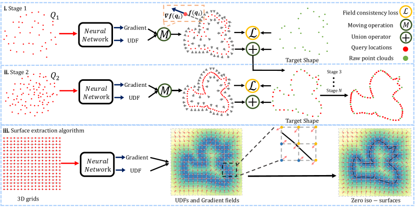
Figure 1: Overview of our method. Given a 3D query $q_{i}\in{Q_{1}}$ as input, the neural network predicts the unsigned distance $f(q_{i})$ of $q_{i}$ and moves $q_{i}$ against the direction of gradient at $q_{i}$ with a stride of $f(q_{i})$. The field consistency loss is then computed between the moved queries $q^{\prime}_{i}$ and the target point cloud $P$ as the optimization target. After the network converges in the current stage, we update $P$ with a subset of $q^{\prime}_{i}$ as additional priors to learn more local details in the next stage. Finally, we use the gradient field of the learned UDFs to model the relationship between different 3D grids and extract iso-surfaces directly.

Problem statement. We design a neural network to learn UDFs that represents 3D shapes. Given a 3D query location $q=[x,y,z]$, a learned UDF $f$ predicts the unsigned distance value $s=f(q)\in\mathbb{R}$. Current methods depend on ground truth distance values generated from continuous surfaces and employ a neural network to learn $f$ as a regression problem. Different from these methods, we aim to learn $f$ directly from a raw point cloud $P=\{p_{i},i\in[1,N]\}$. Furthermore, these methods require post-processing [12] or additional supervision [59] to generate meshes. On the contrary, we introduce an algorithm to extract surfaces directly from $f$ using the gradient field $\nabla f$. The overview of our method is shown in Fig. 1.

3.1 Learn UDFs from Raw Point Clouds

We introduce a novel neural network to learn a continuous UDF $f$ from a raw point cloud. We demonstrate our idea using a 2D point cloud $S$ in Fig. 1(a), where $S$ indicates some discrete points of a continuous surface. Specifically, given a set of query locations $Q=\{q_{i},i\in[1,M]\}$ which is randomly sampled around $S$, the network moves $q_{i}$ against the direction of the gradient $g_{i}$ at $q_{i}$ with a stride of predicted unsigned distance value $f(q_{i})$. The gradient $g_{i}$ is a vector that presents the partial derivative of $f$ at $q_{i}=[x_{i},y_{i},z_{i}]$, which can be formulated as $g_{i}=\nabla f(q_{i})=[{\partial f}/{\partial x},{\partial f}/{\partial y},{\partial f}/{\partial z}]$. The direction of $g_{i}$ indicates the orientation of where the unsigned distance increases the fastest in 3D space, which points the direction away from the surface, therefore moving $q_{i}$ against the direction of $g_{i}$ will find a path to reach the surface of $S$. The moving operation can be formulated as:

$$z_{i}=q_{i}-f(q_{i})\times\nabla f(q_{i})/||\nabla f(q_{i})||_{2},$$ (1)

where $z_{i}$ is the location of the moved query $q_{i}$, and $\nabla f(q_{i})/||\nabla f(q_{i})||_{2}$ is the normalized gradient $g_{i}$, which indicates the direction of $g_{i}$. The moving operation is differentiable in both the unsigned distance value and the gradient, which allows us to optimize them simultaneously during training.

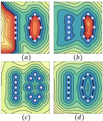
Figure 2: The level-sets show the distance fields learned by (a) Neural-Pull, (b) SAL, (c) NDF, (d) Ours. The color of blue and red represent positive or negative distance. The darker the color, the closer it is to the approximated surface.

The four examples in Fig. 2 show the distance fields learned by Neural-Pull [36], SAL [1], NDF [12] and our method for a sparse 2D point cloud $P$ which only contains 13 points. One main branch to learn signed or unsigned distance functions for point clouds is to directly minimize the mean squared error between the predicted distance value $f(q_{i})$ and the euclidean distance between $q_{i}$ and its nearest neighbour in $P$, as proposed in NDF and SAL. However, as shown in Fig. 2(c), NDF leads to an extremely discrete distance field. To learn a continuous distance field, NDF introduces ground truth distance values extracted from the continuous surface as extra supervision, which prevents it from learning directly from raw point clouds. SAL shows a great capacity in learning SDFs for watertight shapes using a carefully designed initialization. However, as shown in Fig. 2(b), SAL fails to converge to a multi-structure shape since the network is initialized as a single layer shape prior. Neural-Pull uses a similar way as ours to pull queries onto the surface, thus also learns a continuous signed distance field as shown in Fig. 2(a). However, the nature of SDF prevents Neural-Pull from reconstructing open surfaces like the $``1"$ on the left of Fig. 2(a). As shown in Fig. 2(d), our method can learn a continuous level set of distance field and can also represent open surfaces.

One way to extend Neural-Pull directly to learn UDFs is to predict a positive distance value for each query and pull it to the nearest neighbour in $P$. However, for shapes with complex topology, this optimization is often ambiguous due to the noncontinuous character of raw point clouds. We solve this problem by introducing consistency-aware field learning.

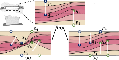
Figure 3: Demonstration case of different losses.

3.2 Consistency-Aware Field Learning

Neural-Pull leverages a mean squared error to minimize the distance between the moved query $z_{i}$ and the nearest neighbour $n_{i}$ of $q_{i}$ in $P$:

$$\mathcal{L}=\frac{1}{M}\sum_{i\in[1,M]}{||z_{i}-n_{i}||_{2}^{2}}.$$ (2)

However, the direct optimization of the loss in Eq. (2) will form a distorted field and lead some queries to get stuck due to the conflict optimization which makes the network difficult to converge. We show a 2D case of learning UDFs for a double-deck wall using the loss Eq. (2) as in Fig. 3(b) and using our loss as in Fig. 3(c). Assume $p_{1}$ and $p_{2}$ as two discrete points in two different decks of the wall, $q_{1}$ and $q_{2}$ are two queries whose closest neighbours are $p_{1}$ and $p_{2}$, respectively. Optimizing the network using $q_{1}$ and $q_{2}$ by minimizing Eq. (2) or our proposed loss in Eq. (3) will lead to an unsigned distance field as in Fig. 3(a). Assuming in the next training batch, $q_{3}$ and $q_{4}$ are two queries whose closest neighbours are $p_{3}$ and $p_{4}$. If we use the loss in Eq. (2), the optimization target of $q_{3}$ is to minimize $\mathcal{L}={||z_{3}-p_{3}||_{2}^{2}}$. Notice that the target point $p_{3}$ is located on the lower surface, however the opposite direction of gradient around $q_{3}$ is upward at this moment. Therefore, the partial derivative $\frac{\partial\mathcal{L}}{\partial z_{3}}$ leads to a decrease in the unsigned distance value $f(q_{3})$ predicted by the network. The case of $q_{4}$ is optimized similarly. An immediate consequence is that the inconsistent optimization directions will form a distorted fields that has local minima of unsigned distance values at $q_{3}$ and $q_{4}$ as in Fig. 3(b). However, this situation causes other query points around point $q_{3}$ or $q_{4}$ to get stuck in the distorted fields and unable to move to the correct location, thus making the network hard to converge.

To address this issue, we propose a loss function which can keep the consistency of unsigned distance fields to avoid the conflicting optimization directions. Specifically, instead of strictly constraining the convergence target before forward propagation as Eq. (2), we first predict the moving path of a query location $q_{i}$ and move it using Eq. (1) to $z_{i}$, then look for the surface point $p_{i}$ in $P$ which is the closest to $z_{i}$ and minimize the distance between $z_{i}$ and $p_{i}$. As shown in Fig. 3(c), after moving $q_{3}$ against the gradient direction with a stride of $f(q_{3})$ to $z_{3}$, the closest surface point of $z_{3}$ lies on the upper deck, so the distance fields remain continuous and are optimized correctly. In practical, we use chamfer distance as a suitable loss implementation, formulated as:

$$\mathcal{L}_{\rm CD}=\frac{1}{M}\sum_{i\in[1,M]}\mathop{min}\limits_{j\in[1,N]}{||z_{i}-p_{j}||_{2}}+\frac{1}{N}\sum_{j\in[1,N]}\mathop{min}\limits_{i\in[1,M]}{||p_{j}-z_{i}||_{2}}.$$ (3)

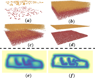
Figure 4: Advantages of our loss.

We also use toy examples as shown in Fig. 4 to show the advantage of our proposed field consistency loss. We learn UDFs for a raw point cloud of a double-deck wall as shown in Fig. 4(a). Fig. 4(b) denotes the randomly sampled query locations between two decks of the wall where the different colors mean the queries are closer to the upper or lower deck of the wall. Fig. 4(c) and Fig. 4(d) indicate the moved queries by loss in Eq. (2) and Eq. (3). It can be seen that our proposed loss can move most of the queries to the correct surface position, and Neural-Pull loss stops moving in many places or moves queries to the wrong places due to the field inconsistency in optimization. Fig. 4(e) and Fig. 4(f) show the learned distance field of a car with inner structure by the loss in Eq. (2) and our loss.

3.3 Progressive Surface Approximation

Moreover, in order to predict unsigned distance values more accurately and learn more local details, we propose a progressive learning strategy by taking the intermediate results of moved queries as additional priors. Given a raw point cloud which is a discrete representation of the surface, we have made a reasonable assumption: the closer the query location is to the given point cloud, the smaller the error of searching the target point on the given point cloud. We provide the Proof of this assumption in the appendix. Based on this assumption, we set up two regions: the high confidence region with small error and the low confidence region with large error. We sample query points in the high confidence region to help train the network and sample auxiliary points in the low confidence region to move to the estimated surface position by network gradient after network convergence at current stage, where the moved auxiliary points are regarded as the surface prior for the next stage. Notably, the auxiliary points do not participate in network training since these points with low confidence will lead to a large error and affect network training. Since the low confidence regions which are not optimized explicitly during training are distributed interspersed between the high confidence regions, according to the integral Monotone Convergence Theorem [5], the UDFs and gradient predicted by the low confidence region are a smooth expression of the trained high confidence region. We save the moved queries and auxiliary points and use them to update $S$. According to the updated point cloud, we re-divide the regions with high confidence and low confidence and re-sample the query points and auxiliary points for the next stage.

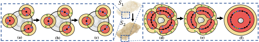
Figure 5: Illustration of progressively approximating the surface.

We demonstrate our idea using a 2D case in Fig. 5.(a). We divided the regions with high confidence (red region) and low confidence (yellow region) based on the given raw point cloud $S_{1}$ (black dots) and then sample query points $Q_{1}=\{q_{i},i\in[1,M]\}$ (blue dots) and auxiliary points(green dots) $A_{1}=\{a_{i},i\in[1,M]\}$. (b) We train the network to learn UDFs by moving the query locations $Q_{1}$ using Eq. (1), and optimize the network by minimizing Eq. (3). (c) After network convergence at current stage, we move query points $Q$ and auxiliary points $A$ to the estimated surface position by the gradient of network, $S_{1}^{{}^{\prime}}=p-f(p)\times\nabla f(p)/||\nabla f(p)||_{2},p\subset Q_{1}\cup A_{1}$. (d) We save the moved points $S_{1}^{{}^{\prime}}$ and use them to update $S$, $S_{2}=S_{1}\cup S_{1}^{{}^{\prime}}$. According to the updated point cloud $S_{2}$, we re-divided the regions with high confidence and low confidence and re-sampled the query points $Q_{2}$ and auxiliary points $A_{2}$. (e) We continue to train the network by moving query points $Q_{2}$ to the updated $S_{2}$, and then update $S$ by combining the moved $Q_{2}$ and $A_{2}$ with $S_{2}$. (f) Because of the more continuous surface prior information, the network will learn more accurately and learn more local details of the UDFs.

3.4 Surface Extraction Algorithm

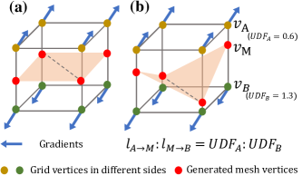
Figure 6: Surface extraction algorithm.

Unlike SDFs, UDFs fail to extract surfaces by marching cubes since UDFs cannot perform inside/outside tests on 3D grids. To address this issue, we propose to use the gradient field $\nabla f$ to determine whether two 3D grid locations are on the same side or the opposite side of the surface approximated by the point clouds $P$. We make an assumption that on a micro-scale of the surface, the space can always be divided into two sides, where the 3D query locations of different sides denoted as $Q_{in}=\{{q_{in}}^{i},i\in[1,L]\}$ and $Q_{out}=\{{q_{out}}^{i},i\in[1,I]\}$. For two queries ${q_{in}}^{i}$ and ${q_{out}}^{j}$ in different sides of the surface, the included angle between the directions of the gradients $\nabla f({q_{in}}^{i})$ and $\nabla f({q_{out}}^{j})$ are always more than 90 degrees, which can be formulated as $\nabla f({q_{in}}^{i})\cdot\nabla f({q_{out}}^{j})<0$. On the contrary, for two queries ${q_{in}}^{i}$ and ${q_{in}}^{j}$ in the same side, the formula $\nabla f({q_{in}}^{i})\cdot\nabla f({q_{in}}^{j})>0$ holds true. So, we can classify whether two points are in the same or the opposite side using dot product of gradients, $cls(q_{i},q_{j})=\nabla f(q_{i})\cdot\nabla f(q_{j})$. Based on that, we divide the space into 3D grids (e.g. $256^{3}$), and perform gradient discrimination on the 8 vertices $v_{i}$ in each cell grid according to the gradient field $\nabla f$ using $cls(q_{i},q_{j})$. As shown in Fig. 6(a), the gradient field separates the vertices into two sets, where we can further adapt marching cubes algorithm [35] to create triangles for the grid using the lookup table. The complete surface is generated by grouping triangles of each grid together. To accelerate the surface extraction process and avoid extracting unexpected triangles in the multi-layers structures, we set a threshold $\theta$ to stop surface extraction on grids where $f(g_{i})>\theta,i\in[0,7]$.

Mesh refinement. The initial surface extracted by marching cubes is only a discrete approximation of the zero iso-surface. To achieve a more detailed mesh, we propose to refine it using the UDF values. As shown in Fig. 6(b), given the predicted UDF values $UDF_{A}$ and $UDF_{B}$ of grid vertex $v_{A}$ and $v_{b}$, the mesh vertex $v_{M}$ can be moved to a finer position where $l_{A\rightarrow M}:l_{M\rightarrow B}=UDF_{A}:UDF_{B}$.

4 Experiments

We evaluate our method on the task of surface reconstruction from raw point clouds. We first demonstrate the ability of our method to reconstruct general shapes with open and multi-layer surfaces in Sec.4.1. Next, we apply our method to reconstruct surfaces for real scanned raw data including 3D objects in Sec.4.2 and complex scenes in Sec.4.3. Ablation studies are shown in Sec.4.4.

Implementation details. To learn UDFs for raw point clouds $P$, we adopt a neural network similar to OccNet [40] to predict the unsigned distance given 3D queries as input. Our network contains 8 layers of MLP where each layer has 256 nodes. Similar to Neural-Pull and SAL, given the single point cloud $P$ as input, we do not leverage any condition and overfit the network to approximate the surface of $P$ by minimizing the loss of Eq. (3). Therefore, we do not need to train our network on large scale training dataset in contrast to previous methods [12, 59, 26]. In addition, we use the same strategy as Neural-Pull to sample 60 queries around each point $p_{i}$ on $P$ as training data. A Gaussian function $\mathcal{N}(\mu,\sigma^{2})$ is adopt to calculate the sampling probability where $\mu=p_{i}$ and $\sigma$ is the distance between $p_{i}$ and its 50-th nearest points on $P$. For sampling auxiliary points in the low confidence region, the standard deviation is set to $1.1\sigma$. And we train our network for two stages in practice.

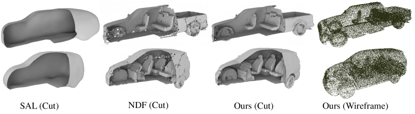
Figure 7: Visual comparisons of surface reconstruction on ShapeNet cars.

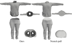
Figure 8: Visual comparisons on MGD dataset.

	Chamfer-L2		F-Score
Method	Mean	Median	$F1^{0.005}$	$F1^{0.01}$
Input	0.363	0.355	48.50	88.34
Watertight GT	2.628	2.293	68.82	81.60
GT	0.076	0.074	95.70	99.99
NDFBPA [12]	0.202	0.193	77.40	97.97
NDFgradRA	0.160	0.152	82.87	99.35
NDFPC	0.126	0.120	88.09	99.54
GIFS [59]	0.128	0.123	88.05	99.31
OursBPA	0.141	0.138	84.84	99.33
OursgradRA	0.119	0.114	88.55	99.82
OursPC	0.110	0.106	90.06	99.87

Table 1: Comparison on ShapeNet cars.

4.1 Surface Reconstruction for Synthetic Shapes

Dataset and metrics. For the experiments on synthetic shapes, we follow NDF [12] to choose the “Car" category of the ShapeNet dataset which contains the greatest amount of multi-layer shapes and non-closed shapes. And 10k points is sampled from the surface of each shape as the input. Besides, we employ the MGD dataset [4] to show the advantage of our method in open surfaces. To measure the reconstruction quality, we follow GIFS [59] to sample 100k points from the reconstructed surfaces and adopt the Chamfer distance ($\times 10^{4}$), Normal Consistency (NC) [40] and F-Score with a threshold of 0.005/0.01 as evaluation metrics.

Method	Chamfer-L2	F-Score0.01	NC
Neural-Pull [36]	4.447	94.49	91.83
NDF [12]	0.658	76.11	92.84
Ours	0.117	99.68	97.80

Table 2: Comparisons on MGD dataset.

Comparison. We compare our method with the state-of-the-art works NDF [12] and GIFS [59]. We quantitatively evaluate our method with NDF and GIFS in Tab. 8. We also report the results of points sampled from the watertight ground truth (watertight GT in table) as the upper bound of the traditional SDF-based or Occupancy-based implicit functions. To show the superior limit of this dataset, we sample two different sets of points from the ground truth mesh and report their results (GT in table). For a comprehensive comparison with NDF, we transfer our gradient-based reconstruction algorithm to extract surfaces from the learned distance field of NDF, and report three metrics of NDF and our method including generated point cloud ($*_{PC}$), mesh generated using BPA ($*_{BPA}$) and mesh generated using our gradient-based reconstruction algorithm ($*_{gradRA}$). As shown in Tab. 8, we achieve the best results in terms of all the metrics. Moreover, our gradient-based reconstruction algorithm shows great generality in transferring to the learned gradient field of other method (e.g. NDF) by achieving significant improvement over the traditional method (BPA). We also provide the results of surface reconstruction on MGD [4] dataset as shown in Tab. 2, where we largely outperform other methods.

We further present a visual comparison with SAL and NDF in Fig. 7. Previous methods (e.g. SAL) take SDF as output and are therefore limited to single-layer shapes where the inner-structure is lost. NDF learns UDFs and is able to represent general shapes, but it outputs a dense point cloud and requires BPA to generate meshes, which leads to an uneven surface. On the contrary, we can extract surfaces directly from the learned UDFs, which are continuous surfaces with high fidelity. We also provide a visual comparison with Neural-Pull in MGD dataset as shown in Fig. 8, where we accurately reconstruct the open surfaces but Neural-Pull fails to keep the original geometry.

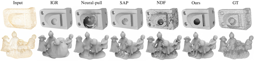
Figure 9: Visual comparisons of surface reconstruction on the SRB dataset.

4.2 Surface Reconstruction for Real Scans

Dataset and metrics. For surface reconstruction of real point cloud scans, we follow SAP to evaluate our methods under the Surface Reconstruction Benchmarks (SRB) [57]. We use Chamfer distance and F-Score with a threshold of 1% for evaluation. Note that the ground truth is dense point clouds.

Comparison. We compare our method with state-of-the-art classic and data-driven surface reconstruction methods in the real scanned SRB dataset, including IGR [20], Point2Mesh [23], Screened Poisson Surface Reconstruction (SPSR) [29], Shape As Points (SAP) [45], Neural-Pull [36] and NDF [12]. The numerical comparison is shown in Tab. 4.3, where we achieve the best accuracy. The visual comparisons in Fig. 9 demonstrate that our method is able to reconstruct a continuous surface with local geometry consistence while other methods struggle to reveal the geometry details. For example, IGR, Neural-Pull and SAP mistakenly mended or failed to reconstruct the hole of the anchor while our method is able to keep the correct geometry.

4.3 Surface Reconstruction for Scenes

Dataset and metrics. To further demonstrate the advantage of our method in surface reconstruction of real scene scans, we follow OnSurf [37] to conduct experiments under the 3D Scene dataset [64]. Note that the 3D Scene dataset is a challenging real-world dataset with complex topology and noisy open surfaces. We uniformly sample 100, 500 and 1000 points per $m^{2}$ at the original scale of scenes as the input and follow OnSurf to sample 1M points on both the reconstructed and the ground truth surfaces. We leverage L1 and L2 Chamfer distance to evaluate the reconstruction quality.

Comparison. We compare our method with the state-of-the-arts scene reconstruction methods ConvONet [46], LIG [26], DeepLS [7], OnSurf [37] and NDF [12]. The numerical comparisons in Tab. 4.3 show that our method significantly outperform the other methods under different point densities. The visual comparisons in Fig. 10 further shows that our reconstructions present more geometry details in complex real scene scans. Note that all the other methods have been trained in a large scale dataset, from which they gain additional prior information. On the contrary, our method does not leverage any additional priors or large scale training datasets, and learns to reconstruct surfaces directly from the raw point cloud, but still yields a non-trivial performance.

Method	100/$m^{2}$		500/$m^{2}$		1000/$m^{2}$
	L2CD	L1CD	L2CD	L1CD	L2CD	L1CD
ConvONet [46]	7.859	0.043	13.192	0.052	14.097	0.052
LIG [20]	6.265	0.049	5.633	0.048	6.190	0.048
DeepLS [7]	3.029	0.044	6.794	0.050	1.607	0.025
NDFPC [12]	0.409	0.012	0.377	0.014	0.561	0.017
NDFmesh	0.452	0.014	0.475	0.016	0.872	0.022
OnSurf [37]	1.154	0.021	0.862	0.020	0.706	0.020
OursPC	0.144	0.010	0.078	0.009	0.072	0.010
Oursmesh	0.187	0.011	0.122	0.010	0.121	0.009

Table 3: Surface Reconstruction under 3D Scene, L2CD$\times$1000.

Method	Chamfer-L1	F-Score
IGR [20]	0.178	75.5
Point2Mesh [23]	0.116	64.8
SPSR [29]	0.232	73.5
SAP [45]	0.076	83.0
Neural-Pull [36]	0.106	79.7
NDFPC [12]	0.185	72.2
NDFmesh	0.238	68.6
OursPC	0.068	90.4
Oursmesh	0.073	84.5

Table 4: Comparisons on SRB.

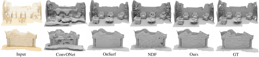
Figure 10: Visual comparison with different methods under 3D Scene. Inputs contains 1k points/$m^{2}$.

4.4 Ablation Study

We conduct ablation studies to justify the effectiveness of each design in our method and the effect of some important parameters. We report the performance in terms of L2-CD under a subset of the ShapeNet Car dataset. By default, all the experimental settings are kept the same as in Sec. 4.1, except for modified part described in each ablation experiment below.

$\times 10^{4}$	NP loss	Exponent	Scratch	Ours
L2CD	0.2381	0.1218	0.1497	0.1112

Table 5: Effect of framework design.

Framework design. We first justify the effectiveness of each design of our framework in Tab. 5. We first directly use the loss proposed in Neural-Pull and find that the performance degenerates dramatically as shown by “NP loss". We also use $g(x)=1-e^{(-x)}$ to replace $g(x)=|x|$ on the last layer of the network for $f$ before output, but found no improvement as shown by “Exponent". We train the second stage from scratch as shown by “Scratch" and prove that an end-to-end training strategy is more effective.

$\times 10^{4}$	1	2	3	4
L2CD	0.1218	0.1112	0.1107	0.1107

Table 6: Effect of stage numbers.

The effect of stage numbers. The number of stages during progressive surface approximation is also a crucial factor in the network training. We report the performance of training our network in different number of stages $St=[1,2,3,4]$ in Tab. 6. We start the training of next stage after the previous one converges. We found that two stages training brings great improvement than training a single stage, and the improvements with 3rd and 4th stages are subtle.

$\times 10^{4}$	0.9	1.0	1.1	1.2
L2CD	0.1133	0.1130	0.1112	0.1131

Table 7: Effect of low confidence range.

The effect of low confidence range. We further explore the range of confidence region sample. Assume $\sigma$ as the range of high confidence region, we use 0.9$\sigma$, 1.0$\sigma$, 1.1$\sigma$ and 1.2$\sigma$ as the range of low confidence region. The results in Tab. 7 show that a too small or too large range will degenerate the performance.

$\times 10^{4}$	643	1283	2563	3203
w/o refine	0.4169	0.1738	0.1294	0.1238
refine	0.1606	0.1174	0.1112	0.1105
Time	3.0 s	21.9 s	162.2 s	307.6 s

Table 8: Ablations on surface extraction.

Surface extraction. We evaluate the effect of mesh refinement and the performance of different 3D grid resolutions. Tab. 8 shows the accuracy and efficiency of different resolutions. We observe that the mesh refinement highly improves the accuracy and higher resolutions leads to better reconstructions at a cost of speed.

5 Conclusion

We propose a novel method to learn continuous UDFs directly from raw point clouds by learning to move 3D queries to reach the approximated surface progressively. Our introduced reconstruction algorithm can extract surfaces directly from the gradient fields of the learned UDFs. Our method does not require ground truth distance values or point normals, and can reconstruct surfaces with arbitrary topology. One limitation of our method is that we use uniformly divided grids to extract surface, which can be improved with a coarse-to-fine paradigm.

Supplementary Material

A Implementation Details

Network design. Our network contains 8 layers of MLP where each layer has 256 nodes. We adopt a skip connection in the fourth layer as employed in DeepSDF [44] and ReLU activation functions in the last two layers of MLP. To make sure the network learns an unsigned distance, we further adopt a non-linear projection $g(x)=|x|$ before the final output.

Training settings. During training, we employ the Adam optimizer with an initial learning rate of 0.001 and a cosine learning rate schedule with 1k warn-up iterations. We start the training of next stage after the previous one converges. In experiment, we found the iteration of 40k, 60k and 70k suitable for the change of stages. Since the 3rd and 4th stages bring little advance as shown in Tab.7 of the main paper, we specify the number of stages as two in practical, so the network has been trained in total 60k iterations. For the surface reconstruction of real scanned complex scenes, we increase the iterations to 300k for a better convergence.

Evaluation settings. For experiments on ShapeNet and 3D Scenes [64], we employ the same evaluation settings as GIFS [59] and OnSurf [37]. We also follow SAP [45] to construct experiments on the SRB dataset [57], however, SAP didn’t provide the evaluation settings of point numbers on the SRB dataset. For a fair comparison, we use the evaluation code provided by SAP and test the reconstructed results provided by the author of SAP under different evaluation settings where we found that sampling 50k points on the reconstructed shapes and 150k points on the ground truth shapes can completely reproduce the results of SAP.

B Proofs

Assumption: Given a raw point cloud which is a discrete representation of the surface, we have made a reasonable assumption: the closer the query location is to the given point cloud, the smaller the error of searching the target point on the given point cloud.

In the task of surface reconstruction, one of the key properties is local planarity, that is, the surface can be approximated by tangent plane with infinite accuracy. In graphics, the common form of expressing surfaces is polygon mesh. To complete our proof, we provide a few necessary definitions,

Definition 1. Polygon mesh is a collection of vertices, edges and faces that defines the surface of 3D shape $S=(V,F)$. Vertices $V=\left\{v_{1},\ldots,v_{w}\right\}$ determine the position of the faces in 3D space. The edges represent the connection between two vertices, thus a closed set of edges forming the faces $F=\left\{f_{1},\ldots,f_{e}\right\}$.

Definition 2. Given a point cloud $P=\{p_{i},i\in[1,N]\}$, its ground truth surface model $S=(V,F)$ consists of vertices $V=\left\{v_{1},\ldots,v_{w}\right\}$ and faces $F=\left\{f_{1},\ldots,f_{e}\right\}$. Assume that given a set of query points $Q=\{q_{i},i\in[1,M]\}$, the nearest point of query point $q_{i}$ on the model $S=(V,F)$ is $g_{i}$, and $g_{i}$ must be on one of the faces $F$. We define the meaning of error of searching the target point on the given point cloud, $E(S,P,Q)=\sum_{i\in[1,M]}\min_{j\in[1,N]}\left\|g_{i}-p_{j}\right\|_{2}$.

Review our strategy for sampling query points: We sample $m$ queries around each point $p_{i}$ on $P$. A Gaussian function $\mathcal{N}(\mu,\sigma^{2})$ is adopt to calculate the sampling probability for generaing query location $q_{\sigma}^{i,j},j\in[1,m]$, where $\mu=p_{i}$. Suppose we collect two sets of query points $Q_{\sigma_{1}}=\{q_{\sigma_{1}}^{i,j}\mid i\in[1,N],j\in[1,m]\}$ and $Q_{\sigma_{2}}=\{q_{\sigma_{2}}^{i,j}\mid i\in[1,N],j\in[1,m]\}$, where $\sigma_{1}$ and $\sigma_{2}$ are standard deviations of the sampled Gaussian function.

Theorem 1. Given a point cloud $P=\{p_{i},i\in[1,N]\}$ and its ground truth surface model $S=(V,F)$. Assume two sets of query points $Q_{\sigma_{1}}$ and $Q_{\sigma_{2}}$ are sampled, where $\sigma_{1}>\sigma_{2}$ , then $E(S,P,Q_{\sigma_{1}})>E(S,P,Q_{\sigma_{2}})$.

Proof 1. Queries $q_{\sigma}^{i,j},j\in[1,m]$ are sampled around point $p_{i}$ of the given point cloud $P$. Assume that the nearest surface point on the model $S=(V,F)$ to the query point $q_{\sigma}^{i,j}$ is $g_{\sigma}^{i,j}$, where $g_{\sigma}^{i,j}$ on the face $f_{\sigma}^{i,j,k}$. The point $p_{i}$ must be on one of the faces $F$, assuming that this face is $f_{u}$. Let $Q_{\sigma_{1}}^{i}=\left\{q_{\sigma_{1}}^{i,j}\mid j\in[1,m]\right\}$,$Q_{\sigma_{2}}^{i}=\left\{q_{\sigma_{2}}^{i,j}\mid j\in[1,m]\right\}$, where $\sigma_{1}>\sigma_{2}$. We decompose $Q_{\sigma_{1}}^{i}$ and $Q_{\sigma_{2}}^{i}$ to the two sides, $Q_{\sigma_{1},i}^{+}=\left\{{q_{\sigma_{1}}^{i,j}\mid f_{\sigma_{1}}^{i,j,k}=f_{u}}\right\}$,$Q_{\sigma_{2},i}^{+}=\left\{{q_{\sigma_{2}}^{i,j}\mid f_{\sigma_{2}}^{i,j,k}=f_{u}}\right\}$, and $Q_{\sigma_{1},i}^{-}=\left\{{q_{\sigma_{1}}^{i,j}\mid f_{\sigma_{1}}^{i,j,k}\neq f_{u}}\right\}$, $Q_{\sigma_{2},i}^{-}=\left\{{q_{\sigma_{2}}^{i,j}\mid f_{\sigma_{2}}^{i,j,k}\neq f_{u}}\right\}$. Therefore $E(S,P,Q_{\sigma_{1}}^{i})=E(S,P,Q_{\sigma_{1},i}^{+})+E(S,P,Q_{\sigma_{1},i}^{-})$, $E(S,P,Q_{\sigma_{2}}^{i})=E(S,P,Q_{\sigma_{2},i}^{+})+E(S,P,Q_{\sigma_{2},i}^{-})$. Since the sampling probability is calculated based on Gaussian function, that is defined by density function $\mu(q)$, assuming that $f_{u}=n^{T}x+d$,

$$\begin{split}E(S,P,Q_{\sigma_{1},i}^{+})=&\int||g_{\sigma_{1}}^{i,j}-p_{i}\|_{2}\mu(q_{\sigma_{1}}^{i,j})d(q_{\sigma_{1}}^{i,j})\\ =&\sum_{j\in[1,m]}||q_{\sigma_{1}}^{i,j}-\frac{q_{\sigma_{1}}^{i,j}\cdot n^{T}+d}{n^{T}\cdot n^{T}}\cdot n^{T}-p_{i}\|_{2}\frac{1}{\sqrt{(2\pi)^{3}\sigma_{1}|I|}}e^{-\frac{1}{2}(q_{\sigma_{1}}^{i,j}-p_{i})^{T}\sigma_{1}I(q_{\sigma_{1}}^{i,j}-p_{i})}\end{split}$$ (4)

Since $E(S,P,Q_{\sigma_{1},i}^{+})$ will decrease with decreasing $\sigma_{1}$, then we get $E(S,P,Q_{\sigma_{1},i}^{+})>E(S,P,Q_{\sigma_{2},i}^{+})$.

The geometric distribution of $f_{\sigma}^{i,j,k}$ appearing around $f_{u}$ can be regarded as randomly distributed, the $E(S,P,Q_{\sigma,i}^{-})$ is also randomly distributed and independent of the density function, so that in a statistical sense, $E(S,P,Q_{\sigma{1},i}^{-})=E(S,P,Q_{\sigma_{2},i}^{-})$. Then we get $E(S,P,Q_{\sigma_{1},i})>E(S,P,Q_{\sigma_{2},i})$. The case of arbitrary other $Q_{\sigma_{1}}^{j}$ and $Q_{\sigma_{2}}^{j}$ proven similarly. So we proof $E(S,P,Q_{\sigma_{1}})>E(S,P,Q_{\sigma_{2}})$.

C Additional Experiments

The effect of training iterations. We further test the effect of training iterations of the first and second stage. Since we use an end-to-end training strategy, we set a relatively small number of training iterations for the second stage. In experiments, we set the numbers of iteration in the first stage to 30k, 40k and 50k, and the second stage to 15k, 20k and 25k. For testing the effect of the iteration numbers in the first stage, we set the iteration numbers of second stage to the default 20k, and the iteration numbers of first stage is set to the default 40k while testing the second stage. The results in Tab. 9 show that too few training iterations will lead to an under fitting problem and too many training iterations will result in network degradation.

Stage1	30k	40k	50k
Chamfer-L2	0.1158	0.1112	0.1137
Stage2	15k	20k	25k
Chamfer-L2	0.1125	0.1112	0.1133

Table 9: Effect on training iterations of different stages.

Efficiency comparison on field learning. We make a comparison with Neural-Pull [36], IGR [20], Point2mesh [23] on the computational cost of optimizing for a single point cloud in Table 10. The results show that our proposed method converges faster than all the baselines with fewer memory requirements.

Methods	Neural-Pull	IGR	Point2mesh	Ours
Time (s)	1150	1212	4028	667
Memory (GB)	2.2	6.1	5.2	2.0

Table 10: Efficiency comparison on field learning.

Efficiency comparison on mesh extraction. We further evaluate the efficiency of our method. The comparison is shown in Tab. 11. For reproducing the mesh generation process of NDF [12], we use the default 1$\times 10^{6}$ points and the parameters provided by NDF to generate a mesh with ball-pivoting-algorithm (BPA) [3]. It’s clear that our method achieves a tremendous advantage over NDF even with a relatively high resolution (e.g.256³). The reason is that our method allows a straightforward surface extracting from the learned UDFs while the ball-pivoting-algorithm used by NDF requires a lot of calculations for neighbour searching and normal estimation.

Method	NDF [12]	Ours 643	Ours 1283	Ours 2563	Ours 3203
Time	2080.7 s	3.0 s	21.9 s	162.2 s	307.6 s

Table 11: Efficiency comparison of surface generation.

The complete comparison under 3D Scene dataset. We also provide the complete comparison under all the five scenes of the 3D Scene dataset [64]. The results is shown in Tab. 12. We provide a comprehensive comparison with NDF by comparing both the generated point cloud (*_PC) and the generated mesh (*_mesh). We use L1 and L2 chamfer distance (L2CD, L1CD) as evaluation metrics.

		Burghers		Lounge		Copyroom		Stonewall		Totempole
		L2CD	L1CD	L2CD	L1CD	L2CD	L1CD	L2CD	L1CD	L2CD	L1CD
100/$m^{2}$	COcc [46]	8.904	0.040	6.979	0.041	6.78	0.041	12.22	0.051	4.412	0.041
	LIG [26]	3.112	0.044	9.128	0.054	4.363	0.039	5.143	0.046	9.58	0.062
	DeepLS [7]	3.111	0.050	3.894	0.056	1.498	0.033	2.427	0.038	4.214	0.043
	NDFPC [12]	0.320	0.012	0.417	0.013	0.291	0.012	0.252	0.010	0.767	0.015
	NDFmesh [12]	0.463	0.014	0.484	0.015	0.439	0.015	0.248	0.011	0.624	0.014
	OnSurf [37]	0.544	0.018	0.435	0.013	0.434	0.017	0.371	0.016	3.986	0.040
	OursPC	0.121	0.010	0.277	0.013	0.150	0.010	0.079	0.008	0.090	0.008
	Oursmesh	0.212	0.011	0.245	0.011	0.214	0.012	0.118	0.009	0.145	0.009
500/$m^{2}$	COcc [46]	26.97	0.081	9.044	0.046	10.08	0.046	17.70	0.063	2.165	0.024
	LIG [26]	3.080	0.046	6.729	0.052	4.058	0.038	4.919	0.043	9.38	0.062
	DeepLS [7]	0.714	0.020	10.88	0.077	0.552	0.015	0.673	0.018	21.15	0.122
	NDFPC [12]	0.304	0.014	0.261	0.011	0.162	0.010	0.239	0.012	0.919	0.021
	NDFmesh [12]	0.546	0.018	0.314	0.012	0.242	0.012	0.226	0.012	1.049	0.025
	OnSurf [37]	0.609	0.018	0.529	0.013	0.483	0.014	0.666	0.013	2.025	0.041
	OursPC	0.072	0.008	0.146	0.011	0.072	0.008	0.038	0.007	0.064	0.008
	Oursmesh	0.192	0.011	0.099	0.009	0.120	0.009	0.069	0.008	0.131	0.010
1000/$m^{2}$	COcc [46]	27.46	0.079	9.54	0.046	10.97	0.045	20.46	0.069	2.054	0.021
	LIG [26]	3.055	0.045	9.672	0.056	3.61	0.036	5.032	0.042	9.58	0.062
	DeepLS [7]	0.401	0.017	6.103	0.053	0.609	0.021	0.320	0.015	0.601	0.017
	NDFPC [12]	0.575	0.019	0.303	0.012	0.186	0.011	0.407	0.016	1.333	0.026
	NDFmesh [12]	1.168	0.027	0.393	0.014	0.269	0.013	0.509	0.019	2.020	0.036
	OnSurf [37]	1.339	0.031	0.432	0.014	0.405	0.014	0.266	0.014	1.089	0.029
	OursPC	0.087	0.010	0.057	0.009	0.083	0.010	0.043	0.007	0.086	0.010
	Oursmesh	0.191	0.010	0.092	0.008	0.113	0.009	0.066	0.007	0.139	0.009

Table 12: Surface reconstruction for point clouds under 3D Scene. L2CD$\times 1000$.

D Additional Visualizations

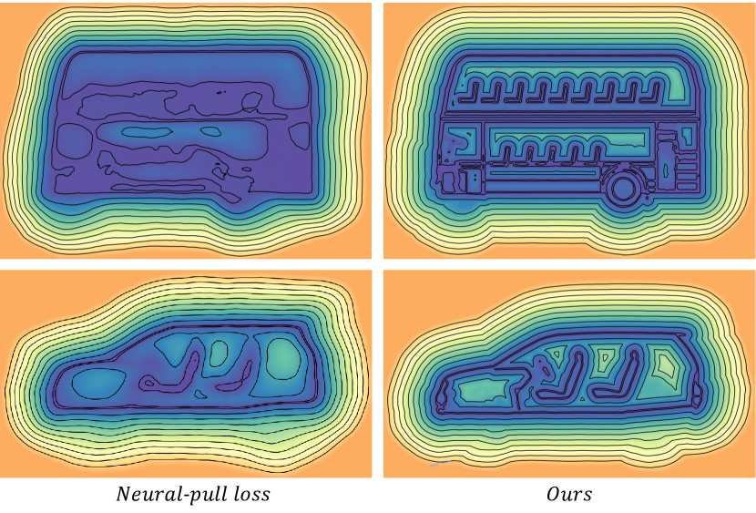
Figure 11: Visualizations of the unsigned distance field. The darker the color, the closer it is to the approximated surface. For a clear contrast, we set the color of the space far away from the approximated surface to orange.

Visualizations of the unsigned distance field. To further evaluate the effectiveness of our consistency-aware field learning, we visualize the learned unsigned distance fields with Neural-Pull [36] loss in Eq. (2) of our submission and our field consistency loss in Eq. (3) of our submission. Fig. 11 shows the visual comparison under two different shapes with complex inner structures. For the storey bus, training with the loss proposed by Neural-Pull fails to handle the rich structures, thus leads to a chaotic distance field where no details were kept. On the contrary, our proposed consistency-aware learning can build a consistent distance field where the detailed structures are well preserved. It’s clear that our method learns a highly continuous unsigned distance field and has the ability to keep the field around complex structures correct (e.g. the seats, tires and stairs), which also helps to extract a high fidelity surface.

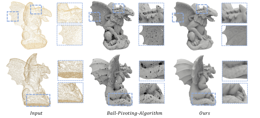
Figure 12: Visual comparison with ball-pivoting-algorithm.

Visual comparison with ball-pivoting-algorithm. To further explore the advantage of our straightforward surface extraction algorithm, we use the same setting as NDF [12] to adopt ball-pivoting-algorithm (BPA) [3] to extract mesh from our generated point cloud and make a comparison with the mesh extracted using our method as shown in Fig. 12. Even with a carefully selected threshold, the mesh generated by BPA is still far from smooth and has a number of holes, and also fails to retain the detailed geometric information. On the contrary, our method allows to extract surfaces directly from the learned UDFs, thus is able to reconstruct a continuous and high-fidelity mesh where the geometry details is well preserved.

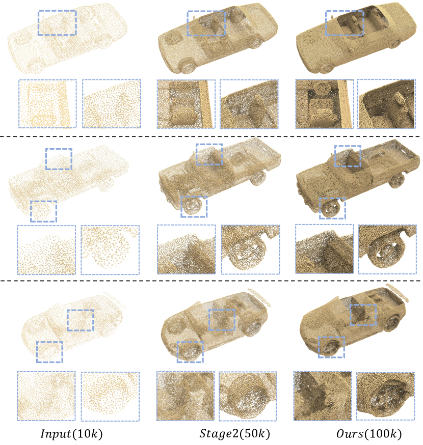
Figure 13: Visualizations of our generated intermediate and final point clouds.

Visualizations of our generated intermediate and final point clouds. As shown in Fig. 13, we provide the visualizations of the raw input point cloud as ‘Input’ and the intermediate point cloud updated by the well-moved queries which serves as the target point cloud at the second stage, as shown by ‘Stage2’. We also provide the generated dense point cloud by moving the queries to the approximated surface using Eq. (1) in our submission as shown by ‘Ours’. The raw input point cloud is highly discrete and fails to provide detailed supervision for surface reconstruction. On the contrary, the intermediate point cloud updated by the well-moved queries shows great uniformity and continuity, thus can provide the supervision of fine geometries such as the detailed steering wheel and tires of the car. The quantitative comparison of using the raw input point cloud and the intermediate point cloud as target for surface reconstruction is shown in Tab. 6 of our submission, where leveraging the intermediate point cloud as target can achieve $10\%$ improvement over leveraging the raw input point cloud. Furthermore, due to our progressive surface approximation strategy, our generated dense point cloud can maintain uniformity and keep the detailed geometric.

Visualizations of meshes extracted with different settings. We provide the visualizations of the extracted surfaces with different resolutions as shown in Fig. 14. It shows that a higher resolution leads to a more detailed reconstruction. Moreover, our designed mesh refinement operation brings great improvement in surface smoothness and local details due to the accurate unsigned distance values predicted by the neural network.

More visualization comparisons. We provide more visual comparisons under Surface Reconstruction Benchmark (SRB) dataset [57] in Fig. 15 and MGD dataset [4] in Fig. 16, respectively.

E Future works.

We consider two potential future works of our method. First, although the experiments under real scanned shapes and scenes proved the ability of our proposed method in handling noises with unknown distributions, we think it’s an interesting future work to extend our method for reconstructing surfaces from high-noisy point clouds in an unsupervised way. Second, by transferring the sliding window strategy [7, 47] to our method, it’s exciting to see the ability of extending our method for representing large scale data.

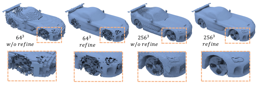
Figure 14: Visualizations of extracted mesh with different settings.

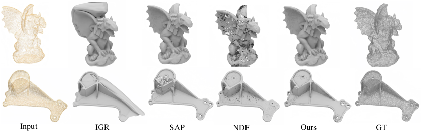
Figure 15: More visualizations under SRB dataset.

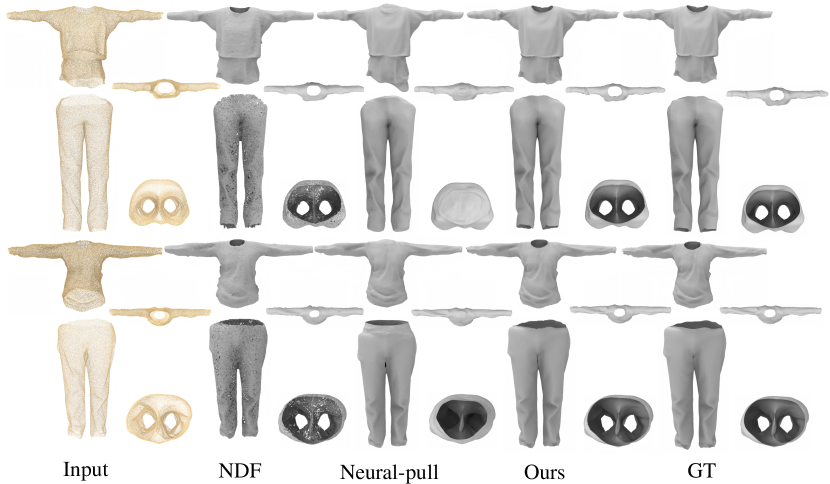
Figure 16: More visualizations under MGD dataset.

References

- [1] Matan Atzmon and Yaron Lipman. SAL: Sign agnostic learning of shapes from raw data. In Proceedings of the IEEE/CVF Conference on Computer Vision and Pattern Recognition, pages 2565–2574, 2020.
- [2] Matan Atzmon and Yaron Lipman. SALD: Sign agnostic learning with derivatives. In International Conference on Learning Representations, 2020.
- [3] Fausto Bernardini, Joshua Mittleman, Holly Rushmeier, Cláudio Silva, and Gabriel Taubin. The ball-pivoting algorithm for surface reconstruction. IEEE Transactions on Visualization and Computer Graphics, 5(4):349–359, 1999.
- [4] Bharat Lal Bhatnagar, Garvita Tiwari, Christian Theobalt, and Gerard Pons-Moll. Multi-garment net: Learning to dress 3D people from images. In Proceedings of the IEEE/CVF International Conference on Computer Vision, pages 5420–5430, 2019.
- [5] John Bibby. Axiomatisations of the average and a further generalisation of monotonic sequences. Glasgow Mathematical Journal, 15(1):63–65, 1974.
- [6] Alexandre Boulch and Renaud Marlet. POCO: Point convolution for surface reconstruction. In Proceedings of the IEEE/CVF Conference on Computer Vision and Pattern Recognition, pages 6302–6314, 2022.
- [7] Rohan Chabra, Jan E Lenssen, Eddy Ilg, Tanner Schmidt, Julian Straub, Steven Lovegrove, and Richard Newcombe. Deep local shapes: Learning local sdf priors for detailed 3D reconstruction. In European Conference on Computer Vision, pages 608–625. Springer, 2020.
- [8] Chao Chen, Zhizhong Han, Yu-Shen Liu, and Matthias Zwicker. Unsupervised learning of fine structure generation for 3D point clouds by 2D projections matching. In Proceedings of the ieee/cvf international conference on computer vision, pages 12466–12477, 2021.
- [9] Chao Chen, Yu-Shen Liu, and Zhizhong Han. Latent partition implicit with surface codes for 3D representation. In European Conference on Computer Vision (ECCV), 2022.
- [10] Zhiqin Chen and Hao Zhang. Learning implicit fields for generative shape modeling. In Proceedings of the IEEE/CVF Conference on Computer Vision and Pattern Recognition, pages 5939–5948, 2019.
- [11] Julian Chibane, Thiemo Alldieck, and Gerard Pons-Moll. Implicit functions in feature space for 3D shape reconstruction and completion. In Proceedings of the IEEE/CVF Conference on Computer Vision and Pattern Recognition, pages 6970–6981, 2020.
- [12] Julian Chibane, Gerard Pons-Moll, et al. Neural unsigned distance fields for implicit function learning. Advances in Neural Information Processing Systems, 33:21638–21652, 2020.
- [13] François Darmon, Bénédicte Bascle, Jean-Clément Devaux, Pascal Monasse, and Mathieu Aubry. Improving neural implicit surfaces geometry with patch warping. In Proceedings of the IEEE/CVF Conference on Computer Vision and Pattern Recognition, pages 6260–6269, 2022.
- [14] Yueqi Duan, Haidong Zhu, He Wang, Li Yi, Ram Nevatia, and Leonidas J Guibas. Curriculum deepsdf. In European Conference on Computer Vision, pages 51–67. Springer, 2020.
- [15] Herbert Edelsbrunner and Ernst P Mücke. Three-dimensional alpha shapes. ACM Transactions on Graphics (TOG), 13(1):43–72, 1994.
- [16] Philipp Erler, Paul Guerrero, Stefan Ohrhallinger, Niloy J Mitra, and Michael Wimmer. Points2surf learning implicit surfaces from point clouds. In European Conference on Computer Vision, pages 108–124. Springer, 2020.
- [17] Qiancheng Fu, Qingshan Xu, Yew-Soon Ong, and Wenbing Tao. Geo-Neus: Geometry-consistent neural implicit surfaces learning for multi-view reconstruction. arXiv preprint arXiv:2205.15848, 2022.
- [18] Kyle Genova, Forrester Cole, Avneesh Sud, Aaron Sarna, and Thomas Funkhouser. Local deep implicit functions for 3D shape. In Proceedings of the IEEE/CVF Conference on Computer Vision and Pattern Recognition, pages 4857–4866, 2020.
- [19] Kyle Genova, Forrester Cole, Daniel Vlasic, Aaron Sarna, William T Freeman, and Thomas Funkhouser. Learning shape templates with structured implicit functions. In Proceedings of the IEEE/CVF International Conference on Computer Vision, pages 7154–7164, 2019.
- [20] Amos Gropp, Lior Yariv, Niv Haim, Matan Atzmon, and Yaron Lipman. Implicit geometric regularization for learning shapes. In International Conference on Machine Learning, pages 3789–3799. PMLR, 2020.
- [21] Benoit Guillard, Federico Stella, and Pascal Fua. Meshudf: Fast and differentiable meshing of unsigned distance field networks. arXiv preprint arXiv:2111.14549, 2021.
- [22] Zhizhong Han, Baorui Ma, Yu-Shen Liu, and Matthias Zwicker. Reconstructing 3D shapes from multiple sketches using direct shape optimization. IEEE Transactions on Image Processing, 29:8721–8734, 2020.
- [23] Rana Hanocka, Gal Metzer, Raja Giryes, and Daniel Cohen-Or. Point2mesh: a self-prior for deformable meshes. ACM Transactions on Graphics (TOG), 39(4):126–1, 2020.
- [24] Tao Hu, Zhizhong Han, and Matthias Zwicker. 3D shape completion with multi-view consistent inference. In Proceedings of the AAAI Conference on Artificial Intelligence, volume 34, pages 10997–11004, 2020.
- [25] Meng Jia and Matthew Kyan. Learning occupancy function from point clouds for surface reconstruction. arXiv preprint arXiv:2010.11378, 2020.
- [26] Chiyu Jiang, Avneesh Sud, Ameesh Makadia, Jingwei Huang, Matthias Nießner, Thomas Funkhouser, et al. Local implicit grid representations for 3D scenes. In Proceedings of the IEEE/CVF Conference on Computer Vision and Pattern Recognition, pages 6001–6010, 2020.
- [27] Yue Jiang, Dantong Ji, Zhizhong Han, and Matthias Zwicker. SDFDiff: Differentiable rendering of signed distance fields for 3D shape optimization. In IEEE Conference on Computer Vision and Pattern Recognition, 2020.
- [28] Michael Kazhdan, Matthew Bolitho, and Hugues Hoppe. Poisson surface reconstruction. In Proceedings of the fourth Eurographics Symposium on Geometry Processing, volume 7, 2006.
- [29] Michael Kazhdan and Hugues Hoppe. Screened poisson surface reconstruction. ACM Transactions on Graphics (ToG), 32(3):1–13, 2013.
- [30] Tianyang Li, Xin Wen, Yu-Shen Liu, Hua Su, and Zhizhong Han. Learning deep implicit functions for 3D shapes with dynamic code clouds. In Proceedings of the IEEE/CVF Conference on Computer Vision and Pattern Recognition, pages 12840–12850, 2022.
- [31] David B Lindell, Dave Van Veen, Jeong Joon Park, and Gordon Wetzstein. Bacon: Band-limited coordinate networks for multiscale scene representation. In Proceedings of the IEEE/CVF Conference on Computer Vision and Pattern Recognition, pages 16252–16262, 2022.
- [32] Shi-Lin Liu, Hao-Xiang Guo, Hao Pan, Peng-Shuai Wang, Xin Tong, and Yang Liu. Deep implicit moving least-squares functions for 3D reconstruction. In Proceedings of the IEEE/CVF Conference on Computer Vision and Pattern Recognition, pages 1788–1797, 2021.
- [33] Xinhai Liu, Xinchen Liu, Yu-Shen Liu, and Zhizhong Han. Spu-net: Self-supervised point cloud upsampling by coarse-to-fine reconstruction with self-projection optimization. IEEE Transactions on Image Processing, 31:4213–4226, 2022.
- [34] Sandro Lombardi, Martin R Oswald, and Marc Pollefeys. Scalable point cloud-based reconstruction with local implicit functions. In 2020 International Conference on 3D Vision (3DV), pages 997–1007. IEEE, 2020.
- [35] William E Lorensen and Harvey E Cline. Marching cubes: A high resolution 3D surface construction algorithm. ACM Siggraph Computer Graphics, 21(4):163–169, 1987.
- [36] Baorui Ma, Zhizhong Han, Yu-Shen Liu, and Matthias Zwicker. Neural-Pull: Learning signed distance function from point clouds by learning to pull space onto surface. In International Conference on Machine Learning, pages 7246–7257. PMLR, 2021.
- [37] Baorui Ma, Yu-Shen Liu, and Zhizhong Han. Reconstructing surfaces for sparse point clouds with on-surface priors. In Proceedings of the IEEE/CVF Conference on Computer Vision and Pattern Recognition, 2022.
- [38] Baorui Ma, Yu-Shen Liu, Matthias Zwicker, and Zhizhong Han. Surface reconstruction from point clouds by learning predictive context priors. In Proceedings of the IEEE/CVF Conference on Computer Vision and Pattern Recognition, 2022.
- [39] Julien NP Martel, David B Lindell, Connor Z Lin, Eric R Chan, Marco Monteiro, and Gordon Wetzstein. Acorn: adaptive coordinate networks for neural scene representation. ACM Transactions on Graphics (TOG), 40(4):1–13, 2021.
- [40] Lars Mescheder, Michael Oechsle, Michael Niemeyer, Sebastian Nowozin, and Andreas Geiger. Occupancy networks: Learning 3D reconstruction in function space. In Proceedings of the IEEE/CVF Conference on Computer Vision and Pattern Recognition, pages 4460–4470, 2019.
- [41] Zhenxing Mi, Yiming Luo, and Wenbing Tao. Ssrnet: Scalable 3D surface reconstruction network. In Proceedings of the IEEE/CVF Conference on Computer Vision and Pattern Recognition, pages 970–979, 2020.
- [42] Mateusz Michalkiewicz, Jhony K Pontes, Dominic Jack, Mahsa Baktashmotlagh, and Anders Eriksson. Deep level sets: Implicit surface representations for 3D shape inference. arXiv preprint arXiv:1901.06802, 2019.
- [43] Michael Oechsle, Songyou Peng, and Andreas Geiger. Unisurf: Unifying neural implicit surfaces and radiance fields for multi-view reconstruction. In Proceedings of the IEEE/CVF International Conference on Computer Vision, pages 5589–5599, 2021.
- [44] Jeong Joon Park, Peter Florence, Julian Straub, Richard Newcombe, and Steven Lovegrove. Deepsdf: Learning continuous signed distance functions for shape representation. In Proceedings of the IEEE/CVF Conference on Computer Vision and Pattern Recognition, pages 165–174, 2019.
- [45] Songyou Peng, Chiyu Jiang, Yiyi Liao, Michael Niemeyer, Marc Pollefeys, and Andreas Geiger. Shape as points: A differentiable poisson solver. Advances in Neural Information Processing Systems, 34, 2021.
- [46] Songyou Peng, Michael Niemeyer, Lars Mescheder, Marc Pollefeys, and Andreas Geiger. Convolutional occupancy networks. In European Conference on Computer Vision, pages 523–540. Springer, 2020.
- [47] Matthew Tancik, Vincent Casser, Xinchen Yan, Sabeek Pradhan, Ben Mildenhall, Pratul P Srinivasan, Jonathan T Barron, and Henrik Kretzschmar. Block-nerf: Scalable large scene neural view synthesis. In Proceedings of the IEEE/CVF Conference on Computer Vision and Pattern Recognition, pages 8248–8258, 2022.
- [48] Edgar Tretschk, Ayush Tewari, Vladislav Golyanik, Michael Zollhöfer, Carsten Stoll, and Christian Theobalt. Patchnets: Patch-based generalizable deep implicit 3D shape representations. In European Conference on Computer Vision, pages 293–309. Springer, 2020.
- [49] Rahul Venkatesh, Tejan Karmali, Sarthak Sharma, Aurobrata Ghosh, R Venkatesh Babu, László A Jeni, and Maneesh Singh. Deep implicit surface point prediction networks. In Proceedings of the IEEE/CVF International Conference on Computer Vision, pages 12653–12662, 2021.
- [50] Bing Wang, Zhengdi Yu, Bo Yang, Jie Qin, Toby Breckon, Ling Shao, Niki Trigoni, and Andrew Markham. Rangeudf: Semantic surface reconstruction from 3D point clouds. arXiv preprint arXiv:2204.09138, 2022.
- [51] Peng Wang, Lingjie Liu, Yuan Liu, Christian Theobalt, Taku Komura, and Wenping Wang. Neus: Learning neural implicit surfaces by volume rendering for multi-view reconstruction. Advances in Neural Information Processing Systems, 34:27171–27183, 2021.
- [52] Yiqun Wang, Ivan Skorokhodov, and Peter Wonka. Improved surface reconstruction using high-frequency details. arXiv preprint arXiv:2206.07850, 2022.
- [53] Xin Wen, Zhizhong Han, Yan-Pei Cao, Pengfei Wan, Wen Zheng, and Yu-Shen Liu. Cycle4completion: Unpaired point cloud completion using cycle transformation with missing region coding. In Proceedings of the IEEE/CVF conference on computer vision and pattern recognition, pages 13080–13089, 2021.
- [54] Xin Wen, Peng Xiang, Zhizhong Han, Yan-Pei Cao, Pengfei Wan, Wen Zheng, and Yu-Shen Liu. Pmp-net: Point cloud completion by learning multi-step point moving paths. In Proceedings of the IEEE/CVF Conference on Computer Vision and Pattern Recognition, pages 7443–7452, 2021.
- [55] Xin Wen, Peng Xiang, Zhizhong Han, Yan-Pei Cao, Pengfei Wan, Wen Zheng, and Yu-Shen Liu. Pmp-net++: Point cloud completion by transformer-enhanced multi-step point moving paths. IEEE Transactions on Pattern Analysis and Machine Intelligence, 2022.
- [56] Xin Wen, Junsheng Zhou, Yu-Shen Liu, Hua Su, Zhen Dong, and Zhizhong Han. 3D shape reconstruction from 2D images with disentangled attribute flow. In Proceedings of the IEEE/CVF Conference on Computer Vision and Pattern Recognition, pages 3803–3813, 2022.
- [57] Francis Williams, Teseo Schneider, Claudio Silva, Denis Zorin, Joan Bruna, and Daniele Panozzo. Deep geometric prior for surface reconstruction. In Proceedings of the IEEE/CVF Conference on Computer Vision and Pattern Recognition, pages 10130–10139, 2019.
- [58] Peng Xiang, Xin Wen, Yu-Shen Liu, Yan-Pei Cao, Pengfei Wan, Wen Zheng, and Zhizhong Han. Snowflakenet: Point cloud completion by snowflake point deconvolution with skip-transformer. In Proceedings of the IEEE/CVF international conference on computer vision, pages 5499–5509, 2021.
- [59] Jianglong Ye, Yuntao Chen, Naiyan Wang, and Xiaolong Wang. GIFS: Neural implicit function for general shape representation. Proceedings of the IEEE/CVF Conference on Computer Vision and Pattern Recognition, 2022.
- [60] Wang Yifan, Shihao Wu, Cengiz Oztireli, and Olga Sorkine-Hornung. Iso-points: Optimizing neural implicit surfaces with hybrid representations. In Proceedings of the IEEE/CVF Conference on Computer Vision and Pattern Recognition, pages 374–383, 2021.
- [61] Wenyuan Zhang, Ruofan Xing, Yunfan Zeng, Yu-Shen Liu, Kanle Shi, and Zhizhong Han. Fast learning radiance fields by shooting much fewer rays. arXiv preprint arXiv:2208.06821, 2022.
- [62] Fang Zhao, Wenhao Wang, Shengcai Liao, and Ling Shao. Learning anchored unsigned distance functions with gradient direction alignment for single-view garment reconstruction. In Proceedings of the IEEE/CVF International Conference on Computer Vision, pages 12674–12683, 2021.
- [63] Junsheng Zhou, Xin Wen, Baorui Ma, Yu-Shen Liu, Yue Gao, Yi Fang, and Zhizhong Han. Self-supervised point cloud representation learning with occlusion auto-encoder. arXiv preprint arXiv:2203.14084, 2022.
- [64] Qian-Yi Zhou and Vladlen Koltun. Dense scene reconstruction with points of interest. ACM Transactions on Graphics (ToG), 32(4):1–8, 2013.