A correlated pseudo-marginal approach to doubly intractable problems

Abstract

Doubly intractable models are encountered in a number of fields, e.g. social networks, ecology and epidemiology. Inference for such models requires the evaluation of a likelihood function, whose normalising function depends on the model parameters and is typically computationally intractable. The normalising constant of the posterior distribution and the additional normalising function of the likelihood function result in a so-called doubly intractable posterior, for which it is difficult to directly apply Markov chain Monte Carlo (MCMC) methods. We propose a signed pseudo-marginal Metropolis-Hastings (PMMH) algorithm with an unbiased block-Poisson estimator to sample from the posterior distribution of doubly intractable models. As the estimator can be negative, the algorithm targets the absolute value of the estimated posterior and uses an importance sampling correction to ensure simulation consistent estimates of the posterior mean of any function. The advantages of our estimator over previous approaches are that its form is ideal for correlated pseudo-marginal methods which are well known to dramatically increase sampling efficiency. Moreover, we develop analytically derived heuristic guidelines for optimally tuning the hyperparameters of the estimator. We demonstrate the algorithm on the Ising model and a Kent distribution model for spherical data.

Keywords Block-Poisson estimator, Ising model, Spherical data.

1 Introduction

Markov chain Monte Carlo (MCMC) methods (see, e.g., Brooks et al.,, 2011, for an overview) sample from the posterior distribution without evaluating the normalising constant, also known as the marginal likelihood. However, in some settings, the likelihood function itself contains an additional normalising constant that depends on the model parameters and the resulting so-called doubly intractable posterior distribution falls outside the standard MCMC framework. To distinguish these normalisation quantities, we refer to the first as a normalising constant and the latter as a normalising function. Many well-known models have doubly intractable posteriors, such as the exponential random graph models for social networks (Hunter and Handcock,, 2006) and non-Gaussian Markov random field models in spatial statistics, including the Ising model and its variants (Lenz,, 1920; Ising,, 1925; Hughes et al.,, 2011).

Several algorithms are available to tackle the doubly intractable problem in Bayesian statistics; see Park and Haran, (2018) for a review. These algorithms are classified into two main categories, with some overlap between them. The first category of methods introduce cleverly chosen auxiliary variables that cancel the normalising function when carrying out the MCMC sampling and standard MCMC such as the Metropolis-Hastings (MH) algorithm (Metropolis et al.,, 1953; Hastings,, 1970) can thus be applied. This approach is model dependent and cannot always be applied. The second category of methods, which applies more generally, approximates the likelihood function (including the normalising function) and substitutes the approximation in place of the exact likelihood in the estimation procedure. The pseudo-marginal (PM) method (Beaumont,, 2003; Andrieu and Roberts,, 2009) is often used when a positive and unbiased estimator of the likelihood is available through Monte Carlo simulation. However, in some problems, including doubly intractable models, forming an unbiased estimator that is almost surely positive is prohibitively expensive (Jacob and Thiery,, 2015). The so-called Russian roulette (RR) estimator (Lyne et al.,, 2015) is an example of a method that can be used to unbiasedly estimate the likelihood function in doubly intractable models, although the estimate is not necessarily positive.

We propose a method for exact inference on posterior expectations in doubly intractable problems based on the approach in Lyne et al., (2015), where an unbiased, but not necessarily positive, estimator of the likelihood function is used. The algorithm targets a posterior density that uses the absolute value of the likelihood, resulting in iterates from a perturbed target density. We follow Lyne et al., (2015) and reweight the samples from the perturbed target density using importance sampling to obtain simulation-consistent estimates of the expectation of any function of the parameters with respect to the true posterior density. While our method does not sample from the target of interest, we refer to it as exact due to its simulation-consistent property.

Our main contribution is to explore the use of the block-Poisson (BP) estimator (Quiroz et al.,, 2021) in the context of estimating doubly intractable models using the signed PMMH approach. Our method provides the following advantages over the Russian roulette method. First, the BP estimator has a much simpler structure and is more computationally efficient. Second, the block form of our estimator makes it possible to correlate the estimators of the doubly intractable posterior at the current and proposed draws in the MH algorithm. Introducing such correlation dramatically improves the efficiency of PM algorithms (Tran et al.,, 2016; Deligiannidis et al.,, 2018). Finally, under simplifying assumptions, some statistical properties of the logarithm of the absolute value of our estimator are derived and used to obtain heuristic guidelines to optimally tune the hyperparameters of the estimator. We demonstrate empirically that our method outperforms Lyne et al., (2015) when estimating the Ising model. To the best of our knowledge, our method, that of Lyne et al., (2015) and its extensions are the only alternatives in the PM framework to perform exact inference (in the sense of consistent estimates of posterior expectations) for general doubly intractable problems. Compared with algorithms which use auxiliary variables to avoid evaluating the normalising function, signed PMMH algorithms are more widely applicable and generic as they do not require exact sampling from the likelihood.

The rest of the paper is organised as follows. Section 2 formally introduces the doubly intractable problem and discusses previous research. Section 3 introduces our methodology and establishes the guidelines for tuning the hyperparameters of the estimator. Section 4 demonstrates the proposed method in two simulation studies: the Ising model and the Kent distribution. Section 5 analyses four real-world datasets using the Kent distribution. Section 6 concludes and outlines future research. The paper has an online supplement that contains all proofs and details of the simulation studies. The supplement also contains an additional example applying our method to a constrained Gaussian process ($\mathcal{GP}$), where the normalising function arises from the $\mathcal{GP}$ prior.

2 Doubly intractable problems

2.1 Doubly intractable posterior distributions

Let $p(\mathbf{y}|\boldsymbol{\theta})$ denote the density of the data vector $\mathbf{y}$, where $\boldsymbol{\theta}$ is the vector of model parameters. Suppose $p(\mathbf{y}|\boldsymbol{\theta})=f(\mathbf{y}|\boldsymbol{\theta})/Z(\boldsymbol{\theta})$, where $f(\mathbf{y}|\boldsymbol{\theta})$ is computable while the normalising function $Z(\boldsymbol{\theta})$ is not. The reason that $Z(\boldsymbol{\theta})$ is intractable may be that it is prohibitively expensive to evaluate numerically, or lacks a closed form. Two examples are given below to demonstrate the intractability for both discrete and continuous observations $\mathbf{y}$.

Example 1 (The Ising model (Ising,, 1925)).

Consider an $L\times L$ lattice with binary observation $y_{ij}\in\{-1,1\}$ in row $i$ and column $j$. The likelihood of $\theta\in\mathbb{R}$ is

$$p(\mathbf{y}|\theta) =\frac{1}{Z(\theta)}\exp(\theta S(\mathbf{y}));\quad S(\mathbf{y})=\sum_{i=1}^{L}\sum_{j=1}^{L-1}y_{i,j}y_{i,j+1}+\sum_{i=1}^{L-1}\sum_{j=1}^{L}y_{i,j}y_{i+1,j};$$ (1)

$$\mbox{with }Z(\theta) =\sum_{\mathbf{y}}\exp(\theta S(\mathbf{y})).$$

The normalising function $Z(\theta)$ in the Ising model is a sum over $2^{L^{2}}$ terms of the form $S(\mathbf{y})$, making it computationally intractable even for moderate values of $L$. See Section 4.1 for a further discussion.

Example 2 (The Kent distribution (Kent,, 1982)).

The density of the Kent distribution for $\mathbf{y}\in\mathbb{R}^{3},\left\lVert\mathbf{y}\right\rVert=1$, is

$$f(\mathbf{y}|\boldsymbol{\gamma_{1}},\boldsymbol{\gamma_{2}},\boldsymbol{\gamma_{3}},\beta,\kappa) =\frac{1}{c(\kappa,\beta)}\exp\left\{\kappa\boldsymbol{\gamma_{1}}^{\top}\cdot\mathbf{y}+\beta\left[(\boldsymbol{\gamma_{2}}^{\top}\cdot\mathbf{y})^{2}-(\boldsymbol{\gamma_{3}}^{\top}\cdot\mathbf{y})^{2}\right]\right\};$$ (2)

$$\mbox{with }c(\kappa,\beta) =2\pi\sum_{j=0}^{\infty}\dfrac{\Gamma(j+0.5)}{\Gamma(j+1)}\beta^{2j}(0.5\kappa)^{-2j-0.5}I_{2j+0.5}(\kappa),\;$$

where $I_{\nu}(.)$ is the modified Bessel function of the first kind and $\boldsymbol{\gamma_{1}},\boldsymbol{\gamma_{2}},\boldsymbol{\gamma_{3}}$ form a set of 3-dimensional orthonormal vectors. The normalising function $c(\kappa,\beta)$ is an infinite sum. See Section 4.2 for further analysis.

The doubly intractable posterior density of $\boldsymbol{\theta}$ is

$$\pi(\boldsymbol{\theta}|\mathbf{y})=\dfrac{f(\mathbf{y}|\boldsymbol{\theta})\pi(\boldsymbol{\theta})}{Z(\boldsymbol{\theta})p(\mathbf{y})},$$ (3)

where $\pi(\boldsymbol{\theta})$ is the prior for $\boldsymbol{\theta}$ and

$$p(\mathbf{y}) =\int\dfrac{f(\mathbf{y}|\boldsymbol{\theta})\pi(\boldsymbol{\theta})}{Z(\boldsymbol{\theta})}d\boldsymbol{\theta}$$ (4)

is the normalising constant. Suppose we devise a Metropolis-Hastings algorithm to sample from (3) with a proposal density $q(\cdot|\boldsymbol{\theta})$. The probability of accepting a proposed sample $\boldsymbol{\theta}^{\prime}$ is

$$\alpha(\boldsymbol{\theta}^{\prime},\boldsymbol{\theta})=\min\left\{1,\dfrac{\pi(\boldsymbol{\theta}^{\prime})f(\mathbf{y}|\boldsymbol{\theta}^{\prime})/Z(\boldsymbol{\theta}^{\prime})}{\pi(\boldsymbol{\theta})f(\mathbf{y}|\boldsymbol{\theta}))/Z(\boldsymbol{\theta})}\times\dfrac{q(\boldsymbol{\theta}|\boldsymbol{\theta}^{\prime})}{q(\boldsymbol{\theta}^{\prime}|\boldsymbol{\theta})}\right\}.$$ (5)

The marginal likelihood in (4) cancels in (5), but the normalising function does not. Since $Z(\boldsymbol{\theta})/Z(\boldsymbol{\theta}^{\prime})$ is computationally intractable, (5) cannot be evaluated and thus MCMC sampling via the Metropolis-Hastings algorithm is impossible.

2.2 Previous research

Previous research on doubly intractable problems is mainly divided into the auxiliary variable approach and the likelihood approximation approach; see Park and Haran, (2018) for an excellent review of both approaches.

The auxiliary variable approach cleverly chooses the joint transition kernel of the parameters and the auxiliary variables so that the normalising function cancels in the resulting MH acceptance ratio. The most well-known algorithms are the exchange algorithm (Murray et al.,, 2006) and the auxiliary variable method (Møller et al.,, 2006). Both algorithms are model dependent and rely on the sampling technique used to draw observations from the likelihood function. Perfect sampling (Propp and Wilson,, 1996) is often used to generate data samples from the model without knowing the normalising function. However, for some complex models, such as the Ising model on a large grid, perfect sampling is prohibitively expensive. To overcome this issue, Liang, (2010) and Liang et al., (2016) relax the requirement of exact sampling and propose the double MH sampler and the adaptive exchange algorithm. However, the former generates inexact inference results and the latter suffers from memory issues as many intermediate variables need to be stored within each iteration.

The likelihood approximation approach are often simulation consistent. Atchadé et al., (2013) directly approximate $Z(\boldsymbol{\theta})$ through multiple importance sampling. Their approach also depends on an auxiliary variable, but does not require perfect sampling. The downside is similar to that of the adaptive exchange algorithm; a large memory is usually required to store the intermediate variables generated in each iteration. An alternative method is to approximate $1/Z(\boldsymbol{\theta})$ directly using the signed PMMH algorithm to replace the likelihood function by its unbiased estimator as proposed in Lyne et al., (2015). To obtain the unbiased estimator, $1/Z(\boldsymbol{\theta})$ is expressed as a geometric series which is truncated using an RR approach. The RR method first appeared in the physics literature (Carter and Cashwell,, 1975) and is useful for obtaining an unbiased estimator through a finite stochastic truncation of an infinite series. To implement RR, a tight upper bound for $Z(\boldsymbol{\theta})$ is required, otherwise the convergence of the geometric series is slow and makes the algorithm inefficient. In practice, an upper bound is usually unavailable, which may lead to negative estimates of the likelihood and thus a signed PMMH approach is necessary, although it inflates the asymptotic variance of the MCMC chain (Andrieu and Vihola,, 2016) compared to a standard PM approach, especially if the estimator produces a significant proportion of negative estimates (Lyne et al.,, 2015). It is therefore crucial to quantify the probability of a negative estimate when tuning the hyperparameters of the estimator, which is difficult for the RR estimator. In contrast, our estimator is more tractable and the probability of a positive estimate is analytically derived under simplifying assumptions. Besides the upper bound, a few other hyperparameters of the RR estimator need to be determined for which guidelines are unavailable due to its intractability. Wei and Murray, (2017) combine RR with Markov chain coupling to produce an estimator with lower variance and a larger probability of producing positive estimates. However, their estimator is insufficiently tractable to guarantee a positive estimate with a smaller variance, making it difficult to derive optimal tuning guidelines. Cai and Adams, (2022) propose a multi-fidelity MCMC method to approximate the doubly intractable target density which, like the Russian roulette method, stochastically truncates an infinite series and uses slice sampling (Murray and Graham,, 2016). However, similarly to Lyne et al., (2015), the method lacks guidelines for tuning the hyperparameters.

3 Methodology

3.1 The block-Poisson estimator

The block-Poisson estimator (Quiroz et al.,, 2021) is useful for estimating the likelihood unbiasedly given an unbiased estimator of the log-likelihood obtained by data subsampling. The block-Poisson estimator consists of blocks of Poisson estimators (Papaspiliopoulos,, 2011). The Poisson estimator, like the block-Poisson estimator, is useful for estimating $\exp(B)$ unbiasedly, assuming that there exists an unbiased estimator $\widehat{B}$ of $B$, i.e.  $E(\widehat{B})=B$. The idea behind using blocks of Poisson estimators is to allow for correlation between successive iterates in the PM algorithm as described in Section 3.2. Similarly to the likelihood approximation approaches discussed above, the BP estimator is implemented in combination with an auxiliary variable $\nu$, and an estimator of the normalising function. Omitting details of the auxiliary variable method that are explained in Section 3.2, assume $B(\boldsymbol{\theta})=-\nu Z(\boldsymbol{\theta})$. Given $\nu$ and an unbiased estimator of $Z(\boldsymbol{\theta})$, the BP estimator produces an unbiased estimator of $\exp(-\nu Z(\boldsymbol{\theta}))$. The BP estimator requires a lower bound for $B(\boldsymbol{\theta})$ to guarantee its positiveness. The BP estimator is more likely to be positive than the RR estimator, because we can derive the probability of the estimator being positive and tune the hyperparameters to control this probability.

Definition 1 describes the BP estimator $\widehat{L}_{B}$. Lemma 1 gives the expectation and variance of $\widehat{L}_{B}$. Lemmas 2 and 3 establish useful results for tuning the hyperparameters of the estimator (see Section 3.3). Section A in the supplement contains the proofs.

Definition 1.

The block-Poisson estimator (Quiroz et al.,, 2021) is defined as

$$\widehat{L}_{B}(\boldsymbol{\theta}):=\prod_{l=1}^{\lambda}\exp(\xi_{l}(\boldsymbol{\theta})),\,\,\exp(\xi_{l}(\boldsymbol{\theta}))=\exp(a/\lambda+m)\prod_{h=1}^{\chi_{l}}\dfrac{\widehat{B}^{(h,l)}(\boldsymbol{\theta})-a}{m\lambda},$$ (6)

where $\lambda$ is the number of blocks, $\chi_{l}\sim\mathrm{Pois}(m)$, a Poisson distribution with mean $m$, $a$ is an arbitrary constant and $m$ is the expected number of estimators used within each block.

Lemma 1.

Denote $\sigma^{2}_{B}:=\mathrm{Var}(\widehat{B}(\boldsymbol{\theta}))$, and assume $\sigma^{2}_{B}<\infty$ and $E(\widehat{B}(\boldsymbol{\theta}))=B(\boldsymbol{\theta})$. The following properties hold for $\widehat{L}_{B}(\boldsymbol{\theta})$ in (6):

• (i) $E(\widehat{L}_{B}(\boldsymbol{\theta}))=\exp(B(\boldsymbol{\theta}))$.

• (ii) $\mathrm{Var}(\widehat{L}_{B}(\boldsymbol{\theta}))=\exp\bigg{[}\dfrac{(B(\boldsymbol{\theta})-a)^{2}+\sigma^{2}_{B}}{m\lambda}+2a+m\lambda\bigg{]}-\exp(2B(\boldsymbol{\theta}))$.

• (iii) $\mathrm{Var}(\widehat{L}_{B}(\boldsymbol{\theta}))$ is minimised at $a=B(\boldsymbol{\theta})-m\lambda$, given fixed $m$ and $\lambda$.

Part (i) of Lemma 1 shows that given an unbiased estimator $\widehat{B}(\boldsymbol{\theta})$ of $B(\boldsymbol{\theta})$, the BP estimator is unbiased for $\exp(B(\boldsymbol{\theta}))$. Part (iii) of Lemma 1 suggests that we can choose the lower bound $a=\widehat{B}(\boldsymbol{\theta})-m\lambda$, as $B(\boldsymbol{\theta})$ is unknown. Similarly to the RR estimator, the BP estimator is not necessarily positive. By choosing a relatively large $m\lambda$, the sufficient condition for $\widehat{L}_{B}(\boldsymbol{\theta})\geq 0$, i.e. $\widehat{B}(\boldsymbol{\theta})-a>0$, is likely to be satisfied; however, it is computationally costly as a large $m\lambda$ value implies many products in the BP estimator. We follow Quiroz et al., (2021) and advocate the use of a soft lower bound, i.e., one that may lead to negative estimates, but still gives a $\Pr(\widehat{L}_{B}(\boldsymbol{\theta})\geq 0)$ close to one. Lemma 2 shows that the probability $\Pr(\widehat{L}_{B}(\boldsymbol{\theta})\geq 0)$ is analytically tractable. It is crucial to have this probability close to one for the algorithm to be efficient.

Lemma 2.

$$\Pr(\widehat{L}_{B}(\boldsymbol{\theta})\geq 0)=\dfrac{1}{2}\bigg{(}1+(1-2\mathsf{\Psi}(a,m,M))^{\lambda}\bigg{)},$$

with $\Psi(a,m,M)=Pr(\xi<0)=\dfrac{1}{2}\sum_{j=1}^{\infty}\left(1-(1-2\Pr(A_{m}\leq 0))^{j}\right)\Pr(\chi_{l}=j)$, $\chi_{l}\sim\mathrm{Pois}(m)$ and $A_{m}=[\widehat{B}(\boldsymbol{\theta})-B(\boldsymbol{\theta})]/(m\lambda)+1$.

Lemma 3 derives the variance of the logarithm of the absolute value of the block-Poisson estimator by assuming a normal distribution for $\widehat{B}^{(h,l)}(\boldsymbol{\theta})$. Section 3.3 tunes the hyperparameters using this result.

Lemma 3.

If $\widehat{B}^{(h,l)}(\boldsymbol{\theta})\stackrel{{\scriptstyle\mathrm{iid}}}{{\sim}}N(B(\boldsymbol{\theta}),\sigma_{B}^{2})$ for all $h$ and $l$, when $a=B(\boldsymbol{\theta})-m\lambda$, then the variance of $\log|{\widehat{L}_{B}}|$ is

$$\sigma^{2}_{\log\lvert\widehat{L}_{B}\rvert}=m\lambda(\nu_{B}^{2}+\eta_{B}^{2}),$$

where

$$\eta_{B}=\log(\sigma_{B}/(m\lambda))+0.5\left(\log 2+E_{J}(\psi^{(0)}(0.5+J))\right)$$

and

$$\nu_{B}^{2}=0.25\left(E_{J}(\psi^{(1)}(0.5+J))+\mathrm{Var}_{J}(\psi^{(0)}(0.5+J))\right),$$

with $J\sim\mathrm{Pois}((m\lambda)^{2}/(2\sigma_{B}^{2}))$ and $\psi^{(q)}$ is the polygamma function of order $q$.

3.2 Signed block PMMH with the BP estimator

Lyne et al., (2015) use an auxiliary variable $\nu$ to cancel the reciprocal of the normalising function in (3) and end up with $\exp(\nu Z(\boldsymbol{\theta}))$ instead. Specifically, assume that $\nu\sim\text{Expon}(Z(\boldsymbol{\theta}))$. The joint density of $\boldsymbol{\theta}$ and the auxiliary variable $\nu$ is

$$\pi(\boldsymbol{\theta},\nu|\mathbf{y}) =Z(\boldsymbol{\theta})\exp(-\nu Z(\boldsymbol{\theta}))\dfrac{f(\mathbf{y}|\boldsymbol{\theta})}{Z(\boldsymbol{\theta})}\pi(\boldsymbol{\theta})\dfrac{1}{p(\mathbf{y})}$$

$$\propto\exp(-\nu Z(\boldsymbol{\theta}))f(\mathbf{y}|\boldsymbol{\theta})\pi(\boldsymbol{\theta}).$$ (7)

We can use the BP estimator to obtain an unbiased estimator of the augmented posterior in (7), up to a normalising constant. Denote the unbiased estimator of $\exp(-\nu Z(\boldsymbol{\theta}))$ by $\widehat{\exp}(-\nu Z(\boldsymbol{\theta}))$. To emphasise the source of randomness in the estimator, let $\mathbf{u}$ be a set of random numbers with density $p(\mathbf{u})$ and write the estimator (with a small abuse of notation) as $\widehat{\exp}(-\nu Z(\boldsymbol{\theta})|\mathbf{u})$. The unbiasedness of the estimator is with respect to the density $p(\mathbf{u})$, i.e.

$$\exp(-\nu Z(\boldsymbol{\theta})) =\int_{\mathbf{u}}\widehat{\exp}(-\nu Z(\boldsymbol{\theta})|\mathbf{u})p(\mathbf{u})d\mathbf{u}.$$ (8)

The augmented version of the posterior density in (7) is

$$\widehat{\pi}(\boldsymbol{\theta},\mathbf{u},\nu|\mathbf{y}) =\widehat{\exp}(-\nu Z(\boldsymbol{\theta})|\mathbf{u})p(\mathbf{u})f(\mathbf{y}|\boldsymbol{\theta})\pi(\boldsymbol{\theta})\frac{1}{p(\mathbf{y})}.$$ (9)

It is easy to show that, under the unbiasedness condition in (8), integrating out $\mathbf{u}$ in (9) gives the marginal density of interest in (7) for $\boldsymbol{\theta},\nu$. However, we cannot sample from (9) using a pseudo-marginal algorithm as the BP estimates may be negative and hence it is not a valid density. We follow Lyne et al., (2015) and consider the target density

$$|\widehat{\pi}(\boldsymbol{\theta},\mathbf{u},\nu|\mathbf{y})|=|\widehat{\exp}(-\nu Z(\boldsymbol{\theta})|\mathbf{u})|p(\mathbf{u})f(\mathbf{y}|\boldsymbol{\theta})\pi(\boldsymbol{\theta})\frac{1}{p(\mathbf{y})}.$$ (10)

Integrating out $\mathbf{u}$ in (10) does not give the marginal density of interest in (7) because $|\widehat{\exp}(-\nu Z(\boldsymbol{\theta})|\mathbf{u})|$ is biased. Lyne et al., (2015) propose reweighting the MCMC iterates using importance sampling to obtain a simulation consistent estimate of the expectation of an arbitrary function $\psi(\boldsymbol{\theta})$ with respect to the posterior density $\pi(\boldsymbol{\theta}|\mathbf{y})$, i.e.

$$E_{\pi}(\psi(\boldsymbol{\theta})|\mathbf{y})=\int_{\boldsymbol{\theta}}\psi(\boldsymbol{\theta})\pi(\boldsymbol{\theta}|\mathbf{y})d\boldsymbol{\theta},$$ (11)

which we now outline in some detail. We can write

$$E_{\pi}(\psi(\boldsymbol{\theta})|\mathbf{y}) =\int_{\boldsymbol{\theta}}\psi(\boldsymbol{\theta})\int_{\nu}\pi(\boldsymbol{\theta},\nu|\mathbf{y})d\nu d\boldsymbol{\theta}$$

$$=\int_{\boldsymbol{\theta}}\int_{\nu}\psi(\boldsymbol{\theta})\pi(\boldsymbol{\theta},\nu|\mathbf{y})d\nu d\boldsymbol{\theta}$$

$$=\frac{\int_{\boldsymbol{\theta}}\int_{\nu}\psi(\boldsymbol{\theta})\exp(-\nu Z(\boldsymbol{\theta}))f(\mathbf{y}|\boldsymbol{\theta})\pi(\boldsymbol{\theta})d\mathbf{u}d\nu d\boldsymbol{\theta}}{\int_{\boldsymbol{\theta}}\int_{\nu}\exp(-\nu Z(\boldsymbol{\theta}))f(\mathbf{y}|\boldsymbol{\theta})\pi(\boldsymbol{\theta})d\nu d\boldsymbol{\theta}}$$

$$=\frac{\int_{\boldsymbol{\theta}}\int_{\nu}\int_{\mathbf{u}}\psi(\boldsymbol{\theta})\mathrm{sign}(\widehat{\pi}(\boldsymbol{\theta},\mathbf{u},\nu|\mathbf{y}))\left|\widehat{\exp}(-\nu Z(\boldsymbol{\theta})|\mathbf{u})\right|f(\mathbf{y}|\boldsymbol{\theta})\pi(\boldsymbol{\theta})d\mathbf{u}d\nu d\boldsymbol{\theta}}{\int_{\boldsymbol{\theta}}\int_{\nu}\int_{\mathbf{u}}\mathrm{sign}(\widehat{\pi}(\boldsymbol{\theta},\mathbf{u},\nu|\mathbf{y}))\left|\widehat{\exp}(-\nu Z(\boldsymbol{\theta})|\mathbf{u})\right|f(\mathbf{y}|\boldsymbol{\theta})\pi(\boldsymbol{\theta})d\mathbf{u}d\nu d\boldsymbol{\theta}}$$

$$=\frac{\int_{\boldsymbol{\theta}}\int_{\nu}\int_{\mathbf{u}}\psi(\boldsymbol{\theta})\mathrm{sign}(\widehat{\pi}(\boldsymbol{\theta},\mathbf{u},\nu|\mathbf{y}))\left|\widehat{\pi}(\boldsymbol{\theta},\mathbf{u},\nu|\mathbf{y})\right|d\mathbf{u}d\nu d\boldsymbol{\theta}}{\int_{\boldsymbol{\theta}}\int_{\nu}\int_{\mathbf{u}}\mathrm{sign}(\widehat{\pi}(\boldsymbol{\theta},\mathbf{u},\nu|\mathbf{y}))\left|\widehat{\pi}(\boldsymbol{\theta},\mathbf{u},\nu|\mathbf{y})\right|d\mathbf{u}d\nu d\boldsymbol{\theta}},$$

i.e. a ratio of expectations with respect to $\left|\widehat{\pi}(\boldsymbol{\theta},\mathbf{u},\nu|\mathbf{y})\right|$, where $\mathrm{sign}(x)=1$ if $x>0$, or $\mathrm{sign}(x)=-1$ if $x<0$. Thus, we can sample from $\left|\widehat{\pi}(\boldsymbol{\theta},\mathbf{u},\nu|\mathbf{y})\right|$ by a pseudo-marginal MH algorithm to compute the expectations in the ratio. Since the function $\psi(\boldsymbol{\theta})$ is independent of $\nu$, we only store $\boldsymbol{\theta}^{(i)}$ and the sign of the likelihood estimate evaluated at the accepted $\boldsymbol{\theta}^{(i)},\mathbf{u}^{(i)},\nu^{(i)}$ at the $i$th iterate. The estimate of the expectation in (11) with respect to the true doubly intractable posterior in (3) is

$$\widehat{E}_{\pi}(\psi(\boldsymbol{\theta}))=\dfrac{\sum_{i=1}^{N}\psi(\boldsymbol{\theta}^{(i)})s^{(i)}}{\sum_{i=1}^{N}s^{(i)}},$$ (12)

where $s^{(i)}=\mathrm{sign}(\widehat{\pi}(\boldsymbol{\theta},\mathbf{u},\nu|\mathbf{y}))$.

Finally, to make the pseudo-marginal algorithm for sampling from (10) more efficient, we correlate the estimators at the current and proposed draws to decrease the variability of the difference of the log likelihoods. This provides a substantial advantage over the standard pseudo-marginal method that proposes $\mathbf{u}$ independently in each iteration (Deligiannidis et al.,, 2018; Tran et al.,, 2016). We follow the approach in Tran et al., (2016), where the correlation is induced by blocking the random numbers and updating one of the blocks in evaluating the likelihood at the proposal, while keeping the rest of the blocks fixed. In the BP estimator, we use the random number $u_{l}$ to sample $\xi_{l}$, $l=1,\dots,\lambda$ and group them as $\mathbf{u}=(u_{1},\dots,u_{\lambda})=u_{1:\lambda}$. Note that each $u_{l}$ may include random numbers of different sizes depending on the realised $\chi_{l}\sim\mathrm{Pois}(m)$. If the number of blocks $\lambda$ is sufficiently large, the correlation $\rho$ between the logs of the likelihood estimators evaluated at the current and proposed draws is approximately $1-1/\lambda$ (Quiroz et al.,, 2021). We can adjust the number of blocks $\lambda$ to achieve a pre-specified correlation between the log of likelihood estimates.

Algorithm 1 One iteration of the signed block PMMH update with the BP estimator.

1:Input: Current values of $\nu,\boldsymbol{\theta},u_{1:\lambda}$.

2:Output: Updated values of $\nu,\boldsymbol{\theta},u_{1:\lambda}$ and $\mathrm{sign}(\widehat{\pi}(\boldsymbol{\theta},u_{1:\lambda},\nu|\mathbf{y}))$.

3:Generate $u^{\prime}_{1:\lambda}\leftarrow u_{1:\lambda}$ by updating one block of random numbers.

4:Generate $\boldsymbol{\theta}^{\prime}$ from $q(\boldsymbol{\theta}^{\prime}|\boldsymbol{\theta})$.

5:Compute the unbiased estimates $\widehat{Z}(\boldsymbol{\theta}^{\prime})$s and use them to construct the BP estimator via (6). The proposal distribution of the auxiliary variable $\nu^{\prime}$ is an exponential distribution with mean $\widehat{Z}_{P}(\boldsymbol{\theta}^{\prime})$ :

$$q(\nu^{\prime}|\boldsymbol{\theta}^{\prime})=\widehat{Z}_{P}(\boldsymbol{\theta}^{\prime})\exp(-\nu^{\prime}\widehat{Z}_{P}(\boldsymbol{\theta}^{\prime})),$$

where $\widehat{Z}_{P}(\boldsymbol{\theta}^{\prime})$ is the average of the $\widehat{Z}(\boldsymbol{\theta}^{\prime})$s used in the BP estimator.

6:Set $\boldsymbol{\theta}\leftarrow\boldsymbol{\theta}^{\prime}$, $\nu\leftarrow\nu^{\prime}$ and $u_{1:\lambda}\leftarrow u^{\prime}_{1:\lambda}$ with probability

$$\min\left\{1,\frac{\lvert\widehat{\pi}(\boldsymbol{\theta}^{\prime},\nu^{\prime}|\mathbf{y},u^{\prime}_{1:\lambda})\rvert}{\lvert\widehat{\pi}(\boldsymbol{\theta},\nu|\mathbf{y},u_{1:\lambda})\rvert}\dfrac{q(\boldsymbol{\theta}|\boldsymbol{\theta}^{\prime})}{q(\boldsymbol{\theta}^{\prime}|\boldsymbol{\theta})}\dfrac{\widehat{Z}_{P}(\boldsymbol{\theta})}{\widehat{Z}_{P}(\boldsymbol{\theta}^{\prime})}\dfrac{\exp(-\nu\widehat{Z}_{P}(\boldsymbol{\theta}))}{\exp(-\nu^{\prime}\widehat{Z}_{P}(\boldsymbol{\theta}^{\prime}))}\right\},$$ (13)

where

$$\widehat{\pi}(\boldsymbol{\theta},\nu|\mathbf{y},u_{1:\lambda})=\widehat{\exp}(-\nu Z(\boldsymbol{\theta})|u_{1:\lambda})f(\mathbf{y}|\boldsymbol{\theta})\pi(\boldsymbol{\theta})p^{-1}(\mathbf{y}),$$

and $\widehat{\exp}(-\nu Z(\boldsymbol{\theta})|u_{1:\lambda})$ is obtained by the BP estimator.

7:Record $s=\mathrm{sign}(\widehat{\pi}(\boldsymbol{\theta},u_{1:\lambda},\nu|\mathbf{y}))$ which is also the sign of $\widehat{\exp}(-\nu Z(\boldsymbol{\theta})|u_{1:\lambda})$.

Algorithm 1 outlines one iteration of our method. Rewriting equation (13) as

$$\frac{\pi(\boldsymbol{\theta}^{\prime})f(\mathbf{y}|\boldsymbol{\theta}^{\prime})}{\pi(\boldsymbol{\theta})f(\mathbf{y}|\boldsymbol{\theta})}\times\dfrac{q(\boldsymbol{\theta}|\boldsymbol{\theta}^{\prime})}{q(\boldsymbol{\theta}^{\prime}|\boldsymbol{\theta})}\times\frac{\widehat{Z}_{P}^{-1}(\boldsymbol{\theta}^{\prime})}{\widehat{Z}_{P}^{-1}(\boldsymbol{\theta})}\times\dfrac{|\widehat{\exp}(-\nu^{\prime}Z(\boldsymbol{\theta}^{\prime})|u^{\prime}_{1:\lambda})|/\exp(-\nu^{\prime}\widehat{Z}_{P}(\boldsymbol{\theta}^{\prime}))}{|\widehat{\exp}(-\nu Z(\boldsymbol{\theta})|u_{1:\lambda})|/\exp(-\nu\widehat{Z}_{P}(\boldsymbol{\theta}))},$$

we observe that

$$\frac{|\widehat{\exp}(-\nu^{\prime}Z(\boldsymbol{\theta}^{\prime})|u^{\prime}_{1:\lambda})|/\exp(-\nu^{\prime}\widehat{Z}_{P}(\boldsymbol{\theta}^{\prime}))}{|\widehat{\exp}(-\nu Z(\boldsymbol{\theta})|u_{1:\lambda})|/\exp(-\nu\widehat{Z}_{P}(\boldsymbol{\theta}))}$$

acts as a bias-correction for the bias induced when estimating $Z^{-1}(\boldsymbol{\theta}^{\prime})/Z^{-1}(\boldsymbol{\theta})$ by $\widehat{Z}_{P}^{-1}(\boldsymbol{\theta}^{\prime})/\widehat{Z}_{P}^{-1}(\boldsymbol{\theta})$. When forming the $\widehat{Z}_{P}$ estimators, we recommend using the average of the corresponding $\widehat{Z}(\boldsymbol{\theta})$s used in the BP estimator. This does not affect the unbiasedness property of the BP estimator and is computationally efficient, as the $\widehat{Z}(\boldsymbol{\theta})$s have already been computed and the extra cost in obtaining the average is negligible.

Equation (12) computes the estimate of $\psi(\boldsymbol{\theta})$. Lyne et al., (2015) show that having a significant proportion of negative likelihood estimates inflates the asymptotic variance. The worst case occurs when half of the estimates are negative, as the expectation is then unbounded because of the zero in the denominator.

3.3 Tuning the signed block PMMH with the BP estimator

Pitt et al., (2012) provide guidelines to tune the number of particles (number of random numbers to use in the estimate of the likelihood) in a pseudo-marginal algorithm with a positive unbiased estimator to achieve an optimal trade-off between computing time and MCMC efficiency as measured by the integrated autocorrelation time (IACT), also known as the inefficiency factor (IF). Suppose that $\theta^{(j)}$, $j=1,2,\dots$, are the iterates after convergence of the MCMC and let $\vartheta^{(j)}=\psi(\theta^{(j)})$ be a scalar function of the iterates. Let $r_{\tau}$ be the correlation between $\vartheta^{(j)}$ and $\vartheta^{(j+\tau)}$. In pseudo-marginal algorithms, $r_{\tau}$ depends on the variance of the log of the likelihood estimator $\widehat{L}$, which we denote by $\sigma^{2}_{\log\widehat{L}}$. The inefficiency factor is defined as

$$\mathrm{IF}(\sigma^{2}_{\log\widehat{L}})=1+2\sum_{\tau=1}^{\infty}r_{\tau}(\sigma^{2}_{\log\widehat{L}}).$$

A larger $\sigma^{2}_{\log\widehat{L}}$ results in a stickier chain and thus $\mathrm{IF}(\sigma^{2}_{\log\widehat{L}})$ is an increasing function of $\sigma^{2}_{\log\widehat{L}}$; see Pitt et al., (2012) for details. To also take the computing time into account when determining the number of particles to use, Pitt et al., (2012) show that the expected number of particles is inversely proportional to $\sigma^{2}_{\log\widehat{L}}$ and define the computational time $\mathrm{CT}(\sigma^{2}_{\log\widehat{L}})=\mathrm{IF}(\sigma^{2}_{\log\widehat{L}})/\sigma^{2}_{\log\widehat{L}}$. This measure takes into account both the mixing of the chain (through IF) and the cost of computing the estimator (through the number of particles which is inversely proportional to $\sigma^{2}_{\log\widehat{L}}$). Pitt et al., (2012) show that, under certain simplifying assumptions, $\sigma^{2}_{\log\widehat{L}}\approx 1$ is optimal, and thus the guideline is to choose the number of particles to achieve this.

Quiroz et al., (2021) extend the guidelines in Pitt et al., (2012) to cases when the likelihood estimator is not necessarily positive. The derivation of our guidelines follow those in Quiroz et al., (2021), with modifications that account for a different estimator. Following Section 4.3 of Quiroz et al., (2021), the optimal hyperparameters, given below, minimise the following computational time (CT)

$$\mathrm{CT}=m\lambda M\frac{\mathrm{IF}_{\left\lvert\widehat{\pi}\right\rvert,\psi s}\left(\sigma^{2}_{\log|\widehat{L}_{B}|}(m,\lambda,M|\gamma)\right)}{(2\tau(m,\lambda,M)-1)^{2}}.$$ (14)

The first term $m\lambda M$ is proportional to the expected cost per iteration since there are $\lambda$ blocks in total and each block includes $m$ estimates on average with $M$ Monte Carlo samples in each. The numerator in (14) is the inefficiency factor, which measures the MCMC sampling efficiency of drawing $\psi$’s from the targeted distribution $|\widehat{\pi}|$. The IF is implicitly determined by the variance of the log of the absolute likelihood estimate $\sigma^{2}_{\log\left\lvert\widehat{L}_{B}\right\rvert}$ (recall the discussion for a positive likelihood estimator above), which in turn depends on the hyperparameters $m,\lambda,M$. Section S2 of Quiroz et al., (2021) provides more details and derives the form of the IF.

Evaluating IF in (14) requires $\gamma(\boldsymbol{\theta}):=M\mathrm{Var}(-\nu\widehat{Z_{M}}(\boldsymbol{\theta})),$ provided that the estimator of $Z(\boldsymbol{\theta})$ is obtained by Monte Carlo integration using $M$ particles. Note that $\gamma(\boldsymbol{\theta})$ is the intrinsic variance of the population $\nu\widehat{Z}(\boldsymbol{\theta})$, and does not depend on $M$. The term $\gamma(\boldsymbol{\theta})$ is decomposed as

$$\gamma(\boldsymbol{\theta}) =M\mathrm{Var}(-\nu\widehat{Z_{M}}(\boldsymbol{\theta}))=M\mathrm{Var}\left(-\frac{\log(u)}{Z(\boldsymbol{\theta})}\widehat{Z_{M}}(\boldsymbol{\theta})\right)$$

$$=M\log(u)^{2}\frac{\mathrm{Var}(\widehat{Z_{M}}(\boldsymbol{\theta}))}{Z(\boldsymbol{\theta})^{2}}.$$ (15)

For the second equality in (3.3) we use that $\nu\sim\mathrm{Expon}(Z(\boldsymbol{\theta}))$ is equivalent to $\nu=-\log(u)/Z(\boldsymbol{\theta}),$ with $u\sim\mathrm{Uniform}(0,1)$. This decomposition is useful in tuning the hyperparameters. The denominator in (14) contains $\tau(m,\lambda,M)=\Pr(\widehat{L}_{B}>0)$, with the expression given by Lemma 2. Equation  (14) shows that it is important to have a large proportion of estimates of the same sign, while having close to half of the estimates being negative increases CT.

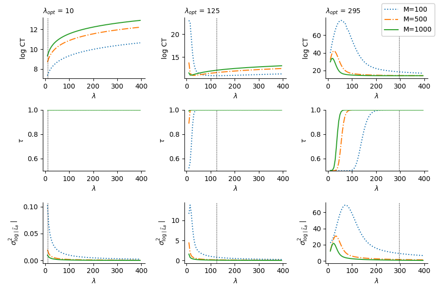
(a)

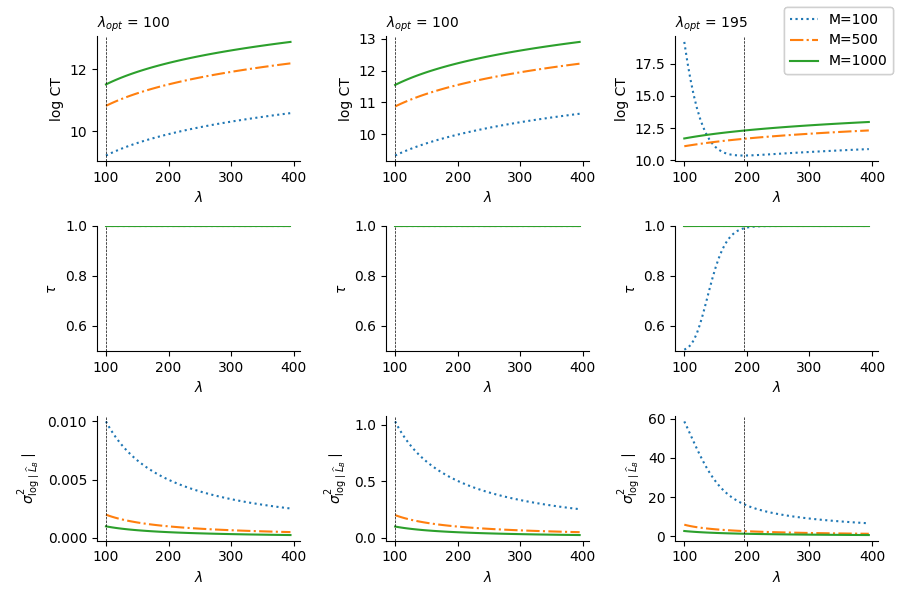
(b)

Figure 1: The effect of the number of blocks $\lambda$ on the logarithm of CT, $\tau$ and $\sigma^{2}_{\log\left|\widehat{L}_{B}\right|}$. The Poisson parameter $m$ is fixed at 1 for each set of panels (a,b). The correlation term is set to $\rho=0$ (upper panel), 0.99 (bottom panel). Columns from left to right, correspond to three different settings of $\gamma=10^{2}$, $100^{2}$, and $500^{2}$. The top, middle and last rows of each panel show log CT (14), the probability of obtaining a positive estimator $\tau(m,\lambda,M)$ (see Lemma 2) and the variance of log of the absolute value of the likelihood estimate. The vertical line on each plot represents $\lambda_{\mathrm{opt}}$, the optimal $\lambda$, which minimises the logarithm of CT among three settings.

Figure 1 shows the effects of the number of blocks ($\lambda$) and Monte Carlo samples ($M$) on the logarithm of CT, $\tau$ and $\sigma^{2}_{\log\left\lvert\widehat{L}_{B}\right\rvert}$. We consider the three cases $\gamma=10^{2},100^{2},500^{2}$ (left to right columns respectively) which show that the optimal $\lambda$ (corresponding to minimal CT) varies with different values of $M$ and increases with $\gamma$ (top row). The minimum CT is associated with a high probability of a positive estimator ($\tau$) (middle row). The last row indicates that $\sigma^{2}_{\log\left\lvert\widehat{L}_{B}\right\rvert}$ decreases as a function of $\lambda$. Comparing the top nine panels with the bottom nine, a high correlation $\rho=0.99$, reduces $\lambda_{\mathrm{opt}}$ from 295 (no correlation, $\rho=0$) to 195 for $\gamma=500^{2}$. Conversely, $\rho=0.99$ requires at least 100 blocks. So when the variance $\gamma$ is small, introducing a high correlation increases the CT as more blocks are required compared to the uncorrelated case. Our implementation follows the approach in Tran et al., (2016) which sets the correlation $\rho$ to a value close to 1. Comparing the first row of the top panel (a) in Figure 1 with that of the bottom (b), shows that a high correlation significantly reduces the CT per iteration for large $\gamma$.

The conclusion is that the optimal tuning depends on $\gamma$ in (3.3), which is the intrinsic variability of the population $\nu\widehat{Z}(\boldsymbol{\theta})$. For conservative tuning, in our applications we set $\gamma$ to a large value $\gamma_{\mathrm{max}}$ by using a grid search over possible $\boldsymbol{\theta}$. The tuning process starts with fixed values of $\lambda$ and $m$ to find the optimal value for $M$ that minimises (14). In Figure 2, we fix the values of $\lambda$ and $m$, with $\lambda=50,100$ (the corresponding $\rho$ are 0.98 and 0.99 respectively), and $m=1$. A standard optimiser is used to find the optimal value $M_{\mathrm{opt}}$ for each of the $\gamma$. The scattered dots in the left panel of Figure 2 plot various values of $\sqrt{\gamma}$ and the corresponding $M_{\mathrm{opt}}$. The figure shows that $M_{\mathrm{opt}}$ increases as a function of $\sqrt{\gamma}$ and similarly for the logarithm of CT as the right panel shows. To estimate the relationship between $M_{\mathrm{opt}}$ and $\sqrt{\gamma}$, a quadratic polynomial is fitted to the points in the left panel.

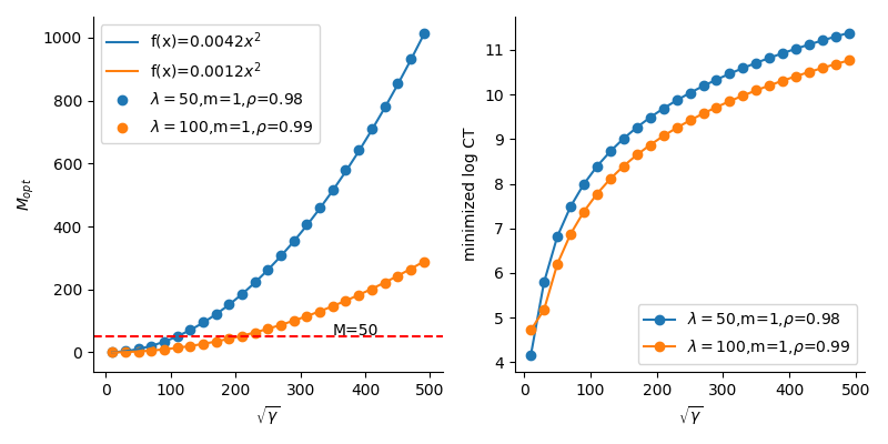
Figure 2: Left panel: The optimal value $M_{\mathrm{opt}}$ as a function of $\sqrt{\gamma}$. The lines are quadratic polynomials fitted to the scattered dots. The horizontal dashed line represents the threshold $M=50$, which is the minimal number of blocks required in the algorithm. Right panel: The minimised CT as a function of $\sqrt{\gamma}$.

The following tuning strategy is based on $\gamma_{\mathrm{max}}$, leading to a conservative choice of $M_{\mathrm{opt}}$.

1. Have a general idea of the posterior distribution of $\boldsymbol{\theta}$. This can be accomplished by conducting an exact method for a few iterations, optimising the posterior distribution by plugging the biased estimator ($1/\widehat{Z}(\boldsymbol{\theta})$), or applying an available approximate method.

2. Estimate the corresponding $\mathrm{Var}(\widehat{Z_{M}}(\boldsymbol{\theta}))/Z^{2}(\boldsymbol{\theta})$ using a grid search over possible $\boldsymbol{\theta}$ values based on results from Step 1. The estimator $\widehat{Z_{M}}(\boldsymbol{\theta})$ can be plugged into (3.3) to replace the unknown $Z(\boldsymbol{\theta})$. The variability induced by $\nu$ needs to be considered here. A conservative choice is $\gamma(\boldsymbol{\theta})=2M\mathrm{Var}(\widehat{Z_{M}}(\boldsymbol{\theta}))/\widehat{Z_{M}}^{2}(\boldsymbol{\theta})$. Section B in the supplement discusses this in more detail.

3. Obtain the maximum value $\gamma_{\mathrm{max}}(\boldsymbol{\theta})$ of $\gamma(\boldsymbol{\theta})$ from Step 2. A good starting point is to set $\lambda=100,m=1,\rho=0.99$ and $M_{\mathrm{opt}}=\max\{50,0.0012\times\gamma_{\max}(\boldsymbol{\theta})\}$.

   When $\gamma_{\max}(\boldsymbol{\theta})$ is small or moderately large, e.g. $\gamma_{\max}(\boldsymbol{\theta})<100^{2}$, having many blocks increases CT. A weaker correlation also produces an efficient algorithm with smaller CT. Another suitable setting is $\lambda=50,m=1,\rho=0.98$ and $M_{\mathrm{opt}}=\max\{50,0.0042\times\gamma_{\max}(\boldsymbol{\theta})\}$.

   For an even smaller $\gamma(\boldsymbol{\theta})$, the correlation can be relaxed further. In the Ising model example, setting $\lambda=10$ is sufficient when the variability is low; see Section 4.1 and Section C in the supplement.

3.4 An alternative pseudo-marginal approach under strong assumptions

If the estimator $\widehat{Z}(\boldsymbol{\theta})$ is normally distributed with a known variance, then an unbiased almost surely positive estimator may be derived using the penalty method in Ceperley and Dewing, (1999).

Suppose that $\widehat{Z}(\boldsymbol{\theta})\sim N(Z(\boldsymbol{\theta}),\sigma^{2}_{\widehat{Z}(\boldsymbol{\theta})})$, where $\sigma^{2}_{\widehat{Z}(\boldsymbol{\theta})}$ is the variance of $\widehat{Z}(\boldsymbol{\theta})$. Then $\exp(-\nu\widehat{Z}(\boldsymbol{\theta}))$ is log-normally distributed with expected value

$$E(\exp(-\nu\widehat{Z}(\boldsymbol{\theta})))=\exp\left(-\nu Z(\boldsymbol{\theta})+\frac{1}{2}\nu^{2}\sigma^{2}_{\widehat{Z}(\boldsymbol{\theta})}\right);$$

hence

$$\exp\left(-\nu\widehat{Z}(\boldsymbol{\theta})-\frac{1}{2}\nu^{2}\sigma^{2}_{\widehat{Z}(\boldsymbol{\theta})}\right)$$ (16)

is a positive unbiased estimator of $\exp(-\nu Z(\boldsymbol{\theta}))$. Thus, under the idealised assumptions that $\widehat{Z}(\boldsymbol{\theta})$ is normal with a known variance, we can use a pseudo-marginal algorithm to obtain samples from (3). However, in practice, $\widehat{Z}(\boldsymbol{\theta})$ is rarely normal and the variance must be estimated, so this method provides approximate samples in practice. It is outside the scope of this paper to study the resulting perturbation error.

The advantage of this method is that it is much faster than the BP estimator, because it only requires a single estimate of the normalising function. However, unlike our method, it is not simulation consistent. Section 4.1 implements this method as a fast alternative to our exact approach.

4 Simulation studies

We demonstrate the algorithm on three examples. The first is an Ising model, which is the usual benchmark example for doubly intractable problems as perfect sampling is available for this model on small grids. The example compares the signed PMMH with the BP estimator to other methods, including methods that sample from the exact posterior (3). The signed PMMH with the BP estimator generates simulation consistent results with less computing time for this example. The second example considers the Kent distribution, where the intractable normalising function is an infinite sum. To the best of our knowledge, exact Bayesian inference has not been considered for the Kent distribution due to its intractability. We show that, under certain settings, the Bayesian estimate obtained by our method outperforms those obtained by the maximum likelihood method and the method of moments with respect to the mean squared error. Finally, Section E in the supplement contains a third example considering a constrained Gaussian process, where the normalising function arises from constraining the process to be positive. We show that not accounting for the constraint, i.e. not taking into account the normalising function, leads to erroneous inference. The constrained Gaussian process and the Kent distribution are two examples of models where the non-pseudo methods (the auxiliary variable approaches that require perfect sampling) cannot be easily applied.

4.1 The Ising model

The Ising model (Lenz,, 1920; Ising,, 1925) has widespread applications, such as understanding phase transitions in thermodynamic systems (Fredrickson and Andersen,, 1984), interactive image segmentation in vision problems (Kolmogorov and Zabin,, 2004) and modelling small-world networks (Herrero,, 2002). It is the typical benchmark example in the literature to evaluate methods for tackling the doubly intractable problem; see e.g.  Møller et al., (2006); Lyne et al., (2015); Atchadé et al., (2013); Park and Haran, (2018). However, most of the existing methods use auxiliary variable approaches, as it is feasible to draw observations from the likelihood function perfectly, so-called perfect sampling. The pseudo-marginal methods such as RR and our approach do not require perfect sampling, which makes them applicable to more general problems. We implement and compare the results from the BP estimator, the bias-corrected estimator in Section 3.4 and the RR method for the Ising model.

Example 1 in Section 2.1: consider an $L\times L$ lattice with binary observations $y_{ij}$ of row $i$ and column $j$ ($y_{ij}\in\{-1,1\})$. The model is

$$\begin{aligned} p(\mathbf{y}|\theta)&=\frac{1}{Z(\theta)}\exp(\theta S(\mathbf{y})),\\ \text{with }S(\mathbf{y})&=\sum_{i=1}^{L}\sum_{j=1}^{L-1}y_{i,j}y_{i,j+1}+\sum_{i=1}^{L-1}\sum_{j=1}^{L}y_{i,j}y_{i+1,j}\\ \text{and }Z(\theta)&=\sum_{\mathbf{y}}\exp(\theta S(\mathbf{y}));\end{aligned}$$

$\theta$ is a scalar parameter and $S(\mathbf{y})$ imposes spatial dependence; a stronger interaction between observations is associated with a larger $\theta$. Obtaining $Z(\theta)$ is computationally expensive with a sum over $2^{L^{2}}$ possible configurations. The data simulations are conducted using perfect sampling (Propp and Wilson,, 1996), which samples exactly without evaluating the normalising function. Perfect sampling uses coupling to guarantee that the samples are generated from a Markov chain which has already converged to its equilibrium distribution. Following the settings in Park and Haran, (2018), two scenarios are considered on a $10\times 10$ grid, with $\theta=0.2$ and $0.43$; see Figure 3 for an illustration.

Figure 3: Illustrating an Ising model on a $10\times 10$ grid. The samples are drawn using perfect sampling with $\theta=0.2$ (left) and $\theta=0.43$ (right). The light and dark blue squares correspond to the values 1 and $-1$.

For all the algorithms considered, a uniform distribution on $[0,1]$ is selected as the prior for $\theta$. We adopt a random walk proposal centred at the current $\theta$ with a step size 0.07. The pseudo-marginal methods (RR, BP, and the bias-corrected estimator) require an unbiased estimator for $Z(\theta)$. We use annealed importance sampling (AIS) (Neal,, 2001) to obtain the estimate of $Z(\theta)$. The method starts by sampling from a tractable distribution (the prior) and ends at the intractable target (the posterior) via a sequence of intermediate distributions. The transitions between the distributions are completed via Gibbs updates and the weights associated with the transitions finally constitute the normalising function of interest; see Neal, (2001) for details of AIS in general and Section C in the supplement for its implementation for the Ising model.

To obtain the “gold” standard to evaluate the accuracy of the results, we follow Park and Haran, (2018), where an exchange algorithm with 1,010,000 iterations is performed. The first 10,000 iterations are discarded for burn-in and the remaining iterates are thinned so that 10,000 posterior samples remain.

$\theta_{\mathrm{true}}$ = 0.2
Method	Mean	95%HPD	IACT	Time(sec)	ESS/sec	$\lambda$	$\#$ particles
Gold	0.205	(0.075, 0.337)	1	-	-	-	-
BP	0.203	(0.066, 0.328)	7.43	676	4.0	10	100
Approx	0.204	(0.077, 0.331)	7.09	62	45.5	-	100
RR	0.202	(0.062, 0.328)	11.65	853	2.0	-	100
$\theta_{\mathrm{true}}$ = 0.43
Method	mean	95%HPD	IACT	time(sec)	ESS/sec	$\lambda$	$\#$ particles
Gold	0.433	(0.330, 0.533)	1.04	-	-	-	-
BP	0.435	(0.332, 0.545)	6.91	5877	0.5	50	100
Approx	0.441	(0.331, 0.549)	7.78	745	3.5	-	500
RR	0.432	(0.334, 0.549)	10.77	9134	0.2	-	500

Table 1: Inference results for the Ising model. All the chains, except for the “gold standard”, ran for 20,000 iterations using the algorithms described (Gold=exchange algorithm, BP= block-Poisson, Approx = bias-corrected estimator, RR = Russian roulette). For BP and RR, the mean estimates are corrected for the negative estimates using (12). The highest posterior density (HPD) intervals are calculated by the coda package in R. The IACT calculation is based on all the samples as the chains start at the true value. For BP and RR, the calculation of the IACT accounts for the negative estimates via (14). ESS/sec is the effective sample size per second. For BP, $\lambda$ refers to the number of blocks; $\#$ particles is the number of particles used in the AIS.

Table 1 summarises the simulation results. When $\theta=0.2$, all the estimates are close to that of the gold standard. The bias-corrected method has the smallest computing time and the best IACT. In the implementation, both the bias-corrected and BP methods exploit the block structure used in the signed block PMMH to control the variability in the log of the likelihood estimates between the current and the proposed value. As suggested in Section 3.3, the target correlation is set to no less than 0.98 with at least 50 blocks. We find that when $\theta=0.2$, the AIS method already gives a sufficiently low value for $\gamma_{\mathrm{max}}$. Hence, we reduced the number of blocks as per the tuning guidelines in Section 3.3 and set $\lambda=10$. When $\theta=0.43$, the strong dependence leads to a higher variability in $\widehat{Z}(\theta)$ (see Section C in the supplement). We increased the number of blocks to 50 for the BP estimator. To ensure a fair comparison, we also increased the number of particles in the importance samplers of AIS from 100 to 500 for the RR method to bring down the variance. The results of the BP and RR methods match well with that of the gold standard, whereas the bias-corrected method slightly overestimates the parameter. This may be due to the violation of the normality assumption of the bias-corrected estimator when $\theta$ is large. The bias-corrected method is 8 times faster than BP and 12 times faster than RR. Comparing the two exact methods with respect to ESS/sec, the BP estimator is around twice as efficient as the RR method.

To summarise, both the BP and the RR methods provide exact inference on the Ising model, with our method being about twice as efficient. We also propose the faster bias-corrected estimator in Section 3.4; however, this estimator is only unbiased if $\widehat{Z}(\theta)$ is normally distributed with known variance. The normality assumption is unlikely to hold for large $\theta$; see Figure 6 in the supplement, which shows that a large $\theta$ results in a heavily skewed distribution of $\widehat{Z}(\theta)$. This explains the bias incurred when $\theta_{\mathrm{true}}=0.43$.

4.2 The Kent distribution

Directional statistics involves the study of density functions defined on unit vectors in the plane or sphere. The Kent distribution, also known as the 5-parameter Fisher-Bingham distribution ($\mathrm{FB}_{5}$), is an analogue to the bivariate normal distribution to model asymmetrically distributed data on a spherical surface (Kent,, 1982). It has 5 parameters: $\boldsymbol{\gamma}_{1},\boldsymbol{\gamma}_{2},\boldsymbol{\gamma}_{3},\beta$, and $\kappa$, where $\boldsymbol{\gamma}_{1},\boldsymbol{\gamma}_{2},\boldsymbol{\gamma}_{3}$ form a 3-dimensional orthonormal basis, representing the mean, major and minor axes; $\kappa$ is the concentration parameter, and $\beta$ is a measure of its ovalness, with the constraint $0\leq\beta<\kappa/2$ to ensure that the distribution is unimodal.

Recall Example 2 in Section 2.1: the density of the Kent distribution is

$$f(\mathbf{y}|\boldsymbol{\gamma_{1}},\boldsymbol{\gamma_{2}},\boldsymbol{\gamma_{3}},\beta,\kappa)=\frac{1}{c(\kappa,\beta)}\exp\left\{\kappa\boldsymbol{\gamma_{1}}^{\top}\cdot\mathbf{y}+\beta\left[(\boldsymbol{\gamma_{2}}^{\top}\cdot\mathbf{y})^{2}-(\boldsymbol{\gamma_{3}}^{\top}\cdot\mathbf{y})^{2}\right]\right\},$$

where $\mathbf{y}\in\mathbb{R}^{3},\|\mathbf{y}\|=1$. The normalising function is

$$c(\kappa,\beta)=2\pi\sum_{j=0}^{\infty}\dfrac{\Gamma(j+0.5)}{\Gamma(j+1)}\beta^{2j}(0.5\kappa)^{-2j-0.5}I_{2j+0.5}(\kappa),$$

where $I_{\nu}(\cdot)$ is the modified Bessel function.

The normalising function is an intractable infinite sum. Due to the complex form of the density function, Kent, (1982) proposes a consistent moment estimator of the parameters. The moment estimation of $\boldsymbol{\gamma}_{i},i=1,2,3,$ is independent of $\beta$ and $\kappa$. Estimating $\beta$ and $\kappa$ requires an approximation that utilises the limiting case when $2\beta/\kappa$ is small or $\kappa$ is large, provided that the moment estimates of the $\boldsymbol{\gamma}_{i}$ are available. Alternatively, $\kappa$ and $\beta$ can be obtained numerically. Kume and Wood, (2005) adopt saddle point techniques to obtain the approximation for the normalising function. Kasarapu, (2015) uses the Bayesian framework to model a mixture of $\mathrm{FB}_{5}$ distributions. The infinite sum in $c(\kappa,\beta)$ is truncated in the sense that the successive term to be added is less than a prefixed threshold. However, this approach results in inexact Bayesian inference. In contrast, the signed block PMMH with the BP estimator provides exact Bayesian inference for the parameters.

We use the approach proposed by Papaspiliopoulos, (2011) to obtain an unbiased estimator for $c(\kappa,\beta)$. Rewrite $c(\kappa,\beta)$ as $\sum_{j=0}^{\infty}\phi_{j}(\kappa,\beta)$; then the estimator $\widehat{c}(\kappa,\beta)=\phi_{k}/q_{k}$ is unbiased, where $k$ is a non-negative discrete random variable with probability mass function $q_{k}$. Either a Poisson or a geometric distribution is suitable, as $k$ is a non-negative integer. It is straightforward to verify that $E(\widehat{c}(\kappa,\beta))=\sum_{k}\phi_{k}/q_{k}\times q_{k}=c(\kappa,\beta)$. As $\phi_{j}(\kappa,\beta)$ is a decreasing function in $j$, to reduce the variability, we compute the first $K$ terms exactly and perform a truncation of the remaining terms. Specifically, $c(\kappa,\beta)$ is decomposed as

$$\sum_{j=0}^{K-1}\phi_{j}(\kappa,\beta)+\sum_{j=K}^{\infty}\phi_{j}(\kappa,\beta).$$

The first sum is evaluated, and the second is estimated via the truncation procedure described above.

We apply the parameterisation in Kasarapu, (2015), where the orthonormal basis $\boldsymbol{\gamma}_{1},\boldsymbol{\gamma}_{2},\boldsymbol{\gamma}_{3}$ is reparameterised as $\psi\in[0,\pi],\alpha\in[0,2\pi],\eta\in[0,\pi]$. An adaptive Gaussian random walk proposal is used for all the parameters with the optimal covariance matrix proposed in Garthwaite et al., (2016). To accommodate such a proposal, we further transform $\psi,\alpha,\eta$ into $\psi^{*},\alpha^{*},\eta^{*}$ which take unconstrained values using the following transformations:

$$\psi^{*}=\log\left(\frac{\psi}{\pi-\psi}\right);\alpha^{*}=\log\left(\frac{\alpha}{2\pi-\alpha}\right)\quad{\rm and}\quad\eta^{*}=\log\left(\frac{\eta}{\pi-\eta}\right).$$

We also work with the logarithms of $\beta$ and $\kappa$ as they are unconstrained.

We follow Dowe et al., (1996) and set the prior for $\kappa$ as $4\kappa^{2}/\pi(1+\kappa^{2})^{2}$. For a given $\kappa$, the prior for $\beta$ is uniform on $[0,\kappa/2)$. The priors for $\psi$, $\alpha$ and $\eta$ follow Kasarapu, (2015). The joint prior on all the parameters, $\psi,\alpha,\eta,\beta$ and $\kappa$ is

$$\pi(\psi,\alpha,\eta,\beta,\kappa)=\dfrac{2\kappa\sin\alpha}{\pi^{3}(1+\kappa^{2})^{2}}\mathbbm{1}(0\leq 2\beta/\kappa<1).$$

In the simulation, we generate $n$ observations from $\mathrm{FB}_{5},$ with different settings for $\beta$ and $\kappa$. The data generation is performed by the R package Directional, which implements the acceptance-rejection method in Kent et al., (2013). We set $n=$ 10, 100, 1,000 in combination with $\beta/\kappa=$ 0.01, 0.25, 0.49, with $\kappa$ fixed as 5. The lower and the upper bounds for $\beta/\kappa$ are 0 and 0.5 to ensure unimodality of the data (Kent,, 1982).

		$n=10$			$n=100$			$n=1{,}000$
$\beta/\kappa$	Method	$\beta$	$\kappa$	$\beta/\kappa$	$\beta$	$\kappa$	$\beta/\kappa$	$\beta$	$\kappa$	$\beta/\kappa$
$0.01$	Bayesian	1.33	2.40	0.22	0.45	0.50	0.09	0.11	0.17	0.02
	Moment	1.48	4.01	0.16	0.25	0.55	0.05	0.05	0.16	0.01
	MLE	2.29	4.30	0.26	0.47	0.57	0.09	0.11	0.17	0.02
$0.25$	Bayesian	0.64	2.20	0.04	0.38	0.55	0.07	0.11	0.16	0.02
	Moment	1.01	3.69	0.09	0.63	0.54	0.13	0.65	0.17	0.13
	MLE	2.00	4.18	0.16	0.36	0.60	0.06	0.35	0.24	0.07
$0.49$	Bayesian	1.28	1.99	0.22	0.42	0.57	0.06	0.14	0.19	0.02
	Moment	1.38	3.27	0.27	1.48	0.59	0.28	1.50	0.46	0.28
	MLE	1.73	3.79	0.17	0.42	0.60	0.06	0.98	0.59	0.19

Table 2: Simulation results for 100 independent replications of a $\mathrm{FB}_{5}$ distribution. The numbers are the RMSEs with respect to the true values. Boldface numbers identify the lowest RMSE among the three methods (Bayesian, Moment, MLE).

Table 2 shows the RMSE with regard to the true values for the three methods based on 100 independent replicates. “Bayesian” refers to the signed block PMMH with the BP estimator algorithm. The selected hyperparameters are $\lambda=20$ (number of blocks), $m=1$ (Poisson mean value of BP), and $K=10$ (the number of truncated terms computed exactly in the estimation of the normalising function). A Poisson distribution with mean value 1 is used for the truncation. “Moment” refers to the moment estimates and “MLE” is based on our modification of the function kent.mle of the R package Directional, where the original version uses the moment estimates of $\gamma$’s. We use an optimiser on the transformed parameters to obtain the MLE of all the parameters in the modified version. For the Bayesian method, the RMSE is calculated using the posterior mean with the sign correction in (12). For a small number of observations ($n=10$), our method yields the smallest RMSE amongst all three methods.

Comparing the results of different $\beta/\kappa$ combinations, the moment estimator gives the best RMSE for $\beta/\kappa=0.01,$ and our method is superior to the other two when the ratio approaches 0.49, where the assumption underlying the moment estimator is almost violated. The MLE method uses the saddle point technique (Kume and Wood,, 2005) to approximate the likelihood. Unlike the moment estimation, the MLE method does not assume the limiting case where $2\beta/\kappa$ is small or $\kappa$ is large. Its performance gets closer to the Bayesian method for $\beta/\kappa=0.01$ with many observations. However, MLE has the worst performance on small data sets ($n=10$) due to a large standard error. As $\beta/\kappa$ increases, it outperforms the moment estimator, but is inferior to the Bayesian method.

The simulation study shows that the signed block PMMH with the BP estimator performs the best when the sample size is small. It also has the lowest RMSE when $\beta/\kappa$ approaches the limiting value 0.5. We conclude that the Bayesian approach using our method is a competitive alternative to the standard methods used for the Kent distribution in the literature.

5 An empirical study on spherical data

We now analyse four real spherical datasets using the Kent distribution and our method. Recall that the non-pseudo marginal approaches cannot be applied to this model. Each dataset contains samples from two groups, which are formed naturally from the sample collection process. Figure 4 plots the spherical datasets.

1. Palaeomagnetic (Palaeo) (Wood,, 1982): Thirty three estimates of previous magnetic pole positions were obtained using palaeomagnetic techniques. Each estimate is associated with a different site in Tasmania. The data is originally from Schmidt, (1976) and the author points out that the data is likely to fall mainly into two groups of distinct geographical regions. Following Figueiredo, (2009), the first group contains the observation indices 9, 10, 11, 12, 14, 16, 23, 24, 30.

2. Magnetic (Fisher et al.,, 1993, Table B8): Measurements of magnetic remanence from a set of 62 specimens is obtained. The specimens are from Mesozoic Dolerite from Prospect, New South Wales, after successive partial demagnetisation stages ($200^{\circ}$ and $350^{\circ}$). An experiment was conducted to determine the blocking temperature spectrum of the magnetisation components.

3. Sandstone (Fisher et al.,, 1993, Table B23): Measurements of natural remanent magnetisation in Old Red Sandstone rocks in Pembrokeshire, Wales. The measurements consist of specimens from two sites with the number of observations 35 and 13, respectively.

4. Stone (Fisher et al.,, 1993, Table B25): Measurements of the longest axis and shortest axis (101 observations) orientations of tabular stones on a slope at Windy Hills, Scotland.

Figure 4: Illustration of the datasets. Green points and red points refer to the observations from groups 1 and 2, respectively.

The two groups are modelled separately by assuming a non-hierarchical structure on the prior for all the parameters. The data is modelled in the same way as in Section 4.2 using the density function in (2).

Table 3 summarises the results. We first note that the three methods estimate the same quantity. The gap between the Bayesian and ML estimates is narrower for the bigger datasets (Magnetic, Stone). The moment estimates are far from the MLE and the Bayesian results, even for the bigger datasets. Since $\beta/\kappa$ is close to 0.5 for the Magnetic dataset, the moment estimate is unreliable. This result is supported by the simulation results in Section 4.2. The second result is that the confidence intervals for the moment estimates and the MLE, especially for small datasets (Palaeo, Sandstone), are wider than the Bayesian intervals. The Bayesian credible interval is constructed using the posterior distribution. For the MLE and moment estimates, we obtain the confidence intervals using the non-parametric bootstrap (Efron,, 1992). By construction, the intervals have different interpretations (frequentist vs Bayesian); however, both intervals are expected to be close when the number of observations is sufficiently large. Table 3 confirms this for the bigger dataset Stone, where the MLE and Bayesian intervals are close to each other. The moment estimates again seem to be less reliable for $\beta$. A larger $\kappa$ indicates the observations are more concentrated. For small datasets, the non-parametric bootstrap is likely to draw the same observation multiple times, resulting in a concentrated data pattern and a correspondingly large estimate of $\kappa$.

Palaeo	group 1 ($n=9$)			group 2 ($n=24$)
	$\beta$	$\kappa$	$\beta/\kappa$	$\beta$	$\kappa$	$\beta/\kappa$
Bayesian	2.78	18.25	0.16	3.86	33.89	0.11
	(0.20,11.64)	(7.92,38.55)	(0.01,0.41)	(0.27,12.76)	(21.33,50.48)	(0.01,0.32)
Moment	4.03	26.54	0.15	5.88	39.84	0.15
	(1.11,98.84)	(18.96,223.76)	(0.05,0.46)	(1.24,30.51)	(28.16,92.60)	(0.04,0.35)
MLE	4.55	26.65	0.17	6.44	40.02	0.16
	(0.78,106.84)	(18.96,223.02)	(0.04,0.50)	(1.06,34.34)	(28.25,96.38)	(0.03,0.38)
Magnetic	group 1 ($n=62$)			group 2 ($n=62$)
	$\beta$	$\kappa$	$\beta/\kappa$	$\beta$	$\kappa$	$\beta/\kappa$
Bayesian	7.32	15.23	0.49	15.77	32.04	0.49
	(5.28,10.03)	(11.18,20.34)	(0.43,0.50)	(11.17,21.58)	(22.95,43.29)	(0.46,0.50)
Moment	4.55	12.99	0.35	8.87	23.22	0.38
	(2.58,10.73)	(8.21,26.72)	(0.31,0.40)	(5.28,20.53)	(14.77,49.06)	(0.35,0.42)
MLE	8.24	16.49	0.50	15.57	31.13	0.50
	(4.76,16.95)	(9.57,34.04)	(0.49,0.50)	(9.82,33.12)	(19.65,66.23)	(0.49,0.50)
Sandstone	group 1 ($n=36$)			group 2 ($n=13$)
	$\beta$	$\kappa$	$\beta/\kappa$	$\beta$	$\kappa$	$\beta/\kappa$
Bayesian	1.48	20.31	0.07	8.54	47.08	0.19
	(0.08,5.68)	(14.51,28.33)	(0.00,0.23)	(0.70,27.20)	(24.69,89.95)	(0.02,0.39)
Moment	2.07	22.36	0.09	18.45	68.94	0.27
	(0.70,16.37)	(13.38,64.33)	(0.04,0.30)	(8.76,67.07)	(54.64,188.26)	(0.11,0.41)
MLE	2.42	22.44	0.11	20.15	70.18	0.29
	(0.00,17.93)	(13.41,65.55)	(0.00,0.36)	(7.90,76.18)	(55.30,199.75)	(0.09,0.44)
Stone	group 1 ($n=101$)			group 2 ($n=101$)
	$\beta$	$\kappa$	$\beta/\kappa$	$\beta$	$\kappa$	$\beta/\kappa$
Bayesian	0.52	4.19	0.13	1.06	2.18	0.49
	(0.05,1.32)	(3.37,5.12)	(0.01,0.30)	(0.79,1.34)	(1.64,2.72)	(0.44,0.50)
Moment	0.23	4.29	0.05	0.41	1.99	0.21
	(0.08,0.54)	(3.33,6.23)	(0.02,0.11)	(0.30,0.52)	(1.79,2.30)	(0.15,0.24)
MLE	0.60	4.32	0.14	1.10	2.19	0.50
	(0.15,1.91)	(3.38,6.31)	(0.03,0.50)	(0.92,1.30)	(1.85,2.61)	(0.50,0.50)

Table 3: Results for the Bayesian, moment and MLE approaches for all the datasets. The Bayesian estimate is the posterior mean. The numbers in brackets are the 95% confidence (credible for Bayesian) intervals. For the moment estimates and MLE, the confidence intervals are obtained using the bootstrap (Efron,, 1992) with 1,000 repetitions for each.

We use 5-fold cross validation to test the models’ performance. To avoid sampling bias, the splitting is done for both groups. Denote the training and test sets as $\mathbf{y}_{\mathrm{train},g}$ and $\mathbf{y}_{\mathrm{test},g},$ with $g$ the group membership $g\in\{1,2\}$. After fitting the models using $\mathbf{y}_{\mathrm{train},g}$, the prediction for an observation $\mathbf{y}_{i}$ averaged over the posterior distribution of $\boldsymbol{\theta}_{g}=\{\beta,\kappa,\psi,\alpha,\eta\}$ is

$$p(\mathbf{y}_{i}|\mathbf{y}_{\mathrm{train},g})=\int_{\boldsymbol{\theta}}p(\mathbf{y}_{i}|\boldsymbol{\theta}_{g})p(\boldsymbol{\theta}_{g}|\mathbf{y}_{\mathrm{train},g})d\boldsymbol{\theta}_{g}.$$

If $p(\mathbf{y}_{i}|\mathbf{y}_{\mathrm{train},1})>p(\mathbf{y}_{i}|\mathbf{y}_{\mathrm{train},2})$, $\mathbf{y}_{i}$ is classified as being in group 1, and conversely if the inequality is reversed. Section D in the online supplement provides more details.

			Train accuracy			Test accuracy
data	grp1	grp2	Bayesian	Moment	MLE	Bayesian	Moment	MLE
Palaeo	9	24	0.985	0.985	0.985	0.943	0.943	0.943
			(0.008)	(0.008)	(0.008)	(0.031)	(0.031)	(0.031)
Magnetic	62	62	0.554	0.561	0.548	0.507	0.502	0.501
			(0.011)	(0.014)	(0.015)	(0.006)	(0.034)	(0.037)
Sandstone	36	13	0.943	0.953	0.953	0.920	0.920	0.880
			(0.013)	(0.014)	(0.014)	(0.072)	(0.052)	(0.066)
Stone	101	101	0.892	0.877	0.890	0.886	0.861	0.896
			(0.002)	(0.003)	(0.001)	(0.005)	(0.011)	(0.005)

Table 4: Results of 5-fold cross validation on the four datasets. “grp1”,“grp2” are the number of observations for the corresponding group. Accuracy on the training and test data is the average value of the 5 folds, with the standard error in brackets. “Train accuracy” and “Test accuracy” state the proportion of correct predictions in all predictions made for the corresponding dataset. The boldface numbers represent the method(s) with the highest accuracy.

Table 4 shows the prediction accuracy on the training and test datasets. There is no notable difference in terms of the prediction accuracy between the methods across the datasets. One possible reason is that the parameters of one group are distinct from that of the other group, so that minor differences in parameter estimates do not affect the classification.

6 Conclusions

We propose the signed block PMMH with the block-Poisson estimator to carry out exact inference in general doubly intractable problems. Our method requires only an unbiased estimator of the normalising function, which makes it applicable to a wider range of problems than its competitors, which often require perfect sampling from the model.

Compared with the Russian roulette method in Lyne et al., (2015), the block-Poisson estimator achieves a smaller variance of the logarithmic difference in the likelihood estimates in the MH acceptance ratio by its use of correlated pseudo-marginal updates. Moreover, the Russian roulette method lacks guidelines on how to tune its hyperparameters. We derive heuristic guidelines based on analytical statistical properties of our estimator. The Ising model example in Section 4.1 suggests that our approach is about twice as efficient as the Russian roulette method.

Despite its wide applicability, the signed PMMH algorithm (with both block-Poisson and Russian roulette methods) is computationally costly when unbiasedly estimating the normalising function. The Ising model example shows that AIS is required multiple times during each iteration for both the block-Poisson and Russian roulette methods. This prevents the computing time of the PM methods being competitive with other methods which do not require estimating the normalising function. However, the algorithm gives exact inference with minimal assumptions on the structure of the model and therefore applies to a wider range of problems.

When the normalising function is an infinite sum as in the Kent distribution, the block-Poisson estimator can be obtained relatively cheaply, making the signed block PMMH with the block-Poisson estimator computationally efficient. Our proposed method enables the first exact Bayesian analysis on the Kent distribution. Moreover, for some settings of the Kent distribution, we show that the Bayesian estimator is superior to the maximum likelihood and method of moments estimators.

Appendix A Properties of the block-Poisson estimator

Proof.

The block-Poisson estimator is expressed as

$$\widehat{L}_{B}(\boldsymbol{\theta})=\prod_{l=1}^{\lambda}\exp(\xi_{l}(\boldsymbol{\theta}))$$

with

$$\exp(\xi_{l}(\boldsymbol{\theta}))=\exp(a/\lambda+m)\prod_{h=1}^{\chi_{l}}\dfrac{\widehat{B}^{(h,l)}(\boldsymbol{\theta})-a}{m\lambda},$$

where $\lambda$ is the number of blocks with $\chi_{l}\sim\mathrm{Pois}(m)$ and $a$ is an arbitrary constant. For notational convenience, dependence on $\boldsymbol{\theta}$ is omitted for $\widehat{L}_{B}$, $\widehat{B}$ and $\xi$.

The following proofs closely follow the proofs in Quiroz et al., (2021, Section S8) who assume $m=1$, whereas here $m$ can be any non-negative integer. The two properties below are useful for the proof. Suppose that $X\sim\mathrm{Pois}(m)$ and $A<\infty$. Then,

1. $E_{X}(A^{X})=\exp((A-1)m)$.

2. $\mathrm{Var}_{X}(A^{X})=\exp(-m)[\exp(A^{2}m)-\exp(2Am-m)]$.

Proof of unbiasedness

$$E(\exp(\xi_{l})) =\exp(a/\lambda+m)E\Bigg{[}\prod_{h=1}^{\chi_{l}}\dfrac{\widehat{B}^{(h,l)}-a}{m\lambda}\Bigg{]}$$

$$=\exp(a/\lambda+m)E_{\chi}E_{\widehat{B}|\chi}\Bigg{[}\prod_{h=1}^{\chi_{l}}\dfrac{\widehat{B}^{(h,l)}-a}{m\lambda}\Bigg{]}$$

$$=\exp(a/\lambda+m)E_{\chi}\Bigg{[}\dfrac{B-a}{m\lambda}\Bigg{]}^{\chi}$$

$$=\exp(a/\lambda+m)\exp((B-a)/\lambda-m)$$

$$=\exp(B/\lambda).$$

Hence, $E(\widehat{L}_{B})=\exp(B)$, as $\xi_{1},\dots,\xi_{\lambda}$ are independent.

In the implementation, we use $a=\widehat{B}-m\lambda$, where $\widehat{B}$ is an estimate of $B$ which is independent of $\widehat{B}^{(h,l)}$. Such a choice of $a$ preserves the unbiasedness of the block Poisson estimator.

Treating $a$ as a random variable, the expectation of the block-Poisson estimator can be expressed as

$$E(\widehat{L}_{B}(\boldsymbol{\theta}))=E_{a}E_{\xi_{1},\dots,\xi_{\lambda}|a}\prod_{l=1}^{\lambda}\exp(\xi_{l}(\boldsymbol{\theta}))=E_{a}\left(\prod_{l=1}^{\lambda}E_{\xi_{l}|a}\exp(\xi_{l}(\boldsymbol{\theta}))\right).$$

The conditional expectation of $E_{\xi_{l}|a}\exp(\xi_{l})$ is (omitting the dependence on $\boldsymbol{\theta}$)

$$E_{\xi_{l}|a}\exp(\xi_{l})=E_{\xi_{1}|a}\exp(a/\lambda+m)\prod_{h=1}^{\chi_{l}}\dfrac{\widehat{B}^{(h,l)}-a}{m\lambda}.$$

The conditional expectation is the same as the derived $E(\exp(\xi_{l}))$, which is independent of $a$ as $a$ cancels out in the process. Hence, treating $a$ as a random variable still guarantees the unbiasedness of the block-Poisson estimator.

Derivation of the variance

From the definition of $\widehat{L}_{B}$,

$$\mathrm{Var}(\widehat{L}_{B}) =\mathrm{Var}\left(\prod_{l=1}^{\lambda}\exp(\xi_{l})\right).$$

For a collection of independent random variables $\exp(\xi_{1}),\ldots,\exp(\xi_{\lambda})$,

$$\mathrm{Var}\left(\prod_{l=1}^{\lambda}\exp(\xi_{l})\right)=\prod_{l=1}^{\lambda}\left(\mathrm{Var}(\exp(\xi_{l}))+E(\exp(\xi_{l}))^{2}\right)-\prod_{l=1}^{\lambda}E(\exp(\xi_{l}))^{2}$$

with

$$\mathrm{Var}(\exp(\xi_{l})) =\exp(a/\lambda+m)\left[E_{\chi}\mathrm{Var}_{\widehat{B}|\chi}\left(\prod_{h=1}^{\chi}\dfrac{\widehat{B}^{(h,l)}-a}{m\lambda}\right)+\mathrm{Var}_{\chi}E_{\widehat{B}|\chi}\left(\prod_{h=1}^{\chi}\dfrac{\widehat{B}^{(h,l)}-a}{m\lambda}\right)\right].$$

For the first term in the brackets, making the use of independence of $\widehat{B}^{(h,l)},h=1,\dots,\chi_{l}$,

$$\mathrm{Var}_{\widehat{B}|\chi}\left(\prod_{h=1}^{\chi}\dfrac{\widehat{B}^{(h,l)}-a}{m\lambda}\right)$$

is simplified as

$$\mathrm{Var}_{\widehat{B}|\chi}\left(\prod_{h=1}^{\chi}\dfrac{\widehat{B}^{(h,l)}-a}{m\lambda}\right) =\prod_{h=1}^{\chi}\left[\mathrm{Var}\left(\dfrac{\widehat{B}^{(h,l)}-a}{m\lambda}\right)+E\left(\dfrac{\widehat{B}^{(h,l)}-a}{m\lambda}\right)^{2}\right]$$

$$-\prod_{h=1}^{\chi}E\left(\dfrac{\widehat{B}^{(h,l)}-a}{m\lambda}\right)^{2}$$

$$=\prod_{h=1}^{\chi}\left(\frac{\sigma_{B}^{2}+(B-a)^{2}}{(m\lambda)^{2}}\right)-\left(\frac{B-a}{m\lambda}\right)^{2\chi}.$$

Taking the expectation with regard to $\chi$ and using property (i) twice for the two terms, we have

$$E_{\chi}\mathrm{Var}_{\widehat{B}|\chi}\left(\prod_{h=1}^{\chi}\dfrac{\widehat{B}^{(h,l)}-a}{m\lambda}\right) =\exp\left[\left(\frac{\sigma_{B}^{2}+(B-a)^{2}}{(m\lambda)^{2}}-1\right)m\right]-\exp\left[\left(\frac{(B-a)^{2}}{(m\lambda)^{2}}-1\right)m\right]$$

$$=\exp\left[\left(\frac{(B-a)^{2}}{(m\lambda)^{2}}-1\right)m\right]\left[\exp\left(\frac{\sigma_{B}^{2}}{m\lambda^{2}}\right)-1\right].$$

The second term is derived similarly,

$$\mathrm{Var}_{\chi}E_{\widehat{B}|\chi}\left(\prod_{h=1}^{\chi}\dfrac{\widehat{B}^{(h,l)}-a}{m\lambda}\right) =\mathrm{Var}_{\chi}\left(\frac{B-a}{m\lambda}\right)^{\chi}$$

$$=\exp\left(-m+\frac{(B-a)^{2}}{m\lambda^{2}}\right)-\exp\left(2(B-a)/\lambda-2m\right).$$

Combining the two terms, we have

$$\mathrm{Var}(\exp(\xi_{l}))=\exp\bigg{[}\frac{(B-a)^{2}+\sigma_{B}^{2}}{m\lambda^{2}}-m\bigg{]}-\exp(2(B-a)/\lambda-2m).$$

Deriving $E(\exp(\xi))^{2}$ is straight forward,

$$E(\exp(\xi_{l}))^{2} =\left[E_{\chi}E_{B|\chi}\prod_{h=1}^{\chi}\left(\frac{\widehat{B}^{(h,l)}-a}{m\lambda}\right)\right]^{2}$$

$$=\exp(2(B-a)/\lambda-2m).$$

Combining all the terms, after some algebra, the variance of the block-Poisson estimator is

$$\mathrm{Var}(\widehat{L}_{B})=\exp\left[\frac{(B-a)^{2}+\sigma_{B}^{2}}{m\lambda}+2a+m\lambda\right]-\exp(2B).$$

Choice of the constant $a$

The optimal value minimising $\mathrm{Var}(\widehat{L}_{B})$ is $a=B-m\lambda$, which is obtained by solving the equation $\partial\widehat{L}_{B}/\partial a=0$. ∎

The proof of Lemma 2 is the same as Lemma 3 in Quiroz et al., (2021).

Proof of Lemma 3.

The variance of the log of the likelihood estimator is

$$\mathrm{Var}(\log\lvert\widehat{L}_{B}\rvert) =\mathrm{Var}\bigg{(}\sum_{l=1}^{\lambda}\sum_{h=1}^{\chi_{l}}\log\left\lvert\frac{\widehat{B}^{(h,l)}-a}{m\lambda}\right\rvert\bigg{)}$$

$$=E_{\chi_{1,\ldots,\lambda}}V_{B|\chi_{1,\ldots\lambda}}\log\left\lvert\frac{\widehat{B}^{(h,l)}-a}{m\lambda}\right\rvert+\mathrm{Var}_{\chi_{1,\ldots,\lambda}}E_{B|\chi_{1,\ldots\lambda}}\log\left\lvert\frac{\widehat{B}^{(h,l)}-a}{m\lambda}\right\rvert.$$

Suppose $\widehat{B}^{(h,l)}\sim N(B,\sigma_{B}^{2})$ and $a=B-m\lambda$; then

$$\log\left\lvert\frac{\widehat{B}^{(h,l)}-a}{m\lambda}\right\rvert =\log\left\lvert\frac{\sigma_{B}Z}{m\lambda}+1\right\rvert$$

$$=\log(\sigma_{B}/(m\lambda))+\log\lvert Z+m\lambda/\sigma_{B}\rvert$$

$$=\log(\sigma_{B}/(m\lambda))+\frac{1}{2}\log((Z+m\lambda/\sigma_{B})^{2})$$

$$=\log(\sigma_{B}/(m\lambda))+\frac{1}{2}\log W^{(h,l)},\quad W^{(h,l)}\sim\chi^{2}(1,(m\lambda/\sigma_{B})^{2}),$$

where $\chi^{2}(k,\lambda)$ denotes the non-central $\chi^{2}$ distribution with $k$ degrees of freedom and non-centrality parameter $\lambda$. Lemma S12 in Quiroz et al., (2021) provides the moments of $\log W$.

Let $\eta_{B}$ and $\nu_{B}^{2}$ be the expectation and the variance of $\log\left\lvert(\widehat{B}^{(h,l)}-a)/{m\lambda}\right\rvert$ respectively. We have

$$\eta_{B}=E\bigg{(}\log\left\lvert\frac{\widehat{B}^{(h,l)}-a}{m\lambda}\right\rvert\bigg{)} =\log(\sigma_{B}/(m\lambda))+\frac{1}{2}\log(2+E_{J}[\psi^{(0)}(0.5+J)],$$

$$\nu_{B}^{2}=\mathrm{Var}\bigg{(}\log\left\lvert\frac{\widehat{B}^{(h,l)}-a}{m\lambda}\right\rvert\bigg{)} =\frac{1}{4}\left[E_{J}[\psi^{(1)}(0.5+J)]+\mathrm{Var}_{J}[\psi^{(0)}(0.5+J)]\right],$$

where $J\sim\mathrm{Pois}((m\lambda)^{2}/2\sigma_{B}^{2})$ and $\psi^{(q)}$ is the polygamma function of order $q$.

Then,

$$\mathrm{Var}(\log\lvert\widehat{L}_{B}\rvert) =E_{\chi_{1,\ldots,\lambda}}\bigg{(}\sum_{l=1}^{\lambda}\chi_{l}\bigg{)}\nu^{2}_{B}+\mathrm{Var}_{\chi_{1,\ldots,\lambda}}\bigg{(}\sum_{l=1}^{\lambda}\chi_{l}\bigg{)}\eta_{B}$$

$$=m\lambda(\nu_{B}^{2}+\eta_{B}^{2}).$$

Furthermore, $\mathrm{Var}(\log\lvert\widehat{L}_{B}\rvert)<\infty$. Lemma 7 in Quiroz et al., (2021) derives the result. ∎

Appendix B Implementation details of the signed block PMMH with the BP estimator

This section gives the implementation details of Algorithm 1; it covers the construction of the BP estimator and the choice of the soft lower bound. In Section 3.3, the variance of $\gamma(\boldsymbol{\theta})=M\mathrm{Var}(-\nu\widehat{Z_{M}}(\boldsymbol{\theta}))$ is treated as a known value for hyperparameter tuning. The decomposition of $\gamma(\boldsymbol{\theta})$ is discussed below, which helps to understand the effect of the randomness in $\nu$.

Construction of the BP estimator

To implement the BP estimator, we first fix the hyperparameters $\lambda,m$ and $a$. For each of the blocks $h$, $h=1,\dots,\lambda$, we sample $\chi_{h}\sim\text{Pois}(m)$. Depending on the value of $\chi_{h}$, we need to have the same number of $-\nu\widehat{Z}$ estimates. The computation can be done in parallel. We can draw $\chi_{h}$ for all the possible $h$ values at one time, and the total replications of $-\nu\widehat{Z}$ required are $\sum_{h=1}^{\lambda}\chi_{h}$. Parallel computation can also be implemented within the individual estimation process for $\widehat{Z}$ locally, where the calculation of $M$ particles is executed simultaneously.

Choosing the lower bound in the BP estimator

The lower bound $a_{\mathrm{opt}}=-\nu Z-m\lambda$ for the BP estimator minimises the variance of the likelihood estimator. In the implementation, $Z$ is replaced by its estimate $\widehat{Z}$. Its computation is exactly the same as that of the $\widehat{Z}$s’ used in the estimator. We emphasise that it is necessary to estimate $\widehat{Z}$ independently to ensure that the estimator is unbiased.

Decomposition of $\gamma$

By (3.3),

$$\gamma(\boldsymbol{\theta})=M\nu^{2}\mathrm{Var}(\widehat{Z_{M}}(\boldsymbol{\theta}))=M\frac{\log(u)^{2}}{Z^{2}}\frac{\sigma_{Z}^{2}}{M}=\log(u)^{2}\dfrac{\sigma_{Z}^{2}}{Z^{2}}.$$

The dependence of $Z$, $\sigma_{Z}^{2}$ and $\gamma$ on $\boldsymbol{\theta}$ is omitted for simplicity. The equation above shows that $\gamma$ is determined by a constant $\log(u)^{2}$ and the coefficient of variation (CV) $\sigma_{Z}/Z$. The unconditional variance can also be derived by using the law of total variance, giving a similar conclusion as discussed below.

Effect of $\log(u)^{2}$: It is concerning that $\log(u)^{2}$ is unbounded as $u$ approaches 0. As Figure 5 shows, there is less than a 5% chance of $\log(u)^{2}>9$. Instead, as the equation above shows, the introduction of $u$ reduces the variance by a factor of around 2 with 50% probability as $\Pr(\log(u)^{2}<0.48)=0.5$. Furthermore, $\Pr(\log(u)^{2}<1)=0.63$, indicating that the variance does not increase with a probability greater than 0.6. The expectation of $\log(u)^{2}$ is around 2, i.e., on average, the effect of $u$ doubles the variance.

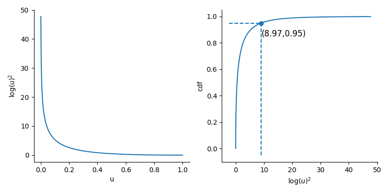
Figure 5: Left panel: plot of $\log(u)^{2}$ on $u\in(0,1]$. Right panel: the cdf of $\log(u)^{2}$ with $u\sim\text{Uniform}(0,1]$.

Effect of the coefficient of variation (CV) $\sigma_{Z}/Z$: The CV is difficult to estimate as both $\sigma_{Z}$ and $Z$ are unknown. The term $\sigma_{Z}^{2}/(MZ^{2})=\mathrm{CV}^{2}/M$ is often estimated by Monte Carlo integration as $\mathrm{CV}$ is an unknown quantity.

Conclusion: It is hard to obtain an analytical expression of $\gamma=\log(u)^{2}\mathrm{CV}^{2}$, where $\mathrm{CV}$ is estimated by Monte Carlo integration. There is uncertainty associated with $\log(u)^{2}$. Setting it to 2 is a conservative choice as $E(\log(u)^{2})\approx 2$.

Appendix C Details of the Ising model

C.1 An unbiased estimator for the normalising function

This section supplements the material on AIS sampling in Section 4.1. The likelihood function is $p(\mathbf{y}|\theta)=f(\mathbf{y}|\theta)/Z(\theta)$, with $f(\mathbf{y}|\theta)=\exp(\theta S(\mathbf{y}))$.

Consider the following intermediate kernel of the likelihood function

$$f_{i}(\mathbf{y}|\theta)=f(\mathbf{y}|\theta)^{\beta_{i}}p(\mathbf{y})^{1-\beta_{i}},i=0,\dots,N,$$

where $0=\beta_{0}<\beta_{1}<\dots<\beta_{N-1}<\beta_{N}=1$ and $p(\mathbf{y})=0.5^{L\times L}$. In the case of $\beta_{0}$, sampling from the prior density $f_{N}(\mathbf{y}|\theta)$ of $\beta_{0}$ is straightforward. By gradually increasing $\beta_{i}$, the generated data samples are drawn from the desired likelihood function $f_{N}(\mathbf{y}|\theta)=f(\mathbf{y}|\theta)$ after $N$ steps without knowing the normalising function. The algorithm starts by sampling $M$ particles from $f_{0}(\mathbf{y}|\theta)$, and proceeds with a certain transition probability to a new configuration for $\beta_{i}$ ($i=1,\dots,N-1)$ and terminates when $\beta_{N}=1$ is reached.

The transition to a new configuration $\mathbf{y}_{i+1,m}$ ($m=1,\dots,M$) from the current configuration $\mathbf{y}_{i,m}$ is completed by the following Gibbs update.

1. Select one random location $i,j$ out of a $L\times L$ grid.

2. Change the corresponding value of $y_{i,j}$ with probability

   $$p(y_{i,j}=1)=\dfrac{1}{1+\exp(-\beta_{i+1}\theta\sum y_{\rm neighbour})},$$

   where $y_{neighbour}$ refers to the points to the left, right, up and down of $y_{i,j}$.

3. Set the new configuration as $y_{i+1,m}$.

The final weight associated with particle $m$ (omitting $\theta$) is

$$w^{(m)}=\dfrac{f_{1}(\mathbf{y}_{0,m})}{f_{0}(\mathbf{y}_{1,m})}\dfrac{f_{2}(\mathbf{y}_{1,m})}{f_{1}(\mathbf{y}_{1,m})}\dots\dfrac{f_{n}(\mathbf{y}_{n-1,m})}{f_{n-1}(\mathbf{y}_{n-1,m})}.$$

The average of the importance weights $\sum_{m=1}^{M}w^{(m)}/N$ converges to the ratio of $Z_{1}(\theta)/Z_{0}(\theta)$, where $Z_{i}(\theta)$ corresponds the normalising function of $f_{i}(y|\theta)$.

We work with $\log w^{(m)}$ to avoid overflow problems. Parallel computation is possible because the particles are independent. Our description follows the supplementary code in Park and Haran, (2018) which uses OpenMP to implement the parallel computation. The re-evaluation of $S(\mathbf{y})$ from scratch can be computationally costly as it involves $O(L^{2})$ operations for each combination of $\beta_{i}$ and particle $m$. We modify the evaluation process by adding or subtracting the local updates of the selected location only. Such changes reduce the complexity to $O(1)$ and consequently decrease the computational time substantially.

C.2 The bias-corrected estimator

By introducing the auxiliary variable $\nu$, we transform the problem of unbiasedly estimating the reciprocal $Z(\theta)$ into the problem of unbiasedly estimating $\exp(-\nu Z(\theta))$. Ceperley and Dewing, (1999) discuss a method for debiasing $\exp(\cdot)$; Quiroz et al., later extend their estimator to subsampling. They call their estimator the approximately bias-corrected likelihood estimator. The core idea of the method is based on the normality assumption of $\widehat{Z}(\theta)$. It is well known that if $X\sim$ $\mathrm{log{-}normal}(\mu,\sigma^{2})$, then $E(X)=\exp(\mu+0.5\sigma^{2})$. Using this property of the log-normal distribution, the bias-corrected estimator is

$$\exp\left(-\nu\widehat{Z_{M}}(\theta)-\dfrac{\mathrm{Var}(-\nu\widehat{Z_{i}}(\theta))}{2M}\right),$$

where $\widehat{Z_{M}}(\theta)=\frac{1}{M}\sum_{i=1}^{M}\widehat{Z_{i}}(\theta)$.

C.3 The variability of the normalising function

The estimate $\widehat{Z}$ and its variance are crucial in hyperparameter tuning for the proposed algorithm. As the Ising model involves one parameter, it is feasible to study the variability of $\widehat{Z}$ by simulation. Figure 6 shows the estimates of the scaled $\widehat{Z}$ under different $\theta$ values, where $\widehat{Z}$ is rescaled by dividing by the sample mean of the replications. Each histogram is generated by 1,000 independent replications, each of which uses 100 particles in AIS with 4,000 intermediate transitions equally spaced between 0 and 1. The horizontal axis refers to the scaled $\widehat{Z}(\theta)$. As $\theta$ increases, the distribution of the scaled $\widehat{Z}$ is heavily skewed and the normality assumption appears to be invalid for $\theta>0.4$. Such violation explains the overestimation by the bias-corrected estimator for $\theta=0.43$ in the example in Section 4.1. Examining the range of the horizontal axis, the magnitude also increases sharply with $\theta$, which implies that a larger $\theta$ is associated with more variability in $\widehat{Z}$. Hence, more particles are required to estimate $\widehat{Z}$ as $\theta$ increases.

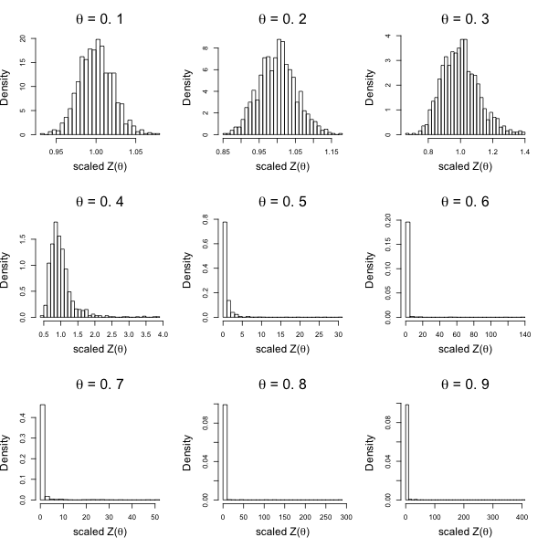
Figure 6: Histograms of scaled $Z(\theta)$ estimates on a $10\times 10$ 2D Ising model.

Appendix D Details of the Kent distribution

In Example 2 of Section 2.1, the density function of the Kent distribution is

$$p(\mathbf{y}|\boldsymbol{\theta})=\frac{1}{c(\beta,\kappa)}\exp\left\{\kappa\boldsymbol{\gamma}_{1}^{\top}\cdot\mathbf{y}+\beta\left[(\boldsymbol{\gamma}_{2}^{\top}\cdot\mathbf{y})^{2}-(\boldsymbol{\gamma}_{3}^{\top}\cdot\mathbf{y})^{2}\right]\right\}=\frac{f(\mathbf{y}|\boldsymbol{\theta})}{c(\beta,\kappa)},$$

with $\mathbf{y}=\{y_{1},y_{2},y_{3}\}$, $\sum_{i=1}^{3}y_{i}^{2}=1$ and $\boldsymbol{\theta}=\{\boldsymbol{\gamma}_{1},\boldsymbol{\gamma}_{2},\boldsymbol{\gamma}_{3},\beta,\kappa\}$; $\kappa>0,0\leq\beta<\kappa/2$. The parameters $\{\boldsymbol{\gamma}_{1},\boldsymbol{\gamma}_{2},\boldsymbol{\gamma}_{3}\}$ form a 3-dim orthonormal matrix with $\boldsymbol{\gamma}_{i},i=1,2,3$ is a $3\times 1$ vector.

For a 3-dimensional $\mathrm{FB}_{5}$ distribution, the normalising function is

$$c(\beta,\kappa)=2\pi\sum_{j=0}^{\infty}\dfrac{\Gamma(j+0.5)}{\Gamma(j+1)}\beta^{2j}(0.5\kappa)^{-2j-0.5}I_{2j+0.5}(\kappa)$$

.

Assume $n$ independent observations $\mathbf{y}_{1:n}:=\{y_{1},\ldots,y_{n}\}$ from a $\mathrm{FB}_{5}$ distribution, together with the auxiliary variables $\nu_{i}\sim\text{Expon}(c(\beta,\kappa)),i=1,\cdots,n$. The posterior distribution is

$$\pi(\boldsymbol{\theta},\nu_{1:n}|\mathbf{y}_{1:n}) \propto\pi(\boldsymbol{\theta})\prod_{i=1}^{n}f(\mathbf{y}_{i}|\boldsymbol{\theta})\exp\left(-\nu_{i}c(\beta,\kappa)\right)$$

$$=\pi(\boldsymbol{\theta})\exp\left(-\sum_{i=1}^{n}\nu_{i}c(\beta,\kappa)\right)\prod_{i=1}^{n}f(\mathbf{y}_{i}|\boldsymbol{\theta}).$$

The time to calculate the normalising function $c(\beta,\kappa)$ does not increase with the number of observations, and again we use the BP method to unbiasedly estimate $\exp(\cdot)$.

Classification prediction: In the empirical study, we assume that the $n$ independent observations are from a mixture of two groups of the Kent distribution with unknown parameters $\boldsymbol{\theta}_{g}=\{\boldsymbol{\gamma}_{1,g},\boldsymbol{\gamma}_{2,g},\boldsymbol{\gamma}_{3,g},\beta_{g},\kappa_{g}\},g=1,2$. Given the underlying group membership is provided and there is no hierarchical structure for the prior on $\boldsymbol{\theta}_{g}$, the posterior distribution for the parameters and the auxiliary variables is

$$\pi(\boldsymbol{\theta}_{1},\boldsymbol{\theta}_{2},\nu_{1:n,1:2}|\mathbf{y}_{1:n_{1},1},\mathbf{y}_{1:n_{2},2})\propto\prod_{g=1}^{2}\left[\pi(\boldsymbol{\theta}_{g})\exp\left(-\sum_{i=1}^{n_{g}}\nu_{i,g}c(\beta_{g},\kappa_{g})\right)\prod_{i=1}^{n_{g}}f(\mathbf{y}_{i,g}|\boldsymbol{\theta}_{g})\right];$$

$n_{g}$ is the number of observations belonging to group $g$ and the auxiliary variable $\nu_{i,g}\sim\text{Expon}(c(\beta_{g},\kappa_{g}))$.

For prediction, assign $\mathbf{y}_{i}$ to group 1 if $p(\mathbf{y}_{i}|\mathbf{y}_{train,1})>p(\mathbf{y}_{i}|\mathbf{y}_{train,2})$ and to group 2 otherwise. The density $p(\mathbf{y}_{i}|\mathbf{y}_{train,g})$ is evaluated as

$$p(\mathbf{y}_{i}|\mathbf{y}_{train,g}) =\int_{\boldsymbol{\theta}_{g}}p(\mathbf{y}_{i}|\boldsymbol{\theta}_{g})p(\boldsymbol{\theta}_{g}|\mathbf{y}_{train,g})d\boldsymbol{\theta}_{g}$$

$$=\int_{\boldsymbol{\theta}_{g}}\int_{\nu_{i}}p(\mathbf{y}_{i},\nu_{i}|\boldsymbol{\theta}_{g})p(\boldsymbol{\theta}_{g}|\mathbf{y}_{train,g})d\nu_{i}d\boldsymbol{\theta}_{g}$$

$$=\int_{\boldsymbol{\theta}_{g}}\int_{\nu_{i}}f(\mathbf{y}_{i}|\boldsymbol{\theta}_{g})\exp(-\nu_{i}c(\beta_{g},\kappa_{g}))p(\boldsymbol{\theta}_{g}|\mathbf{y}_{train,g})d\nu_{i}d\boldsymbol{\theta}_{g}$$

$$=\int_{\boldsymbol{\theta}_{g}}\int_{\nu_{i}}f(\mathbf{y}_{i}|\boldsymbol{\theta}_{g})E(\widehat{\exp}(-\nu_{i}c(\beta_{g},\kappa_{g})))p(\boldsymbol{\theta}_{g}|\mathbf{y}_{train,g})d\nu_{i}d\boldsymbol{\theta}_{g}.$$

The last equation is estimated by importance sampling using the proposal $\nu_{i}\sim\text{Expon}(\widehat{c}(\beta_{g},\kappa_{g}))$. The inner integral is estimated by

$$f(\mathbf{y}_{i}|\boldsymbol{\theta}_{g})\frac{1}{\widehat{c}(\beta_{g},\kappa_{g})}\frac{1}{M}\sum_{i=1}^{M}\frac{\widehat{\exp}(-\nu_{i}c(\beta_{g},\kappa_{g}))}{\exp(-\nu_{i}\widehat{c}(\beta_{g},\kappa_{g}))}.$$

The outer integral is computed by taking the average of the $\boldsymbol{\theta}_{g}$ iterates.

Appendix E A constrained Gaussian process

This section applies our method to a constrained Gaussian process.

A Gaussian process $\mathcal{GP}$ is a collection of random variables, such that every finite subcollection has a multivariate normal distribution. It defines a distribution over functions and is widely used as a prior in nonparametric regression (Williams and Rasmussen,, 2006). In this section, we consider a constrained $\mathcal{GP}$ process, where the constraint arise from the $\mathcal{GP}$ prior and not from the observations. Direct transformation of the data does not remove the constraints. Hence, conducting the constrained version of a $\mathcal{GP}$ regression is a challenging task compared with a normal $\mathcal{GP}$ regression. Specifically, we assume that $y=g(\mathbf{x})+\epsilon$, where $\mathbf{x}\in\mathbb{R}^{d}$, $g(\mathbf{x})\geq 0$ and $\epsilon\sim N(0,\sigma^{2})$. A constrained $\mathcal{GP}$ prior on $g(\mathbf{x})$ is proposed with the covariance of $g$ chosen as the squared exponential (SE) kernel combined with a diagonal matrix with small positive entries; $g(\mathbf{x})\sim\mathcal{GP}(0,K(\mathbf{x},\mathbf{x}^{\prime}|\alpha,\rho))\mathbbm{1}(g\geq 0)$ with

$$K(\mathbf{x},\mathbf{x}^{\prime}|\alpha,\rho)=\alpha^{2}\exp\left(-\frac{\left\|\mathbf{x}-\mathbf{x}^{\prime}\right\|^{2}}{2\rho^{2}}\right)+\tau^{2}\mathbbm{1}(\mathbf{x}=\mathbf{x}^{\prime}).$$ (17)

The constrained $\mathcal{GP}$ prior assumes that the function values follow

$$\mathbf{g}|\mathbf{x}_{1},\mathbf{x}_{2},\dots,\mathbf{x}_{n}\sim N(\mathbf{0},K(\mathbf{x},\mathbf{x}^{\prime}|\alpha,\rho))\mathbbm{1}(\mathbf{g}\geq\mathbf{0}),$$

where $\mathbf{x}=(\mathbf{x}_{1},\mathbf{x}_{2},\dots,\mathbf{x}_{n})^{\prime}$. The nugget effect $\tau^{2}$ is needed to prevent the determinant of a kernel matrix based on the SE kernel from being close to zero in high dimensions (Williams and Rasmussen,, 2006, pp. 97-98). Setting $\tau^{2}$ to a small positive number avoids this problem, and we set $\tau^{2}=0.05^{2}$. Section E.2 shows that the doubly intractable problem arises from the normalising function in the prior not the likelihood, which is different from the Ising model in Section 4.1.

To the best of our knowledge, this type of constraint has not been investigated in the literature; see the survey paper for the constrained $\mathcal{GP}$ in Swiler et al., (2020). Our example considers two cases. The first uses the $\mathcal{GP}$ process on a small dataset $(n=100)$. The second case considers a scalable $\mathcal{GP}$ on a larger dataset $(n=1{,}000)$, where it is computationally expensive to conduct exact inference.

E.1 Prior on the hyperparameters

The $\mathcal{GP}$ regression involves two stages. The first stage carries out inference about the hyperparameters $(\alpha,\rho,\sigma^{2})$ and the second stage predicts the process $g$ for a new location $\mathbf{x}^{*}$. We use a Bayesian approach and make the predictions based on the iterates to compute $E(g(\mathbf{x}^{*})|\mathbf{y})$.

We place the following informative priors on the logarithms of $\alpha,\rho,\sigma$:

$$\log\sigma\sim N(0,1);\quad\log\alpha\sim N(0,1);\quad\log\rho\sim\text{inv-Gamma}(a,b),$$

where $a,b$ are parameters obtained by optimising over an inverse gamma cumulative density function to ensure that the prior can cover a reasonable interval. Specifically, $a$ and $b$ are chosen such that

$$\int_{l}^{u}\text{inv-Gamma}(\rho|a,b)d\rho=0.9,$$

where $l,u$ are the narrowest and the widest gaps between $\mathbf{x}$ and $\mathbf{x}^{\prime}$. See Betancourt, (2020, Section 3.2.3) for details.

E.2 $\mathcal{GP}$ on a small dataset

The prior for $g(\mathbf{x})$ is $p(\mathbf{g}|\alpha,\rho)/Z(\alpha,\rho)$, with $p(\mathbf{g}|\alpha,\rho)$ a multivariate normal distribution with a mean vector 0 and covariance matrix $K(\cdot)$ which is constrained to be non-negative; it has the intractable normalising function

$$Z(\alpha,\rho)=\int_{\mathbf{g}\geq 0}p(\mathbf{g}|\alpha,\rho)d\mathbf{g}.$$

Here, $\mathbf{g}$ represents the function values of $g(\mathbf{x})$. If the number of observations is greater than 2, $Z(\alpha,\rho)$ is intractable. Denote $\mathbf{K}_{xx}:=K(\mathbf{x},\mathbf{x}^{\prime}|\alpha,\rho)$. Lemma 4 derives the posterior distribution.

Lemma 4.

Consider the model: $y=g(\mathbf{x})+\epsilon$, with $g\geq 0$, $\epsilon\sim N(0,\sigma^{2})$. A constrained $\mathcal{GP}$ prior is placed on $g(\mathbf{x})$: $g(\mathbf{x})\sim\mathcal{GP}(0,K(\mathbf{x},\mathbf{x}^{\prime}|\alpha,\rho))\mathbbm{1}(g\geq 0),$ where formula of $K(\mathbf{x},\mathbf{x}^{\prime}|\alpha,\rho)$ is provided in (17). The posterior after introducing the auxiliary variable $\nu\sim\mathrm{Expon}(Z(\alpha,\rho)),$ is

$$\pi(\alpha,\rho,\sigma^{2},\nu|\mathbf{y})\propto\pi(\alpha,\rho,\sigma^{2})\exp(-\nu Z(\alpha,\rho))Z^{*}(\boldsymbol{\mu}^{*},\boldsymbol{\Sigma}^{*})p_{y}(\mathbf{y}|\alpha,\rho,\sigma^{2}),$$

where $Z(\alpha,\rho)=\int_{\mathbf{g}\geq 0}p(\mathbf{g}|\alpha,\rho)d\mathbf{g}$, $\boldsymbol{\Sigma}_{g}^{*}=(\mathbf{I}_{n}/\sigma^{2}+\mathbf{K}_{xx}^{-1})^{-1}$, $\boldsymbol{\mu}_{g}^{*}=\boldsymbol{\Sigma}_{g}^{*}\mathbf{y}/\sigma^{2}$, $Z^{*}(\boldsymbol{\mu}_{g}^{*},\boldsymbol{\Sigma}_{g}^{*})=\Pr(\mathbf{z}\geq\mathbf{0})$, with $\mathbf{z}\sim N(\boldsymbol{\mu}_{g}^{*},\boldsymbol{\Sigma}_{g}^{*})$ and $p_{\mathbf{y}}(\cdot)$ refers to the unconstrained multivariate normal distribution with mean vector 0 and covariance matrix $\mathbf{K}_{xx}+\sigma^{2}\mathbf{I}_{n}$.

Proof.

The model is

$$y=g(\mathbf{x})+\epsilon,\quad\text{with }g\geq 0,\epsilon\sim N(0,\sigma^{2}).$$

The posterior of $\alpha,\rho,\sigma^{2}$ is

$$\pi(\alpha,\rho,\sigma^{2}|\mathbf{y}) \propto\pi(\alpha,\rho,\sigma^{2})\int_{\mathbf{g}\geq 0}p(\mathbf{y}|\mathbf{g},\sigma^{2})\frac{p(\mathbf{g}|\alpha,\rho)}{Z(\alpha,\rho)}d\mathbf{g}$$

$$\propto\frac{\pi(\alpha,\rho,\sigma^{2})}{Z(\alpha,\rho)}\int_{\mathbf{g}\geq 0}p(\mathbf{y}|\mathbf{g},\sigma^{2})p(\mathbf{g}|\alpha,\rho)d\mathbf{g}$$

$$=\frac{\pi(\alpha,\rho,\sigma^{2})}{Z(\alpha,\rho)}Z^{*}(\boldsymbol{\mu}^{*},\boldsymbol{\Sigma}^{*})p_{\mathbf{y}}(\mathbf{y}|\alpha,\rho,\sigma^{2}),$$

where $p(\mathbf{g}|\alpha,\rho)$ is a multivariate normal distribution with mean vector 0, covariance matrix $K(\mathbf{x},\mathbf{x}^{\prime}|\alpha,\rho)$ and $Z(\alpha,\rho)=\int_{\mathbf{g}\geq 0}p(\mathbf{g}|\alpha,\rho)d\mathbf{g}$ is intractable. Here, $p_{\mathbf{y}}(.)$ refers to an unconstrained multivariate normal distribution $N(\mathbf{0},\mathbf{K}_{xx}+\sigma^{2}\mathrm{I}_{n})$, where $\mathbf{K}_{xx}=K(\mathbf{x},\mathbf{x}^{\prime}|\alpha,\rho)$. The integration in the second last line is done analytically as it is a convolution of two normal distributions. ∎

In the signed block PMMH with BP algorithm, the posterior is estimated as

$$\widehat{\pi}(\alpha,\rho,\sigma^{2},\nu|\mathbf{y})\propto\pi(\alpha,\rho,\sigma^{2})\left\lvert\widehat{\exp}(-\nu Z(\alpha,\rho))\right\rvert\widehat{Z^{*}}(\boldsymbol{\mu}^{*},\boldsymbol{\Sigma}^{*})p_{\mathbf{y}}(\mathbf{y}|\alpha,\rho,\sigma^{2}),$$

where $\widehat{\exp}(\cdot)$ is the BP estimator and $\widehat{Z}(\alpha,\rho)$ (used in the BP estimator) and $\widehat{Z^{*}}(\boldsymbol{\mu}_{g}^{*},\boldsymbol{\Sigma}_{g}^{*})$ are estimated by the SOV estimator (Genz,, 1992) as both are intractable if dimension $>2$. The SOV estimator evaluates the integral by decomposing the $d$-dimensional region into $d$ dependent one-dimensional areas. which are dependent on each other. Its variability is much smaller than naive Monte Carlo simulation.

E.2.1 $\mathcal{GP}$ on a large dataset

Estimating a $\mathcal{GP}$ for large datasets is computationally expensive as the matrix inversion and the determinant computations have $O(n^{3})$ complexity. There is a vast literature on scalable $\mathcal{GP}$’s (Williams and Rasmussen,, 2006; Quinonero-Candela and Rasmussen,, 2005; Liu et al.,, 2020). However, in our case, most methods cannot be used directly due to the intractability caused by the constraint. We consider the popular approximation approach known as fully independent training conditionals (FITC) (Quinonero-Candela and Rasmussen,, 2005; Snelson and Ghahramani,, 2006). This approach considers a pseudo dataset, so-called inducing points, $\overline{\mathbf{x}}_{m}$ of size $m<n$ and the corresponding values of the function $\overline{\mathbf{g}}_{m}:=g(\overline{\mathbf{x}}_{m})$, known as the pseudo targets. The matrix operations with regards to $\overline{\mathbf{x}}_{m}$ are much cheaper compared to those with $\mathbf{x}$ since $m\ll n$.

Assume that the likelihood of the data $\mathbf{y}$ is

$$\mathbf{y}|\mathbf{x},\overline{\mathbf{x}}_{m},\overline{\mathbf{g}}_{m}\sim N(\mathbf{K}_{nm}\mathbf{K}_{mm}^{-1}\overline{\mathbf{g}}_{m},\boldsymbol{\boldsymbol{\Lambda}}+\sigma^{2}\mathbf{I}_{n}),$$

where $\mathbf{K}_{mm}=K(\overline{\mathbf{x}}_{m},\overline{\mathbf{x}}_{m}^{\prime}|\alpha,\rho)$; $\mathbf{K}_{nn}=K(\mathbf{x},\mathbf{x}^{\prime}|\alpha,\rho)$ and $\mathbf{K}_{nm}=K(\mathbf{x},\overline{\mathbf{x}}_{m}^{\prime}|\alpha,\rho)$; and $\boldsymbol{\boldsymbol{\Lambda}}=\text{diag}(\mathbf{K}_{nn}-\mathbf{K}_{nm}\mathbf{K}_{mm}^{-1}\mathbf{K}_{mn})$. The prior is placed on $\overline{g}_{m}({\overline{\mathbf{x}}_{m}})$ instead of $g(\mathbf{x})$, i.e., $\overline{g}_{m}(\overline{\mathbf{x}}_{m})\sim\mathcal{GP}(0,\mathbf{K}_{mm})\mathbbm{1}(\overline{\mathbf{g}}_{m}\geq 0)$. Similarly to the exact inference of the constrained $\mathcal{GP}$, the latent variable $\overline{\mathbf{g}}_{m}\geq 0$ is integrated out and the posterior conditional on the inducing points $\overline{\mathbf{x}}_{m}$ is

$$\widehat{\pi}(\alpha,\rho,\sigma^{2},\nu|\mathbf{y},\overline{\mathbf{x}}_{m})\propto\widehat{Z^{*}}(\boldsymbol{\mu}_{\overline{g}}^{*},\boldsymbol{\Sigma}_{\overline{g}}^{*})p_{\mathbf{y}}(\mathbf{y}|\alpha,\rho,\sigma^{2})\pi(\sigma^{2},\alpha,\rho)\left\lvert\widehat{\exp}(-\nu Z(\alpha,\rho))\right\rvert,$$

where $\boldsymbol{\Sigma}_{\overline{g}}^{*}=\mathbf{K}_{mm}\mathbf{Q}_{mm}^{-1}\mathbf{K}_{mm}$, $\boldsymbol{\mu}_{\overline{g}}^{*}=\mathbf{K}_{mm}\mathbf{Q}_{mm}^{-1}\mathbf{K}_{mn}(\boldsymbol{\boldsymbol{\Lambda}}+\sigma^{2}\mathbf{I}_{n})^{-1}\mathbf{y}$, $\mathbf{Q}_{mm}=\mathbf{K}_{mm}+\mathbf{K}_{mn}(\boldsymbol{\boldsymbol{\boldsymbol{\Lambda}}}+\sigma^{2}\mathbf{I}_{n})^{-1}\mathbf{K}_{nm}$.The derivation of the posterior is done similarly as Lemma 4. The definitions of $Z^{*}(\boldsymbol{\mu}_{\overline{g}}^{*},\boldsymbol{\Sigma}_{\overline{g}}^{*}),Z(\alpha,\rho)$ are the same as those in Lemma 4, with the major difference that the integration is constructed from $m$-dimensional space instead of $n$, reducing the complexity from $O(n^{3})$ to $O(m^{2}n)$.

We now discuss the construction of the pseudo dataset $\overline{\mathbf{x}}_{m}$. Again, due to the intractability, a common approach such as a greedy selection of a subset to maximise the information gain (Seeger et al.,, 2003) is inapplicable. In addition, the optimal pseudo dataset is not necessarily a subset of the observations. Another approach is to treat it as an unknown quantity. Rossi et al., (2021) present a Bayesian treatment, where various priors are put on the inducing points. We now propose a heuristic approach where the inducing points are fixed before the start of the MCMC chain. We first fit the data using a $k$-means clustering method and then randomly select one observation from each cluster. We show that this simple heuristic approach leads to satisfactory simulation results.

E.2.2 Simulation results

We generate a dataset using the following function of a $d$-dimensional $\mathbf{x}:=(x_{1},\dots,x_{d})^{\top}$,

$$g(\mathbf{x}) =\frac{5}{\pi}(1-0.9t(\mathbf{x}))\exp(-0.5t(\mathbf{x}))+C,\,\,\mbox{with }t(\mathbf{x})=0.25\left\lVert\mathbf{x}\right\rVert_{2}^{2},$$

$$y(\mathbf{x}) =g(\mathbf{x})+\epsilon,\,\,\epsilon\sim N(0,\sigma^{2}),$$

where $C=-\min(g(\mathbf{x}))+0.01,x_{i}\in[-5,5],\,i=1,\dots,d,$ to ensure $g(\mathbf{x})\geq 0$. For the training data, we generate $n$ observations $\mathbf{x}\in\mathbb{R}^{d}$ from a multivariate normal distribution with mean vector 0 and a diagonal covariance matrix with all its entries equal to 4. The values of $\mathbf{x}$ are constrained to the hyper-rectangle $[-5,5]^{d}$. We generate datasets with each of the combinations from $d=2,4$ and $n=100$ and $1{,}000$, respectively. We choose $\sigma^{2}=0.5^{2}$ for the noise variance, so that there is a considerable percentage of negative observations ($\approx$ 20% - 30%). Table 5 contains the settings for generating the test data in the different scenarios.

	$d=2$	$d=4$
$n$ = 100	20 pts/dim, 400	5 pts/dim, 625
$n$ = 1,000	60 pts/dim, 3,600	8 pts/dim, 4,096

Table 5: Scheme for generating the test data. Several equally spaced points are generated between [-5,5] (inclusive) per dimension. The number after the comma is the total number of test points.

Figure 7 illustrates the 2-dimensional function. The test region is slightly bigger than that covered by the training data. Based on the functional form, the points close to the boundary are likely to have negative observations. The design tests the prediction accuracy of these points, where there is a limited number of neighbouring observations. As the posterior prediction of a point is largely affected by its neighbouring points for a $\mathcal{GP}$ process, the prediction results of the points close to the boundary are likely to be less accurate if the possibility of obtaining negative predictions is not ruled out in the model. This phenomenon turns out to be more pronounced in higher dimensions as the number of points near the boundary increases with dimension. A large dataset overcomes this issue, but with an associated higher computational cost.

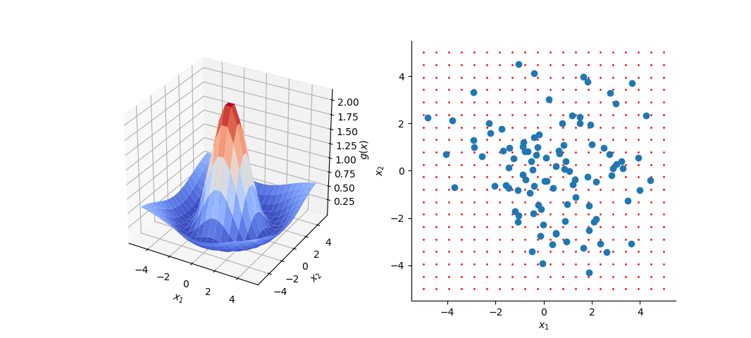
Figure 7: Left: Plot of the function ($d=2$). Right: A realisation of the data generation with $n=100$ (blue points). The red points are the locations of the testing data.

Table 6 presents a summary of the results obtained over 20 independent replications. The inference is based on 10,000 iterations with the first 5,000 iterations discarded as the burn-in period for both the unconstrained (UNCONS) and the constrained (CONS) models. For the $n=100$ case, both models give fairly good estimates for $\sigma^{2}$ (true $\sigma^{2}=0.25$), with relatively low IACT, indicating the good mixture behaviour of the chain. The RMSE for the training data are close for both models. For the test data, CONS generates better prediction results with lower RMSE. The raw predictions do not take the non-negative constraint into consideration. The correction rounds up the negative predictions to zero for UNCONS. For CONS, the posterior prediction distribution is a constrained truncated normal distribution. We use the posterior median as it is more robust than the posterior mean. Section E.3 gives more details. The corrected predictions of CONS reduce RMSE by around 25% compared with UNCONS.

For the large dataset $n=1{,}000$, the $\mathcal{GP}$ is placed on the inducing points (50 observations). Similarly to the previous results, the performance of CONS and UNCONS is close in terms of IACT and RMSE for the training data. For the test data predictions, CONS has 30-40% lower RMSE compared to UNCONS. The larger gap can be explained because the predictions are mainly based on the inducing points, not the whole dataset, resulting in less support from the neighbouring points. Consequently, the extrapolation based on an inducing point with a negative value is likely to yield a negative prediction. For UNCONS, such extrapolation amplifies the prediction error given the constraint is not incorporated into the model.

Other methods such as modelling $\mathbf{g}$ as a latent variable cannot be applied directly to this problem because it is difficult to sample $\mathbf{g}$ from a high-dimensional truncated multivariate normal distribution. The SOV estimator can help to generate $\mathbf{g}$, but the method is likely to fail in the high-dimensional space. Similarly, it is also not applicable to implement the exchange algorithm in Section 4.1.

$n=100$
				RMSE
Method	$d$	$\sigma^{2}$	IACT	train	test-raw	test-corrected
UNCONS	2	0.235	11.088	0.180	0.284	0.232
		(0.008)	(0.240)	(0.008)	(0.011)	(0.008)
CONS	2	0.259	11.371	0.178	0.212	0.179
		(0.009)	(0.198)	(0.008)	(0.008)	(0.008)
UNCONS	4	0.229	16.647	0.272	0.495	0.486
		(0.015)	(1.972)	(0.010)	(0.010)	(0.009)
CONS	4	0.308	14.012	0.256	0.488	0.371
		(0.010)	(0.527)	(0.006)	(0.003)	(0.009)
$n=1{,}000$
				RMSE
Method	$d$	$\sigma^{2}$	IACT	train	test-raw	test-corrected
UNCONS	2	0.237	10.26	0.076	0.143	0.132
		(0.002)	(0.279)	(0.003)	(0.006)	(0.004)
CONS	2	0.237	10.055	0.070	0.122	0.094
		(0.002)	(0.247)	(0.002)	(0.003)	(0.002)
UNCONS	4	0.204	12.157	0.203	0.468	0.463
		(0.005)	(0.464)	(0.004)	(0.002)	(0.002)
CONS	4	0.216	11.848	0.205	0.461	0.275
		(0.006)	(0.371)	(0.005)	(0.001)	(0.003)

Table 6: Results for the $\mathcal{GP}$ prior using observations of sizes 100 and 1,000. The results obtained are the mean value of 20 independent replications with the standard error in brackets. For the large dataset ($n=1{,}000$), 50 inducing points are used. “CONS” and “UNCONS” stand for the model with/without constraints (no intractable quantity involved). The negative predictions are rounded up to zero for both models. The lower value of RMSE in each category (train, test-raw, test-corrected) is highlighted in boldface. The “test-raw” shows the unmodified prediction result and the “test-corrected” rounds up the negative prediction to zero.

E.3 Prediction based on the constrained GP

Obtaining “raw” predictions follows the same procedure as an ordinary $\mathcal{GP}$ without constraints. The results are established in Williams and Rasmussen, (2006) and Snelson and Ghahramani, (2006) for scalable $\mathcal{GP}$. We illustrate the posterior prediction under the constraint below.

Prediction at $\mathbf{x}$: Denote $g(\mathbf{x})$ as $\mathbf{g}$ and $\boldsymbol{\theta}:=(\alpha,\rho,\sigma)$. To get the prediction for $\mathbf{g}$ for the small data case, consider the expectation with respect to the posterior distribution,

$$E(\mathbf{g}|\mathbf{y}) =\int_{\mathbf{g}}\mathbf{g}p(\mathbf{g}|\mathbf{y})d\mathbf{g}$$

$$=\int_{\mathbf{g}}\mathbf{g}\left(\int_{\boldsymbol{\theta}}p(\mathbf{g}|\boldsymbol{\theta},\mathbf{y})p(\boldsymbol{\theta}|\mathbf{y})d\boldsymbol{\theta}\right)d\mathbf{g}$$

$$=\int_{\boldsymbol{\theta}}\int_{\mathbf{g}}\mathbf{g}p(\mathbf{g}|\boldsymbol{\theta},\mathbf{y})p(\boldsymbol{\theta}|\mathbf{y})d\mathbf{g}d\boldsymbol{\theta},$$

where $p(\mathbf{g}|\boldsymbol{\theta},\mathbf{y})$ is a truncated multivariate normal distribution with mean $\boldsymbol{\mu}_{g}^{*}$, covariance $\boldsymbol{\Sigma}_{g}^{*},$ with the lower bound 0. The expressions for $\boldsymbol{\mu}_{g}^{*},\boldsymbol{\Sigma}_{g}^{*}$ follow the notation used in Sections E.2 and E.2.1. There is no extra computing cost because samples of $\mathbf{g}$ are obtained in the process of evaluating $\widehat{Z^{*}}(\boldsymbol{\theta})$ in the MCMC iterations.

For the scalable $\mathcal{GP}$, $\boldsymbol{\mu}_{g}^{*}$ and $\boldsymbol{\Sigma}_{g}^{*}$ are replaced with or $\boldsymbol{\mu}_{\overline{g}}^{*}$ and $\boldsymbol{\Sigma}_{\overline{g}}^{*}$. The samples of $\overline{\mathbf{g}}$ need to be further projected to the location $\mathbf{x}$ by $\overline{g}_{m}(\mathbf{x})=\mathbf{K}_{nm}\mathbf{K}^{-1}_{mm}\overline{\mathbf{g}}_{m}$.

Prediction at $\mathbf{x}^{*}$: Starting with the small sample case first, to predict $g^{*}(\mathbf{x}^{*})$ at a new location $\mathbf{x}^{*}$, we have:

$$E(\mathbf{g}^{*}|\mathbf{y}) =\int\mathbf{g}^{*}p(\mathbf{g}^{*}|\mathbf{y})d\mathbf{g}^{*}$$

$$=\int_{\mathbf{g}^{*}}\mathbf{g}^{*}\int_{\mathbf{g}}\int_{\boldsymbol{\theta}}p(\mathbf{g}^{*}|\mathbf{g},\mathbf{y},\boldsymbol{\theta})p(\mathbf{g}|\boldsymbol{\theta},\mathbf{y})p(\boldsymbol{\theta}|\mathbf{y})d\mathbf{g}d\boldsymbol{\theta}d\mathbf{g}^{*}$$

$$=\int_{\mathbf{g}^{*}}\int_{\mathbf{g}}\int_{\boldsymbol{\theta}}\mathbf{g}^{*}p(\mathbf{g}^{*}|\mathbf{g},\boldsymbol{\theta})p(\mathbf{g}|\boldsymbol{\theta},\mathbf{y})p(\boldsymbol{\theta}|\mathbf{y})d\mathbf{g}d\boldsymbol{\theta}d\mathbf{g}^{*},$$

where $p(\mathbf{g}^{*}|\mathbf{g},\boldsymbol{\theta})=\textrm{trunc{-}normal}(\mathbf{g}^{*}|\boldsymbol{\mu}_{g^{*}|g},\boldsymbol{\Sigma}_{g^{*}|g};\mathbf{0},\boldsymbol{\infty})$ with $\boldsymbol{\mu}_{g^{*}|g}=\mathbf{K}_{x^{*}x}\mathbf{K}^{-1}_{xx}\mathbf{g}$ and $\boldsymbol{\Sigma}_{g^{*}|g}=\mathbf{K}_{x^{*}x}-\mathbf{K}_{x^{*}x}\mathbf{K}^{-1}_{xx}\mathbf{K}_{xx^{*}}$. It is expensive to sample a vector $\mathbf{g}^{*}$ from $p(\mathbf{g}^{*}|\mathbf{g},\boldsymbol{\theta})$ as it requires $O(n_{pred}^{3})$ evaluations to get the Cholesky decomposition of the matrix $\boldsymbol{\Sigma}_{g^{*}|g}$. Here $n_{pred}$ refers to the number of observations for prediction. Instead, consider a one-dimensional $\mathbf{g}^{*}$ so that $p(\mathbf{g}^{*}|\mathbf{g},\boldsymbol{\theta})$ is reduced to a one-dimensional truncated normal distribution with a known normalising constant. The analytical forms of quantities such as the mean and median of one-dimensional truncated normal distributions are available. In the simulation study, the median is selected as it is more robust than the mean.

For the scalable $\mathcal{GP}$, $p(\mathbf{g}^{*}|\mathbf{g},\boldsymbol{\theta})$ is a truncated normal distribution with mean vector $\boldsymbol{\mu}_{g^{*}|\overline{g}_{m}}=\mathbf{K}_{x^{*}m}\mathbf{K}^{-1}_{mm}\overline{\mathbf{g}}_{m}$ and the variance $\mathbf{K}_{x^{*}x^{*}}(\mathbf{K}^{-1}_{mm}-\mathbf{Q}_{mm}^{-1})\mathbf{K}_{xx^{*}}$.

References

- Andrieu and Roberts, (2009) Andrieu, C. and Roberts, G. O. (2009). The pseudo-marginal approach for efficient Monte Carlo computations. The Annals of Statistics, 37(2):697–725.
- Andrieu and Vihola, (2016) Andrieu, C. and Vihola, M. (2016). Establishing some order amongst exact approximations of MCMCs. The Annals of Applied Probability, 26(5):2661–2696.
- Atchadé et al., (2013) Atchadé, Y. F., Lartillot, N., and Robert, C. (2013). Bayesian computation for statistical models with intractable normalizing constants. Brazilian Journal of Probability and Statistics, 27(4):416–436.
- Beaumont, (2003) Beaumont, M. A. (2003). Estimation of population growth or decline in genetically monitored populations. Genetics, 164(3):1139–1160.
- Betancourt, (2020) Betancourt, M. (2020). Robust Gaussian process modeling. https://github.com/betanalpha/knitr_case_studies/tree/master/gaussian_processes/gaussian_processes.html.
- Brooks et al., (2011) Brooks, S., Gelman, A., Jones, G., and Meng, X.-L. (2011). Handbook of Markov Chain Monte Carlo. CRC press.
- Cai and Adams, (2022) Cai, D. and Adams, R. P. (2022). Multi-fidelity Monte Carlo: A pseudo-marginal approach. Advances in Neural Information Processing Systems.
- Carter and Cashwell, (1975) Carter, L. L. and Cashwell, E. D. (1975). Particle-transport simulation with the Monte Carlo method. Technical report, Los Alamos Scientific Lab., N. Mex.(USA).
- Ceperley and Dewing, (1999) Ceperley, D. and Dewing, M. (1999). The penalty method for random walks with uncertain energies. The Journal of Chemical Physics, 110(20):9812–9820.
- Deligiannidis et al., (2018) Deligiannidis, G., Doucet, A., and Pitt, M. K. (2018). The correlated pseudomarginal method. Journal of the Royal Statistical Society: Series B (Statistical Methodology), 80(5):839–870.
- Dowe et al., (1996) Dowe, D. L., Oliver, J. J., and Wallace, C. S. (1996). MML estimation of the parameters of the spherical fisher distribution. In International Workshop on Algorithmic Learning Theory, pages 213–227. Springer.
- Efron, (1992) Efron, B. (1992). Bootstrap methods: Another look at the jackknife. In Breakthroughs in Statistics, pages 569–593. Springer.
- Figueiredo, (2009) Figueiredo, A. (2009). Discriminant analysis for the von Mises-Fisher distribution. Communications in Statistics-Simulation and Computation, 38(9):1991–2003.
- Fisher et al., (1993) Fisher, N. I., Lewis, T., and Embleton, B. J. (1993). Statistical Analysis of Spherical Data. Cambridge University Press.
- Fredrickson and Andersen, (1984) Fredrickson, G. H. and Andersen, H. C. (1984). Kinetic Ising model of the glass transition. Physical Review Letters, 53(13):1244.
- Garthwaite et al., (2016) Garthwaite, P. H., Fan, Y., and Sisson, S. A. (2016). Adaptive optimal scaling of Metropolis–Hastings algorithms using the Robbins–Monro process. Communications in Statistics-Theory and Methods, 45(17):5098–5111.
- Genz, (1992) Genz, A. (1992). Numerical computation of multivariate normal probabilities. Journal of Computational and Graphical Statistics, 1(2):141–149.
- Hastings, (1970) Hastings, W. K. (1970). Monte Carlo sampling methods using Markov chains and their applications. Biometrika, 57(1):97–109.
- Herrero, (2002) Herrero, C. P. (2002). Ising model in small-world networks. Physical Review E, 65(6):066110.
- Hughes et al., (2011) Hughes, J., Haran, M., and Caragea, P. C. (2011). Autologistic models for binary data on a lattice. Environmetrics, 22(7):857–871.
- Hunter and Handcock, (2006) Hunter, D. R. and Handcock, M. S. (2006). Inference in curved exponential family models for networks. Journal of Computational and Graphical Statistics, 15(3):565–583.
- Ising, (1925) Ising, E. (1925). Beitrag zur theorie des ferromagnetismus. Zeitschrift für Physik, 31(1):253–258.
- Jacob and Thiery, (2015) Jacob, P. E. and Thiery, A. H. (2015). On nonnegative unbiased estimators. The Annals of Statistics, 43(2):769–784.
- Kasarapu, (2015) Kasarapu, P. (2015). Modelling of directional data using Kent distributions. arXiv preprint arXiv:1506.08105.
- Kent, (1982) Kent, J. T. (1982). The Fisher-Bingham distribution on the sphere. Journal of the Royal Statistical Society: Series B (Methodological), 44(1):71–80.
- Kent et al., (2013) Kent, J. T., Ganeiber, A. M., and Mardia, K. V. (2013). A new method to simulate the Bingham and related distributions in directional data analysis with applications. arXiv preprint arXiv:1310.8110.
- Kolmogorov and Zabin, (2004) Kolmogorov, V. and Zabin, R. (2004). What energy functions can be minimized via graph cuts? IEEE Transactions on Pattern Analysis and Machine Intelligence, 26(2):147–159.
- Kume and Wood, (2005) Kume, A. and Wood, A. T. (2005). Saddlepoint approximations for the Bingham and Fisher–Bingham normalising constants. Biometrika, 92(2):465–476.
- Lenz, (1920) Lenz, W. (1920). Beitršge zum verstšndnis der magnetischen eigenschaften in festen kšrpern. Physikalische Z, 21:613–615.
- Liang, (2010) Liang, F. (2010). A double Metropolis–Hastings sampler for spatial models with intractable normalizing constants. Journal of Statistical Computation and Simulation, 80(9):1007–1022.
- Liang et al., (2016) Liang, F., Jin, I. H., Song, Q., and Liu, J. S. (2016). An adaptive exchange algorithm for sampling from distributions with intractable normalizing constants. Journal of the American Statistical Association, 111(513):377–393.
- Liu et al., (2020) Liu, H., Ong, Y.-S., Shen, X., and Cai, J. (2020). When Gaussian process meets big data: A review of scalable GPS. IEEE Transactions on Neural Networks and Learning Systems, 31(11):4405–4423.
- Lyne et al., (2015) Lyne, A.-M., Girolami, M., Atchadé, Y., Strathmann, H., Simpson, D., et al. (2015). On Russian roulette estimates for Bayesian inference with doubly-intractable likelihoods. Statistical Science, 30(4):443–467.
- Metropolis et al., (1953) Metropolis, N., Rosenbluth, A. W., Rosenbluth, M. N., Teller, A. H., and Teller, E. (1953). Equation of state calculations by fast computing machines. The Journal of Chemical Physics, 21(6):1087–1092.
- Møller et al., (2006) Møller, J., Pettitt, A. N., Reeves, R., and Berthelsen, K. K. (2006). An efficient Markov chain Monte Carlo method for distributions with intractable normalising constants. Biometrika, 93(2):451–458.
- Murray et al., (2006) Murray, I., Ghahramani, Z., and MacKay, D. J. C. (2006). MCMC for doubly-intractable distributions. In Proceedings of the Twenty-Second Conference on Uncertainty in Artificial Intelligence, UAI’06, page 359–366, Arlington, Virginia, USA. AUAI Press.
- Murray and Graham, (2016) Murray, I. and Graham, M. (2016). Pseudo-marginal slice sampling. In Artificial Intelligence and Statistics, pages 911–919. PMLR.
- Neal, (2001) Neal, R. M. (2001). Annealed importance sampling. Statistics and Computing, 11(2):125–139.
- Papaspiliopoulos, (2011) Papaspiliopoulos, O. (2011). Monte Carlo probabilistic inference for diffusion processes: A methodological framework. Bayesian Time Series Models, pages 82–103.
- Park and Haran, (2018) Park, J. and Haran, M. (2018). Bayesian inference in the presence of intractable normalizing functions. Journal of the American Statistical Association, 113(523):1372–1390.
- Pitt et al., (2012) Pitt, M. K., dos Santos Silva, R., Giordani, P., and Kohn, R. (2012). On some properties of Markov chain Monte Carlo simulation methods based on the particle filter. Journal of Econometrics, 171(2):134–151.
- Propp and Wilson, (1996) Propp, J. G. and Wilson, D. B. (1996). Exact sampling with coupled Markov chains and applications to statistical mechanics. Random Structures & Algorithms, 9(1-2):223–252.
- Quinonero-Candela and Rasmussen, (2005) Quinonero-Candela, J. and Rasmussen, C. E. (2005). A unifying view of sparse approximate Gaussian process regression. The Journal of Machine Learning Research, 6:1939–1959.
- Quiroz et al., (2019) Quiroz, M., Kohn, R., Villani, M., and Tran, M.-N. (2019). Speeding up MCMC by efficient data subsampling. Journal of the American Statistical Association, 114(526):831–843.
- Quiroz et al., (2021) Quiroz, M., Tran, M.-N., Villani, M., Kohn, R., and Dang, K.-D. (2021). The block-Poisson estimator for optimally tuned exact subsampling MCMC. Journal of Computational and Graphical Statistics, 30(4):877–888.
- Rossi et al., (2021) Rossi, S., Heinonen, M., Bonilla, E., Shen, Z., and Filippone, M. (2021). Sparse Gaussian processes revisited: Bayesian approaches to inducing-variable approximations. In International Conference on Artificial Intelligence and Statistics, pages 1837–1845. PMLR.
- Schmidt, (1976) Schmidt, P. (1976). The non-uniqueness of the Australian Mesozoic palaeomagnetic pole position. Geophysical Journal International, 47(2):285–300.
- Seeger et al., (2003) Seeger, M. W., Williams, C. K., and Lawrence, N. D. (2003). Fast forward selection to speed up sparse Gaussian process regression. In International Workshop on Artificial Intelligence and Statistics, pages 254–261. PMLR.
- Snelson and Ghahramani, (2006) Snelson, E. and Ghahramani, Z. (2006). Sparse Gaussian processes using pseudo-inputs. Advances in Neural Information Processing Systems, 18:1257.
- Swiler et al., (2020) Swiler, L. P., Gulian, M., Frankel, A. L., Safta, C., and Jakeman, J. D. (2020). A survey of constrained Gaussian process regression: Approaches and implementation challenges. Journal of Machine Learning for Modeling and Computing, 1(2).
- Tran et al., (2016) Tran, M.-N., Kohn, R., Quiroz, M., and Villani, M. (2016). The block pseudo-marginal sampler. arXiv preprint arXiv:1603.02485.
- Wei and Murray, (2017) Wei, C. and Murray, I. (2017). Markov chain truncation for doubly-intractable inference. In Artificial Intelligence and Statistics, pages 776–784. PMLR.
- Williams and Rasmussen, (2006) Williams, C. K. and Rasmussen, C. E. (2006). Gaussian Processes for Machine Learning, volume 2. MIT Press Cambridge, MA.
- Wood, (1982) Wood, A. (1982). A bimodal distribution on the sphere. Journal of the Royal Statistical Society: Series C (Applied Statistics), 31(1):52–58.