Domain Generalization via Contrastive Causal Learning

Abstract

Domain Generalization (DG) aims to learn a model that can generalize well to unseen target domains from a set of source domains. With the idea of invariant causal mechanism, a lot of efforts have been put into learning robust causal effects which are determined by the object yet insensitive to the domain changes. Despite the invariance of causal effects, they are difficult to be quantified and optimized. Inspired by the ability that humans adapt to new environments by prior knowledge, We develop a novel Contrastive Causal Model (CCM) to transfer unseen images to taught knowledge which are the features of seen images, and quantify the causal effects based on taught knowledge. Considering the transfer is affected by domain shifts in DG, we propose a more inclusive causal graph to describe DG task. Based on this causal graph, CCM controls the domain factor to cut off excess causal paths and uses the remaining part to calculate the causal effects of images to labels via the front-door criterion. Specifically, CCM is composed of three components: (i) domain-conditioned supervised learning which teaches CCM the correlation between images and labels, (ii) causal effect learning which helps CCM measure the true causal effects of images to labels, (iii) contrastive similarity learning which clusters the features of images that belong to the same class and provides the quantification of similarity. Finally, we test the performance of CCM on multiple datasets including PACS, OfficeHome, and TerraIncognita. The extensive experiments demonstrate that CCM surpasses the previous DG methods with clear margins.

Introduction

Humans have the ability to solve specific problems with the help of previous knowledge. This generalization capability helps humans take advantage of stable causal effects to adapt to the environment shift. While deep learning has achieved great success in a wide range of real-world applications, due to the lack of out-of-distribution (OOD) generalization ability (Krueger et al. 2021; Sun et al. 2020; Zhang et al. 2021), it suffers from a catastrophic performance degradation problem, especially when deployed in new environments with changing distributions. Although Domain Adaptation (DA) algorithms (Fu et al. 2021; Li et al. 2021b, c, d) support models to adapt to various target domains, different target domains need corresponding domain adaptation processes. In order to deal with domain shift problems, Domain Generalization (DG) (Zhang et al. 2021; Chen et al. 2021; Liu et al. 2021; Sun et al. 2021; Mahajan, Tople, and Sharma 2021; Wald et al. 2021) is introduced, which aims to learn stable knowledge from multiple source domains and train a generalizable model directly to unseen target domains.

Increasing works on DG have been proposed with a variety of strategies like data augmentation (Carlucci et al. 2019; Wang et al. 2020; Zhou et al. 2020b, a, 2021), meta-learning (Balaji, Sankaranarayanan, and Chellappa 2018; Li et al. 2018a; Dou et al. 2019; Li et al. 2019a, b), invariant representation learning (Zhao et al. 2020; Matsuura and Harada 2020; Li et al. 2018d, c), et al. While promising performance has been achieved by these methods, they might try to model the statistical dependence between the input features and the labels, hence could be biased by the spurious correlation in data (Liu et al. 2021). With the idea of invariant causal mechanism, increasing attention has been paid to causality-inspired generalization learning (Wald et al. 2021; Liu et al. 2021; Sun et al. 2021; Mahajan, Tople, and Sharma 2021). For example, Liu et al. (Liu et al. 2021) introduce their causal semantic generative model to learn semantic factors and variation factors separately via variational Bayesian. Sun et al. (Sun et al. 2021) further introduce a domain variable and an unobserved confounder to describe a latent causal invariant model. Mahajan et al. (Mahajan, Tople, and Sharma 2021) consider high-level causal features and domain-dependent features while the labels are only determined by the former. Each of the casual graphs given by them has a different focus, but there are commonalities among them.

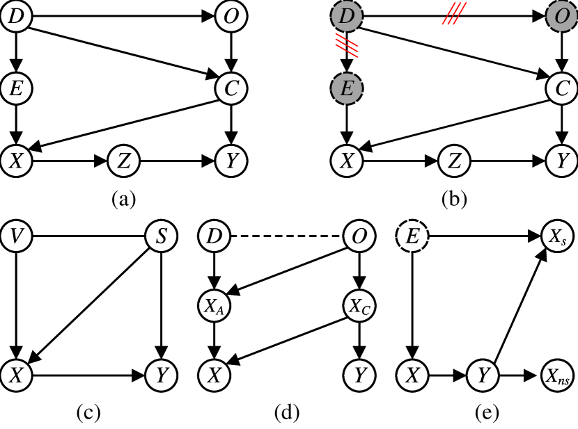
Figure 1: Comparisons between the causal graphs of CCM (a), (b) and the previous methods (c) (Liu et al. 2021; Sun et al. 2021), (d) (Mahajan, Tople, and Sharma 2021), and (e) (Wald et al. 2021). In Figure (a), based on Figure (c), Figure (d), and Figure (e), we add prior knowledge $Z$ as a bridge to link unseen image $X$ and label $Y$ and make domain $D$ point to object $O$ and category factor $C$ to explain the limitations of source domain on models in DG. In Figure (b), by controlling domain $D$, the remaining part is a standard causal graph that can calculate causal effects from $X$ to $Y$ via the front-door criterion.

In this paper, we propose a causal graph to formalize the DG problem from a novel perspective as shown in Figure 1 (a) and Figure 1 (b). To create a data sample in a certain environment, e.g., an image of a polar bear in the Arctic and the corresponding label of the bear, We can guess from the domain $D$ of the image that the object $O$ is a hardy animal (i.e. $D\rightarrow O$). The hardy animal that lives in the Arctic may be the polar bear (i.e. $D\rightarrow C\leftarrow O$). The domain factor not only affects object $O$ and category $C$, but also provides background features $E$ to the image $X$ (i.e. $D\rightarrow E\rightarrow X$). Combining the dual information of background $E$ and category $C$, the image $X$ is captured and transformed into prior knowledge (e.g. the seen images of brown bears) to predict its label $Y$ (i.e. $X\rightarrow Z\rightarrow Y$). And the label $Y$ is determined based on the match between knowledge $Z$ and category $C$. Compared to Figure 1 (c), Figure 1 (d) and Figure 1 (e), we add prior knowledge $Z$ as a bridge to link unseen image $X$ and label $Y$. The the relationships between domain $D$ and other factors can be explained more clearly by figure 1 (b). In Figure 1 (a), the domain $D$ as a confounder disturbs models to learn causal effects from image $X$ to labels $Y$. So we control domain $D$ to cut off $D\rightarrow O$ and $D\rightarrow E$, and the remaining part is a standard causal graph that can calculate causal effects from $X$ to $Y$ via the front-door criterion, as shown in Figure 1 (b).

To learn the causal effects of $X$ to $Y$ shown in Figure 1 (b), we introduce the front-door criterion. It splits the causal effects of $P(Y|do(X))$ into the estimation of three parts: $P(X)$, $P(Z|X)$, and $P(Y|Z,X)$. Furthermore, to permit stable distribution estimation under causal learning, we further design a contrastive training paradigm that calibrates the learning process with the similarity of the current and previous knowledge to strengthen true causal effects.

Our main contributions are summarized as follows. (i) We develop a Contrastive Causal Model to transfer unseen images into taught knowledge that, and quantify the causal effects between images and labels based on taught knowledge. (ii) We propose an inclusive causal graph that can explain the inference of domain in the DG task. Based on this graph, our model cuts off the excess causal paths and quantifies the causal effects between images and labels via the front-door criterion. (iii) Extensive experiments on public benchmark datasets demonstrate the effectiveness and superiority of our method.

Related Work

Domain Generalization

Domain generalization (DG) aims to learn from multiple source domains a model that can perform well on unseen target domains. Data augmentation-based methods (Volpi et al. 2018; Shankar et al. 2018; Carlucci et al. 2019; Wang et al. 2020; Zhou et al. 2020b, a, 2021) try to improve the generalization robustness of the model by learning from the data with novel distributions. Among them, some work (Volpi et al. 2018; Shankar et al. 2018) generates new data based on model gradient and leverages it to train a model for boosting its robustness. While others (Wang et al. 2020; Carlucci et al. 2019) introduce an interesting jigsaw puzzle strategy that improves model out-of-distribution generalization via self-supervised learning. Adversarial training (Zhou et al. 2020b, a) is also employed to generate data with various styles yet consistent semantic information. Meta-learning (Balaji, Sankaranarayanan, and Chellappa 2018; Li et al. 2018a; Dou et al. 2019; Li et al. 2019a, b) is also a popular topic in DG. The idea is similar to the problem setting of DG: learning from the known and preparing for inference from the unknown. However, it might not be easy to design effective meta-learning strategies for training a generalizable model. Another conventional direction is to perform invariant representation learning (Zhao et al. 2020; Matsuura and Harada 2020; Li et al. 2018d, c). These methods try to learn the feature representations that are discriminative for the classification task but invariant to the domain changes. For example, (Zhao et al. 2020) proposes conditional entropy regularization to extract effective conditional invariant feature representations. While favorable results have been achieved by these approaches, they might try to model the statistical dependence between the input features and the labels, hence could be biased by the spurious correlation (Liu et al. 2021).

Domain Generalization with Causality

In this paper, we assume the data is generated from the root factors of the object $O$ and domain $D$ as shown in Figure 1 (a). The class features $C$ control both the input feature $X$ and the label $Y$, meanwhile, the environment feature $E$ only affects $X$. We aim to learn an informative representation from $X$ to predict $Y$. (Liu et al. 2021) proposes a causal semantic generative model (see Figure 1 (c)). It separates the latent semantic factor $S$ and variation factor $V$ from data, where only the former causes the change in label $Y$. Similarly, (Sun et al. 2021) introduces latent causal invariant models based on the same causal model structure. Their semantic factor $S$ and variation factor $V$ are similar to the class feature $C$ and the environment feature $E$ in our causal graph respectively, while we further show their causal relationship with domain and object. (Mahajan, Tople, and Sharma 2021) proposes a causal graph with the domain $D$ and object $O$ which is similar to ours, as shown in Figure 1 (d). It assumes that the input feature $X$ is determined by causal feature $X_{C}$ and domain-dependent feature $X_{A}$, and the label $Y$ is determined by $X_{C}$. Actually, the representation $Z$ (Figure 1 (a)) that we aim to learn is to capture the information of causal feature $X_{C}$ (Figure 1 (d)). (Wald et al. 2021) puts forward model calibration for the source domains based on the graph in Figure 1 (e). It splits the information in the label $Y$ into anti-causal spurious features $X_{s}$ and anti-causal non-spurious features $X_{ns}$, where the information of the latter is aimed to learn as the representation $Z$ in our causal graph. Therefore, our proposed causal graph can be seen as a uniform structure of the previous methods and is generally compatible with the structure of the previous works.

Contrastive Learning

Recently, contrastive learning (Wang and Liu 2021; Chen and He 2021; Chen et al. 2020; He et al. 2020) as an unsupervised learning paradigm has drawn increasing attention due to its excellent representation learning ability. The goal of contrastive learning is to gather similar samples and diverse samples that are far from each other. For example, (He et al. 2020) introduces the popular MoCo framework, which builds dynamic dictionaries and learns the representations based on a contrastive loss.

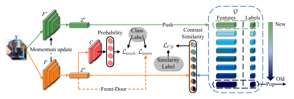
Figure 2: The framework of CCM. The teacher $F$ and student $F^{\prime}$ have the same structure, and the student $F^{\prime}$ gets experiences from teacher $F$ by momentum update. The teacher $F$ extract the features $Z^{k}$ of images $X^{k}$ and send them to classifier $C$ to calculate $\mathcal{L}_{teach}$. The features $Z^{k}$ are also used to calculate $\mathcal{L}_{learn}$ via the front-door criterion with knowledge queue $Q$. To quantify the causal effect more accurately, we measure the contrastive similarity between features $Z^{k}$ and the features in the knowledge queue $Q$. And optimizing $\mathcal{L}_{CS}$ can cluster the features with the same category. Finally, the student $F^{\prime}$ obtain historical features $Z^{\prime}$ and pushes them into the knowledge queue $Q$. The oldest features and their labels in the knowledge queue $Q$ are popped.

Proposed Method

To introduce CCM more clearly, we give some necessary notations first. We donate the joint space of the input image and the label as $\mathcal{X}\times\mathcal{Y}$. There are $k$ source domains with different statistical distributions defined on the joint space. The $k$th source domain is $D_{k}=\{(x_{i}^{k},y_{i}^{k})\}_{i=1}^{N_{k}}$. The teacher $F$ and student $F^{\prime}$ are two backbones with the same structure. The features of images are defined as $Z$. CCM has a classifier $C$ and a knowledge queue $Q$, which stores features and labels.

The Contrastive Causal Model (CCM) addresses the domain generalization problem by introducing contrastive similarity to convert new images to previous knowledge and increase the percentage of causal effects from images to labels with the help of the front-door criterion. In the following, we introduce the structural causal model of CCM first. And then, we introduce the structure of CCM specifically from three main parts: domain-conditioned supervised learning, causal effect learning, and contrastive similarity learning.

Structural Causal Model of CCM

There is a series of prior works (Christiansen et al. 2021; Yuan et al. 2021; Mahajan, Tople, and Sharma 2021; Chen et al. 2021; Sun et al. 2021; Li et al. 2021a) investigate domain generalization task and provide their own approaches in causal view. While these methods strengthen the causal effects between images to labels, the spurious correlation given by domain does not get enough attention. Using the structural causal model (SCM) can explain this weakness obviously. In (Christiansen et al. 2021; Yuan et al. 2021), their SCMs show the direct causal path from image $X$ to label $Y$. However, (Christiansen et al. 2021) ignores the intermediate product $Z$ of the feature extractor and classifier. (Yuan et al. 2021) regard $Z$ as domain-invariant relationship. In our SCM, the causal path $X\rightarrow Z\rightarrow Y$ implies extracting true causal features $Z$ from image $X$ by feature extractor $F$ and predicting the label $Y$ based on $Z$ by classifier $C$. In addition, several recent works(Mahajan, Tople, and Sharma 2021; Chen et al. 2021; Sun et al. 2021; Li et al. 2021a) have further identified other hidden causal relationship. These works introduce domain variable $D$. $D$ determines the domain identity $E$ which independent of category information, representing in Fig 1(a) as $D\rightarrow E$. Especially in works(Li et al. 2021a; Mahajan, Tople, and Sharma 2021; Chen et al. 2021), these SCMs introduce variables that are only relevant to objects. Like the path from object $O$ to category factor $C$. By mixing the object factor and domain factor, the image $X$ is generated by causal path $E\rightarrow X\leftarrow C$. But in a fixed domain, $D$ also influence $O$ and $C$. For example, we can speculate about the presence of the bear object based on the information that the location is the North Pole. But the location cannot be inferred to be the North Pole based solely on the presence of the bear object. So we add the path $D\leftarrow O$. Along these lines, the Arctic environment and the presence of bear targets led to a more refined category factor of polar bears rather than black bears. So it has a path from $D$ to $C$. The SCMs proposed by previous works are organized as Fig 1(a).

In Fig 1 (a), there four causal effect paths from image $X$ to label $Y$: (i) $X\rightarrow Z\rightarrow Y$, (ii) $X\leftarrow C\rightarrow Y$, (iii) $X\leftarrow E\leftarrow D\rightarrow C\rightarrow Y$, (iv) $X\leftarrow E\leftarrow D\rightarrow O\rightarrow C\rightarrow Y$. Path $X\rightarrow Z\rightarrow Y$ is the main causal effect path. If other paths do not exist, using path $X\rightarrow Z\rightarrow Y$ can learn the pure causal relationship between $X$ to $Y$. So how cutting off the excess path is important. In Fig 1 (b), we control domain factor $D$ to cut off $D\rightarrow E$ and $D\rightarrow O$ (i.e. cut off $X\leftarrow E\leftarrow D\rightarrow C\rightarrow Y$ and $X\leftarrow E\leftarrow D\rightarrow O\rightarrow C\rightarrow Y$). This operation is equivalent to slicing the source domain data for different sub-domains. Furthermore, with the change of images, only the category factor $O$ disturbs models to learn causal effects of $X\rightarrow Z\rightarrow Y$ in the fixed domain. Due to the severance of the causal paths, the category factor $C$ is a confounder of $X$ and $Y$ on the remaining causal graph and is suitable to use the front-door criterion to remove its interference.

Domain-Conditioned Supervised Learning

Conventional supervised learning directly minimizes the empirical risk of the training data to learn the relationship between the features of images and labels. Here, we fix the domain factor to cut off the confounding effect of the domain as shown in Figure 1 (b). Thus, it turns out to be domain-conditioned supervised learning. And we minimize the cross-entropy loss conditioned on the domain for supervised learning. That is,

$$\mathcal{L}_{teach}^{D_{k}}=-\frac{1}{N_{k}}\sum_{i=1}^{N_{k}}y_{i}^{D_{k}}\textrm{log}C(F(x_{i}^{D_{j}}))$$ (1)

The teaching $\mathcal{L}_{teach}$ helps CCM learn the correlation of image to label across different domains, which contain causal effects from image $X$ to label $Y$. In other words, casual effects are parts of the correlation. If the model only allows using causal effects for inference without teaching it the correlation between image and label, the task will be too difficult for a model to solve. This point is verified in our ablation experiments.

Causal Effect Learning

After teaching the model about correlation, we desire to measure how much CCM learns the causal effects between the input and the label. Here, we introduce the front-door criterion to measure the causal effects and increase the percentage of them via $do(\cdot)$ operation:

$$P(Y|do(X))$$ (2)

$$= \sum_{z}P(Z=z|X)$$

$$\sum_{x}[P(X=x)P(Y=y|Z=z,X=x)]$$

Take CCM as an example, $X$ is the set of images, and $Y$ is the set containing their corresponding labels. Moreover, $Z$ is the prior knowledge learned by the images that the model has been taught. Specifically, the causal path $X\rightarrow Z\rightarrow Y$ means the model converts an unseen image to prior knowledge and predicts its label. This behavior is consistent with the reflection of human adaptation to a new environment.

There are three main parts in $do(\cdot)$: $P(Z=z|X)$, $P(X=x)$ and $P(Y|Z=z,X=x)$. We will introduce them in order.

In $P(Z=z|X)$, $Z$ is a symbol of prior knowledge that has been taught. $Z$ is also an intermediary on the causal path from $X$ to $Y$. Inspired by recent work(He et al. 2020), we also construct a knowledge queue $Q$ to store trained features as prior knowledge to help CCM translate new images into learned knowledge. The feature set $Z^{Q}=\{z^{Q}_{1},z^{Q}_{2},\cdots,z^{Q}_{m}\}$ saved in $Q$ is a subset in feature space $\mathcal{Z}$ and is used for approximating the true distribution of $Z$ in space $\mathcal{Z}$. Not only the features set $Z^{Q}$ are stored in $Q$, but also its corresponding labels set $Y^{Q}=\{y^{Q}_{1},y^{Q}_{2},\cdots,y^{Q}_{m}\}$ is saved in $Q$. The effect of $Y^{Q}$ will be introduced specifically in the next section. After obtaining $X$, we define the contrastive similarity to calculate $P(Z=z|X)$ like Eq. 3.

$$M_{CS}(q,k)=\frac{\textrm{norm}(q)\cdot\textrm{norm}(k)^{T}}{\tau\cdot\sqrt{\textrm{d}}}$$ (3)

where $\tau$ is a temperature hyper-parameter and d the dimension of $q$ and $k$. $q$ and $k$ are two variables feeling in the model to measure contrastive similarity. More specifically, in Fig 2, we feed a batch of images $X$ of the domain $k$ into teacher $F$ to get corresponding features $Z^{k}$ first. Inspired by (He et al. 2020), there is a student $F^{\prime}$ which has the same structure as $F$ for obtaining historical features $Z^{\prime}$. The historical features $Z^{\prime}$ produced by student $F^{\prime}$ maintain consistency with $Z^{Q}$ with the help of momentum update from teacher $F$.

$$F^{\prime}=\alpha F^{\prime}+(1-\alpha)F$$ (4)

where $\alpha$ is the momentum ratio. It should be noticed that historical features $Z^{\prime}$ will be pushed in $Q$ after calculating loss to ensure CCM only use prior knowledge. Also the oldest feature $z_{m}^{Q}$ will be popped out to complete the update of knowledge queue $Q$. We set $Z^{k}$ as the agent of $X$ and use $Z^{k}$ and $Z^{Q}$ to calculate $P(Z=z|X)$. The $P(Z=z|X)$ is as follows:

$$P(Z=z_{i}^{Q}|X)=\textrm{norm}(\sum_{j=1}^{N}Softmax[M_{CS}(z_{i}^{Q},z_{j}^{k})])$$ (5)

In Eq. 5, we use L1 normalization to limit the range of output to get $P(Z=z|X)$.

To get $P(X=x)$, we should iterate all images in the real world, which is too hard to achieve. Therefore, we estimate the true distribution of $x$ in $\mathcal{X}$ by batch. It should be noticed that the images in a batch are chosen randomly, so we can measure $P(X=x)$ as $\frac{1}{N}$ directly, which $N$ is the batch size. However, this solution can not represent the relationship precisely between each image in one batch. For example, if there is an extremely similar image set $X_{sim}=\{x_{1},x_{1},\cdots,x_{n}\}$ in a batch, the probability of selecting any one of $X_{sim}$ should be $\frac{n}{N}$ instead of $\frac{1}{N}$. If the image $x$ is more similar to other images in the batch, it means that if the image $x$ is more common, then the corresponding $P(X=x)$ value is higher We put a batch of images $X$ into teacher $F$ to get a feature set $F(X)$, and then calculate the contrastive similarity between one feature $F(x)$ and features in the feature set $F(X)$ to get $P(X=x)$.

$$P(X=x)=Softmax[\sum_{i=1}^{N}M_{CS}(F(x),F(x_{i}))]$$ (6)

During the training process, we can get $P(X=x)$ by Eq. 6. In the inference phase, although the images are combined into a batch and fed into CCM, each image should be regarded as an individual that can not access any other images in this batch. So in the non-training period we set $P(X=x)=\frac{1}{N}$.

The $P(Y|Z=z,X=x)$ needs to iterate $z$ and $x$ as input to compute. Inspired by (Yang et al. 2021), we parameterize the predictive $P(Y|Z=z,X=x)$ as a model $G$. However, the $E$ of CCM in the implementation details is different. We regard $F(x)$ as the agent of $x$ and reduce the dimensions of $z$ and $F(x)$ to half of the original by model $H$ in order to align the dimensions of these two variables. Subsequently, both of them will be concatenated together as shown in Fig 2 and feed in $E$ to get $P(Y|Z=z,X=x)$ through the following equation:

$$\begin{split}&P(Y|Z=z,X=x)\\ =&Softmax[G(\textrm{concat}(H(z^{Q}),H(F(x))))]\end{split}$$ (7)

And now we can calculate Eq. 2 which represents the true causal effects from $X$ to $Y$ contained in the correlation. So we want to minimize $L_{learn}$ to increase the percentage of causal effects in the domain $D_{k}$ by the following equation:

$$\mathcal{L}_{learn}^{D_{k}}=-\frac{1}{N_{k}}\sum_{i=1}^{N_{k}}y_{i}^{D_{k}}\textrm{log}M_{FD}(x_{i}^{D_{k}})$$ (8)

where $M_{FD}(\cdot)$ is the symbol for the front-door adjustment formula.

Contrastive Similarity Learning

In Eq. 5 and Eq. 6, $M_{CS}(\cdot)$ is used several times for measure the similarity of two features. Although humans can distinguish which images contain objects in the same category, it is not straightforward to quantify the similarity of two images in the feature space $\mathcal{Z}$. In CCM, we propose Contrastive similarity learning to help the model obtain the ability to cluster the features of images that have the same class. After sending $X$ in $F^{\prime}$ to get feature set $Z^{\prime}$, we use $M_{CS}(\cdot)$ to measure the similarity of $Z^{\prime}$ and $Z^{Q}$. It should be noticed that the labels $Y^{Q}$ of $Z^{Q}$ are saved in $Q$. So, according to $Y$ and $Y^{Q}$, it can separate whether the features belong to the same class or not and get the binary labels $Y_{self}$. Subsequently, we minimize $L_{CS}$ to pull in the contrastive similarity of the features in the space $Z$.

$$\mathcal{L}_{CS}=-\frac{1}{N_{pair}}\sum_{i=1}^{N_{pair}}\textrm{log}M_{CS}({F}^{\prime}(x),z^{Q+}_{i})$$ (9)

where $z^{q+}_{i}$ are features in $Q$ that have the same labels of $x$, and $N_{pair}$ is the number of pairs $({F}^{\prime}(x),z^{Q+}_{i})$.

Overall

Finally, we summarize the teaching loss $\mathcal{L}_{teach}$, the learning loss $\mathcal{L}_{learn}$ and the contrastive similarity loss $\mathcal{L}_{CS}$ to get the final loss $\mathcal{L}_{all}$.

$$\mathcal{L}_{all}=\mathcal{L}_{teach}+\mathcal{L}_{learn}+\mathcal{L}_{CS}$$ (10)

And the whole algorithm is as follows.

Algorithm 1 Contrastive Causal Model

0:  Teacher $F$ and student $F^{\prime}$, classifier $C$, knowledge queue $Q$, a batch of data $\mathbb{B}$.

  Split $\mathbb{B}$ by domain.

  for $D_{k}\in\mathcal{D}$ do

     $Z\leftarrow F(X^{D_{k}})$

     Update the parameters of $F^{\prime}$ with Eq. 4.

     $Z^{\prime}\leftarrow F^{\prime}(X^{D_{k}})$

     Teach CCM correlation via $\mathcal{L}_{teach}$ with Eq. 1.

     Increase causal effects by $\mathcal{L}_{learn}$ with Eq. 8.

     Cluster features with the same category by $\mathcal{L}_{CS}$ with Eq. 9.

     Calculate $\mathcal{L}_{all}$ with Eq. 10.

     Update the parameters of CCM.

     Pop $z_{m}^{Q}$ and $y_{m}^{Q}$ of $Q$.

     Push $z^{\prime}$ and $y^{\prime}$ into $Q$.

  end for

  return  The parameters of CCM.

Experiments

In this section, we will introduce our experiments in detail. We use $\mathrm{DomainBed}$ (Gulrajani and Lopez-Paz 2020) to implement CCM and evaluate performance on three standard datasets: PACS (Li et al. 2017), OfficeHome (Venkateswara et al. 2017) and TerraIncognita (Beery, Van Horn, and Perona 2018). And ablation experiments are then performed to demonstrate the lifting effect of each part of the CCM.

Datasets

PACS (Li et al. 2017) contains 9,991 images with 4 domains $\{art,cartoon,photo,sketch\}$ and 7 categories. OfficeHome (Venkateswara et al. 2017) contains 15,588 images with 4 domains $\{art,clipart,product,real\mbox{-}world\}$ and 65 categories. The settings of TerraIncognita (Venkateswara et al. 2017) remain the same as (Gulrajani and Lopez-Paz 2020). It contains 24,788 images with 4 domains $\{L100,L38,L43,L46\}$ and 10 categories.

Implementation Details

In our main experiments, we use ResNet50 (He et al. 2016) as our backbone, and the settings are following $\mathrm{DomainBed}$ (Gulrajani and Lopez-Paz 2020). We use GTX TITAN $\times$ 4 to support the derivation of results. Each GTX TITAN graphics card has 12 GB memory. And the cpu is Intel(R) Xeon(R) CPU E5-2660 v3. The version of pytorch is 1.10.0. In Table 1, we train CCM with 5 different hyperparameters over 3 times for each test domain. In Table 2, we fix the parameters with the highest accuracy in the validation set. Subsequently, only the loss function $\mathcal{L}_{all}$ of the CCM is adjustable. The size of $Q$ is $4\times batch\,size\times k$. Both popping and pushing operations are updated in batches. The temperature hyper-parameter $\tau$ is 0.07 and momentum ratio $\alpha$ is 0.999 as same as MoCo.

Baselines

We compare CCM extensively with other DG algorithms. Specially, including Empirical Risk Minimization (ERM) (Vapnik 1999), Invariant Risk Minimization (IRM) (Arjovsky et al. 2019), Group Distributionally Robust Optimization (GroupDRO) (Sagawa et al. 2019), Interdomain Mixup (Mixup) (Yan et al. 2020), Marginal Transfer Learning (MTL) (Blanchard et al. 2017), Meta Learning Domain Generalization (MLDG) (Li et al. 2018a), Maximum Mean Discrepancy (MMD) (Li et al. 2018b), Deep CORAL (CORAL) (Sun and Saenko 2016), Domain Adversarial Neural Network (DANN) (Ganin et al. 2016), Conditional Domain Adversarial Neural Network (CDANN) (Li et al. 2018d), Style Agnostic Networks (SagNet) (Nam et al. 2021), Adaptive Risk Minimization (ARM) (Zhang et al. 2020), Variance Risk Extrapolation (VREx) (Krueger et al. 2021), Representation Self-Challenging (RSC) (Huang et al. 2020),Smoothed-AND mask (SAND-mask) (Shahtalebi et al. 2021) and Invariant Gradient Variances for Out-of-distribution Generalization (Fishr) (Rame, Dancette, and Cord 2021).

Algorithm PACS OfficeHome TerraIncognita Avg ERM 85.5 66.5 46.1 66.0 IRM 83.5 64.3 47.6 65.1 GroupDRO 84.4 66.0 43.2 64.5 Mixup 84.6 68.1 47.9 66.9 MLDG 84.9 66.8 47.7 66.5 CORAL 86.2 68.7 47.6 67.5 MMD 84.6 66.3 42.2 64.4 DANN 83.6 65.9 46.7 65.4 CDANN 82.6 65.8 45.8 64.7 MTL 84.6 66.4 45.6 65.5 SagNet 86.3 68.1 48.6 67.7 ARM 85.1 64.8 45.5 65.1 VREx 84.9 66.4 46.4 65.9 RSC 85.2 65.5 46.6 65.8 SAND-mask 84.6 65.8 42.9 64.4 Fishr 85.5 67.8 47.4 66.9 CCM 87.0 69.7 48.6 68.4

Table 1: Results on DomainBed for PACS, OfficeHome and TerraIncognita. The best results are emphasized in bold, and the second best results are marked by underlining.

Result

We use ResNet50 as backbone to get Table 1 on PACS, OfficeHome and TerraIncognita. It should be noticed that we use default settings of DomainBed and choose the training-domain validation set selection method to filter the final accuracies. We provide more detailed results and visualizations in Appendix.

Results on PACS. The results are shown in Table 1. CCM not only gets better average accuracy but also achieves the best performance on $\{art,cartoon,sketch\}$ three test domains(see Appendix). In Table 1, only CCM and SagNet are able to exceed $80\%$ percent accuracy on all test domains. However, the standard deviation of CCM on PACS is less than that of SagNet, but the average accuracy is greater than that of SagNet. SagNet aims to reduce style bias, just like cutting the causal path from $D\rightarrow E\rightarrow X$ in Fig 1 (d). Using our SCM can visually show that $D$ has other paths that affect $X$. And when CCM blocks the causal path from $D$ to $X$ based on our SCM and strengthens the causal effects from $X$ to $Y$, the accuracy is further improved.

Results on OfficeHome. Table 1 also shows the competitiveness of CCM. On $\{clipart,product,real\mbox{-}world\}$ three test domains, CCM gets the best performance. Compared to other methods, the average accuracy is also the highest among all algorithms and improved by 1.0 points.

Results on TerraIncognita. Although CCM does not achieve the best result in any individual test domain, it still achieves the best average accuracy on TerraIncognita. This precisely shows that CCM can learn stable causality better and identify it in the target domain in Table 1. The highest value does not depend on the performance improvement of a domain alone, but rather on the combined effect of each domain.

In Figure 1, the results of CCM are better than the other methods on the three datasets. We believe that the controlling of the domain factor $D$ reduces the dependence of the source domain during training. And the causal effect learning helps CCM link unseen images to prior knowledge, making more use of the information in the source domain. The contrastive similarity learning breaks the constraints of the batch. The features belonging to the same category have opportunities to pull in the similarity of each other.

Algorithm PACS OfficeHome TerraIncognita Avg ERM 85.5 66.5 46.1 66.0 CCM w/o $\mathcal{L}_{teach}$ 17.7 1.4 14.8 11.3 CCM w/o $\mathcal{L}_{learn}$ 86.1 69.7 48.4 68.1 CCM w/o $\mathcal{L}_{CS}$ 86.5 69.3 48.8 68.2 CCM w/o $\mathcal{L}_{teach}$ w/o $\mathcal{L}_{learn}$ 86.2 69.3 47.2 67.6 CCM 87.0 69.7 48.6 68.4

Table 2: Ablation studies of $\mathcal{L}_{teach}$, $\mathcal{L}_{learn}$ and $\mathcal{L}_{CS}$ on PACS, OfficeHome and TerraIncognita.

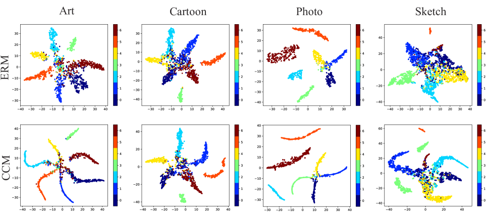
Figure 3: The Visualization results of T-SNE (Van der Maaten and Hinton 2008) on PACS. CCM gives clearer boundaries to the categories and makes features belonging to the same category of images more concentrated in feature space $\mathcal{Z}$. Not only the category mixing area of CCM is smaller, but also the distribution of strip shapes shows that CCM prefers to arrange features with the same category in a manifold manner.

Ablation Study

We further explore the role of each loss of CCM in the overall training process by ablation study. And the results summarized in Table 2. We can find out that applying $\mathcal{L}_{teach}$ alone can significantly improve the performance of domain generalization, and removing $\mathcal{L}_{teach}$ will cause the accuracies of CCM to drop sharply, close to the accuracy of random predictions. It indicates that CCM learns the basic correlations by $\mathcal{L}_{teach}$ and causal effect learning relies on correlations.

Since causal effect learning requires the assistance of contrastive similarity to complete the quantification of causal effects, $L_{learn}$ and $L_{CS}$ need to exist simultaneously to achieve optimal performance. In Table 2, combining $L_{learn}$ and $L_{CS}$ achieves better results on PACS, OfficeHome, and average. We provide the results of ablation experiments for each domain on PACS, OfficeHome, and TerraIncognita in the Appendix.

Visualization

We use T-SNE (Van der Maaten and Hinton 2008) to display the classification results of CCM on PACS visually. Each column represents a domain and each row represents a model. To demonstrate how CCM can distinguish different features in space $\mathcal{Z}$, we feed target domain images in CCM to get their corresponding features and apply T-SNE for dimensionality reduction and visualization. The results are presented in Fig 3. We can find CCM clusters features of images that belong to the same category more closely. Compared with ERM, not only the category boundaries of CCM are more explicit, but also the distributions of features that belong to the same category are more concentrated in the feature space $\mathcal{Z}$. Most of the shapes in the CCM visualization results are stripes, meaning CCM learns more accurate similarity relationships between features of the same category and arranges them by a manifold via contrastive similarity learning.

Conclusion

In this paper, we investigated how to quantify causal effects from images to labels and optimize them. Inspired by the ability of humans to adapt to new environments with prior knowledge, we proposed a novel algorithm called Contrastive Causal Model (CCM), which can transfer unseen images into seen images and quantify the causal effects via the front-door criterion. Through extensive experiments, CCM demonstrates its effectiveness and outperforms current methods. In particular, the prior knowledge of CCM can take many forms, which is the potential to combine with non-image representations to solve multimodal problems.

References

- Arjovsky et al. (2019) Arjovsky, M.; Bottou, L.; Gulrajani, I.; and Lopez-Paz, D. 2019. Invariant risk minimization. arXiv preprint arXiv:1907.02893.
- Balaji, Sankaranarayanan, and Chellappa (2018) Balaji, Y.; Sankaranarayanan, S.; and Chellappa, R. 2018. Metareg: Towards domain generalization using meta-regularization. In Advances in Neural Information Processing Systems (NeurIPS), 998–1008.
- Beery, Van Horn, and Perona (2018) Beery, S.; Van Horn, G.; and Perona, P. 2018. Recognition in terra incognita. In Proceedings of the European conference on computer vision (ECCV), 456–473.
- Blanchard et al. (2017) Blanchard, G.; Deshmukh, A. A.; Dogan, U.; Lee, G.; and Scott, C. 2017. Domain generalization by marginal transfer learning. arXiv preprint arXiv:1711.07910.
- Carlucci et al. (2019) Carlucci, F. M.; D’Innocente, A.; Bucci, S.; Caputo, B.; and Tommasi, T. 2019. Domain Generalization by Solving Jigsaw Puzzles. Proceedings of the IEEE Conference on Computer Vision and Pattern Recognition (CVPR), 2224–2233.
- Chen et al. (2020) Chen, T.; Kornblith, S.; Norouzi, M.; and Hinton, G. E. 2020. A Simple Framework for Contrastive Learning of Visual Representations. In Proceedings of the 37th International Conference on Machine Learning, ICML 2020, 13-18 July 2020, Virtual Event, volume 119 of Proceedings of Machine Learning Research, 1597–1607. PMLR.
- Chen and He (2021) Chen, X.; and He, K. 2021. Exploring simple siamese representation learning. In Proceedings of the IEEE/CVF Conference on Computer Vision and Pattern Recognition, 15750–15758.
- Chen et al. (2021) Chen, Y.; Wang, Y.; Pan, Y.; Yao, T.; Tian, X.; and Mei, T. 2021. A style and semantic memory mechanism for domain generalization. In Proceedings of the IEEE/CVF International Conference on Computer Vision, 9164–9173.
- Christiansen et al. (2021) Christiansen, R.; Pfister, N.; Jakobsen, M. E.; Gnecco, N.; and Peters, J. 2021. A causal framework for distribution generalization. IEEE Transactions on Pattern Analysis and Machine Intelligence.
- Dou et al. (2019) Dou, Q.; de Castro, D. C.; Kamnitsas, K.; and Glocker, B. 2019. Domain generalization via model-agnostic learning of semantic features. In Advances in Neural Information Processing Systems (NeurIPS), 6450–6461.
- Fu et al. (2021) Fu, B.; Cao, Z.; Wang, J.; and Long, M. 2021. Transferable query selection for active domain adaptation. In Proceedings of the IEEE/CVF Conference on Computer Vision and Pattern Recognition, 7272–7281.
- Ganin et al. (2016) Ganin, Y.; Ustinova, E.; Ajakan, H.; Germain, P.; Larochelle, H.; Laviolette, F.; Marchand, M.; and Lempitsky, V. 2016. Domain-adversarial training of neural networks. The journal of machine learning research, 17(1): 2096–2030.
- Gulrajani and Lopez-Paz (2020) Gulrajani, I.; and Lopez-Paz, D. 2020. In search of lost domain generalization. arXiv preprint arXiv:2007.01434.
- He et al. (2020) He, K.; Fan, H.; Wu, Y.; Xie, S.; and Girshick, R. 2020. Momentum contrast for unsupervised visual representation learning. In Proceedings of the IEEE/CVF conference on computer vision and pattern recognition, 9729–9738.
- He et al. (2016) He, K.; Zhang, X.; Ren, S.; and Sun, J. 2016. Deep residual learning for image recognition. In Proceedings of the IEEE conference on computer vision and pattern recognition, 770–778.
- Huang et al. (2020) Huang, Z.; Wang, H.; Xing, E. P.; and Huang, D. 2020. Self-challenging improves cross-domain generalization. In European Conference on Computer Vision, 124–140. Springer.
- Krueger et al. (2021) Krueger, D.; Caballero, E.; Jacobsen, J.-H.; Zhang, A.; Binas, J.; Zhang, D.; Le Priol, R.; and Courville, A. 2021. Out-of-distribution generalization via risk extrapolation (rex). In International Conference on Machine Learning, 5815–5826. PMLR.
- Li et al. (2021a) Li, B.; Shen, Y.; Wang, Y.; Zhu, W.; Reed, C. J.; Zhang, J.; Li, D.; Keutzer, K.; and Zhao, H. 2021a. Invariant information bottleneck for domain generalization. arXiv preprint arXiv:2106.06333.
- Li et al. (2021b) Li, B.; Wang, Y.; Zhang, S.; Li, D.; Keutzer, K.; Darrell, T.; and Zhao, H. 2021b. Learning invariant representations and risks for semi-supervised domain adaptation. In Proceedings of the IEEE/CVF Conference on Computer Vision and Pattern Recognition, 1104–1113.
- Li et al. (2017) Li, D.; Yang, Y.; Song, Y.-Z.; and Hospedales, T. M. 2017. Deeper, broader and artier domain generalization. In Proceedings of the IEEE international conference on computer vision, 5542–5550.
- Li et al. (2018a) Li, D.; Yang, Y.; Song, Y.-Z.; and Hospedales, T. M. 2018a. Learning to generalize: Meta-learning for domain generalization. In Thirty-Second AAAI Conference on Artificial Intelligence.
- Li et al. (2019a) Li, D.; Zhang, J.; Yang, Y.; Liu, C.; Song, Y.-Z.; and Hospedales, T. M. 2019a. Episodic Training for Domain Generalization. Proceedings of the IEEE International Conference on Computer Vision (ICCV), 1446–1455.
- Li et al. (2018b) Li, H.; Pan, S. J.; Wang, S.; and Kot, A. C. 2018b. Domain generalization with adversarial feature learning. In Proceedings of the IEEE conference on computer vision and pattern recognition, 5400–5409.
- Li et al. (2021c) Li, S.; Xie, M.; Gong, K.; Liu, C. H.; Wang, Y.; and Li, W. 2021c. Transferable semantic augmentation for domain adaptation. In Proceedings of the IEEE/CVF Conference on Computer Vision and Pattern Recognition, 11516–11525.
- Li et al. (2021d) Li, S.; Xie, M.; Lv, F.; Liu, C. H.; Liang, J.; Qin, C.; and Li, W. 2021d. Semantic concentration for domain adaptation. In Proceedings of the IEEE/CVF International Conference on Computer Vision, 9102–9111.
- Li et al. (2018c) Li, Y.; Gong, M.; Tian, X.; Liu, T.; and Tao, D. 2018c. Domain Generalization via Conditional Invariant Representations. In McIlraith, S. A.; and Weinberger, K. Q., eds., Proceedings of the Thirty-Second AAAI Conference on Artificial Intelligence, (AAAI-18), the 30th innovative Applications of Artificial Intelligence (IAAI-18), and the 8th AAAI Symposium on Educational Advances in Artificial Intelligence (EAAI-18), New Orleans, Louisiana, USA, February 2-7, 2018, 3579–3587. AAAI Press.
- Li et al. (2018d) Li, Y.; Tian, X.; Gong, M.; Liu, Y.; Liu, T.; Zhang, K.; and Tao, D. 2018d. Deep domain generalization via conditional invariant adversarial networks. In Proceedings of the European Conference on Computer Vision (ECCV), 624–639.
- Li et al. (2019b) Li, Y.; Yang, Y.; Zhou, W.; and Hospedales, T. 2019b. Feature-critic networks for heterogeneous domain generalization. In International Conference on Machine Learning (ICML), 3915–3924. PMLR.
- Liu et al. (2021) Liu, C.; Sun, X.; Wang, J.; Tang, H.; Li, T.; Qin, T.; Chen, W.; and Liu, T.-Y. 2021. Learning causal semantic representation for out-of-distribution prediction. Advances in Neural Information Processing Systems, 34.
- Mahajan, Tople, and Sharma (2021) Mahajan, D.; Tople, S.; and Sharma, A. 2021. Domain generalization using causal matching. In International Conference on Machine Learning, 7313–7324. PMLR.
- Matsuura and Harada (2020) Matsuura, T.; and Harada, T. 2020. Domain Generalization Using a Mixture of Multiple Latent Domains. In Proceedings of the AAAI Conference on Artificial Intelligence (AAAI).
- Nam et al. (2021) Nam, H.; Lee, H.; Park, J.; Yoon, W.; and Yoo, D. 2021. Reducing domain gap by reducing style bias. In Proceedings of the IEEE/CVF Conference on Computer Vision and Pattern Recognition, 8690–8699.
- Rame, Dancette, and Cord (2021) Rame, A.; Dancette, C.; and Cord, M. 2021. Fishr: Invariant gradient variances for out-of-distribution generalization. arXiv preprint arXiv:2109.02934.
- Sagawa et al. (2019) Sagawa, S.; Koh, P. W.; Hashimoto, T. B.; and Liang, P. 2019. Distributionally robust neural networks for group shifts: On the importance of regularization for worst-case generalization. arXiv preprint arXiv:1911.08731.
- Shahtalebi et al. (2021) Shahtalebi, S.; Gagnon-Audet, J.-C.; Laleh, T.; Faramarzi, M.; Ahuja, K.; and Rish, I. 2021. Sand-mask: An enhanced gradient masking strategy for the discovery of invariances in domain generalization. arXiv preprint arXiv:2106.02266.
- Shankar et al. (2018) Shankar, S.; Piratla, V.; Chakrabarti, S.; Chaudhuri, S.; Jyothi, P.; and Sarawagi, S. 2018. Generalizing Across Domains via Cross-Gradient Training. In International Conference on Learning Representations (ICLR).
- Sun and Saenko (2016) Sun, B.; and Saenko, K. 2016. Deep coral: Correlation alignment for deep domain adaptation. In European conference on computer vision, 443–450. Springer.
- Sun et al. (2021) Sun, X.; Wu, B.; Zheng, X.; Liu, C.; Chen, W.; Qin, T.; and Liu, T.-Y. 2021. Recovering Latent Causal Factor for Generalization to Distributional Shifts. Advances in Neural Information Processing Systems, 34.
- Sun et al. (2020) Sun, Y.; Wang, X.; Liu, Z.; Miller, J.; Efros, A.; and Hardt, M. 2020. Test-time training with self-supervision for generalization under distribution shifts. In International conference on machine learning, 9229–9248. PMLR.
- Van der Maaten and Hinton (2008) Van der Maaten, L.; and Hinton, G. 2008. Visualizing data using t-SNE. Journal of machine learning research, 9(11).
- Vapnik (1999) Vapnik, V. 1999. The nature of statistical learning theory. Springer science & business media.
- Venkateswara et al. (2017) Venkateswara, H.; Eusebio, J.; Chakraborty, S.; and Panchanathan, S. 2017. Deep hashing network for unsupervised domain adaptation. In Proceedings of the IEEE conference on computer vision and pattern recognition, 5018–5027.
- Volpi et al. (2018) Volpi, R.; Namkoong, H.; Sener, O.; Duchi, J. C.; Murino, V.; and Savarese, S. 2018. Generalizing to unseen domains via adversarial data augmentation. In Advances in neural information processing systems (NeurIPS), 5334–5344.
- Wald et al. (2021) Wald, Y.; Feder, A.; Greenfeld, D.; and Shalit, U. 2021. On calibration and out-of-domain generalization. Advances in Neural Information Processing Systems, 34.
- Wang and Liu (2021) Wang, F.; and Liu, H. 2021. Understanding the behaviour of contrastive loss. In Proceedings of the IEEE/CVF conference on computer vision and pattern recognition, 2495–2504.
- Wang et al. (2020) Wang, S.; Yu, L.; Li, C.; Fu, C.-W.; and Heng, P. 2020. Learning from Extrinsic and Intrinsic Supervisions for Domain Generalization. In European conference on computer vision (ECCV).
- Yan et al. (2020) Yan, S.; Song, H.; Li, N.; Zou, L.; and Ren, L. 2020. Improve unsupervised domain adaptation with mixup training. arXiv preprint arXiv:2001.00677.
- Yang et al. (2021) Yang, X.; Zhang, H.; Qi, G.; and Cai, J. 2021. Causal attention for vision-language tasks. In Proceedings of the IEEE/CVF Conference on Computer Vision and Pattern Recognition, 9847–9857.
- Yuan et al. (2021) Yuan, J.; Ma, X.; Kuang, K.; Xiong, R.; Gong, M.; and Lin, L. 2021. Learning Domain-Invariant Relationship with Instrumental Variable for Domain Generalization. arXiv preprint arXiv:2110.01438.
- Zhang et al. (2020) Zhang, M.; Marklund, H.; Dhawan, N.; Gupta, A.; Levine, S.; and Finn, C. 2020. Adaptive Risk Minimization: Learning to Adapt to Domain Shift. arXiv preprint arXiv:2007.02931.
- Zhang et al. (2021) Zhang, X.; Cui, P.; Xu, R.; Zhou, L.; He, Y.; and Shen, Z. 2021. Deep stable learning for out-of-distribution generalization. In Proceedings of the IEEE/CVF Conference on Computer Vision and Pattern Recognition, 5372–5382.
- Zhao et al. (2020) Zhao, S.; Gong, M.; Liu, T.; Fu, H.; and Tao, D. 2020. Domain Generalization via Entropy Regularization. In Advances in Neural Information Processing Systems (NeurIPS).
- Zhou et al. (2020a) Zhou, K.; Yang, Y.; Hospedales, T.; and Xiang, T. 2020a. Learning to generate novel domains for domain generalization. In European Conference on Computer Vision (ECCV), 561–578.
- Zhou et al. (2020b) Zhou, K.; Yang, Y.; Hospedales, T. M.; and Xiang, T. 2020b. Deep Domain-Adversarial Image Generation for Domain Generalisation. In The Thirty-Fourth AAAI Conference on Artificial Intelligence, AAAI 2020, The Thirty-Second Innovative Applications of Artificial Intelligence Conference, IAAI 2020, The Tenth AAAI Symposium on Educational Advances in Artificial Intelligence, EAAI 2020, New York, NY, USA, February 7-12, 2020, 13025–13032. AAAI Press.
- Zhou et al. (2021) Zhou, K.; Yang, Y.; Qiao, Y.; and Xiang, T. 2021. Domain Generalization with Mixstyle. In International Conference on Learning Representations (ICLR).