Decision Making under Cumulative Prospect Theory: An Alternating Direction Method of Multipliers

Abstract

This paper proposes a novel numerical method for solving the problem of decision making under cumulative prospect theory (CPT), where the goal is to maximize utility subject to practical constraints, assuming only finite realizations of the associated distribution are available. Existing methods for CPT optimization rely on particular assumptions that may not hold in practice. To overcome this limitation, we present the first numerical method with a theoretical guarantee for solving CPT optimization using an alternating direction method of multipliers (ADMM). One of its subproblems involves optimization with the CPT utility subject to a chain constraint, which presents a significant challenge. To address this, we develop two methods for solving this subproblem. The first method uses dynamic programming, while the second method is a modified version of the pooling-adjacent-violators algorithm that incorporates the CPT utility function. Moreover, we prove the theoretical convergence of our proposed ADMM method and the two subproblem-solving methods. Finally, we conduct numerical experiments to validate our proposed approach and demonstrate how CPT’s parameters influence investor behavior using real-world data.

1 Introduction

Cumulative Prospect Theory (CPT, Kahneman and Tversky, 1979, Tversky and Kahneman, 1992) is a popular model for descriptive decisions under risk and uncertainty in behavioral economics. It describes four behaviour characteristics of the decision makers: (i) they assess the random outcomes as gains or losses with respect to a reference point, (ii) they are loss-averse, which means that they suffer more from losing than they enjoy from winning by the same amount, (iii) they are risk-averse for gains and risk-seeking for losses, and (iv) they assign more subjective weights to the outcomes with low objective probability. The CPT model is widely applied in various fields, such as portfolio selection (He and Zhou, 2011), operations management (Nagarajan and Shechter, 2014), supply chain management (Liu et al., 2013), transportation management (Li et al., 2015), etc.

The CPT model induces an S-shaped utility function, which is nonconvex and nonsmooth at the reference point, and inverse S-shaped probability weighting functions. These features make the decision making problems under CPT challenging to solve. A majority of the literature deals with these problems by imposing specific assumptions such as thee normal distribution assumption (Barberis and Huang, 2008, Liu et al., 2013), the elliptical distribution assumption (Shi et al., 2015a ), the binomial tree assumption (Barberis and Xiong, 2009), the one dimensional random source assumption (Bernard and Ghossoub, 2010, He and Zhou, 2011, Nagarajan and Shechter, 2014, Shi et al., 2015b ), the complete market assumption (Jin and Zhou, 2008, van Bilsen and Laeven, 2020) and the piece-wise linear utility function assumption (De Giorgi and Legg, 2012, Shi et al., 2015a ). On the other hand, there are only limited numerical algorithms for solving the CPT models, such as heuristics based algorithms (Levy and Levy, 2004), and generic nonlinear optimizers (Srivastava et al., 2022). Very recently, Luxenberg et al., (2022) propose three numerical optimization methods for solving CPT optimization. However, their methods only apply to an approximation of the original CPT optimization problem by enforcing monotonicity on weights (see Section 2.2 in Luxenberg et al., 2022 for the discussion). To the best of our knowledge, there is no existing method that can solve the CPT optimization problem with a general setting.

We aim to solve the CPT optimization problem with a general setting by the alternating direction method of multipliers (ADMM). ADMM is a popular optimization method for problems that have a certain separable structure in objective functions (Glowinski and Marrocco, 1977). Its main advantage is that using the separable structure, the subproblems in ADMM are easy to solve. ADMM finds numerous applications in real world such as statistical learning (Scheinberg et al., 2010), portfolio optimization (Cui et al., 2018) and signal processing (Combettes and Pesquet, 2007). For more details on the ADMM algorithm, we refer to the survey paper Boyd et al., (2011).

In this paper, we consider the following decision making model under CPT,

$$\min_{{\mathbf{x}}} \quad\int U(z)d\omega(1-F_{Z}(z))\quad {\rm s.t.}~{}Z={\mathbf{r}}^{T}{\mathbf{x}},\quad{\mathbf{x}}\in\mathcal{X}.$$ (1)

Here, $U:\mathbb{R}\to\mathbb{R}$ is the utility function, $\omega:[0,1]\to[0,1]$ is the probability weighting function, ${\mathbf{r}}$ is a $d$-dimensional random vector, ^T denotes the transpose operator, $F_{Z}(z)$ denotes the cumulative distribution function of random variable $Z$, and $\mathcal{X}$ is the feasible set for decision variable ${\mathbf{x}}$. In real-world applications, it is difficult to know the true distribution of the random variable ${\mathbf{r}}$. Instead, we can often access finite realizations of the distribution via either historical data or sample points generated by simulation. Given $N$ realizations of ${\mathbf{r}}$, the problem becomes

$$\min_{{\mathbf{x}}} \quad-\sum_{i=1}^{N}c_{i}U((R{\mathbf{x}})_{[i]})\quad {\rm s.t.}~{}{\mathbf{x}}\in\mathcal{X},$$ (2)

where $R\in{\mathbb{R}}^{N\times d}$ is the matrix formed by $N$ scenarios of ${\mathbf{r}}$, $(R{\mathbf{x}})_{[i]}$ is the $i$th smallest component of $R{\mathbf{x}}$, and $c_{i}$ is the rank-dependent weight on $(R{\mathbf{x}})_{[i]}$ with expression $c_{i}=\omega(\frac{N-i+1}{N})-\omega(\frac{N-i}{N}),$ which depends on the probability weighting function $\omega$ (defined in Section 2). The difficulty of this problem stems from the possible nonconvexity and nonsmoothness of $U$, the nonconvexity induced by $\omega$, and the rank of $(R{\mathbf{x}})_{[i]}$.

The main contribution of this paper is to propose an ADMM algorithm. We first reformulate (2) by introducing an auxiliary variable ${\mathbf{y}}=R{\mathbf{x}}$. Utilizing the structure of the new reformulation with the auxiliary variable, we then develop an ADMM as a solution method. We also demonstrate the global convergence of the ADMM method. The ${\mathbf{x}}$-subproblem of the ADMM, which is a convex quadratic program when ${\mathcal{X}}$ is a polyhedron, is easy to solve. However, the ${\mathbf{y}}$-subproblem has a nonconvex finite sum objective with rank-dependent weights, which makes it extremely different to solve. To address this challenge, we develop a dynamic programming (DP) method to solve this subproblem. We demonstrate that the DP method can find the global optimal solution. Despite the solidness in theory, the DP method may be slow in practice if there are a large number of historical scenarios of the randomness. To improve practical efficiency, we further propose a variant of the celebrated pooling-adjacent-violators (PAV) algorithm to solve this subproblem, which can be seen as an extension of the PAV algorithm for convex programming (Ayer et al., 1955, Brunk et al., 1972, Best and Chakravarti, 1990, Ahuja and Orlin, 2001). We further prove that the PAV algorithm converges to a stationary point of a reformulation of the subproblem. Our numerical study shows that the proposed ADMM outperforms the general solver fmincon in MATLAB, and the ADMM with PAV as its subproblem performs better than that equipped with the DP. We also conduct an empirical portfolio selection study based on 48 industry indices of the US market and investigate the impacts of CPT’s parameters on the optimal portfolio.

The remaining of this paper is organized as follows. In Section 2, we specify the expression of the decision making problem under CPT. Then in Section 3, we propose the ADMM framework and derive its convergence analysis. In Section 4, we propose two methods, the DP and the PAV methods, to solve the ${\mathbf{y}}$-subproblem in the ADMM. In Section 5, we conduct numerical experiments to show the effectiveness of the proposed method. We conclude our paper in Section 6.

2 The decision making problem under CPT

In the decision-making problem under CPT (1), the utility function and probability weighting function are key components that describe the decision maker’s preferences. According to Tversky and Kahneman Tversky and Kahneman, (1992), the decision maker has an S-shaped utility function of the form

$$U(z)=\left\{\begin{aligned} &-\mu(B-z)^{\alpha},&z\leq B,\\ &(z-B)^{\alpha},&z>B,\end{aligned}\right.$$ (3)

where $B$ is the reference point that defines gains and losses, $\mu>1$ is the loss aversion parameter, and $\alpha$ is the degree of relative risk aversion (or risk seeking) for gains (or losses). Furthermore, the decision makers evaluate the probability for gains and losses through the following probability weighting function,

$$\omega(1-F_{Z}(z))=\left\{\begin{aligned} &\frac{F_{Z}(z)^{\gamma}}{((1-F_{Z}(z))^{\gamma}+F_{Z}(z)^{\gamma})^{1/\gamma}},&z\leq B,\\[5.69054pt] &\frac{(1-F_{Z}(z))^{\delta}}{((1-F_{Z}(z))^{\delta}+F_{Z}(z)^{\delta})^{1/\delta}},&z>B,\end{aligned}\right.$$ (4)

where $\gamma$ is the probability distortion parameter for losses, and $\delta$ is the probability distortion parameter for gains. When the random vector ${\mathbf{r}}$ has $N$ realizations, which are collected in an $N\times d$ matrix $R$, the decision making model under CPT becomes the optimization problem (2).

We point out that the CPT optimization problem (2) can represent a portfolio optimization problem whose objective is to maximize the CPT utility, where $R$ represents the matrix formed by $N$ historical return of $d$ assets, $R{\mathbf{x}}$ represents the historical return of the portfolio ${\mathbf{x}}$, and $c_{i}$ is the weight associated with the $i$th order statistics of historical return of the portfolio. When we choose a strictly concave utility and a single inverse S-shaped probability weighting function, the portfolio optimization model under CPT becomes the rank dependent utility maxization problem (RDU, Quiggin, 2012). Furthermore, when we choose the identity map $U(y)=y$ and different weights $c_{i}$, problem (2) includes many risk management problems. When $c_{i}=1$ for $i=\lceil\alpha N\rceil$ and $c_{i}=0$ otherwise, the objective function reduces to Value at Risk at confidence level $\alpha\in(0.5,1)$ (VaR, Duffie and Pan, 1997,Cui et al., 2018), where $\lceil\alpha N\rceil$ is the smallest integer that is larger than or equal to $\alpha N$. When $c_{i}=\frac{1}{N-\lceil\alpha N\rceil+1}$ for $i\geq\lceil\alpha N\rceil$ and $c_{i}=0$ otherwise, the objective function reduces to Conditional Value at Risk at confidence level $\alpha$ (CVaR, Rockafellar et al., 2000). When $\sum_{i=1}^{N}c_{i}=1$ and $0\leq c_{1}\leq\dots\leq c_{N}\leq 1$, then the objective function is the spectral risk measure (SRM, Acerbi, 2002). When $\sum_{i=1}^{N}c_{i}=1$ and $0\leq c_{i}$, then the objective function is the distortion risk measure (DRM, Dhaene et al., 2006). As the rank-depenent weights $c_{i}$ in VaR and distortion risk measure are not decreasing functions of $i$, the corresponding risk management problems are not convex and hard to solve.

To make our research applicable to a more general setting, we consider the decision making problem under CPT (2), which does not specify the concrete form of the utility function, and only requires the utility function satisfying the following assumption.

Assumption 1

Assume the function $U:{\mathbb{R}}\to{\mathbb{R}}$ in problem (2) satisfies the following properties.

1. $U$ is a strictly increasing, continuous function in ${\mathbb{R}}$.

2. $U$ is a third order continuously differentiable function in either $(-\infty,B)$ or $(B,\infty)$.

3. When $z\in(-\infty,B)$, we have $U^{\prime\prime}(z)>0$. When $z\in(B,\infty)$, we have $U^{\prime\prime}(z)<0$.

4. When $z\in(-\infty,B)$, we have $U{{}^{\prime\prime\prime}}(z)>0$.

5. If $U{{}^{\prime}}(B^{-})=\infty$, then $U{{}^{\prime}}(B^{+})=\infty$, and vice versa, where $U{{}^{\prime}}(\theta^{+})=\lim_{y\rightarrow\theta^{+}}U{{}^{\prime}}(y)$, and $U{{}^{\prime}}(\theta^{-})=\lim_{y\rightarrow\theta^{-}}U{{}^{\prime}}(y)$.

These properties are the generalizations of the utility function proposed in Tversky and Kahneman, (1992).

3 The ADMM Algorithm

In this section, we propose an alternating direction method of multipliers (ADMM) to solve problem (2). Among all the utilities used in the literature, the CPT utility poses the most difficulty for optimization. Therefore, we focus on the CPT optimization in this section and give a remark on other risk preferences that our method can handle at the end of this section. Note that the main challenge of optimizing (2) stems from the utility function, which is nonsmooth and nonconvex. At first glance, the nonsmoothness arises from the order statistics of $R{\mathbf{x}}$, which are finite realizations of terminal wealth, and the nonconvexity arises from the S-shaped utility. However, we point out that a more subtle issue is that the probability distortion (4) and rank of realizations of terminal wealth introduce additional nonconvexity and nonsmoothness that depend on both the values of terminal wealth realizations and the reference point $B$.

To address the difficulty in the utility function, we introduce an auxiliary variable ${\mathbf{y}}\in{\mathbb{R}}^{N}$ to represent terminal wealth realizations. That is, we reformulate problem (2) as

$$\min_{{\mathbf{x}},{\mathbf{y}}} \quad-\sum_{i=1}^{N}c_{i}U(y_{[i]})+I_{\mathcal{X}}({\mathbf{x}}) \quad{\rm s.t.}~{}{\mathbf{y}}=R{\mathbf{x}},$$ (5)

where $I_{\mathcal{X}}({\mathbf{x}})=0$ if ${\mathbf{x}}\in\mathcal{X}$ and $\infty$ otherwise is the indicator function of set $\mathcal{X}$. The augmented Lagrangian function of problem (5) is

$$L_{\sigma}({\mathbf{x}},{\mathbf{y}};{\boldsymbol{\lambda}})=-\sum_{i=1}^{N}c_{i}U(y_{[i]})+I_{\mathcal{X}}({\mathbf{x}})+\langle{\boldsymbol{\lambda}},{\mathbf{y}}-R{\mathbf{x}}\rangle+\frac{\sigma}{2}\left\|{\mathbf{y}}-R{\mathbf{x}}\right\|_{2}^{2},$$

where ${\boldsymbol{\lambda}}$ is the Lagrange multiplier and $\sigma>0$ is the quadratic penalty parameter. Note that it is difficult to simultaneously optimize ${\mathbf{x}}$ and ${\mathbf{y}}$ in the augmented Lagrangian function. This motivates us to adopt the ADMM framework that is widely used to handle a separable objective function. The update of ADMM is as follows

$${\mathbf{x}}^{k+1} ={\mathop{\text{argmin}}}_{{\mathbf{x}}\in\mathcal{X}}~{}L_{\sigma}({\mathbf{x}},{\mathbf{y}}^{k};{\boldsymbol{\lambda}}^{k}),$$ (6a)

$${\mathbf{y}}^{k+1} ={\mathop{\text{argmin}}}_{{\mathbf{y}}}~{}L_{\sigma}({\mathbf{x}}^{k+1},{\mathbf{y}};{\boldsymbol{\lambda}}^{k}),$$ (6b)

$${\boldsymbol{\lambda}}^{k+1} ={\boldsymbol{\lambda}}^{k}+\sigma({\mathbf{y}}^{k+1}-R{\mathbf{x}}^{k+1}).$$ (6c)

We summarise our ADMM framework in Algorithm 1.

The ${\mathbf{x}}$-subproblem (6a) is equivalent to a quadratic program when $\mathcal{X}$ is a polyhedron,

$$\min_{{\mathbf{x}}\in{\mathcal{X}}} \quad\frac{\sigma}{2}\left\|{\mathbf{y}}^{k}-R{\mathbf{x}}+\frac{{\boldsymbol{\lambda}}^{k}}{\sigma}\right\|_{2}^{2},$$

which can be easily solved by off-the-shelf solvers.

Algorithm 1 ADMM for CPT optimization problem (2)

1:$R,~{}\sigma,~{}\epsilon_{1},~{}\epsilon_{2},~{}{\mathbf{y}}^{0},~{}{\boldsymbol{\lambda}}^{0}$, and $k=0$

2:repeat

3:    Solve (6a) to obtain ${\mathbf{x}}^{k+1}$

4:    Solve (6b) to obtain ${\mathbf{y}}^{k+1}$ either exactly or approximately

5:    Update $\boldsymbol{\lambda^{k+1}}=\boldsymbol{\lambda^{k}}+\sigma({\mathbf{y}}^{k+1}-R{\mathbf{x}}^{k+1})$

6:    $k=k+1$

7:until $\|{\mathbf{y}}^{k}-R{\mathbf{x}}^{k}\|\leq\epsilon_{1}$ and $\|{\mathbf{y}}^{k}-{\mathbf{y}}^{k-1}\|\leq\epsilon_{2}$

The main difficulty lies in solving the ${\mathbf{y}}$-subproblem (6b), which is a nonconvex and nonsmooth optimization problem. Fortunately, by exploiting the structure of the ${\mathbf{y}}$-subproblem, we propose two efficient algorithms, whose details are given in Section 4. At the $k$th iteration, the ${\mathbf{y}}$-subproblem is to minimize the following function

$$\Phi({\mathbf{y}})=-\sum_{i=1}^{N}c_{i}U(y_{[i]})+\frac{\sigma}{2}\left\|{\mathbf{y}}-R{\mathbf{x}}^{k+1}+\frac{{\boldsymbol{\lambda}}^{k}}{\sigma}\right\|^{2}.$$

Before presenting our convergence analysis of the proposed ADMM algorithm, let us first introduce some results from nonsmooth analysis. Let $\Omega({\mathbf{y}})$ denote the first component of $\Phi({\mathbf{y}})$, i.e., $\Omega({\mathbf{y}})=-\sum_{i=1}^{N}c_{i}U(y_{[i]}).$ We show that both $\Phi({\mathbf{y}})$ and $\Omega({\mathbf{y}})$ are locally Lipschitz functions under mild conditions so that the stationary point can be characterized by the Clarke generalized gradient (Clarke, 1990). Recall that $U’(B)<\infty$ represent that both $U’(B^{-})<\infty$ and $U’(B^{+})<\infty$.

Lemma 1

Under 1, the functions $\Phi({\mathbf{y}})$ and $\Omega({\mathbf{y}})$ are both locally Lipschitz continuous in some neighbourhood of any given $\bar{\mathbf{y}}$ satisfying $U’(\bar{y}_{i})<\infty$.

The proofs in this paper are all deferred to Appendix A. We remark that $\Omega(y)$ is non-Lipschitz at $y_{i}=B$ for the S-shape power utility (3). As we have shown that $\Omega({\mathbf{y}})$ is locally Lipschitz for every ${\mathbf{y}}$ as long as $U^{\prime}(y_{i})<\infty~{}\forall i$, the Clarke generalized gradient of $\Omega({\mathbf{y}})$, denoted by $\partial\Omega({\mathbf{y}})$, exists if $U^{\prime}(y_{i})<\infty~{}\forall i$ (Clarke, 1990). Let $\chi({\mathbf{x}})=\Omega(R{\mathbf{x}})$. By the chain rule, we have

$$\partial\chi({\mathbf{x}})\subset R^{T}\partial\Omega(R{\mathbf{x}}).$$

Denote by $N_{\mathcal{X}}(\bar{\mathbf{x}})$ the normal cone of $\mathcal{X}$ at $\bar{\mathbf{x}}\in{\mathcal{X}}$, i.e., $N_{\mathcal{X}}(\bar{\mathbf{x}})=\{{\mathbf{z}}\in\mathbb{R}^{d}\mid\langle{\mathbf{z}},{\mathbf{x}}-\bar{\mathbf{x}}\rangle\leq 0,~{}\forall{\mathbf{x}}\in\mathcal{X}\}.$ It is well known that $\partial I_{\mathcal{X}}({\mathbf{x}})=N_{\mathcal{X}}({\mathbf{x}})$; see, e.g., (Beck, 2017, Example 3.5). We then have

$$\partial\left(\chi({\mathbf{x}})+I_{\mathcal{X}}({\mathbf{x}})\right)\subset\partial\chi({\mathbf{x}})+\partial I_{\mathcal{X}}({\mathbf{x}})=\partial\chi({\mathbf{x}})+N_{\mathcal{X}}({\mathbf{x}}),$$

where the first inclusion is due to Corollary 1 of (Clarke, 1990, Theorem 2.9.8). Suppose ${\mathbf{x}}^{*}$ is a local minimizer of (6b). Then from (Clarke, 1990, Proposition 2.3.2) we have ${\mathbf{0}}\in\partial\left(\chi({\mathbf{x}}^{*})+I_{\mathcal{X}}({\mathbf{x}}^{*})\right).$ The above facts imply the following necessary optimality condition

$${\mathbf{0}}\in R^{T}\partial\Omega(R{\mathbf{x}}^{*})+N_{\mathcal{X}}({\mathbf{x}}^{*}).$$ (7)

Let ${\mathbf{y}}$ be such that $\Omega$ is locally Lipschitz near ${\mathbf{y}}$. Due to (Clarke, 1990, Theorem 2.5.1), we have

$$\partial\Omega({\mathbf{y}})={\rm conv}\left(\{\lim_{i\to\infty}\nabla\Omega({\mathbf{y}}^{i}):~{}{\mathbf{y}}^{i}\to{\mathbf{y}},~{}{\mathbf{y}}^{i}\notin S,~{}\Omega\text{ is differentiable at }{\mathbf{y}}^{i}\}\right).$$

where ${\rm conv}(A)$ denotes the convex hull of set $A$. In fact, using the structure of $\Omega({\mathbf{y}})$, we can characterize the expression of $\partial\Omega({\mathbf{y}})$ explicitly by considering the coordinates that are equivalent. Let $\{i_{1},i_{2},\ldots,i_{s^{k}}\}$ be a permutation of $\{1,\ldots,N\}$ and ${\mathbf{y}}$ be such that

$$y_{i_{s^{1}+1}}=\cdots=y_{i_{s^{2}}}<\cdots<y_{i_{s}^{k-1}+1}=\cdots=y_{i_{s^{k}}}.$$

where we use the convention $s^{1}=0$ and $s^{k}=N$. Note that except the points that are equivalent to $B$, the only non-differentiable points are those where at least two coordinates have the same value. We then have

$$\begin{array}[]{ll}\partial\Omega({\mathbf{y}})={\rm conv}\left(\left\{{\mathbf{v}}:\right.\right.{}&v_{i_{j}}\in-c_{i_{j}}\partial U(y_{i_{j}}),~{}j=s^{t}+1,\ldots,s^{t+1},~{}t=1,\ldots,k,\\ &\left.\left.\{i_{1},i_{2},\ldots,i_{s^{k}}\}\text{ is a permutation of }\{1,\ldots,N\}\right\}\right).\end{array}$$ (8)

We remark that $\partial U(y_{i_{j}})$ is always a singleton when $y_{i_{j}}\neq B$, and $\partial U(B)={\rm conv}\{U(B^{-}),U(B^{+})\}$ is an interval. Let us illustrate this using a simple example. If ${\mathbf{y}}=(y_{1},y_{2},y_{3})$ with $y_{2}=y_{3}<y_{1}$, then we must have either $y_{[1]}=y_{2},~{}y_{[2]}=y_{3},~{}y_{[3]}=y_{1}$ or $y_{[1]}=y_{3},~{}y_{[2]}=y_{2},~{}y_{[3]}=y_{1}$, and thus

$$\partial\Omega({\mathbf{y}})={\rm conv}\left(\{(-c_{3}U^{\prime}(y_{1}),-c_{1}U^{\prime}(y_{2}),-c_{2}U^{\prime}(y_{3}))^{T},(-c_{3}U^{\prime}(y_{1}),-c_{2}U^{\prime}(y_{2}),-c_{1}U^{\prime}(y_{3}))^{T}\}\right).$$

We then directly have from (8) the following lemma that is useful in our convergence analysis.

Lemma 2 (Outer semicontinuity)

Let ${\mathbf{y}}$ be such that $\Omega$ is locally Lipschitz near ${\mathbf{y}}$. Then for any sequences $\{{\mathbf{v}}^{k}\}$ and $\{{\mathbf{y}}^{k}\}$ such that ${\mathbf{v}}^{k}\to{\mathbf{v}}^{*}$, ${\mathbf{y}}^{k}\to{\mathbf{y}}^{*}$ and ${\mathbf{v}}^{k}\in\partial\Omega({\mathbf{y}}^{k})$, we have ${\mathbf{v}}^{*}\in\partial\Omega({\mathbf{y}}^{*})$.

As the main theoretical result in this section, we will show that the proposed ADMM algorithm converges to a point satisfying the necessary optimality condition (7) under mild conditions. To this end, let us first make an assumption on the sequence of Lagrange multiplier.

Assumption 2

The sequence $\{{\boldsymbol{\lambda}}^{k}\}$ is bounded and satisfies the following condition

$$\sum_{k=1}^{\infty}\|{\boldsymbol{\lambda}}^{k+1}-{\boldsymbol{\lambda}}^{k}\|^{2}<\infty.$$

We remark that 2 is widely used in the ADMM literature; see, e.g., Xu et al., (2012) and Bai et al., (2021). A stronger version of this assumption is used in Shen et al., (2014).

We also impose the following assumption on the solutions of the ${\mathbf{x}}$- and ${\mathbf{y}}$-subproblem.

Assumption 3

The ${\mathbf{x}}$-subproblem is globally solved. The ${\mathbf{y}}$-subproblem is solved such that

$$L_{\sigma}({\mathbf{x}}^{k+1},{\mathbf{y}}^{k};{\boldsymbol{\lambda}}^{k})-L_{\sigma}({\mathbf{x}}^{k+1},{\mathbf{y}}^{k+1};{\boldsymbol{\lambda}}^{k})\geq 0,\quad\text{and}$$ (9)

$${\mathbf{0}}\in\partial\Omega({\mathbf{y}}^{k+1})+\sigma\left({\mathbf{y}}^{k+1}-R{\mathbf{x}}^{k+1}+\frac{{\boldsymbol{\lambda}}^{k}}{\sigma}\right).$$ (10)

We remark that the above assumption is quite mild. Indeed, the ${\mathbf{x}}$-subproblem is a convex program if $\mathcal{X}$ is a convex set, which can be solved globally by many methods such as interior point methods (Nocedal and Wright, 1999). Meanwhile, the ${\mathbf{y}}$-subproblem is solved to a stationary point ${\mathbf{y}}^{k+1}$ that has an objective value not exceeding that of the initial point ${\mathbf{y}}^{k}$. We will propose a subproblem solver that can return a solution satisfying both (9) and (10) in Section 4.

Now we are ready to present the main convergence result for the ADMM algorithm.

Theorem 1

Suppose that $R^{T}R$ is positive definite, ${\mathcal{X}}$ is a convex and closed set, $\epsilon_{1}=\epsilon_{2}=0$, and Assumptions 2 and 3 hold. Let $\{({\mathbf{x}}^{k},{\mathbf{y}}^{k})\}$ be a sequence generated by the ADMM algorithm. Then any accumulation point of the sequence $\{({\mathbf{x}}^{k},{\mathbf{y}}^{k})\}$, denoted by $({\mathbf{x}}^{*},{\mathbf{y}}^{*})$, satisfies the following condition

$${\mathbf{0}}\in R^{T}\partial\Omega({\mathbf{y}}^{*})+N_{\mathcal{X}}({\mathbf{x}}^{*}),\quad{\mathbf{y}}^{*}=R{\mathbf{x}}^{*}.$$

Hence ${\mathbf{x}}^{*}$ is a stationary point of (2) in the sense that (7) holds.

We remark that the assumption on $R^{T}R$ is mild as $R^{T}R$ is indeed the estimated covariance matrix of assets. It is reasonable that a covariance matrix is positive definite when $N>d$, i.e., the number of realizations exceeds the number of assets. If we relax this assumption, we can add a proximal term in the ${\mathbf{x}}$-subproblem, which modifies our algorithm to a proximal ADMM algorithm like Bai et al., (2021), and obtain a similar convergence result. For simplicity, we omit details for this case. The assumption that ${\mathcal{X}}$ is a convex and closed set is widely used in practice, e.g., in many portfolio optimization applications, the weight has a box constraint or a simplex constraint (Cui et al., 2018).

As a final remark, we point out that the decision making problem (2) becomes easier to solve when $U$ is a strictly concave function or an identity function. This covers the cases of the RDU, VaR, CVaR, SRM and DRM. Comparing to RDU, CVaR, SRM problems, VaR and DRM problem are much harder. However, our ADMM framework can handle these problems as well. Indeed, the ${\mathbf{x}}$-subproblems are still quadratic programs and can be solved by off-the-shelf solvers. The ${\mathbf{y}}$-subproblems for above problems can be shown to be equivalent to convex separable problems with chain constraints and thus can be solved by either off-the-shelf solvers or specific algorithms for convex optimization with chain constraints. For further details, please refer to Remark 1 in the next section.

4 Solving the ${\mathbf{y}}$-Subproblem in the ADMM

In this section, we propose two methods to solve the ${\mathbf{y}}$-subproblem (6b). Before presenting our methods, we first introduce a reformulation for the ${\mathbf{y}}$-subproblem. Let ${\mathbf{w}}^{k+1}=R{\mathbf{x}}^{k+1}-{{\boldsymbol{\lambda}}^{k}}/{\sigma}$. For simplicity, we omit the superscript in ${\mathbf{w}}^{k+1}$ in the following of this section. Let $\{l_{1},l_{2},\dots,l_{N}\}$ be a permutation of $\{1,\ldots,N\}$ such that $w_{l_{1}}\leq w_{l_{2}}\leq\dots\leq w_{l_{N}}.$ As $c_{i}U(y_{[i]})$ is independent on any permutation of ${\mathbf{y}}$, the ${\mathbf{y}}$-subproblem (6b) is equivalent to

$$\min_{{\mathbf{y}}}\quad\sum_{i=1}^{N}-c_{i}U(y_{l_{i}})+\frac{\sigma}{2}(y_{l_{i}}-w_{l_{i}})^{2}\quad\text{s.t.}\quad y_{l_{1}}\leq y_{l_{2}}\leq\dots\leq y_{l_{N}}.$$ (11)

The constraint $y_{l_{1}}\leq y_{l_{2}}\leq\dots\leq y_{l_{N}}$ is known as the simple chain constraint (Best et al., 2000). Such a constraint first occurred in isotonic regression (Ayer et al., 1955) and has been widely studied in the literature (Brunk et al., 1972, Strömberg, 1991). We remark that a similar reformulation idea was previously used in (Cui et al., 2018, Lemma 3).

Remark 1

When the function $U$ is a smooth and strictly concave function, or the identity function, which covers the cases of RDU, VaR, CVaR, SRM, and DRM, problem (11) becomes a convex optimization problem with a separable objective function over the chain constraint, which can be solved by a general convex solver. We can further utilize the celebrated pooling-adjacent-violators (PAV) method (e.g., Best et al., (2000)) or the dynamic programming (DP) method proposed by Yu et al., (2022), which takes advantage of the structure of equation (11), to obtain much faster speed in both theory and practice. Therefore, we focus on the CPT utility function whose subproblem in equation (11) is currently unsolvable by existing methods.

Without loss of generality, in this section we assume $w_{1}\leq w_{2}\leq\dots\leq w_{N}$ for further simplicity of notations. Thus problem (11) is equivalent to the following isotonic program

$$\min_{{\mathbf{y}}}\quad\sum_{i=1}^{N}-c_{i}U(y_{i})+\frac{\sigma}{2}(y_{i}-w_{i})^{2}\quad\text{s.t.}\quad y_{1}\leq y_{2}\leq\dots\leq y_{N}.$$ (12)

Let $f_{i}(y_{i})=-c_{i}U(y_{i})+\frac{\sigma}{2}(y_{i}-w_{i})^{2}$. That is, $f_{i}(y_{i})=\left\{\begin{aligned} -a_{i}U(y_{i})+\frac{\sigma}{2}(y_{i}-w_{i})^{2},\quad y_{i}\leq B,\\ -b_{i}U(y_{i})+\frac{\sigma}{2}(y_{i}-w_{i})^{2},\quad y_{i}>B.\end{aligned}\right.$ Note that according to $c_{i}$ in (4), we have $a_{i}>0$ and $b_{i}>0$. Then problem (12) can be rewritten as

$$\min\quad\sum_{i=1}^{N}f_{i}(y_{i})\quad\text{s.t.}\quad y_{1}\leq y_{2}\leq\dots\leq y_{N}.$$ (13)

We will utilize the structure of $f_{i}$ to design our algorithm.

To this end, we first consider the property of the following function

$$\zeta(y)=\left\{\begin{aligned} &-aU(y)+\frac{\sigma}{2}(y-w)^{2},&y\leq B,\\ &-bU(y)+\frac{\sigma}{2}(y-w)^{2},&y>B,\end{aligned}\right.$$ (14)

where $a,b\geq 0,\sigma>0$. Note that $f_{i}$ is exactly in the form of $\zeta$. It is obvious that $\zeta(y)$ is characterized by parameters $a,b,w,\sigma$, and function $U$. We will sometimes write it in the form $\zeta_{a,b,w,\sigma,U}(y)$ to emphasize the role of $a,b,w,\sigma$, and $U$. The first order and second order derivatives of $\zeta(y)$ are given by

$$\zeta{{}^{\prime}}(y)=\left\{\begin{aligned} &-aU{{}^{\prime}}(y)+\sigma(y-w),&y\leq B,\\ &-bU{{}^{\prime}}(y)+\sigma(y-w),&y>B,\end{aligned}\right.\quad\text{ and }\quad\zeta{{}^{\prime\prime}}(y)=\left\{\begin{aligned} &-aU{{}^{\prime\prime}}(y)+\sigma,&y\leq B,\\ &-bU{{}^{\prime\prime}}(y)+\sigma,&y>B.\end{aligned}\right.$$ (15)

We next introduces properties of $\zeta$ that will be frequently used in the paper.

Fact 1

Assume $a>0,~{}b>0,$ and $\sigma>0$.

We first show that $\zeta(y)$ has at most one local minimizer and no local maximizer in interval $(B,\infty)$. Recall that $U(y)$ satisfies the properties in 1. The function $\zeta(y)$ is strongly convex in $(B,\infty)$ due to $U{{}^{\prime\prime}}(y)<0,~{}b>0$ and $\sigma>0$, and $\zeta{{}^{\prime}}(y)$ is strictly increasing in $(B,\infty)$. We have two cases depends on the value of $\zeta{{}^{\prime}}(B^{+}).$

1. If $\zeta{{}^{\prime}}(B^{+})\geq 0$, then $\zeta{{}^{\prime}}(y)>\zeta{{}^{\prime}}(B^{+})\geq 0$ and thus $\zeta(y)$ is strictly increasing in $(B,\infty)$.

2. If $\zeta{{}^{\prime}}(B^{+})<0$, we have

   $$\zeta{{}^{\prime}}(u)\geq-bU{{}^{\prime}}(B+1)+\sigma(u-w)\geq-bU{{}^{\prime}}(B+1)+\sigma\frac{bU{{}^{\prime}}(B+1)}{\sigma}=0,$$

   where $u=\max\left(B+1,w+\frac{bU{{}^{\prime}}(B+1)}{\sigma}\right)$, and the first inequality follows from that $b>0$ and $U{{}^{\prime\prime}}(y)<0$. As $\zeta{{}^{\prime}}(B^{+})<0$ and $\zeta{{}^{\prime}}(u)\geq 0$, there exits a unique $\xi\in(B,u]$ such that $\zeta{{}^{\prime}}(\xi)=0$. This, together with the fact that $\zeta^{\prime}(y)$ is strictly increasing in $(B,\infty)$, yields that $\zeta(y)$ is strictly decreasing in $(B,\xi)$ and strictly increasing in $(\xi,\infty)$. We thus obtain that $\xi$ is a local minimizer.

Next we show $\zeta(y)$ has at most one local minimizer and/or one local maximizer in interval $(-\infty,B)$. Note that $\zeta{{}^{\prime\prime\prime}}(y)=-aU{{}^{\prime\prime\prime}}(y)<0$. This situation is more complicated.

1. If $\zeta{{}^{\prime\prime}}(B^{-})\geq 0$, then we have $\zeta{{}^{\prime\prime}}(y)>\zeta{{}^{\prime\prime}}(B^{-})\geq 0,~{}\forall y\in(-\infty,B)$. Hence $\zeta{{}^{\prime}}(y)$ is strictly increasing in $(-\infty,B)$. Moreover, we have $\zeta{{}^{\prime}}(y)=-aU{{}^{\prime}}(y)+\sigma(y-w)<0$ for $y\leq w$ as $a>0$ and $U^{\prime}(y)>0$. Then we have the following two subcases.

   1. If $\zeta{{}^{\prime}}(B^{-})\leq 0$, then $\zeta(y)$ is strictly decreasing in $(-\infty,B)$.

   2. If $\zeta{{}^{\prime}}(B^{-})>0$, then we must have $B>w$, and there exits a unique $\xi\in(w,B)$ such that $\zeta{{}^{\prime}}(\xi)=0$. Furthermore, $\zeta(y)$ is strictly decreasing in $(-\infty,\xi)$ and increasing in $(\xi,B)$, and $\xi$ is a local minimizer.

2. If $\zeta{{}^{\prime\prime}}(B^{-})<0$, there exists two scenarios.

   1. If $\lim_{y\rightarrow-\infty}\zeta{{}^{\prime\prime}}(y)=-a\lim_{y\rightarrow-\infty}U{{}^{\prime\prime}}(y)+\sigma>0$, then there exists $C\in(-\infty,B)$ such that $\zeta{{}^{\prime\prime}}(C)=0$, $\zeta^{\prime\prime}(y)>0$ in $(-\infty,C)$ and $\zeta^{\prime\prime}(y)<0$ in $(C,B)$. We have the following two subcases.

      1. $\zeta{{}^{\prime}}(C)\leq 0$. It is easy to verify that $\zeta{{}^{\prime}}(y)<0,~{}y\in(-\infty,C)\cup(C,B)$. Therefore $\zeta(y)$ is strictly decreasing in $(-\infty,B)$.

      2. $\zeta{{}^{\prime}}(C)>0$. We must have $C>w$ as $U^{\prime}(y)>0$ for $y<B$. There exists unique $\xi\in(w,C)$ such that $\zeta{{}^{\prime}}(\xi)=0$. One can verify that $\zeta(y)$ is strictly decreasing in $(-\infty,\xi)$ and increasing in $(\xi,C)$. So $\xi$ is a local minimizer. Next we consider $(C,B)$. If $\zeta{{}^{\prime}}(B^{-})\geq 0$, then $\zeta{{}^{\prime}}(y)>0$ for $y\in(C,B)$ due to $\zeta^{\prime\prime}(y)<0$ for $y\in(C,B)$, and thus $\zeta(y)$ is strictly increasing for $y\in(C,B)$. Otherwise if $\zeta{{}^{\prime}}(B^{-})<0$, there exists a unique $\pi\in(C,B)$ such that $\zeta{{}^{\prime}}(\pi)=0$ because $\zeta{{}^{\prime\prime}}(y)<0$ for all $y<B$ and $\zeta^{\prime}(C)>0$, and thus $\pi$ is a local maximizer.

   2. If $\lim_{y\rightarrow-\infty}\zeta{{}^{\prime\prime}}(y)\leq 0$, then we have $\zeta{{}^{\prime\prime}}(y)<0,\forall y\in(-\infty,B)$ as $\zeta^{\prime\prime\prime}(y)<0$ for $y\in(-\infty,B)$. We have $\lim_{y\rightarrow-\infty}\zeta{{}^{\prime}}(y)=-a\lim_{y\rightarrow-\infty}U{{}^{\prime}}(y)+\sigma(y-w)\leq 0+\sigma(y-w)<0$. Then we have $\zeta{{}^{\prime}}(y)<0,~{}\forall y\in(-\infty,B)$. Therefore, $\zeta$ is decreasing in $(-\infty,B)$.

It is possible that $B$ is either a local minimizer or local maximizer, depending on its monotonicity in $B$’s neighborhood.

Note that finding a local minimizer (maximizer, respectively) of a univariate convex (concave, respectively) and continuously differentiable function in the interval $(\ell,u)$, which is assumed to exist, is equivalent to finding a zero point of its derivative. This is a root-finding problem for monotone and continuous functions, and can be easily solved by various methods like binary search or Fibonacci search to very high accuracy; see, e.g., (Bazaraa et al., 2006, Section 8.2). In our implementation, we adopt binary search that maintains a search interval including the optimal solution and perform one function evaluation to reduce the interval by half at each iteration. We also remark that assuming $G(\theta)$ is a monotone and continuous function in interval $(\ell,u)$, it takes at most $O\left(\log_{2}(\frac{u-\ell}{\epsilon})\right)$ function evaluations to find an approximate root $\bar{\theta}$ such that $|\bar{\theta}-\theta^{*}|<\epsilon$, where $\theta^{*}$ is a root for $G(\theta)=0$ in $[\ell,u]$ (Ahuja and Orlin, 2001). In practice, several tens of binary searches are sufficient to find a solution up to machine accuracy. Therefore, in this paper we always assume that there is an oracle that finds the exact root of a monotone and continuous function.

Definition 1 (Root-finding oracle)

A root-finding oracle is a procedure that either finds the root or claims that there is no root for a univariate function that is monotone and continuous in a given interval.

Therefore, if $F(\theta)$ is a convex (concave, respectively) continuously differentiable function in $(\ell,u)$, then the root-finding oracle for $F^{\prime}(\theta)$ can find a local minimizer (maximizer, respectively). Using this and 1, we conclude the following lemma.

Lemma 3

Consider $\zeta$ in (14) with $a,b,\sigma>0$ and $U$ satisfying 1. It takes at most three root-finding oracles to find all the local minimum for $\zeta$ in an arbitrary interval in $(-\infty,\infty)$.

We next present a useful result that the optimal solution of the ${\mathbf{y}}$-subproblem must satisfy a condition so that the Clarke generalized gradient is well defined according to Lemma 1, which plays an essential role in our algorithm design and the associated convergence analysis.

Lemma 4

Let ${\mathbf{y}}^{*}$ be an optimal solution of problem (13). Then we have $U^{\prime}(y^{*}_{i})<\infty,~{}\forall i=1,2,\dots,N$.

The next lemma shows that the optimal solution of problem (13) is bounded by known constants. This is a useful property for the convergence analysis of our algorithm.

Lemma 5

Let ${\mathbf{y}}^{*}$ be an optimal solution of problem(13). Then we have

$$w_{1}\leq y_{1}^{*}\leq\dots\leq y_{N}^{*}\leq\max_{i=1,\ldots,N}\left\{\max\left(B+1,w_{i}+\frac{b_{i}U^{\prime}(B+1)}{\sigma}\right)\right\}.$$

In the following of this paper, we set

$$l_{b}=w_{1}\quad\text{and}\quad u_{b}=\max_{i=1,\ldots,N}\left\{\max\left(B+1,w_{i}+\frac{b_{i}U^{\prime}(B+1)}{\sigma}\right)\right\}.$$

The above $l_{b}$ and $u_{b}$ serve as initial lower and upper bounds for the solutions for the following proposed algorithms for the ${\mathbf{y}}$-subproblem.

4.1 Dynamic Programming Algorithm

This section employs the philosophy of dynamic programming (DP) to present an algorithm that provides a global solution to problem (13). Our approach is inspired by the DP technique for generalized nearly isotonic optimization proposed in Yu et al., (2022). However, it should be noted that the method in Yu et al., (2022) is exclusively appropriate for convex separable objective functions and is thus not applicable to our situation. The DP method’s principal advantage is that it yields an exact solution for our nonconvex objective function by comprehensively leveraging the problem’s structure.

To introduce our algorithm, let us first define $h_{1}(z)=0$, and define $h_{n}(z)$ recursively as

$$h_{n}(z)=\min_{y\leq z}f_{n-1}(y)+h_{n-1}(y),\quad n=2,\ldots,N+1.$$ (16)

By definition, $h_{n}(z)$ is a non-increasing function of $z$ as a bigger $z$ enlarges the feasible region of the minimization problem in (16). Let ${\mathbf{y}}^{*}$ be an optimal solution of (13). Noting that (16) is equivalent to

$$h_{N+1}(y_{N+1})=\min_{y_{N}\leq y_{N+1}}\left\{f_{N}(y_{N})+\min_{y_{N-1}\leq y_{N}}\left\{f_{N-1}(y_{N-1})+\cdots+\min_{y_{1}\leq y_{2}}\left\{f_{1}(y_{1})+h_{1}(y_{1})\right\}\right\}\right\},$$

we can verify that (13) is equivalent to

$$\min_{u\leq y_{N+1}}\ f_{N}(u)+h_{N}(u)$$ (17)

for any given $y_{N+1}\geq y_{N}^{*}$. Problem (17) can be seen as a univariate unconstraint optimization problem. An outline of our DP algorithm is that we first forwardly derive the explicit expressions for $h_{2},h_{3},\ldots,h_{N+1}$, and then use the expression

$$y_{n-1}^{*}=\mathop{\text{argmin}}_{y\leq y_{n}^{*}}f_{n-1}(y)+h_{n-1}(y),\quad n=N+1,N,\ldots,2$$ (18)

backwardly to recover the optimal $y_{N}^{*},y_{N-1}^{*},\ldots,y_{1}^{*}$.

4.1.1 Forward Update of the DP Algorithm

A key observation of the DP algorithm is that $h_{n}$ is a piecewise function that in each piece, $h_{n}$ is either a constant, or a strictly decreasing function in the form of $\zeta(y)$ plus a constant. Based on this, the DP algorithm applies a forward update to derive the expression of $h_{n}$, using the expression of $h_{n-1}$ and decomposing the interval $[l_{b},u_{b}]$ into consecutive intervals so that the expression (i.e. the parameters) of $h_{n}$ is unified in each interval for $n=1,2,\ldots,N+1$. In the following, we will show that $h_{n}(z)$ is a piecewise function with $K_{n}$ consecutive intervals, say $[s^{n}_{k},s^{n}_{k+1}],~{}k=1,2,...,K_{n}$, and these intervals form $[l_{b},u_{b}]$. We will also obtain the explicit expression of $h_{n}$ in each piece in a unified form. Let $L_{n}$ denote the set containing these intervals.

To find the expression of $h_{n}(z)$ in $[s^{n-1}_{k},s^{n-1}_{k+1}]$, we need first explore the explicit formula for an auxiliary function defined by

$$\phi_{n-1}(z)=f_{n-1}(z)+h_{n-1}(z),\quad z\in[s^{n-1}_{k},s^{n-1}_{k+1}],~{}k=1,2,...,K_{n-1}.$$ (19)

The above formula, together with (16), yields

$$h_{n}(z)=\min_{x\leq z}\phi_{n-1}(x),\quad z\in[s^{n-1}_{k},s^{n-1}_{k+1}],~{}k=1,2,\ldots,K_{n-1}.$$ (20)

Once we know the expression of $h_{n-1}(z)$ in intervals $[s^{n-1}_{1},s^{n-1}_{2}],\ldots,[s^{n-1}_{k-1},s^{n-1}_{k}]$, we can derive the expression of $h_{n}(z)$ in $[s^{n-1}_{k},s^{n-1}_{k+1}]$ by

$$h_{n}(z) =\min\left(\min_{x\leq s^{n-1}_{k}}\phi_{n-1}(x),\min_{s^{n-1}_{k}\leq x\leq z}\phi_{n-1}(x)\right),\quad z\in[s^{n-1}_{k},s^{n-1}_{k+1}],$$

$$=\min\left(\ h_{n}(s^{n-1}_{k}),\min_{s^{n-1}_{k}\leq x\leq z}\phi_{n-1}(x)\right),\quad z\in[s^{n-1}_{k},s^{n-1}_{k+1}],$$ (21)

where the second equation follows directly from the definition of $h_{n-1}$ in (16). Repeating the update (21) for each interval $[s^{n-1}_{k},s^{n-1}_{k+1}]$, we obtain the full expression for $h_{n}$ in the interval $[l_{b},u_{b}]$. Next, based on (20) we will show that $h_{n}(z)$ is a piecewise function, which is either strictly decreasing or constant in each piece.

To facilitate our analysis, we give a lemma on the continuity of $h_{n}(z)$, which follows from (16), the continuity of $f_{i}$, and $h_{1}(z)=0$.

Lemma 6

The function $h_{n}(z)$ is a continuous function in $(-\infty,\infty)$.

Algorithm 2 The deduction of $h_{n}(\cdot)$ from $h_{n-1}(\cdot)$ in $[l_{b},u_{b}]$

1:$h_{n-1}(\cdot),f_{n-1}(\cdot)$, and $L^{n-1}=\{[s^{n-1}_{1},s^{n-1}_{2}],[s^{n-1}_{2},s^{n-1}_{3}],\dots,[s^{n-1}_{K_{n-1}^{L}},s^{n-1}_{K_{n-1}^{L}+1}]\}$ with $s^{n-1}_{1}=l_{b}$ and $s^{n-1}_{K_{n-1}+1}=u_{b}$

2:$\{h_{n}(\cdot),L^{n}\}$

3:$h_{n}(s^{n-1}_{1})=\phi_{n-1}(s^{n-1}_{1})$; $L^{n}=\emptyset$$\triangleright$ $\phi$ is defined in (19)

4:for $k=1,2,\dots,K_{n-1}$ do

5:    $T^{n-1}_{k}=\textsc{Decompose}([s^{n-1}_{k},s^{n-1}_{k+1}],\phi_{n-1}(\cdot))$

6:    for $i=1,\ldots,{\rm Card}(T^{n-1}_{k})$ do $\triangleright$ ${\rm Card}(T^{n-1,L}_{k})$ is the cardinality of $T^{n-1}_{k}$

7:         Select $[t_{i},t_{i+1}]\in T^{n-1}_{k}$; $\{Q_{i},h_{n}(\cdot)\}=\textsc{Update}([t_{i},t_{i+1}],\phi_{n-1}(\cdot),h_{n}(t_{i}))$; $L^{n}=\textsc{Merge}(L^{n}\cup Q_{i})$

8:    end for

9:end for

To better explore the expression of $h_{n}(z)$, we introduce three key procedures. Provided $h_{n-1}$, the update of $h_{n}$ is summarised in Algorithm 2. The first procedure is used to decompose each piece of $\phi_{n-1}=f_{n-1}+h_{n-1}$ to smaller consecutive intervals with desirable properties.

Procedure 1 (Decompose)

For a function in the form of $\zeta(\cdot)$ with $a,b,\sigma>0$ in an interval $[p,q]\subset[l_{b},u_{b}]$. If $\zeta(\cdot)$ is neither strictly decreasing nor strictly increasing in $[p,q]$, then we decompose $[p,q]$ into several smaller intervals where in each new interval $\zeta(\cdot)$ is either strictly increasing or strictly decreasing. We refer to this procedure as Decompose. It outputs a set of consecutive intervals, i.e., $T=\textsc{Decompose}([p,q],\zeta(\cdot))$.

The well-definedness of Decompose follows from the structure of $\zeta(\cdot)$. Now let us illustrate how Decompose works. Suppose $\zeta(y)$ is neither strictly decreasing nor strictly increasing in $[p,q]$. From 1, we can find the local minimizer and/or maximizer of $\zeta(y)$ in $[p,q]$, using which as end points, the interval $[p,q]$ can be decomposed into at most three consecutive intervals. In each of these intervals, $\zeta(y)$ is either strictly decreasing or increasing. We remark that the local minimizer or maximizer corresponds to the root of $\zeta^{\prime}(\cdot)$ in the associated interval, and thus can be found by our root-finding oracle.

The next procedure updates the expression of $h_{n}$ using the philosophy of (21).

Procedure 2 (Update)

Let $\gamma(\cdot)$ be a strictly monotone and continuous function defined in the interval $[p,q]$ and $\kappa$ be a constant satisfying $\kappa\leq\gamma(p)$. Define $\theta(z)=\min\{\kappa,\min_{p\leq y\leq z}\gamma(y)\}$. The procedure Update returns an explicit piecewise expression of $\theta(z)$ in the interval $[p,q]$. It works as $\{S,\theta(\cdot)\}=\textsc{Update}([p,q],\gamma(\cdot),\kappa)$, where $S$ denotes the consecutive intervals that support $\theta(\cdot)$.

Now let us describe details of Update. When $\gamma(y)$ is strictly increasing, because of $\min_{p\leq y\leq z}\gamma(y)=\gamma(p)\geq\kappa$, from the definition of $\theta(z)$, we have $\theta(z)=\kappa,z\in[p,q]$, and $S=\{[p,q]\}$. The case that $\gamma(y)$ is a constant is trivial. We next show all possible outputs of this procedure in the nontrivial case that $\gamma(y)$ is strictly decreasing. There are three scenarios.

1. If $\gamma(p)=\kappa$, then $\theta(z)=\gamma(z),~{}z\in[p,q]$ and $S=\{[p,q]\}$.

2. If $\gamma(q)\geq\kappa$, then $\theta(z)=\kappa,~{}z\in[p,q]$, and $S=\{[p,q]\}$.

3. If $\gamma(p)>\kappa>\gamma(q)$, then $\theta(z)$ is a piecewise function with two pieces. Indeed, the strictly decreasing property and continuity of $\gamma(\cdot)$ guarantees that exits a unique point in $(p,q)$, denoted by $r$, such that $\gamma(r)=\kappa$. Thus we have $\small\theta(z)=\left\{\begin{array}[]{ll}\kappa,&z\in[p,r],\\ \gamma(z),&z\in[r,q],\end{array}\right.$ and $S=\{[p,r],[r,q]\}$.

In Algorithm 2, Update is used to update the expression of $h_{n}$ (with $\gamma=\phi_{n-1}$) in each piece. After Update, $h_{n}(z)$ is piecewise function, which is either strictly decreasing or constant in each piece. We also remark that the time cost of Update is dominated by computing a root for a monotone equation, which can be done by our root-finding oracle.

Now let us show in the next lemma that $h_{n}$ admits a unified expression in each piece, by using the two procedures Decompose and Update. The proof is deferred to Appendix A.6.

Lemma 7

For each $m=1,2,\ldots,N+1$ and $z\in[l_{b},u_{b}]$, $h_{m}(z)$ can be characterized by a piecewise function with $K_{m}$ pieces, given by

$$h_{m}(z)=\zeta_{a_{k}^{m},b_{k}^{m},w_{k}^{m},\sigma_{k}^{m},U}(z)+M_{k}^{m},~{}z\in[s^{m}_{k},s^{m}_{k+1}],\quad~{}k=1,2,\dots,K_{m}$$ (22)

where $s^{m}_{1}=l_{b}$, $s^{m}_{K_{m}}=u_{b}$, $M_{k}^{m}$ is constant, and either $a_{k}^{m}>0,~{}b_{k}^{m}>0,~{}\sigma_{k}^{m}>0$ or $a_{k}^{m}=b_{k}^{m}=\sigma_{k}^{m}=0$.

The final main issue is that once $h_{n}(y)$ is constant in two consecutive intervals after the Update procedure, we need to merge the two intervals so that the following backtracking procedure, which will be used to recover the optimal solution ${\mathbf{y}}^{*}$, is well defined.

Procedure 3 (Merge)

Suppose that after the Update procedure, $h_{n}(y_{n})$ is constant in two consecutive intervals $[s^{n}_{i-1},s^{n}_{i}]$ and $[s^{n}_{i},s^{n}_{i+1}]$. Note that due to continuity, the constant values of $h_{n}$ in the two intervals are the same. Then we merge the two intervals into $[s^{n}_{i-1},s^{n}_{i+1}]$ and obtain that $h_{n}$ is constant in $[s^{n}_{i-1},s^{n}_{i+1}]$ . The Merge procedure merges all consecutive intervals where $h_{n}$ is constant. It works as $S=\textsc{Merge}(T)$, where $T$ consists of consecutive intervals.

We remark that the case that $h_{n}$ is not constant but admits the same expression in two consecutive pieces cannot occur. Indeed, by our update rule, in each piece $h_{n}$ is determined by the constant $M_{k}^{m}$ in $h_{k}$ and $\sum_{i=k}^{n-1}f_{i}(\cdot)$ for some $k\leq n-1$. If the two consecutive pieces share the same $\sum_{i=k}^{n-1}f_{i}(\cdot)$, then the constants must be the same because of the continuity of $h_{n}$. This contradicts the Merge step as we have merged the consecutive constant intervals in $h_{k}$ for $k<n$.

4.1.2 Backward Procedure of the DP Algorithm

In the last subsection, we obtained a forward procedure to derive the explicit formula for $h_{n}(\cdot)$, $n=1,2,\dots,N+1$. We still need a backward procedure to obtain optimal values for $y^{*}_{N},y^{*}_{N-1},\dots,y^{*}_{2},y^{*}_{1}$. To this end, we introduce several lemmas below, whose proof follows directly from (20).

Lemma 8

If $h_{n}(z)$ is strictly decreasing in $[s^{n}_{k},s^{n}_{k+1}]$, then $h_{n}(z)=\phi_{n-1}(z)$ for $z\in[s^{n}_{k},s^{n}_{k+1}]$.

Lemma 9

Consider the stage after Merge. Suppose that $h_{n}(z)$ is a constant in $[s^{n}_{k},s^{n}_{k+1}]$. Then $h_{n}(z)=\phi_{n-1}(s^{n}_{k})$ for all $z\in[s^{n}_{k},s^{n}_{k+1}]$, and thus $\phi_{n-1}(y)\geq\phi_{n-1}(s^{n}_{k})$ for all $y\in[s^{n}_{k},s^{n}_{k+1}]$.

Now we are ready to present a backward recursion for obtaining the optimal solution ${\mathbf{y}}^{*}$. The original problem (13) is equivalent to (17). Using (18), we can recursively update $y_{n}^{*}$ backward, by setting $y_{N+1}^{*}=u_{b}$. Now we will show the details of how to find $y_{n-1}^{*}$ using $y_{n}^{*}$ for $n=N+1,N,\ldots,2$. Suppose $[s^{n}_{k},s^{n}_{k+1}]$ is the piece of $h_{n}$ that contains $y_{n}^{*}$. We update $y_{n-1}^{*}$ according to the following two cases.

1. $h_{n}(y)$ is strictly decreasing in the interval $[s^{n}_{k},s^{n}_{k+1}]$. Then $h_{n}(y)=\phi_{n-1}(y),~{}y\in[s^{n}_{k},s^{n}_{k+1}]$ due to Lemma 8. So $\phi_{n-1}(y)$ is strictly decreasing in $[s^{n}_{k},s^{n}_{k+1}]$. Particularly, $\phi_{n-1}(s^{n}_{k})=h_{n}(s^{n}_{k})$. Therefore $h_{n}(s^{n}_{k})\geq\phi_{n-1}(y),\forall y\in[s^{n}_{k},y^{*}_{n}]$. From (20), we have

   $$h_{n}(s^{n}_{k})=\min_{x\leq s^{n}_{k}}\phi_{n-1}(x)\leq\phi_{n-1}(z),\quad\forall z\leq s^{n}_{k}.$$

   The above two facts imply $\phi_{n-1}(z)\geq\phi_{n-1}(y)$ for all $z\leq s^{n}_{k}$ and $y\in[s^{n}_{k},y^{*}_{n}]$ and thus

   $$y_{n-1}^{*}\overset{\eqref{eq:hrecur},~{}\eqref{eq:phiy}}{=}\mathop{\text{argmin}}_{y\leq y_{n}^{*}}\phi_{n-1}(y)=\mathop{\text{argmin}}_{s^{n}_{k}\leq y\leq y_{n}^{*}}\phi_{n-1}(y)=y_{n}^{*}.$$

   The last equation is because $\phi_{n-1}(y)$ is strictly decreasing in $[s^{n}_{k},y^{*}_{n}]$.

2. $h_{n}(y)$ is constant in the interval $[s^{n}_{k},s^{n}_{k+1}]$. This means $\phi_{n-1}(y)\geq h_{n}(s^{n}_{k})=\phi_{n-1}(s^{n}_{k}),y\in[s^{n}_{k},y_{n}^{*}]$, thanks to Lemma 9. This, together with (20), guarantees that $\phi_{n-1}(s^{n}_{k})=h_{n}(s^{n}_{k})\leq\phi_{n-1}(y),~{}\forall y\leq s^{n}_{k}$. Therefore as $h_{n}(y)$ is a constant in the interval $[s^{n}_{k},y_{n}^{*}]$, we have

   $$\phi_{n-1}(s^{n}_{k})=h_{n}(s^{n}_{k})=h_{n}(y_{n}^{*})=\min_{y_{n-1}\leq y_{n}^{*}}\phi_{n-1}(y_{n-1}).$$

   This implies

   $$y_{n-1}^{*}=\mathop{\text{argmin}}_{y_{n-1}\leq y_{n}^{*}}\phi_{n-1}(y_{n-1})=s^{n}_{k}.$$

Algorithm 3 A dynamic programming algorithm for solving (13)

1:$f_{i}$, $i=1,\ldots,N$, $h_{1}(z)=0$, $L^{1}=\{[l_{b},u_{b}]\}$

2:for $n=2,3,\dots,N+1$ do

3:    Obtain $\{h_{n}(\cdot),L^{n}\}$ by Algorithm 2

4:end for

5:$y_{N+1}^{*}=u_{b}$

6:for $n=N+1,N,\dots,2$ do

7:    Find $[s^{n}_{k},s^{n}_{k+1}]\in L_{n}$ such that $y_{n}^{*}\in[s^{n}_{k},s^{n}_{k+1}]$

8:    if $h_{n}(\cdot)$ is a constant in $[s^{n}_{k},s^{n}_{k+1}]$ then

9:         $y_{n-1}^{*}=s^{n}_{k}$

10:    else

11:         $y_{n-1}^{*}=y_{n}^{*}$

12:    end if

13:end for

4.1.3 The DP algorithm

We summarize the full DP algorithm in Algorithm 3. We remark that in line 3, we introduce the dummy variable $y_{N+1}^{*}=u_{b}$ according to (17). The following theorem is then straightforward.

Theorem 2

Algorithm 3 correctly returns a global optimal solution for problem (12).

The time complexity of our DP algorithm mainly depends on the number of pieces of intervals in each $h_{n}$. Assume this number is $O(M)$ for every $n=1,2,\dots,N$. The intervals are generated by the Decompose and Update steps. It is worth recalling that each Decompose or Update step triggers the root-finding oracle at most three times, as affirmed by Lemma 3. Considering the existence of $N$ stages in the forward deduction, the DP algorithm executes the oracle at most $O(MN)$ times. On the other hand, in the backward recursion, at most $O(MN)$ intervals need to be traversed, which is faster than the forward stage as no root-finding oracle needs to be invoked. Therefore the DP algorithm invokes the oracle $O(MN)$ times. In the worst-case scenario, an interval may generate up to five new consecutive intervals in each iteration after the Decompose and Update steps. This is attributable to the presence of at most one local minimizer in $(B,\infty)$, one local minimizer and one local maximizer in $(-\infty,B)$, and the possibility of the point $B$ constituting an extreme point. This provides an upper bound for $M$, i.e., $M\leq 5^{N}$. However, in our (thousands of) numerical experiments for the CPT utility maximization problem, $M$ typically ranges around $N$. Our empirical observations suggest that $h_{N+1}$ comprises the most intervals among $h_{i},~{}i=1,\ldots,N+1$. In practice, we may roughly think that the oracle complexity of our DP method is $O(N^{2})$.

4.2 Pooling-adjacent-violators Algorithm

The DP method returns a global optimal solution for the ${\mathbf{y}}$-subproblem, but it suffers from a relatively low speed. To remedy this, we propose a much faster algorithm for the ${\mathbf{y}}$-subproblem, which computes a stationary point of a reformulation of the ${\mathbf{y}}$-subproblem (6b).

The pooling-adjacent-violators (PAV) algorithm is widely regarded as one of the most successful methods for resolving separable convex optimization subject to the chain constraint. Initially, the PAV algorithm was proposed for maximum likelihood estimation (MLE) under the chain constraint in Ayer et al., (1955) and Brunk et al., (1972). Subsequently, diverse variations of the PAV algorithms have been introduced for various scenarios (Strömberg, 1991, Best et al., 2000, Ahuja and Orlin, 2001, Cui et al., 2021, Yu et al., 2022). Unfortunately, no existing method can be employed to tackle the ${\mathbf{y}}$-subproblem (6b). Nonetheless, we present an algorithm founded on the PAV algorithm by exploiting the distinctive structure of $f_{i}(y)$, despite the nonconvexity of both (6b) and the reformulation (13).

Now let us first recall the traditional PAV algorithm, which aims to solve the following problem

$$\min\sum_{i=1}^{n}\theta_{i}(y_{i})\quad\text{ s.t. }\ y_{1}\leq y_{2}\leq\dots\leq y_{n},$$

where each $\theta_{i}$ is a univariate convex function. The PAV algorithm maintains a set $J$ that partitions indices $\{1,2,\dots,n\}$ into consecutive blocks $\{[s_{1}+1,s_{2}],[s_{2}+1,s_{3}],\cdots,[s_{k}+1,s_{k+1}]\}$ with $s_{1}=0$ and $s_{k+1}=N$, where $[a,b]$ denotes the index set $\{a,a+1,\ldots,b\}$ for positive integers $a<b$, and we define by convention $[a,a]=\{a\}$. A block $[p,q]$ is a single-valued block if every $y_{i}$ in the optimal solution of the following problem has the same value,

$$\min\sum_{i=p}^{q}\theta_{i}(y_{i})\quad\text{s.t.}\ y_{p}\leq y_{p+1}\leq\dots\leq y_{q},$$

i.e., $y_{p}^{*}=y_{p+1}^{*}=\dots=y_{q}^{*}$. We use $V_{[p,q]}$ to denote this value, following the literature. For two consecutive blocks $[p,q]$ and $[q+1,r]$, if $V_{[p,q]}\leq V_{[q+1,r]}$ then the two blocks are in-order, otherwise out-of-order. The PAV algorithm initially partitions every integer from 1 to $n$ as single-valued blocks $[i,i]$, $i=1,\ldots,n$. Once there exists consecutive out-of-order single-valued blocks $[p,q]$ and $[q+1,r]$, the PAV algorithm merges these two blocks by replacing them with the larger block $[p,r]$. When all the single-valued blocks are in-order, the PAV algorithm terminates.

Now let us describe our variant of the PAV algorithm. Using the convention

$$g_{[p,q]}(y)=\sum_{i=p}^{q}f_{i}(y),$$

$g_{[p,q]}(y)$ can be parameterized as $\zeta(y)$ plus a constant by a similar discussion in the proof of Lemma 7. Despite that $g_{[p,q]}(y)$ is nonconvex, we can find its minimizer according to 1. In fact, $g_{[p,q]}(y)$ has at most two local minimizers, we can simply choose the minimizer with the smaller function value. Our variant of the PAV is summarised in Algorithm 4. However, the guarantee to a global optimal solution of the PAV never holds now. Nevertheless, our numerical result suggests that the proposed algorithm has a good practical performance.

Algorithm 4 A Pool-adjacent-violators algorithm for solving (13)

1:$J=\{[1,1],[2,2],\dots,[N,N]\}$

2:for each $[i,i]\in J$ do

3:    Compute the minimizer $V_{[i,i]}$ of $f_{i}(y)$

4:end for

5:while $\exists[m,n],[n+1,p]\in J$ such that $V_{[m,n]}>V_{[n+1,p]}$ do

6:    $J\leftarrow J\backslash\{[m,n],[n+1,p]\}\cup\{[m,p]\}$; $g_{[m,p]}(y)\leftarrow\sum_{i=m}^{p}f_{i}(y)$; Compute the minimizer $V_{[m,p]}$ of $g_{[m,p]}(y)$

7:end while

8:for each $[m,n]\in J$  do

9:    $y_{i}=V_{[m,n]},~{}\forall i=m,m+1,\dots,n$

10:end for

Although we cannot expect the proposed variant of the PAV converges to a global optimal solution, we show in the next theorem that the PAV algorithm generates a stationary point for the following problem

$$\min_{{\mathbf{y}}}~{}\Gamma({\mathbf{y}}):=\quad\sum_{i=1}^{N}-c_{i}U(y_{[i]})+\frac{\sigma}{2}(y_{[i]}-w_{i})^{2},$$

which is equivalent to (12).

Theorem 3

The solution $\bar{\mathbf{y}}$ returned by the PAV algorithm satisfies ${\mathbf{0}}\in\Gamma({\mathbf{y}}).$

We also remark that in our empirical test the descent property (9) is always satisfied.

Finally, we present the oracle complexity of the PAV algorithm.

Theorem 4

Given the root-finding oracle for computing minimizers in lines 2 and 4, Algorithm 4 invokes the oracle $6N-3$ times.

We finally give a remark on the runtime of a function evaluation of each oracle in line 4. In each merging step, the time complexity of calculating $g_{[p,r]}$ is $O(1)$ due to the special structure of $g_{[p,r]}$. Indeed, in the merging step, deriving the coefficients of $g_{[p,r]}$ from $g_{[p,q]}$ and $g_{[q+1,r]}$ can be done in $O(1)$ time. To see this, let $g_{[p,q]}(y)=\zeta_{a_{[p,q]},b_{[p,q]},w_{[p,q]},\sigma_{[p,q]},U}(y)+{\rm const}$ and $g_{[q+1,r]}(y)=\zeta_{a_{[q+1,r]},b_{[q+1,r]},w_{[q+1,r]},\sigma_{[q+1,r]},U}(y)+{\rm const}$, where ${\rm const}$ denotes the constant term. Then the parameters for $g_{[p,r]}$ are calculated as follows, $a_{[p,r]}=a_{[p,q]}+a_{[q+1,r]}$, $b_{[p,r]}=b_{[p,q]}+b_{[q+1,r]}$ $\sigma_{[p,r]}=\sigma_{[p,q]}+\sigma_{[q+1,r]}$, $w_{[p,r]}=\frac{\sigma_{[p,q]]}w_{[p,q]}+\sigma_{[q+1,r]}w_{[q+1,r]}}{\sigma_{[p,q]}+\sigma_{[q+1,r]}}$. Once the paramters in $g_{[p,r]}$ are calculated, the root-finding oracle can be used to find a local minimizer of $g_{[p,r]}$. So we conclude the PAV algorithm takes $O(N)$ time from Theorem 4. We should point out that the existing PAV algorithm in Ahuja and Orlin, (2001), Strömberg, (1991), Best et al., (2000) requires $O(N)$ time to evaluate a general block objective function as it involves $O(N)$ additions of $f_{i}$, which is more expensive than $O(1)$ in our algorithm.

5 Numerical Experiments

This section presents the results of our performance testing of the proposed methods. Firstly, we compare the effectiveness of our two ${\mathbf{y}}$-subproblem solvers, namely the DP and PAV algorithms, on random instances. Next, we evaluate the performance of our ADMM methods on a portfolio optimization problem, with both the DP and PAV algorithms used as solvers for the ${\mathbf{y}}$-subproblem. Lastly, we conduct an empirical study for portfolio optimization using our algorithm.

5.1 Numerical Tests for the ${\mathbf{y}}$-subproblem Solvers

In this subsection, we aim to test numerical efficiency of our proposed two ${\mathbf{y}}$-subproblem solvers. We compare the average performance of the DP and PAV algorithms with the fmincon solver in MATLAB. We test different instances with varying numbers of scenarios. We generate 10 instances for each scenario number, where each component of ${\mathbf{w}}$ in (12) is uniformly drawn from $[-0.1,0.1]$.

Table 1: Objective value and time comparison for the ${\mathbf{y}}$-subproblem (12).

Scenarios	objective value ($\times 10^{-2}$)			time (seconds)
	DP	PAV	fmincon	DP	PAV	fmincon
$N=50$	4.3058	4.3058	4.3126	0.6386	0.0212	0.6546
$N=100$	4.6096	4.6096	4.6101	2.382	0.0223	0.9062
$N=200$	4.8137	4.8137	4.8227	10.38	0.0647	2.316
$N=300$	4.5241	4.5241	4.5384	26.16	0.1196	5.643
$N=400$	4.8163	4.8163	4.8189	51.17	0.2389	11.02
$N=500$	4.9135	4.9135	4.9138	88.89	0.3647	19.06

Table 1 compares the average objective values and computation times of different portfolio optimization methods. Results show that both DP and PAV algorithms outperform fmincon in terms of objective values, with PAV being the fastest method. The findings confirm the theoretical complexity analysis, indicating that PAV has $O(N)$ time complexity. DP and PAV algorithms always produce the same objective values, indicating that PAV identifies the global minimum like DP. However, non-global minimum points are observed with real data in ADMM subproblems in the next subsection.

5.2 Numerical Tests for the ADMM Algorithms

In this subsection, we compare the performance of our ADMM algorithm based on the two subproblem solvers in Section 4 and the fmincon solver in MATLAB for solving the CPT portfolio optimization problem. Particularly, we adopt the utility function (3) and ${\mathcal{X}}=\{{\mathbf{x}}:~{}{\mathbf{x}}\geq 0,~{}\sum_{i=1}^{d}x_{i}=1\}$. The details of problem settings are presented in Appendix B.

Table 2: Final objective value and time comparison for CPT optimization problem (2). “$*$” indicates that ADMM-DP fails to converge in one hour. Number in parentheses represent iteration numbers of ADMM algorithms.

Scenarios	objective value			time (seconds)
	ADMM-DP	ADMM-PAV	fmincon	ADMM-DP	ADMM-PAV	fmincon
$d$=48, $N$=50	-1.854$\times 10^{-3}$	-1.854$\times 10^{-3}$	-1.364$\times 10^{-3}$	28.63 (61)	1.626 (58)	1.131
$d$=48, $N$=100	-3.478$\times 10^{-4}$	-3.496$\times 10^{-4}$	-1.580$\times 10^{-4}$	101.2 (54)	3.574 (75)	2.565
$d$=48, $N$=150	4.411$\times 10^{-4}$	4.410$\times 10^{-4}$	1.500$\times 10^{-3}$	243.7 (52)	5.986 (52)	0.510
$d$=48, $N$=200	6.385$\times 10^{-4}$	6.385$\times 10^{-4}$	6.5370$\times 10^{-4}$	455.5 (52)	12.89 (73)	2.006
$d$=48, $N$=250	1.195$\times 10^{-3}$	1.195$\times 10^{-3}$	1.261$\times 10^{-3}$	787.2 (52)	19.82 (55)	2.235
$d$=48, $N$=300	2.323$\times 10^{-3}$*	2.323$\times 10^{-3}$	2.399$\times 10^{-3}$	3607* (137)	25.43 (50)	0.788
$d$=458, $N$=300	3.433$\times 10^{-3}$	3.433$\times 10^{-3}$	6.828$\times 10^{-3}$	1037 (42)	24.51 (42)	8.672
$d$=458, $N$=400	3.226$\times 10^{-3}$	3.222$\times 10^{-3}$	4.093$\times 10^{-3}$	2558 (52)	72.34 (122)	40.18
$d$=458, $N$=500	4.636$\times 10^{-3}$*	4.635$\times 10^{-3}$	4.810$\times 10^{-3}$	3635* (44)	65.08 (58)	719.6
$d$=458, $N$=600	5.097$\times 10^{-3}$*	5.086$\times 10^{-3}$	5.179$\times 10^{-3}$	3635* (29)	78.88 (49)	321.2
$d$=458, $N$=700	4.989$\times 10^{-3}$*	4.910$\times 10^{-3}$	4.952$\times 10^{-3}$	3781* (21)	192.9 (212)	368.9
$d$=458, $N$=800	5.164$\times 10^{-3}$*	4.913$\times 10^{-3}$	5.015$\times 10^{-3}$	3837* (15)	302.4 (307)	822.4
$d$=458, $N$=900	5.130$\times 10^{-3}$*	4.799$\times 10^{-3}$	4.759$\times 10^{-3}$	3767* (11)	186.9 (53)	520.1
$d$=458, $N$=1000	5.879$\times 10^{-3}$*	5.155$\times 10^{-3}$	5.196$\times 10^{-3}$	3672* (8)	534.4 (474)	651.6

In Table 2, we present a comparison of final objective values and CPU times for various algorithms across different numbers of scenarios. The objective value is the negative of the CPT utility function, with lower values indicating better solutions. The results show that, on average, ADMM-PAV performs the best. Specifically, for FF48 instances with $d=48$, ADMM-PAV consistently achieves the best objective values and has a runtime of at most tens of seconds. For S&P 500 instances with $d=458$, ADMM-PAV obtains the best objective values in all cases except for $d=458,N=900$, and is the fastest algorithm for $N\geq 500$. ADMM-DP performs better when $N$ is small. In cases where $N$ is small, ADMM-DP’s objective values are almost as good as ADMM-PAV, but its CPU time is much longer. For the S&P 500 instances, ADMM-DP’s objective value deteriorates as $N$ becomes larger. ADMM-DP terminates due to time limit for the FF48 case with $N=300$ and all S&P 500 cases with $N\geq 500$ because of its high time cost. For cases that it converges ($N=50$ to $250$ for FF48 and $N=300,400$ for S&P 500), ADMM-DP has the same or slightly worse final objective values than ADMM-PAV, but much better than that of fmincon. On the other hand, fmincon always has a much worse objective value than ADMM-PAV except for the scenario $d=458,N=900$. It is faster than ADMM-PAV for all cases with $N\leq 400$ and slower than ADMM-PAV for $N\geq 500$.

5.3 Empirical study

We extend our investigation by conducting an empirical study of portfolio optimization under the CPT framework using the proposed method. This study has not been previously conducted due to the absence of solvers. Through this empirical study, we investigate the effects of CPT’s parameters on optimal portfolios, providing valuable insights into the roles of CPT’s parameters. Detailed results of our empirical study can be found in Appendix C.

6 Conclusion

In this paper, we propose a novel numerical method for solving the CPT utility maximization model under constraints with finite realizations of scenarios. Our method employs an ADMM algorithm to handle the challenges posed by the S-shaped utility and inverse-S-shaped probability distortion function of the CPT optimization problem. One of the subproblem in the ADMM is simple, while the other is difficult, which minimizes the negative of the expected utility subject to a chain constraint. We further propose a DP method for finding the global optimal solution of one subproblem in ADMM. However, due to the high computational cost of the DP method, we also introduce a PAV algorithm that returns a stationary point of a reformulation of the subproblem. Additionally, we conduct comprehensive convergence results for the ADMM algorithm and subproblem solvers. TOur experimental results demonstrate that the proposed ADMM algorithm with the PAV algorithm outperforms both the ADMM algorithm with the DP method and the MATLAB solver fmincon. Furthermore, we highlight that our method can also handle decision making problems with minimizing other popular risk measures, such as VaR, CVaR, spectral risk measure, or distortion risk measure.

Appendix A Proofs

A.1 Proof of Lemma 1

Proof:  As $\frac{\sigma}{2}\left\|{\mathbf{y}}-R{\mathbf{x}}+\frac{{\boldsymbol{\lambda}}}{\sigma}\right\|^{2}$ is differentiable, we only need to show that $\Omega({\mathbf{y}})$ is locally Lipschitz. Let $\mathcal{B}(\bar{\mathbf{y}},\epsilon)$ denote the open ball with radius $\epsilon$ centered at $\bar{\mathbf{y}}$. First note that $U(\theta)$ is locally Lipschitz for $\theta\neq B$ as $U$ is differentiable at $\theta\neq B$. When $\theta=B$, if $U^{\prime}(B)<\infty$, $U(\theta)$ is also locally Lipschitz at $B$ as its left-derivative and right-derivative are bounded. If $y_{1}=\dots=y_{N}=B$, then it is easy to verify that $\Omega({\mathbf{y}})$ is locally Lipschitz as $U^{\prime}(y_{i})<\infty,~{}\forall i$.

Now let us consider the case that not all $y_{i}$ equal to $B$. If $\bar{y}_{[i]}=\bar{y}_{[i+1]}$ for some $i\in\{1,2,\ldots,N-1\}$, let

$$\epsilon=\min\{|B-\bar{y}_{[1]}|,|B-\bar{y}_{[N]}|\}.$$

Otherwise let

$$\epsilon=\max\left\{0,\min\left\{|B-\bar{y}_{[1]}|,|B-\bar{y}_{[N]}|,\min_{i=1\ldots,N-1}\{\bar{y}_{[i+1]}-\bar{y}_{[i]}\}\right\}\right\}.$$

It is obvious that $\epsilon>0$. Let ${\mathbf{y}}^{1},{\mathbf{y}}^{2}\in\mathcal{B}(\bar{\mathbf{y}},\epsilon)$ be two arbitrary points. Thanks to the definition of $\epsilon$, there exist two permutations $\{j_{1},j_{2},\ldots,j_{N}\}$ and $\{k_{1},k_{2},\ldots,k_{N}\}$ of $\{1,2,\ldots,N\}$ such that

$$y^{1}_{j_{i}}\leq y^{1}_{j_{i+1}},\quad\bar{y}_{j_{i}}\leq\bar{y}_{j_{i+1}}$$

and

$$y^{2}_{k_{i}}\leq y^{2}_{k_{i+1}},\quad\bar{y}_{k_{i}}\leq\bar{y}_{k_{i+1}}$$

for $i=1,2,\ldots,N$. (Note that the two permutations may be different if $\bar{y}_{[i]}=\bar{y}_{[i+1]}$ for some $i$.) Therefore we have

$$|\Omega(\bar{\mathbf{y}})-\Omega({\mathbf{y}}^{1})| =|\sum_{i=1}^{N}c_{i}U(\bar{y}_{j_{i}})-c_{i}U(y^{1}_{j_{i}})|$$

$$\leq\sum_{i=1}^{N}c_{i}|U(\bar{y}_{j_{i}})-U(y^{1}_{j_{i}})|$$

$$\leq\max_{1\leq i\leq N}{c_{i}}L_{j_{i}}|\bar{y}_{j_{i}}-y^{1}_{j_{i}}|$$

$$\leq L^{1}\|\bar{\mathbf{y}}-{\mathbf{y}}^{1}\|,$$

where $L_{j_{i}}$ is the Lipschitz constant for $U$ in $B(\bar{y}_{j_{i}},\epsilon)$ and $L^{1}=\max_{1\leq i\leq N}{c_{i}}L_{j_{i}}$. Similarly, we also have

$$|\Omega(\bar{\mathbf{y}})-\Omega({\mathbf{y}}^{2})|\leq L^{2}\|\bar{\mathbf{y}}-{\mathbf{y}}^{2}\|$$

for some constant $L^{2}$. This implies that

$$|\Omega({\mathbf{y}}^{1})-\Omega({\mathbf{y}}^{2})|\leq|\Omega({\mathbf{y}}^{2})-\Omega(\bar{\mathbf{y}})|+|\Omega({\mathbf{y}}^{1})-\Omega(\bar{\mathbf{y}})|\leq(L^{1}+L^{2})\|{\mathbf{y}}^{1}-{\mathbf{y}}^{2}\|.$$

This completes the proof. $\blacksquare$

Our proof is fundamental and simple. The proof can also be used to show the Locally Lipschitz property for the empirical VaR in Cui et al., (2018), which can be represented as $\sum_{i=1}^{N}a_{i}{\mathbf{y}}_{[i]}$ for some $a_{i}\geq 0$, admitting a simpler form than $\Omega({\mathbf{y}})$.

A.2 Proof of Theorem 1

Proof:  Note that in the $(k+1)$-th iteration, ${\mathbf{x}}^{k+1}$ minimizes $L_{\sigma}({\mathbf{x}},{\mathbf{y}}^{k};{\boldsymbol{\lambda}}^{k})$. Because $L_{\sigma}({\mathbf{x}},{\mathbf{y}}^{k};{\boldsymbol{\lambda}}^{k})$ is a strongly convex function of ${\mathbf{x}}$, we have

$$L_{\sigma}({\mathbf{x}}^{k},{\mathbf{y}}^{k};{\boldsymbol{\lambda}}^{k})-L_{\sigma}({\mathbf{x}}^{k+1},{\mathbf{y}}^{k};{\boldsymbol{\lambda}}^{k})\geq\nabla_{{\mathbf{x}}}L_{\sigma}({\mathbf{x}}^{k+1},{\mathbf{y}}^{k};{\boldsymbol{\lambda}}^{k})^{T}({\mathbf{x}}^{k}-{\mathbf{x}}^{k+1})+\frac{\sigma\rho}{2}\|{\mathbf{x}}^{k}-{\mathbf{x}}^{k+1}\|^{2},$$ (23)

where $\rho>0$ is the minimal eigenvalue of $R^{T}R$. Because ${\mathbf{x}}^{k+1}$ is the global minimum of the ${\mathbf{x}}$-subproblem and ${\mathbf{x}}_{k}\in\mathcal{X}$, we must have

$$\nabla_{{\mathbf{x}}}L_{\sigma}({\mathbf{x}}^{k+1},{\mathbf{y}}^{k};{\boldsymbol{\lambda}}^{k})^{T}({\mathbf{x}}^{k}-{\mathbf{x}}^{k+1})\geq 0.$$ (24)

Combining (23) and (24) gives

$$L_{\sigma}({\mathbf{x}}^{k},{\mathbf{y}}^{k};{\boldsymbol{\lambda}}^{k})-L_{\sigma}({\mathbf{x}}^{k+1},{\mathbf{y}}^{k};{\boldsymbol{\lambda}}^{k})\geq\frac{\sigma\rho}{2}\|{\mathbf{x}}^{k}-{\mathbf{x}}^{k+1}\|^{2}.$$ (25)

Note that the update (6c) is equivalent to

$${\mathbf{y}}^{k+1}-R{\mathbf{x}}^{k+1}=-\frac{1}{\sigma}({\boldsymbol{\lambda}}^{k}-{\boldsymbol{\lambda}}^{k+1}).$$ (26)

Thus we have

$$L_{\sigma}({\mathbf{x}}^{k+1},{\mathbf{y}}^{k+1};{\boldsymbol{\lambda}}^{k})-L_{\sigma}({\mathbf{x}}^{k+1},{\mathbf{y}}^{k+1};{\boldsymbol{\lambda}}^{k+1})=\langle{\boldsymbol{\lambda}}^{k}-{\boldsymbol{\lambda}}^{k+1},{\mathbf{y}}^{k+1}-R{\mathbf{x}}^{k+1}\rangle=-\frac{1}{\sigma}\|{\boldsymbol{\lambda}}^{k}-{\boldsymbol{\lambda}}^{k+1}\|^{2}.$$ (27)

Summing up (25), (9) and (27) gives rise to

$$L_{\sigma}({\mathbf{x}}^{k},{\mathbf{y}}^{k};{\boldsymbol{\lambda}}^{k})-L_{\sigma}({\mathbf{x}}^{k+1},{\mathbf{y}}^{k+1};{\boldsymbol{\lambda}}^{k+1})\geq\frac{\sigma\rho}{2}\|{\mathbf{x}}^{k}-{\mathbf{x}}^{k+1}\|^{2}-\frac{1}{\sigma}\|{\boldsymbol{\lambda}}^{k}-{\boldsymbol{\lambda}}^{k+1}\|^{2}.$$ (28)

Under the assumption that the sequence $\{{\boldsymbol{\lambda}}^{k}\}$ is bounded and the set ${\mathcal{X}}$ is bounded, it follows from (26) that $\{{\mathbf{y}}^{k}\}$ is also bounded. Therefore $L_{\sigma}({\mathbf{x}}^{k},{\mathbf{y}}^{k};{\boldsymbol{\lambda}}^{k})$ is also bounded. Then summing up both sides of (28) for $k$ from 1 to infinity, we have

$$\frac{\sigma\rho}{2}\sum_{k=1}^{\infty}\|{\mathbf{x}}^{k+1}-{\mathbf{x}}^{k}\|^{2}<\infty+\frac{1}{\sigma}\sum_{k=1}^{\infty}\|{\boldsymbol{\lambda}}^{k+1}-{\boldsymbol{\lambda}}^{k}\|^{2}.$$

This, together with the assumption that $\sum_{k=1}^{\infty}\|{\boldsymbol{\lambda}}^{k+1}-{\boldsymbol{\lambda}}^{k}\|^{2}<\infty$, implies $\sum_{k=1}^{\infty}\|{\mathbf{x}}^{k+1}-{\mathbf{x}}^{k}\|^{2}<\infty$, which further yields $\|{\mathbf{x}}^{k+1}-{\mathbf{x}}^{k}\|\rightarrow 0$ for $k\rightarrow\infty$. Using $\sum_{k=1}^{\infty}\|{\boldsymbol{\lambda}}^{k+1}-{\boldsymbol{\lambda}}^{k}\|^{2}<\infty$ again, we have ${\boldsymbol{\lambda}}^{k+1}-{\boldsymbol{\lambda}}^{k}\to{\mathbf{0}}$. Then (26) further implies

$${\mathbf{y}}^{k}-R{\mathbf{x}}^{k}\rightarrow{\mathbf{0}}.$$ (29)

Due to $\|{\mathbf{x}}^{k+1}-{\mathbf{x}}^{k}\|\rightarrow 0$ and ${\boldsymbol{\lambda}}^{k+1}-{\boldsymbol{\lambda}}^{k}\to{\mathbf{0}}$, (26) implies that

$$\|{\mathbf{y}}^{k+1}-{\mathbf{y}}^{k}\|\leq\|R({\mathbf{x}}^{k+1}-{\mathbf{x}}^{k})\|+\frac{1}{\sigma}\|({\boldsymbol{\lambda}}^{k}-{{\boldsymbol{\lambda}}^{k+1}})-({\boldsymbol{\lambda}}^{k-1}-{\boldsymbol{\lambda}}^{k})\|\to 0.$$ (30)

As the ${\mathbf{x}}$-subproblem is globally solved, we must have

$${\mathbf{0}} \in-\sigma R^{T}\left({\mathbf{y}}^{k}-R{\mathbf{x}}^{k+1}+\frac{{\boldsymbol{\lambda}}^{k}}{\sigma}\right)+N_{\mathcal{X}}({\mathbf{x}}^{k+1}).$$ (31)

Note also that (10) implies

$${\mathbf{0}}\in R^{T}\partial\Omega({\mathbf{y}}^{k+1})+\sigma R^{T}\left({\mathbf{y}}^{k}-R{\mathbf{x}}^{k+1}+\frac{{\boldsymbol{\lambda}}^{k}}{\sigma}\right)+\sigma R^{T}({\mathbf{y}}^{k+1}-{\mathbf{y}}^{k}).$$ (32)

From (31) and (32), we deduce that

$${\mathbf{0}}\in R^{T}\partial\Omega({\mathbf{y}}^{k+1})+N_{\mathcal{X}}({\mathbf{x}}^{k+1})+\sigma R^{T}\left({\mathbf{y}}^{k+1}-{\mathbf{y}}^{k}\right).$$

This, together with (30), Lemma 2 and the fact that the normal cone of a closed set is outer semicontinuous set-valued mapping (Rockafellar and Wets, 2009, Proposition 6.6), yields

$${\mathbf{0}}\in R^{T}\partial\Omega({\mathbf{y}}^{*})+N_{\mathcal{X}}({\mathbf{x}}^{*}),$$

where $({\mathbf{x}}^{*},{\mathbf{y}}^{*})$ is any accumulation point of $\{({\mathbf{x}}^{k},{\mathbf{y}}^{k})\}$. Note also that (29) implies ${\mathbf{y}}^{*}=R{\mathbf{x}}^{*}$. The proof is completed. $\blacksquare$

A.3 Proof of Lemma 3

Proof:  Consider the interval $(B,\infty)$. From 1, we obtain that it needs at most one root-finding oracle to find the local minimum in $(B,\infty)$ in case that $\zeta^{\prime}(B^{+})<0$.

Consider the interval $(-\infty,B)$. If $\zeta{{}^{\prime\prime}}(B^{-})\geq 0$, we obtain that it needs at most one root-finding oracle to find the local minimum in $(w,B)$ in case of $\zeta^{\prime}(B^{-})>0$. If $\zeta{{}^{\prime\prime}}(B^{-})<0$, according to 1, we first use one oracle to find the point $C$ such that $\zeta^{\prime\prime}(C)=0$, thanks to the monotonicity of $\zeta^{\prime\prime}(C)$ in $(-\infty,B)$. Then we need further to consider the case $\zeta^{\prime}(C)>0$. We need one oracle to find the local minimum in $(w,C)$.

To identify if $B$ is a local minimum, we only need to check $\zeta^{\prime}(B^{-})$ and $\zeta^{\prime}(B^{+})$ without a root-finding oracle. $\blacksquare$

A.4 Proof of Lemma 4

Proof:  Suppose for some index $i$ we have $U^{\prime}(y^{*}_{i})=\infty$, in which case we must have $y^{*}_{i}=B$. It is straightforward to verify that

$$\lim_{y\to B^{-}}f^{\prime}_{i}(y)=\lim_{y\to B^{+}}f^{\prime}_{i}(y)=-\infty,\quad\forall i.$$

Then we can perturb ${\mathbf{y}}^{*}$ a bit by slightly enlarging all $y^{*}_{j}$ such that $y^{*}_{j}=y^{*}_{i}$ and do not violate the chain constraint. This yields a smaller objective value and still satisfies the chain constraint, which contradicts the optimality of ${\mathbf{y}}^{*}$. $\blacksquare$

A.5 Proof of Lemma 5

Proof:  First note that $f_{i}(\cdot)$ is in the form of $\zeta(\cdot)$. Note also that $y_{1}^{*}\leq\dots\leq y_{N}^{*}$ due to the chain constraint in (13). Suppose on the contrary that $y_{1}^{*}\leq\cdots\leq y_{k}^{*}<w_{1}\leq y_{k+1}^{*}$. Define $\tilde{{\mathbf{y}}}$ as $\tilde{y}_{i}=\max(w_{1},y^{*}_{i})$, $i=1,\ldots,N$, which is also feasible to (13). It follows from 1 and (15) that $f_{i}{{}^{\prime}}(u)<0$ for all $u\in(-\infty,w_{1})$, $i=1,\ldots,k$. This yields $\sum_{i=1}^{N}f_{i}(y_{i}^{*})>\sum_{i=1}^{N}f_{i}(\tilde{y}_{i})$, which contradicts the optimality of ${\mathbf{y}}^{*}$. Hence we must have $w_{1}\leq y_{1}^{*}\leq\dots\leq y_{N}^{*}$.

The upper bound can be analyzed similarly using the fact that $f_{i}^{\prime}(u)>0$ for all
$u\in(\max\left(B+1,w_{i}+\frac{b_{i}U^{\prime}(B+1)}{\sigma}\right),\infty)$, due to our discussion of $\zeta(y)$ in 1. $\blacksquare$

A.6 Proof for Lemma 7

Proof:  We prove the lemma using induction. First note that $h_{1}$ can be expressed in (22) as $h_{1}(z)=0$ by $a_{k}^{m},b_{k}^{m},\sigma_{k}^{m}=0$. Next we assume for $m=n-1$, (22) holds.

Now let us show (22) holds for $m=n$. It is straightforward from (19) and the fact that $f_{i}$ is of expression (14) that $\phi_{n-1}(z)$ has the same expression form as (22),

$$\phi_{n-1}(z)=\zeta_{\hat{a}_{n-1,k},\hat{b}_{n-1,k},\hat{w}_{n-1,k},\hat{\sigma}_{n-1,k},U}(z)+\hat{M}_{n-1,k},\ z\in[s^{n-1}_{k},s^{n-1}_{k+1}],$$

where $\hat{a}_{n-1,k}=a_{n-1,k}+a_{n-1}$, $\hat{b}_{n-1,k}=b_{n-1,k}+b_{n-1}$, $\hat{\sigma}_{n-1,k}=\sigma_{n-1,k}+\sigma$, $\hat{w}_{n-1,k}=\frac{\sigma_{n-1,k}w_{n-1,k}+\sigma w_{n-1}}{\sigma_{n-1,k}+\sigma}$, and $\hat{M}_{n-1,k}=M_{n-1,k}+\frac{\sigma_{n-1,k}w_{n-1,k}^{2}+\sigma w_{n-1}}{2}-\frac{(\sigma_{n-1,k}w_{n-1,k}+\sigma w_{n-1})^{2}}{2(\sigma_{n-1,k}+\sigma)}$. Hence $\phi_{n-1}(z)$ is in the form of $\zeta(y)$ plus a constant. Let

$$T^{n-1}_{k}=\textsc{Decompose}([s^{n-1}_{k},s^{n-1}_{k+1}],\phi_{n-1}(\cdot)).$$

For every smaller interval $[t_{i},t_{i+1}]$ in $T^{n-1}_{k}$, we obtain that $\phi_{n-1}$ is either strictly increasing or strictly decreasing due to 1.

Then we deduce $h_{n}(z)$ sequentially for every $[t_{i},t_{i+1}]$ in $T^{n-1}_{k}$ using the Update procedure. Note that $h_{n}(t_{i})$ is known when we proceed in $[t_{i},t_{i+1}]$ as a result of the previous interval. When $t_{i}=s^{n-1}_{1}=l_{b}$, which is the very beginning of all intervals, we assign $h_{n}(t_{i})=\phi_{n-1}(l_{b})$ because $\phi_{n-1}$ is strictly decreasing in $(-\infty,l_{b})$. The latter is because $\phi_{n-1}$ is formed by the sum of several $f_{i}$s and each $f_{i}$ is strictly decreasing in $(-\infty,l_{b})$ according to the proof of Lemma 5. It follows from (20) that $h_{n}(t_{i})\leq\phi_{n-1}(t_{i})$. Then using $\textsc{Update}([t_{i},t_{i+1}],\phi_{n-1}(\cdot),h_{n}(t_{i}))$, we can obtain the expression of $h_{n}$ in $[t_{i},t_{i+1}]$. Specifically, from the Update step we know that $h_{n}(\cdot)$ is a piecewise function that adopts the form of either $\phi_{n-1}(\cdot)$ or a constant in each piece. Thus $h_{n}(z)$ takes the form of (22) for $z\in[t_{i},t_{i+1}]$. By sequentially updating $h_{n}(z)$ in each interval of $[s^{n-1}_{k},s^{n-1}_{k+1}]$, we obtain the explicit formula of $h_{n}(z)$ for $z\in[l_{b},u_{b}]$. $\blacksquare$

A.7 Proof for Lemma 9

Proof:  Because we merged consecutive intervals that $h_{n}$ are identical constants and $h_{n}$ is a non-increasing function, the fact that $h_{n}(y_{n})$ is a constant in $[s^{n}_{k},s^{n}_{k+1}]$ implies that in the previous interval $[s^{n}_{k-1},s^{n}_{k}]$, $h_{n}(y_{n})$ is strictly decreasing. From Lemma 8, we have $h_{n}(s^{n}_{k})=\phi_{n-1}(s^{n}_{k})$. The continuity of $h_{n}(\cdot)$ further guarantees that $h_{n}(z)=h_{n}(s^{n}_{k})=\phi_{n-1}(s^{n}_{k})$ for all $z\in[s^{n}_{k},s^{n}_{k+1}]$. From (21), we immediately have that $\min_{s_{k}^{n}\leq y\leq s_{k+1}^{n}}\phi_{n-1}(y)\geq h_{n}(s_{k}^{n})=\phi_{n-1}(s^{n}_{k})$, and thus $\phi_{n-1}(y)\geq\phi_{n-1}(s^{n}_{k})$ for all $y\in[s^{n}_{k},s^{n}_{k+1}]$. $\blacksquare$

A.8 Proof for Theorem 3

Proof:  Let the final blocks of PAV be as $\{[s_{1}+1,s_{2}],[s_{2}+1,s_{3}],\cdots,[s_{k}+1,s_{k+1}]\}$, where $s_{1}=0$ and $s_{k+1}=N$. According to Algorithm 4, we obtain that $V_{[s_{t}+1,s_{t+1}]}$ is a global minimizer of

$$\min_{y}\sum_{i=s_{t}+1}^{s_{t+1}}f_{i}(y),$$

and thus we have

$$0\in\sum_{i=s_{t}+1}^{s_{t+1}}\partial f_{i}(y).$$ (33)

for $t=1,2,\dots,k$. Now let $\bar{y}_{s_{t}+1}=\dots=\bar{y}_{s_{t+1}}=V_{[s_{t}+1,s_{t+1}]}$ for $t=1,\dots,k$, and

$$g_{i}\in\partial f_{i}(V_{[s_{t}+1,s_{t+1}]})=\partial f_{i}(\bar{y}_{i})=-c_{i}\partial U(\bar{y}_{i})+\sigma(\bar{y}_{i}-w_{i}),~{}i=1,\ldots,N$$

be such that $\sum_{i=s_{t}+1}^{s_{t+1}}g_{i}=0$ for $t=1,\dots,k$. Then (33) implies that

$$v_{j}\in\sum_{i=s_{t}+1}^{s_{t+1}}-c_{i}\partial U(\bar{y}_{[i]})+\sigma(\bar{y}_{[i]}-w_{i}),\quad v_{j}=(g_{j},g_{j+1},\dots,g_{j+s_{t+1}-s_{t}-1})^{T}$$

for $j=s_{t}+1,\dots,s_{t+1}$, due to $w_{1}\leq w_{2}\leq\dots\leq w_{N}$, equation (8), and the definition of $g_{i}$. Here we use the convention $g_{j+s_{t+1}-s_{t}-1}=g_{j-1}$ if $j>s_{t}+1$, which means that $v_{j}$ varies cyclically as $j$ increases. This further implies ${\mathbf{0}}\in\partial\Gamma({\mathbf{y}})$. $\blacksquare$

A.9 Proof for Theorem 4

Proof:  First note that line 2 invokes the oracle at most $3N$ times due to Lemma 3. Next consider the pooling adjacent violators period (lines 4 in Algorithm 4). Once we pool two blocks, the number of blocks in $J$ is reduced by 1. Therefore we need at most $N-1$ merging steps. So line 4 invokes the oracle $3(N-1)$ times, thanks to Lemma 3. In summary, Algorithm 4 invokes the oracle at most $6N-3$ times. $\blacksquare$

Appendix B Settings of Experiments in Section 5.2

The numerical experiment data is drawn from real historical returns of Fama French 48 Industries (FF48) with 48 assets (downloaded from Kenneth R. French’s website http://mba.tuck.dartmouth.edu/pages/faculty/ken.french/data_library.html), and Standard & Poor’s 500 (S&P 500) with 458 assets (downloaded from Wharton Research Data Services https://wrds-www.wharton.upenn.edu/). The FF48 dataset covers the period from December 2016 to December 2017, while the S&P 500 dataset covers the period from August 2009 to August 2013. We note that the component stocks of the S&P 500 may change over time, and therefore, we chose the period of August 2009 to August 2013 when the S&P 500 had consistent components.

We follow typical stopping criteria in ADMM (Boyd et al., 2011), where $\|{\mathbf{y}}^{k}-R{\mathbf{x}}^{k}\|<\epsilon_{1}$ and $\|{\mathbf{y}}^{k}-{\mathbf{y}}^{k-1}\|<\epsilon_{2}$ are referred to as primal and dual feasibility, respectively. To better facilitate convergence, we dynamically update the penalty parameter $\sigma$ after updating $\lambda$ as $\sigma^{k+1}=\left\{\begin{aligned} \iota\sigma^{k},&\quad\text{ if }\|{\mathbf{y}}^{k+1}-R{\mathbf{x}}^{k+1}\|>\epsilon_{1},\\ \sigma^{k},&\quad\text{ otherwise},\end{aligned}\right.$ where $\iota>1$ is a constant. In both ADMM algorithms, we set $\sigma^{0}=1,~{}\iota=3,\ \epsilon_{1}=5\times 10^{-5}$, and $\epsilon_{2}=2\times 10^{-5}$ for FF48 and $\epsilon_{2}=5\times 10^{-5}$ for S&P 500. We set maximal iteration number as 1000, maximal time as one hour, and initialize ${\mathbf{x}}^{0}={\mathbf{e}}/d$, ${\mathbf{y}}^{0}={\boldsymbol{\lambda}}^{0}={\mathbf{0}}$, where ${\mathbf{e}}$ is the all-one vector.

In the two ADMM algorithms, the ${\mathbf{x}}$-subproblem was solved using the off-the-shelf solver Gurobi 9.5.1, and the ${\mathbf{y}}$-subproblem was solved by either the DP or PAV algorithm in Section 4. We refer to the ADMM algorithms using the DP and PAV algorithms as ADMM-DP and ADMM-PAV, respectively. In both ADMM algorithms, the objective values are computed directly from ${\mathbf{x}}$, without utilizing the intermediate variable ${\mathbf{y}}$. We use the fmincon solver to directly solve problem (2) with default setting. Note that problem (2) is nonconvex and nonsmooth, so there is no theoretical guarantee of the solution returned by fmincon.

Appendix C Empirical Investment Performance

In this section, we evaluate the effectiveness of our proposed portfolio optimization method by conducting an empirical analysis. Specifically, we investigate the impact of CPT’s four key elements on the optimal portfolio when investing in 48 industry indices of the US market (FF48). To this end, we use historical daily data of the 48 industry indices and the risk-free rate, spanning from 2016-12-12 to 2021-12-11.

Following the approach of Tversky and Kahneman (1992), we set the parameters of our model as $\mu=2.25$, $\alpha=0.88$, $\gamma=0.61$, $\delta=0.69$, and $B=0$. This configuration serves as our benchmark and is referred to as “CPT $B=0$” in Table 3. To investigate the impact of CPT’s key elements on the optimal portfolio, we perform four different experiments by varying one parameter at a time while keeping the others fixed. The first experiment is the benchmark, while the second experiment is named “CPT $B=r_{f}$,” which uses the risk-free rate as a candidate for the reference point. This choice is motivated by the fact that investors often feel they have incurred a loss if their investment does not outperform the risk-free rate. The third experiment, “$\alpha=0.5$,” studies the impact of reducing the risk aversion parameter $\alpha$ from 0.88 to 0.5, making the CPT investor much more risk-averse. The fourth experiment, “no loss aversion,” investigates the effect of loss aversion by setting the loss aversion parameter $\mu$ to be 1. Finally, the fifth experiment, “no probability distortion,” examines the role of probability distortion by setting the probability distortion parameters $\gamma=1$ and $\delta=1$.

Table 3: Five Model Settings.

Setting name	$\mu$	$\alpha$	$\gamma$	$\delta$	$B$
CPT $B=0$	2.25	0.88	0.61	0.69	0
CPT $B=r_{f}$	2.25	0.88	0.61	0.69	$r_{f}$
$\alpha=0.5$	2.25	0.5	0.61	0.69	0
no loss aversion	1	0.88	0.61	0.69	0
no probability distortion	2.25	0.88	1	1	0

We used the running 250 daily returns as input scenarios to compute the optimal portfolios of the five models using the ADMM-PAV method from 2017-12-12, to 2021-12-11. Subsequently, we applied each optimal portfolio to the next day’s data and obtained 1000 different realizations for each portfolio. We then evaluated the performance of the five optimal portfolios based on their cumulative returns over the entire period. Figure 1 illustrates the cumulative returns of the five portfolios, with the no probability distortion model’s portfolio achieving the highest cumulative return (represented by the green dashed line with an inverted triangle). Additionally, we calculated several performance metrics, including the mean, volatility, Sharpe ratio, and maximum drawdown (MD) of the five optimal portfolios based on the 1000 different realizations. Table 4 summaries these metrics.

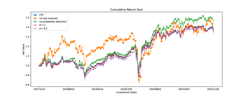
Figure 1: The cumulative returns of five optimal portfolios.

Table 4: Performance of five optimal portfolios.

Setting	Mean	Volatility	Sharpe Ratio	MD
CPT $B=0$	0.1380	0.0964	1.4314	0.3001
CPT $B=r_{f}$	0.1374	0.0965	1.4232	0.3013
$\alpha=0.5$	0.1251	0.0955	1.31	0.2883
no loss aversion	0.1851	0.1708	1.0838	0.5248
no probability distortion	0.166	0.1068	1.5536	0.2928

We conducted a thorough analysis of the performance of the optimal portfolios under various model settings. When changing the reference point from 0 to the risk-free rate $r_{f}$, the performances of the two corresponding optimal portfolios were nearly identical, as $r_{f}$ is relatively small and close to 0. When reducing the risk aversion parameter $\alpha$ from 0.88 to 0.5, the portfolio achieves the lowest mean, volatility and MD, which results in the second lowest Sharpe ratio. When reducing the loss aversion parameter $\mu$ from 2.25 to 1 resulted in the highest mean of returns, albeit at the cost of higher risk, as reflected by the highest volatility and maximum drawdown (MD) and the lowest Sharpe ratio. This finding is intuitive, as loss aversion introduces a kink around the reference point and makes the investor more risk-averse. Consequently, we further examined the case where $\mu=1$ and found that an investor without loss aversion would be less risk-averse and would opt for the riskiest portfolio among the five optimal portfolios. Finally, we evaluated the performance of the optimal portfolio with no probability distortion and found that it achieved the highest Sharpe ratio. This finding could be attributed to better diversification, which is driven by removing probability distortion. Our diversification analysis, presented below, provides further evidence supporting this argument.

Probability distortion can lead to under-diversification due to the investor’s preference for gambling, as noted by Barberis, (2013). We analyzed the diversification levels of the five optimal portfolios by examining their portfolio weights. Figure 2 shows the average weights of each portfolio on the top five assets. The weights of the “CPT $B=0$” and “CPT $B=r_{f}$” models are similar, and the “no probability distortion” and “$\alpha=0.5$” models show better diversification in terms of the weights of the top five. The “no loss aversion” model results in an extreme allocation, with heavy gambling on a single asset.

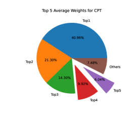
(a) CPT $B=0$

(b) CPT $B=r_{f}$

(c) $\alpha=0.5$

(d) no loss aversion

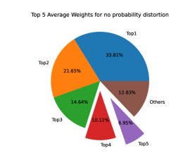
(e) no probability distortion

Figure 2: Average weights on five top assets.

In addition to comparing the portfolio weights of the five different models, we also calculate the diversification degrees of the five optimal portfolios. We followed Goetzmann and Kumar, (2008) and used the sum of squared portfolio weights (SSPW) as our metric, where SSPW is defined as follows:

$$SSPW=\sum_{i=1}^{N}\left(x_{i}-\frac{1}{N}\right)^{2}.$$

Here, $N$ is the number of assets, and $x_{i}$ is the portfolio weight assigned to asset $i$ in the portfolio. This metric measures how the portfolio weight $x_{i}$ deviates from the $1/N$ portfolio, which is seen as the best-diversified portfolio. Hence, the lower the value of SSPW, the higher the level of diversification. We computed SSPW values of the five optimal portfolios every day from 2017-12-12 to 2021-12-11 and showed the corresponding box plots in Figure 3. Figure 3(d) shows that removing probability distortion decreased the value of SSPW, thereby increasing the level of diversification. Compared with the benchmark case “CPT $B=0$”, removing probability distortion reduces the value of SSPW, therefore increasing the level of diversification. This finding is consistent with the theoretical prediction of Barberis, (2013). Figure 3(c) shows the comparison result for the “no loss aversion” and benchmark case. As expected, removing loss aversion makes the investor gamble heavily and therefore results in portfolio concentration, i.e., a large increase in terms of SSPW. Figure 3(b) shows the comparison result between $\alpha=0.5$ and $\alpha=0.88$. Increasing the risk aversion parameter and removing loss aversion have a similar effect in determining the value of SSPW. This is quite intuitive. Both increasing the risk aversion parameter and removing loss aversion make the investor less risk averse, therefore resulting in a more risky and gambling portfolio.

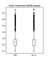
(a) CPT $B=r_{f}$

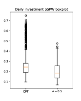
(b) $\alpha=0.5$

(c) no loss aversion

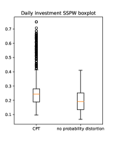
(d) no probability distrortion

Figure 3: The box-plots of five optimal portfolios’ diversification degrees.

References

- Acerbi, (2002) Acerbi, C. (2002). Spectral measures of risk: A coherent representation of subjective risk aversion. Journal of Banking & Finance, 26(7):1505–1518.
- Ahuja and Orlin, (2001) Ahuja, R. K. and Orlin, J. B. (2001). A fast scaling algorithm for minimizing separable convex functions subject to chain constraints. Operations Research, 49(5):784–789.
- Ayer et al., (1955) Ayer, M., Brunk, H. D., Ewing, G. M., Reid, W. T., and Silverman, E. (1955). An empirical distribution function for sampling with incomplete information. The Annals of Mathematical Statistics, pages 641–647.
- Bai et al., (2021) Bai, X., Sun, J., and Zheng, X. (2021). An augmented lagrangian decomposition method for chance-constrained optimization problems. INFORMS Journal on Computing, 33(3):1056–1069.
- Barberis, (2013) Barberis, N. (2013). The psychology of tail events: Progress and challenges. American Economic Review, 103(3):611–16.
- Barberis and Huang, (2008) Barberis, N. and Huang, M. (2008). Stocks as lotteries: The implications of probability weighting for security prices. American Economic Review, 98(5):2066–2100.
- Barberis and Xiong, (2009) Barberis, N. and Xiong, W. (2009). What drives the disposition effect? An analysis of a long-standing preference-based explanation. Journal of Finance, 64(2):751–784.
- Bazaraa et al., (2006) Bazaraa, M. S., Sherali, H. D., and Shetty, C. M. (2006). Nonlinear programming: theory and algorithms. John Wiley & Sons.
- Beck, (2017) Beck, A. (2017). First-order methods in optimization. SIAM.
- Bernard and Ghossoub, (2010) Bernard, C. and Ghossoub, M. (2010). Static portfolio choice under cumulative prospect theory. Mathematics and Financial Economics, 2(4):277–306.
- Best and Chakravarti, (1990) Best, M. J. and Chakravarti, N. (1990). Active set algorithms for isotonic regression; a unifying framework. Mathematical Programming, 47(1):425–439.
- Best et al., (2000) Best, M. J., Chakravarti, N., and Ubhaya, V. A. (2000). Minimizing separable convex functions subject to simple chain constraints. SIAM Journal on Optimization, 10(3):658–672.
- Boyd et al., (2011) Boyd, S., Parikh, N., Chu, E., Peleato, B., Eckstein, J., et al. (2011). Distributed optimization and statistical learning via the alternating direction method of multipliers. Foundations and Trends® in Machine Learning, 3(1):1–122.
- Brunk et al., (1972) Brunk, H., Barlow, R. E., Bartholomew, D. J., and Bremner, J. M. (1972). Statistical inference under order restrictions:the theory and application of isotonic regression. John Wiley & Sons.
- Clarke, (1990) Clarke, F. H. (1990). Optimization and nonsmooth analysis. SIAM.
- Combettes and Pesquet, (2007) Combettes, P. L. and Pesquet, J.-C. (2007). A douglas–rachford splitting approach to nonsmooth convex variational signal recovery. IEEE Journal of Selected Topics in Signal Processing, 1(4):564–574.
- Cui et al., (2018) Cui, X., Sun, X., Zhu, S., Jiang, R., and Li, D. (2018). Portfolio optimization with nonparametric value at risk: A block coordinate descent method. INFORMS Journal on Computing, 30(3):454–471.
- Cui et al., (2021) Cui, Z., Lee, C., Zhu, L., and Zhu, Y. (2021). Non-convex isotonic regression via the myersonian approach. Statistics & Probability Letters, 179:109210.
- De Giorgi and Legg, (2012) De Giorgi, E. and Legg, S. (2012). Dynamic portfolio choice and asset pricing with narrow framing and probability weighting. Journal of Economic Dynamics & Control, 36(7):951–972.
- Dhaene et al., (2006) Dhaene, J., Vanduffel, S., Goovaerts, M. J., Kaas, R., Tang, Q., and Vyncke, D. (2006). Risk measures and comonotonicity: a review. Stochastic models, 22(4):573–606.
- Duffie and Pan, (1997) Duffie, D. and Pan, J. (1997). An overview of value at risk. Journal of derivatives, 4(3):7–49.
- Glowinski and Marrocco, (1977) Glowinski, R. and Marrocco, A. (1977). Numerical solution of two-dimensional magnetostatic problems by augmented lagrangian methods. Computer Methods in Applied Mechanics and Engineering, 12(1):33–46.
- Goetzmann and Kumar, (2008) Goetzmann, W. N. and Kumar, A. (2008). Equity portfolio diversification. Review of Finance, 12(3):433–463.
- He and Zhou, (2011) He, X. D. and Zhou, X. Y. (2011). Portfolio choice under cumulative prospect theory: An analytical treatment. Management Science, 57(2):315–331.
- Jin and Zhou, (2008) Jin, H. and Zhou, X. Y. (2008). Behavioral portfolio selection in continuous time. Mathematical Finance, 18(3):385–426.
- Kahneman and Tversky, (1979) Kahneman, D. and Tversky, A. (1979). Prospect theory: An analysis of decisions under risk. Econometrica, 47:263–291.
- Levy and Levy, (2004) Levy, H. and Levy, M. (2004). Prospect theory and mean-variance analysis. Review of Financial Studies, 17(4):1015–1041.
- Li et al., (2015) Li, X., Wang, W., Xu, C., Li, Z., and Wang, B. (2015). Multi-objective optimization of urban bus network using cumulative prospect theory. Journal of Systems Science and Complexity, 28(3):661–678.
- Liu et al., (2013) Liu, W., Liu, C., and Ge, M. (2013). An order allocation model for the two-echelon logistics service supply chain based on cumulative prospect theory. Journal of Purchasing and Supply Management, 19(1):39–48.
- Luxenberg et al., (2022) Luxenberg, E., Schiele, P., and Boyd, S. (2022). Portfolio optimization with cumulative prospect theory utility via convex optimization. arXiv preprint arXiv:2209.03461.
- Nagarajan and Shechter, (2014) Nagarajan, M. and Shechter, S. (2014). Prospect theory and the newsvendor problem. Management Science, 60(4):1057–1062.
- Nocedal and Wright, (1999) Nocedal, J. and Wright, S. J. (1999). Numerical optimization. Springer.
- Quiggin, (2012) Quiggin, J. (2012). Generalized expected utility theory: The rank-dependent model. Springer Science & Business Media.
- Rockafellar et al., (2000) Rockafellar, R. T., Uryasev, S., et al. (2000). Optimization of conditional value-at-risk. Journal of risk, 2:21–42.
- Rockafellar and Wets, (2009) Rockafellar, R. T. and Wets, R. J.-B. (2009). Variational analysis, volume 317. Springer Science & Business Media.
- Scheinberg et al., (2010) Scheinberg, K., Ma, S., and Goldfarb, D. (2010). Sparse inverse covariance selection via alternating linearization methods. Advances in neural information processing systems, 23.
- Shen et al., (2014) Shen, Y., Wen, Z., and Zhang, Y. (2014). Augmented lagrangian alternating direction method for matrix separation based on low-rank factorization. Optimization Methods and Software, 29(2):239–263.
- (38) Shi, Y., Cui, X., and Li, D. (2015a). Discrete-time behavioral portfolio selection under cumulative prospect theory. Journal of Economic Dynamics & Control, 61:283–302.
- (39) Shi, Y., Cui, X., Yao, J., and Li, D. (2015b). Dynamic trading with reference point adaptation and loss aversion. Operations Research, 63(4):789–806.
- Srivastava et al., (2022) Srivastava, S., Aggarwal, A., and Mehra, A. (2022). Portfolio selection by cumulative prospect theory and its comparison with mean-variance model. Granular Computing, pages 1–14.
- Strömberg, (1991) Strömberg, U. (1991). An algorithm for isotonic regression with arbitrary convex distance function. Computational Statistics & Data Analysis, 11(2):205–219.
- Tversky and Kahneman, (1992) Tversky, A. and Kahneman, D. (1992). Advances in prospect theory: Cumulative representation of uncertainty. Journal of Risk and Uncertainty, 5(4):297–323.
- van Bilsen and Laeven, (2020) van Bilsen, S. and Laeven, R. J. (2020). Dynamic consumption and portfolio choice under prospect theory. Insurance: Mathematics and Economics, 91:224–237.
- Xu et al., (2012) Xu, Y., Yin, W., Wen, Z., and Zhang, Y. (2012). An alternating direction algorithm for matrix completion with nonnegative factors. Frontiers of Mathematics in China, 7(2):365–384.
- Yu et al., (2022) Yu, Z., Chen, X., and Li, X. (2022). A dynamic programming approach for generalized nearly isotonic optimization. Mathematical Programming Computation, pages 1–31.