The high-ionization IR fine-structure lines as bolometric indicators of the AGN power:
study of the complete 12$\mu$m AGN sample

Abstract

The high-ionization mid-IR lines, excited in the Narrow Line Regions (NLR) of Active Galactic Nuclei (AGN), barely affected by stellar excitation and dust extinction, trace the AGN bolometric power. We used the complete 12$\rm{\micron}$ sample of Seyfert galaxies, for which 100/116 objects have reliable 2-10keV observations. The [NeV] and [OIV] mid-IR lines linearly correlate with several AGN bolometric indicators (intrinsic 2–10keV and observed 14–195keV X-ray emission, compact nuclear 12$\rm{\micron}$ emission, [OIII] $\lambda$5007Å  line emission), both in terms of flux and luminosity. No evidence of systematic differences in these correlations is found among the Seyfert populations, including type 1 and type 2, and Compton thick and thin AGN. Nevertheless, we find that a sequence of high-to-low Eddington ratio together with strong-to-weak line excitation (traced by the [OIV]/[Ne II] line ratio) encompasses from type 1 through type 2 AGN to Low Ionization Nuclear Emission Line Region (LINER) galaxies, showing intrinsic differences in these three AGN populations. A positive correlation between the Black Hole Accretion Rate (BHAR) and the Star Formation Rate (SFR) is found, but no correlation between the specific SFR (sSFR) and the ratio BHAR/M_BH, simply reflecting the fact that the more massive is a galaxy, the more it is forming stars and feeding its central black hole. The JWST telescope, just beginning operations, will allow large samples of AGN to be observed in these lines in the nearby Universe (z$<$0.9).

1 Introduction

A full understanding of galaxy evolution still needs both observational and theoretical efforts. While our theoretical understanding of complex baryonic processes is advancing (see, e.g. Wechsler & Tinker, 2018), there still remains a large gap in comparing theory with currently limited observations. Rest-frame optical and UV data are used to probe star formation in distant galaxies, but are greatly affected by dust. X-ray data are sensitive tracers of black hole activity, but are often limited by sensitivity and resolution. In the most obscured regions, such as those at the centers of forming galaxies, all but the highest energy X-rays can be absorbed. It has become evident during the last few decades that the key phases of galaxy evolution – the birth and growth of stars and the growth of supermassive black holes (SMBH) – take place within regions enshrouded in dust, largely hidden from view at optical and UV wavelengths (Madau & Dickinson, 2014) and suffering from the effects of obscuration at X-ray energies (see, e.g. Compton thick objects with hydrogen column densities in excess of 10²⁴ cm^-2; Bassani et al. 1999; Del Moro et al. 2016). The observed evolution of star formation and black hole growth over cosmic time appear remarkably similar, with a peak around z$\sim$2 and then decreasing by a factor of 30 in the last 10 Gyrs. At this peak, an epoch known as cosmic noon, nearly 90% of the energy emitted by young stars emerges in the infrared from dust, re-radiating the energy absorbed from young stars and growing supermassive black holes (Goto et al., 2019). The infrared spectrum therefore provides a critical window through which we can understand the crucial hidden part of galaxy evolution, and measure both the star formation rate (SFR) and the black hole accretion rate (BHAR) in individual galaxies over much of cosmic time.

This work aims to establish what are the best IR tracers for black hole accretion, and for star formation (to be able to separate the two components), in the local Universe. These can then be used at intermediate redshift by JWST (z$<$0.9) and have the potential to be used at high redshift (z$\lesssim$3.5) by the upcoming IR space telescopes of the next decade(s), for studying galaxy evolution. A suitable laboratory to study the interplay of black hole accretion and star formation, which is fundamental to the evolution of galaxies, is given in the local Universe by the class of the Seyfert galaxies, which are powered by both black hole accretion in their nuclei and also by star formation, either circum-nuclear ( at physical scales up to $\sim$200 pc for circumnuclear disks) and/or in the galaxy disk (at scales of $\sim$1-10 kpc).

The mid-infrared (mid-IR) spectra of Seyfert galaxies are very rich in narrow emission lines that can be powered by both the presence of active galactic nuclei (AGN) and star formation occurring in circumnuclear regions and in the galactic disk (see, e.g. Tommasin et al. 2008, 2010). The potential of the IR line diagnostics was first demonstrated by Spinoglio & Malkan (1992). Unlike optical spectroscopy, mid-IR spectroscopy is much less affected by dust extinction, as can be quantified by the fact that 50 mag of extinction in the V-band corresponds to only 1 mag at 24$\mu$m (e.g., Genzel et al., 1998). Thus, infrared observations are the only practical tool for spectroscopically studying dust-obscured galaxies and AGN. The brightest AGN features in the mid-IR range are the high-ionization forbidden emission lines from [NeV] at 14.3 and 24.3$\mu$m and [OIV] at 25.9$\mu$m. Given its high ionization potential (IP = 97 eV), Ne⁴⁺ is an unambiguous tracers of the AGN narrow-line region (NLR), whereas O³⁺ (IP = 54.9 eV) is dominated by the AGN contribution, with an equivalent width of about a factor ten higher compared to Starburst galaxies (Sturm et al., 2002; Meléndez et al., 2008; Tommasin et al., 2008, 2010). The star-formation tracers include the strong PAH emission features (at, e.g., 11.3$\mu$m), the mid-IR pure rotational lines of H₂ and the low-ionization fine-structure lines (e.g. [NeII]12.8$\mu$m, with IP=21.6eV, [SIII]18 and 33$\mu$m, IP = 23.3eV, and [SiII]34.8$\mu$m, IP = 16.3eV), as well as the ubiquitous [CII]158$\mu$m line ( IP = 11.3eV) (see, e.g. De Looze et al., 2011, 2014). We refer to Mordini et al. (2021, 2022) for a detailed recent calibration of the fine-structure lines luminosities against the total IR luminosities.

On the other hand, the hard X-ray emission in the $2$–$10\,\rm{keV}$ band is a direct measure of the current (instantaneous) accretion luminosity for all AGNs except the extreme Compton thick objects. For Compton-thin sources ($\rm{N_{H}}\lesssim 10^{24}\,\rm{cm^{-2}}$) a correction can be applied to recover a reliable intrinsic luminosity (see, e.g., Ricci et al., 2015). The higher energy continuum (e.g. $14$–$195\,\rm{keV}$) can be used in some cases to measure the nuclear continuum in Compton-thick sources. The relationship between the accretion luminosity, as derived from the X-rays, and the NLR luminosity, measured by the high-ionization mid-IR fine structure lines of [NeV] and [OIV], can shed light on the differences between the three main types of active galaxies. The NLR emission, especially if traced by long-wavelength transitions, is thought to be essentially isotropic, because the spatial scale of the NLR ($100$–$500\,\rm{pc}$) is much larger than the predicted size of the obscuring dust tori. These latter are expected to be of the order of a few parsecs in size (see, e.g. Jaffe et al., 2004; Elitzur & Shlosman, 2006; Tristram et al., 2007; Pott et al., 2010).

Previous studies have found intrinsic differences in the X-ray to NLR line ratios between Seyfert 1 and 2, ascribed to obscuration affecting the observed hard X-ray fluxes (up to the 14–195 keV band) and the optical NLR emission in type 2 nuclei (Meléndez et al., 2008; Rigby et al., 2009; LaMassa et al., 2010). However, this is in contrast with the indistinguishable [OIV] luminosity distributions of both Seyfert classes (Diamond-Stanic et al., 2009; Tommasin et al., 2010).

In this work, instead of using X-ray or optically selected samples of Seyfert galaxies, we use the complete $12\,\rm{\micron}$ selected sample of Seyfert galaxies (Rush et al., 1993), exploiting the large set of multi-frequency data available, to better understand the nature of the “pure” Seyfert 2’s and how they are related to type 1’s. For example, are they intrinsically the same, and can they be related through a simple unification, such as viewing angle? Or are AGN intrinsically different? Furthermore, we have studied the relation between the host galaxy properties and those of the AGN, comparing these galaxies with the so-called Main-Sequence of star forming galaxies (Elbaz et al., 2011).

Taking advantage of the complete and virtually unbiased galaxy sample that we use, we have studied: (i) the correlation between the bolometric luminosity as derived from X-rays observations and that one derived from the high-ionization [O IV] 25.89 $\mu$m  line; (ii) the differences in the accretion process among the various AGN spectroscopic classes; (iii) the relation between the AGN properties (BHAR, Eddington ratio) and those of the host galaxy (M$\star$, SFR, sSFR).

The paper is organized as follows: section 2 describes the sample of AGN used; section 3 gives the major results of this paper and is divided into the following parts: 3.1 gives the correlations between the X-ray emission and the mid-IR fine structure lines; 3.3 shows the correlations between the X-ray emission and both the [O III] 5007 Å  optical line and the 12$\mu$m nuclear continuum; 3.5 shows how the X-ray and mid-IR determinations of the AGN bolometric luminosity agree; 3.6.1 shows the LED diagram for our sample; 3.6.2 shows the Eddington ratio as a function of the bolometric luminosity; 3.4 shows the correlation between the [O IV] 25.89 $\mu$m  and [O III] 5007 Å  line fluxes and luminosities and finally 3.7.2 gives the correlation between SFR and BHAR. Finally in section 4 the various results are compared with previous studies.

2 The sample

Our study is based on the $12\,\rm{\micron}$ Seyfert galaxy sample (53 Seyfert 1’s and 63 Seyfert 2’s) (hereafter 12MSG) extracted from the Infrared Astronomical Satellite (IRAS) $12\,\rm{\micron}$ galaxy sample (Rush et al., 1993). The chosen sample is essentially a bolometric flux-limited survey outside the galactic plane, and therefore largely unbiased, given the empirical fact that galaxies emit an approximately constant fraction of their total bolometric luminosity at $12\,\rm{\micron}$. This fraction is $\sim 15\%$ for AGNs (Spinoglio & Malkan, 1989) and $7\%$ for normal and starburst galaxies, independent of star formation activity (Spinoglio et al., 1995).

The multi-frequency observations that we use in our analysis include the hard X-rays observations in the bands $2$–$10\,\rm{keV}$ and $14$–$195\,\rm{keV}$ from Ricci et al. (2017a) and Oh et al. (2018), which include the broadband X-ray ($0.3$–$150\,\rm{keV}$) characteristics of the BAT-detected AGNs, obtained by combining XMM-Newton, Swift/XRT, ASCA, Chandra, and Suzaku observations in the soft X-ray band, in addition to the Swift-BAT AGN 70 months catalog. We also use the optical spectroscopy from Malkan et al. (2017) and the 12$\mu$m nuclear fluxes from Asmus et al. (2014), as well as the Spitzer spectroscopic data (Tommasin et al., 2008; Wu et al., 2009; Gallimore et al., 2010; Tommasin et al., 2010) and the Herschel PACS spectra (Fernández-Ontiveros et al., 2016).

Using the optical spectropolarimetric results that have been extensively obtained for the $12\,\rm{\micron}$ selected Seyfert sample (Tran, 2003, and references therein), Tommasin et al. (2010) have proposed a classification of Seyfert galaxies, dividing them into the three classes: Seyfert type 1’s (hereafter Sy1), Hidden Broad Line Seyfert type 2’s (hereafter HBL), showing the presence of broad lines in polarized light, and “pure” Seyfert type 2’s (hereafter Sy2), without any sign of detected broad emission lines. The infrared spectral behavior of the Sy1 and HBL is indistinguishable, implying that they indeed belong to the larger class of “type 1” AGNs. Sy2 are not a homogeneous class–some of them have properties similar to type 1’s, and may include a fraction of undetected type 1 nuclei, while others are more similar to non-Seyfert galaxies, either starburst or Low Ionization Nuclear Emission Regions (LINERs) (see, e.g. Ho et al., 1997).

The 12MSG sample has complete observational coverage at virtually every wavelength, from radio to hard X-rays (see Tommasin et al., 2008, for a review up to 2008) and Wu et al. (2009); Baum et al. (2010); Tommasin et al. (2010); Gallimore et al. (2010); LaMassa et al. (2010); Brightman & Nandra (2011); Pereira-Santaella et al. (2013); Spinoglio et al. (2015); Theios et al. (2016); Gruppioni et al. (2016); Gómez-Guijarro et al. (2017); Malkan et al. (2017); La Caria et al. (2019).

Table LABEL:tab:sample0 lists the galaxies of the full AGN sample selected from the revised 12$\mu$m sample of galaxies (Rush et al., 1993) with the galaxy coordinates, redshift and activity type based on optical spectroscopy. Table LABEL:tab:sample1 gives for each galaxy the X-ray data information, where available, including the derived hydrogen column density, whether the galaxy is Compton thick (CT), the SWIFT identification, where available, the (2-10)KeV intrinsic, i.e. absorption corrected, X-ray flux and luminosity, the (14-195)KeV X-ray flux and luminosity (Oh et al., 2018; Ricci et al., 2017a; Cusumano et al., 2010) and the bolometric luminosity as derived from the (2-10)keV intrinsic luminosity, and the bolometric correction from Lusso et al. (2012). Table 6 lists the Compton thick objects of our sample with the observed and corrected (2-10)keV fluxes and luminosities and the bolometric luminosities as derived from these X-ray fluxes.

Table LABEL:tab:sample2 gives the fluxes of the emission lines considered in this study: the [NeII]12.8$\mu$m, [NeV]14.32$\mu$m, [NeII]15.5$\mu$m, [NeV]24.32$\mu$m and [OIV]25.89$\mu$m mid-IR fine structure lines from Tommasin et al. (2008, 2010), the [CII]158$\mu$m line from Fernández-Ontiveros et al. (2016) and the [OIII]5007Å optical line flux from Malkan et al. (2017). We include the 12$\mu$m nuclear flux density from Asmus et al. (2014).

The Spitzer IRS spectrograph apertures used for the fine structure lines were 4.7” $\times$ 11.3” for the short wavelength lines ([Ne II] 12.81 $\mu$m, [Ne III] 15.55 $\mu$m and [NeV] 14.32 $\mu$m) and 11.1” $\times$ 22.3” for the long wavelength lines ([NeV] 24.32 $\mu$m, [O IV] 25.89 $\mu$m). Given the average redshift of the 12MSG active galaxies of z=0.028 (Rush et al., 1993), which corresponds to a mean distance of 124.5 Mpc, ($H_{0}=67.4\,\rm{km\,s^{-1}\,Mpc^{-1}}$) the short and long wavelength apertures of the Spitzer IRS spectrograph correspond to a linear area of $\sim 1\,\rm{kpc}$ and 5 kpc in diameter, respectively. Therefore the NLRs of our sample of AGN are – on average – fully covered by the mid-IR spectroscopic observations.

Since the goal of our spectroscopy is to measure line emission produced by the AGN, our optical line measurements typically refer to the central several arcseconds of the galaxy. The smallest apertures used in Malkan et al. (2017) were the SDSS (York et al., 2000) fibers (3” diameter) while the largest apertures (typically rectangular slits) were roughly twice that size (a few kpc). The line emission from these relatively small regions is strongly dominated by the NLR powered by the AGN, with only minor contributions from H ii regions in the disk of the host spiral galaxy (Theios et al., 2016; Xia et al., 2018). Conversely, for the closest Seyfert galaxies, it is possible that extended NLR emission from the AGN could extend beyond 1 kpc from the nucleus. Fortunately even in the most extreme known cases the [OIII] line emission powered by the AGN is compact, nearly all of it confined within $\sim 700\,\rm{pc}$ from the central nucleus (Schmitt & Kinney, 1996).

Table LABEL:tab:sample3 gives the K-band photometry of each of the observed galaxies: the estimated total and nuclear K-band flux densities, derived from the 2MASS Extended Source Catalog, the estimated stellar mass of the galaxy, the bolometric luminosity as derived from the [OIV]25.89$\mu$m, using the calibration of Mordini et al. (2021) with the bolometric correction of Spinoglio et al. (1995), and the supermassive black hole mass, as derived mostly from stellar velocity dispersion observations that can be found in Fernández-Ontiveros & Muñoz-Darias (2021, and references therein). The galaxy flux has been derived starting from the total 2MASS XSC flux (called “$K\_mag\_ext^{\prime}"$, which uses the extrapolation of the surface brightness model fit to the data, integrated over the entire object). From this total luminosity, we then subtract the non-stellar nuclear component. We estimate this from either high spatial resolution K-band observations (Keck/OSIRIS with adaptive optics) (Müller-Sánchez et al., 2018) or by using the “peak” H and K magnitudes given in the 2MASS XSC. For 19 AGN (see Table LABEL:tab:sample3), for which HST observations have been used to compute the R-band absolute magnitudes of the host galaxy (Kim et al., 2017), through image decomposition using the code GALFIT (Peng et al., 2002), we have adopted the stellar masses as derived from the relation between R-absolute magnitude and stellar mass of Mahajan et al. (2018), who used a sample of 428 galaxies in the redshift range 0.002 $<$ z $<$ 0.02, with MAGPHYS (da Cunha et al., 2008) fits of the 21-band photometry from Driver et al. (2016).

In each table the AGN have been divided in four classes: Seyfert type 1 galaxies, Hidden Broad Line Region galaxies (hereafter HBL), Seyfert type 2 galaxies and LINER galaxies (hereafter LIN). The inclusion of the HBL galaxies follows the work by Tommasin et al. (2010), who found that the mid-IR spectroscopic properties of the HBL are indistinguishable from those of the type 1 Seyfert galaxies, and the optical spectropolarimetry that has been collected primarily by Tran (2003).

3 Results

3.1 The X-ray/mid-IR lines correlation

In this study we have considered that, in order to establish a physical link between two quantities (either emission line or continuum strengths) a significant correlation has to be found between their fluxes, because correlations based only on the luminosities are not reliable enough. This is because the luminosity correlations are boosted by the distance squared factor, which may produce a spurious trend from uncorrelated fluxes. Nevertheless, our results will be mostly compared with luminosity correlations in the literature, since few studies discuss the flux correlations.

To study the relationship between the bolometric continuum of the AGN and the luminosity emitted from the NLR and powered by the accretion activity (hereafter, X–mid-IR relation), we analyzed the hard X-ray $2$–$10\,\rm{keV}$ intrinsic (i.e. absorption-corrected) flux and luminosity as a function of the three high-ionization mid-IR fine-structure NLR emission lines ([NeV] 14.32 $\mu$m, [NeV] 24.32 $\mu$m and [OIV] 25.89 $\mu$m. The latter requirement guarantees that most of the energy carried by these lines originates from accretion processes rather than star formation, while the mid-IR wavelength region allows us to neglect dust extinction of the line fluxes. For comparison, we also included in the analysis the lower ionization lines of [NeIII]15.5 $\mu$m (IP = 40.9eV) and [NeII]12.8 $\mu$m. The former is excited by both the AGN and the star-forming component of the galaxy and the latter mostly by the star-forming component (Spinoglio & Malkan, 1992).

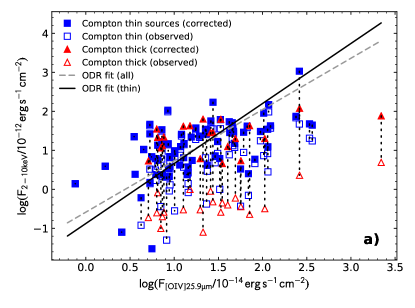
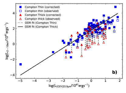
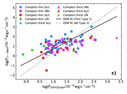
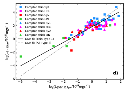
Figure 1: a: upper left X-ray (2–10) keV intrinsic flux as a function of the [O IV] 25.9$\mu$m line flux for all sources with reliable hard-X data and an optical spectroscopic classification. The blue squares indicate the Compton-thin AGN, while Compton- thick objects are denoted by red triangles. The solid lines represent the linear regression fit with all objects, while the dotted line shows the fit to only Compton-thin objects (see Table 1). b: upper right X-ray (2-10) keV intrinsic luminosity vs. [O IV] line luminosity (both in logarithmic units of erg s^-1). c: lower left Same as a, but with the objects color coded: Seyfert types 1 (Sy1): blue; Hidden Broad Line Region Galaxies (HBL): magenta; Seyfert types 2 (Sy2): red; LINERS (LIN): green. The solid line shows the fit for all Compton-thin Type 1 AGN, which include both Seyfert 1’s and HBL, while the broken line gives the bet fit for all the Type 2 objects, i.e. the pure Seyfert 2’s, both Compton- thick and thin (see Table 1). d: lower right Same as b, but with the objects color coded, according to panel c. The fits are similar to those in panel c, but between luminosities (see Table 1).

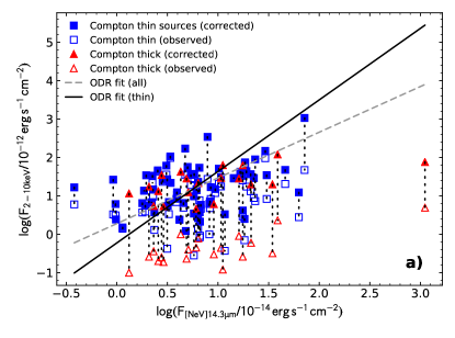
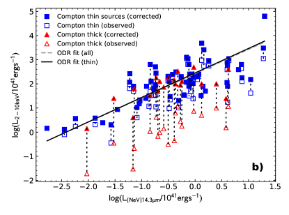
Figure 2: a: left X-ray (2–10) keV intrinsic flux as a function of the [NeV] 14.3$\mu$m line flux for all sources with reliable hard-X data and an optical spectroscopic classification. The blue squares indicate the Compton-thin AGN, while Compton-thick objects are denoted by red triangles. The solid lines represent the linear regression fit with all objects, while the dotted line the fit with only Compton-thin objects. b: right X-ray (2-10) keV intrinsic luminosity vs. [NeV] line luminosity (both in logarithmic units of erg s^-1).

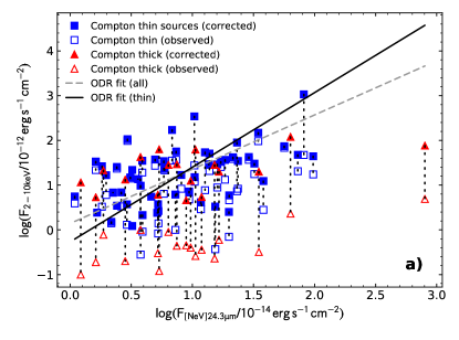
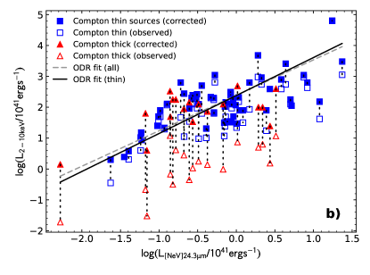
Figure 3: a: left X-ray (2–10) keV intrinsic flux as a function of the [NeV] 24.3$\mu$m line flux for all sources with reliable hard-X data and an optical spectroscopic classification. The blue squares indicate the Compton-thin AGN, while Compton-thick objects are denoted by red triangles. The solid lines represent the linear regression fit with all objects, while the dotted line the fit with only Compton-thin objects. b: right X-ray (2-10) keV intrinsic luminosity vs. [NeV] 24.3$\mu$m line luminosity (both in logarithmic units of erg s^-1).

To quantify the statistical significance of these relations, we used a orthogonal distance regression (ODR) fit. The results are presented in Table 1, where the Pearson linear correlation coefficients are shown for the flux and luminosity relations for each of the five considered mid-IR fine structure lines, together with the linear regression best-fit parameters with relative uncertainties. All correlations have been computed for the whole population of AGN and for the sub-sample of Compton-thin objects (C-thin). For the particular case of the [OIV]25.9$\mu$m line, because of the higher statistics compared to the other lines, also the correlations of the sub-sample of Type 1 objects, which include all the Compton-thin Seyfert type 1 and HBL galaxies, have been computed and compared to the Type 2 objects, which include ”pure” Seyfert type 2 galaxies (see Table 1).

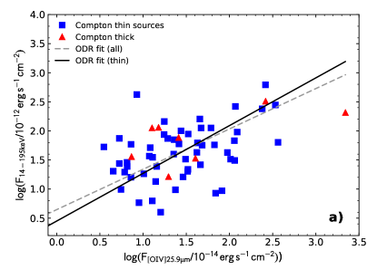
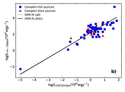
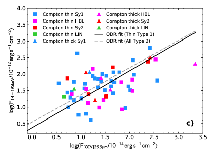
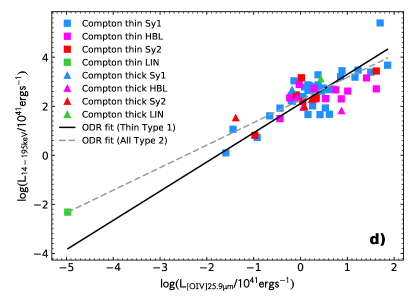
Figure 4: a: left X-ray (14-195) keV intrinsic flux as a function of the [O IV] 25.9$\mu$m line flux for all sources with reliable hard-X data and an optical spectroscopic classification. The blue squares indicate the Compton-thin AGN, while Compton-thick objects are denoted by red triangles. The solid lines represent the linear regression fit with all objects, while the dotted line the fit with only Compton-thin objects . b: right X-ray (14-195) keV intrinsic luminosity vs. [O IV] line luminosity (both in logarithmic units of erg s^-1). c: lower left Same as a, but with the objects color coded: Seyfert types 1 (Sy1): blue; Hidden Broad Line Region Galaxies (HBL): magenta; Seyfert types 2 (Sy2): red; LINERS (LIN): green. d: lower right Same as b, but with the objects color coded, according to panel c.

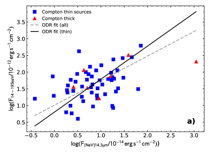
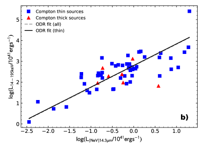
Figure 5: a: left X-ray (14-195) keV intrinsic flux as a function of the [NeV] 14.3$\mu$m line flux for all sources with reliable hard-X data and an optical spectroscopic classification. The blue squares indicate the Compton-thin AGN, while Compton-thick objects are denoted by red triangles. The solid lines represent the linear regression fit with all objects, while the dotted line the fit with only Compton-thin objects. b: right X-ray (14-195) keV intrinsic luminosity vs. [NeV] 14.3$\mu$m line luminosity (both in logarithmic units of erg s^-1).

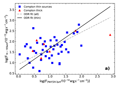
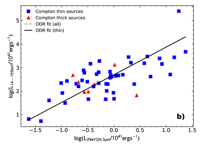
Figure 6: a: left X-ray (14-195) keV intrinsic flux as a function of the [NeV] 24.3$\mu$m line flux for all sources with reliable hard-X data and an optical spectroscopic classification. The blue squares indicate the Compton-thin AGN, while Compton-thick objects are denoted by red triangles. The solid lines represent the linear regression fit with all objects, while the dotted line the fit with only Compton-thin objects. b: right X-ray (14-195) keV intrinsic luminosity vs. [NeV] 24.3$\mu$m line luminosity (both in logarithmic units of erg s^-1).

In Figure 1 the hard X-ray ($2$–$10)\,\rm{keV}$ observed (open symbols) and intrinsic (i.e. absorption-corrected) fluxes (panel a) and luminosities (panel b) of both the Compton-thin and the Compton-thick AGN are plotted as a function of the flux and luminosity, respectively, of the [O IV] 25.9$\mu$m line for the subsample of the 12MSG with reliable hard X-ray data obtained from the literature. The observed and corrected X-ray fluxes and luminosities are connected in the diagrams by a broken line, which indicates the correction applied either by fitting the X-ray spectra or by extrapolating the X-ray ($14$–$195)\,\rm{keV}$ flux and luminosity to the ($2$–$10)\,\rm{keV}$ band (see, e.g., Ricci et al., 2017a). In the same Fig. 1, panels c and d show the intrinsic fluxes and luminosities, respectively, but with the color coded types of AGN, which are divided in the four classes of Seyfert 1’s (Sy1), Hidden Broad Line region galaxies (HBL), Seyfert 2’s (Sy2) and LINER (LIN).

Figures 2 and 3 show the ($2$–$10)\,\rm{keV}$ observed and intrinsic fluxes (panel a) and luminosities (panel b) versus that of the [NeV] 14.3$\mu$m line and [NeV] 24.3$\mu$m line, respectively.

It is clear from the three figures 1, 2 and 3 that to derive a reliable relation between the X-ray and mid-IR line fluxes and luminosities it is mandatory to correct the X-ray data, as the application of absorption corrections reduces the scatter of the data points by a large amount. We do not even try to compute correlations using the observed ($2$–$10)\,\rm{keV}$ X-ray fluxes.

To demonstrate that the higher ionization lines of [NeV] and [O IV] are the best tracers of AGN emission, we also show in Fig. 18 and 19 in the Appendix the same plots between the ($2$–$10)\,\rm{keV}$ observed and intrinsic fluxes (panel a) and luminosities (panel b) and the [Ne III] 15.55 $\mu$m and [Ne II] 12.81 $\mu$m lines.

Examining the results of the orthogonal distance regression (ODR) fits, shown in Table 1, it is clear that the best flux correlation is obtained for the [O IV] 25.9$\mu$m line, followed by the [NeV]24.3$\mu$m and [NeV]14.3$\mu$m. The slope of the correlation for these three mid-IR fine structure lines is of the order of $B=1.2-1.4$ and becomes relatively steeper $B=1.6-1.8$ when considering only the Compton-thin AGN, instead of the total observed population. The [Ne III] 15.55 $\mu$m  line has a relatively high value of the Pearson coefficient (R$\sim$0.47, n=100), however the slope is abnormally high ($B=2.7-3.5$). To the contrary, no correlation is apparent between the [Ne II] 12.81 $\mu$m  line and the X-ray flux.

In analogy with Fig.1, Fig.4 shows the higher energy X-ray ($14$–$195)\,\rm{keV}$ fluxes (panel a) and luminosities (panel b) of both the Compton-thin and the Compton-thick AGN as a function of the flux and luminosity, respectively, of the [O IV] 25.9$\mu$m line. In the same Fig. 4, panels c and d show the intrinsic fluxes and luminosities, respectively, but with the color coded types of AGN. In the following figures, i.e. Fig. 5, 6 and Fig. 20, 21 in the Appendix, the X-ray ($14$–$195)\,\rm{keV}$ flux and luminosity is plotted as a function of the [NeV]14.3$\mu$m, [NeV]24.3$\mu$m, [Ne II] 12.81 $\mu$m  and [Ne III] 15.55 $\mu$m  fluxes and luminosities, respectively.

The ODR fits results, given in Table 1, show that for the [O IV]  and [NeV]  lines the slope is significantly flatter than unity ($B\sim 0.7$) if all AGN are considered, but it becomes close to unity ($B=0.8-1.0$) when only Compton-thin objects are included. This is also true for the lower-ionization [Ne III] 15.55 $\mu$m  line and in most cases the correlations are relatively strong (i.e. with a $P_{null}$ probability below 10^-2). The case of [Ne II] 12.81 $\mu$m , as already seen for the lower energy X-ray band of ($2$–$10)\,\rm{keV}$, shows the weakest correlation.

Considering the correlations between the luminosities of either ($2$–$10)\,\rm{keV}$ and ($14$–$195)\,\rm{keV}$ bands and the mid-IR fine-structure line luminosities, as can be seen from either the figures and Table 1, these are always very strong and are almost linear (with a slope of $B=1.0-1.3$). This is not surprising, because luminosity-luminosity correlations are boosted by the 4$\pi$R² factor, where R is the distance of galaxy, and therefore they do not necessarily mean that the observed physical quantities are indeed correlated. We consider here that a real physical correlation must appear also between the observed (or corrected, in the case of the ($2$–$10)\,\rm{keV}$ X-ray band) fluxes and the considered emission line.

3.2 The AGN bolometric luminosities as a function of the [O IV]  and [NeV]  line luminosities

We have computed the AGN bolometric luminosities, using the Lusso et al. (2012) bolometric correction and the corrected (2-10)keV luminosities, as a function of the luminosities of the three mid-IR high ionization lines of [O IV] 25.89 $\mu$m, [NeV] 14.32 $\mu$m  and [NeV] 24.32 $\mu$m. The correlations are shown in Fig. 7(a, b, and c) and are tabulated in Table 2.

The following formulae can be used when one wants to compute the AGN bolometric luminosity from the luminosities of these lines:

$$\begin{split}\log\left(\frac{\rm L_{BOL}}{\rm 10^{41}\,erg\,s^{-1}}\right)=(3.02\pm 0.06)\\ +(0.88\pm 0.06)\log\left(\frac{L_{\rm[OIV]25.9{\mu}m}}{\rm 10^{41}\,erg\,s^{-1}}\right),\end{split}$$ (1)

$$\begin{split}\log\left(\frac{\rm L_{BOL}}{\rm 10^{41}\,erg\,s^{-1}}\right)=(3.53\pm 0.07)\\ +(0.90\pm 0.08)\log\left(\frac{\rm L_{[NeV]14.3{\mu}m}}{\rm 10^{41}\,erg\,s^{-1}}\right),\end{split}$$ (2)

$$\begin{split}\log\left(\frac{\rm L_{BOL}}{\rm 10^{41}\,erg\,s^{-1}}\right)=(3.50\pm 0.07)\\ +(1.06\pm 0.10)\log\left(\frac{\rm L_{[NeV]24.3{\mu}m}}{\rm 10^{41}\,erg\,s^{-1}}\right),\end{split}$$ (3)

The RMS scatter in these correlations is of the order of $\sim$0.3 dex, meaning that an emission line measurement can predict the AGN bolometric luminosity to an accuracy of about a factor two.

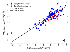
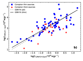
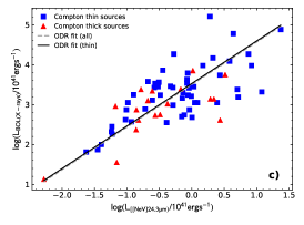
Figure 7: a: left AGN bolometric luminosity as a function of the [O IV] 25.89 $\mu$m  line luminosity. The blue squares indicate the Compton-thin AGN, while Compton-thick objects are denoted by red triangles. The solid lines represent the linear regression fit with all objects, while the dotted line the fit with only Compton-thin objects. b: center AGN bolometric luminosity as a function of the [NeV] 14.32 $\mu$m  line luminosity. c: right AGN bolometric luminosity as a function of the [NeV] 24.32 $\mu$m  line luminosity.

3.3 The X-ray correlation with other AGN strength indicators

In order to complete the picture of the observables correlated with the strength of an active nucleus in a galaxy, we have used the optical spectra of the 12$\mu$m AGN sample published in Malkan et al. (2017) to include the [OIII]$\lambda$5007Å line, and the observations of the 12$\mu$m nuclear flux given in Asmus et al. (2015). These two fluxes are in Table LABEL:tab:sample2, in columns (9) and (10), respectively.

Figures 22 and 23 in the Appendix show the correlations between fluxes and luminosities of the ($2$–$10)\,\rm{keV}$ X-ray band and of the ($14$–$195)\,\rm{keV}$ X-ray band fluxes and luminosities, respectively, with the [OIII]$\lambda$5007Å line flux and luminosity (panels (a) and (b), respectively). As can be seen from these figures and quantified in Table 2, the flux correlation between the [OIII]$\lambda$5007Å line and the ($2$–$10)\,\rm{keV}$ X-ray band is quite strong (P_null $\sim$ 10^-10), while the one with the ($14$–$195)\,\rm{keV}$ X-ray band is very weak (being P_null $\sim$ 10^-2) (see Fig.23(a)). This is partly due to the scarcity of the number of AGN that have 14-195keV data together with [OIII]$\lambda$5007Å line fluxes. Additionally the extremely hard X-ray band may present an intrinsically larger scatter due to a more uncertain proportionality to the intrinsic strength of the AGN, compared to the 2-10keV X-ray band (see, e.g. fig. 13 in Ricci et al., 2017a). The Luminosity correlations, as already discussed in section 3.1, are always strong, with probabilities P_null $\sim$ 10^-10 or even lower. The normalization of the [OIII] correlation with corrected ($2$–$10)\,\rm{keV}$ X-ray luminosity is very similar to that found recently by Saade et al. (2022). However, they identified a few Seyfert 2 galaxies fall well below the correlation perhaps because their hard X-ray emission has turned off for the last several decades.

Figures 24 and 25 in the Appendix show the correlations between fluxes and luminosities of the ($2$–$10)\,\rm{keV}$ X-ray band and of the ($14$–$195)\,\rm{keV}$ X-ray band, respectively, with the nuclear flux and luminosity measured at 12$\mu$m. The correlations between the ($2$–$10)\,\rm{keV}$ X-ray band flux and the 12$\mu$m nuclear flux is relatively strong (P_null $\sim$ 10^-4 for the whole AGN sample and P_null $\sim$ 10^-3 for the Compton- thin AGN), while at higher X-ray energies, the correlation becomes weaker (P_null $\sim$ 10^-3 for the whole AGN sample and P_null $\sim$ 10^-2 for the Compton-thin AGN). This is again due to the small number of AGN that have both 14-195keV data and 12$\mu$m nuclear fluxes and to the intrinsic scatter of the 14-195keV emission.

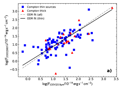
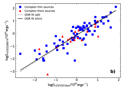
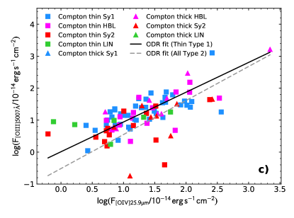
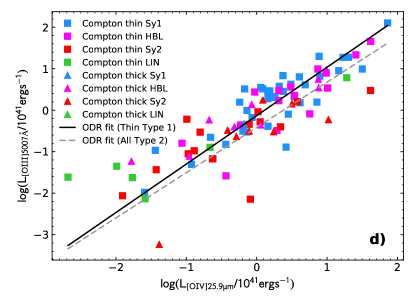
Figure 8: a: upper left [O III] 5007 Å  line flux as a function of the [O IV] 25.9$\mu$m line flux for all sources with reliable optical spectroscopic classification. Blue squares indicate Compton-thin objects, while red triangles Compton-thick. The solid line shows the fit for all Compton-thin AGN, while the broken line the fit for all objects. b: upper right [O III] 5007 Å  line luminosity vs. [O IV] line luminosity (both in logarithmic units of erg s^-1). The solid line shows the fit for all Compton thin AGN, while the broken line the fit for all objects. c: lower left Same as a:, but with the objects color coded: Seyfert types 1 (Sy1): blue; Hidden Broad Line Region Galaxies (HBL): magenta; Seyfert types 2 (Sy2): red; LINERS (LIN): green. The solid line shows the fit for all Compton thin Type 1 AGN, which include both Seyfert 1’s and HBL, while the broken line gives the bet fit for all the Type 2 objects, i.e. the pure Seyfert 2’s, both Compton thick and thin (see Table 2) b: lower right Same as b:, but with the objects color coded. All correlations are reported in Table 2

3.4 Flux and luminosity correlations between [O IV] 25.89 $\mu$m  and [O III] 5007 Å 

We show in Fig. 8(a) & (c) the correlation between the line fluxes of the [O III] 5007 Å  line and the [O IV] 25.89 $\mu$m  line, and in Fig. 8(b) & (d) the correlation between their luminosities, either considering all objects together and only Compton thin AGN and also considering all type 1’s together (including Seyfert 1’s and HBL) and all types 2. We do not find any significant difference in the correlation slopes (see Table 2) between either Compton thin or CT AGN and between type 1 and type 2 objects.

Meléndez et al. (2008) computed also the correlation between the [O III] 5007 Å  line luminosity and the [O IV] 25.89 $\mu$m  line luminosity in Seyfert galaxies and find a steeper correlation for Seyfert 2’s (B$\sim$1.8-2) compared to Seyfert 1’s (B$\sim$0.9). They also found that $L_{\rm[OIII]}$ correlates better with $L_{\rm 2-10keV}$ than $L_{\rm[OIV]}$ and suggest that this can be due to extinction affecting both [O iii] and $2$–$10\,\rm{keV}$, but not [O iv]. However, as already noticed, we better trust the flux correlations than the luminosity correlations: for our sample, the flux correlations are in agreement within the errors, with only a slightly higher Pearson coefficient in the flux correlation for the [O iii] ($\sim 0.68$) (see Table 2) when compared to that of the [O iv] ($\sim 0.58$) (see Table 1). The [O iv] luminosity correlation has a slightly higher slope coefficient ($0.88$) when compared to that of the [O iii] ($0.80$). We consider that the results of Meléndez et al. (2008) are not valid in general for the classes of AGN considered, because their smaller sample (40 galaxies only) might be biased toward high X-ray brightness (Rigby et al., 2009).

3.5 Bolometric luminosity: X-ray versus IR method

In Figure 9 we show the bolometric luminosity, as computed from the corrected ($2$–$10)\,\rm{keV}$ X-ray luminosity, using the bolometric correction of Lusso et al. (2012), as a function of the bolometric luminosity as computed from the [O IV] 25.89 $\mu$m  line luminosity with the calibration of Mordini et al. (2021) and the bolometric correction of Spinoglio et al. (1995). Fig. 9(a) shows the AGN divided in Compton-thin and Compton-thick, while Fig. 9(b) shows them divided in the various nuclear activity classes.

Table 2 gives the results of the ODR fit: it appears that the correlation is very strong, having one of the highest values of the Pearson coefficient ($\rho\sim$ 0.83, even if some caution has to be taken because these are luminosities). However the relation is not linear, with a slope of $B=1.4\pm 0.1$, meaning that the X-ray estimate of the bolometric luminosity is rising faster at higher luminosities with respect to the IR estimate. This may be ascribed to differences in the large bolometric corrections involved in both cases, typically of a factor of $\sim 10$, which include non-linear dependencies between the X-ray or mid-IR line fluxes and the total luminosities derived from them. For instance, Duras et al. (2020) show in their Fig. 6 the large discrepancies that exist among different X-ray bolometric corrections in the 2-10 keV band (Marconi et al., 2004). In Mordini et al. (2021), fig. 9b, we show that the luminosity estimates provided by the IR bolometric correction used in this work are closer to those based on the X-ray bolometric correction from Lusso et al. (2012) than those obtained using the X-ray correction in Marconi et al. (2004).

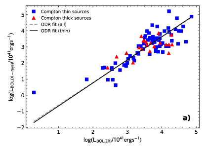
Figure 9: a: left Bolometric luminosity as derived from the 2-10keV X-ray luminosity using the Lusso et al. (2012) bolometric correction, as a function of the bolometric luminosity, as derived from the [OIV]26$\mu$m line luminosity and the bolometric correction of Spinoglio et al. (1995) according to the formula from Mordini et al. (2021). The luminosities are expressed in logarithmic units of 10⁴¹ erg s^-1. b: right Same as a, but with the objects color coded.

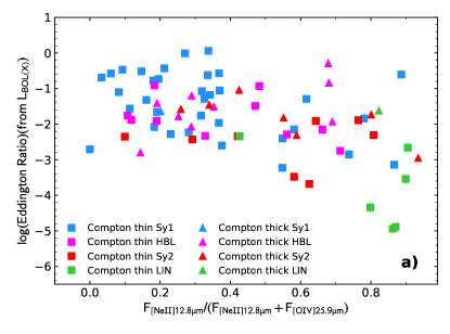
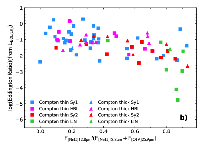
Figure 10: a: left Luminosity-Excitation diagram (LED) (Fernández-Ontiveros & Muñoz-Darias, 2021) showing the Eddington ratio (in logarithmic form) as a function of the [NeII]/[NeII]+[OIV] line ratio, which measures the accretion disk dominance in an AGN, following the results of Fernández-Ontiveros & Muñoz-Darias (2021). The Eddington ratio has been computed using the bolometric luminosity as derived from the X-ray 2-10keV luminosity. b: right Same as a, but with the the bolometric luminosity as derived from the [O IV] 25.89 $\mu$m  line and the bolometric correction of Spinoglio et al. (1995), using the formula from Mordini et al. (2021).

3.6 Accretion properties versus AGN types

3.6.1 Luminosity-Excitation Diagram

Fernández-Ontiveros & Muñoz-Darias (2021) presented the luminosity-excitation diagram (LED) using the mid-IR fine structure lines of [O IV] 25.9$\mu$m and [Ne II] 12.81 $\mu$m in the attempt to quantify the dominance of the accretion disk in various types of AGN, as a function of the Eddington ratio. The composite line ratio of [NeII]12.8$\mu$m/([O IV]25.9$\mu$m + [NeII]12.8$\mu$m), that we define as the “ionizing continuum softness” (hereafter called simply softness), is a good measure of the slope of the Lyman continuum due to the difference between the ionization potential of O³⁺ ($55\,\rm{eV}$) and Ne⁺ ($22\,\rm{eV}$). The accretion disk contribution in the extreme UV boosts significantly the [O IV] 25.89 $\mu$m  line intensity, which becomes very faint when the accretion disk cools or it is truncated (see fig. 3 of Fernández-Ontiveros & Muñoz-Darias 2021). As a consequence, the Lyman hardness is inversely proportional to the dominance of the accretion disk in AGN, being the softness:

$${\rm[NeII]/([OIV]+[NeII])~{}{\sim}~{}1-(L_{disk}/L_{total})}$$

The LED diagram in Fig. 10 shows the Eddington ratio as a function of the softness for our sample of AGN. The Eddington ratio is measured using the bolometric luminosity estimated from both the ($2$–$10)\,\rm{keV}$ X-ray luminosity (see Section 3.5; Fig. 10a) and from the mid-IR [OIV] fine structure line (Fig. 10b). This is divided by the estimated black hole mass, taken from the compilation in Fernández-Ontiveros & Muñoz-Darias (2021). One can see from this figure that using the X-ray determination of the bolometric luminosity has the effect of increasing the dispersion of the points in Eddington ratio, while the IR determination of the bolometric luminosity provides a better defined relation between the two axes, minimizing the spread in the Eddington ratio axis. On the other hand, IR-based luminosities tend to show slightly higher Eddington ratios, which can be caused by a small difference between the X-rays and the IR bolometric corrections.

At low values of the Eddington ratio (log $\lambda_{\rm Edd}<-3.0$), almost only LINERs are present, and these lie at very high values of the softness, i.e. at very low excitation as traced by the nebular gas, as it is indeed expected (Fernández-Ontiveros & Muñoz-Darias, 2021). On the other hand, most Seyfert 1 nuclei lie at low values of the softness (high gas excitation), due to the contribution of the accretion disk to the extreme UV continuum in these sources. Seyfert nuclei on the upper-right side of Fig. 10 are compatible with a cooler or a truncated accretion disk, which does not have enough UV photons to significantly boost the [O IV] 25.89 $\mu$m  emission line. Possible contamination in the [Ne II] 12.81 $\mu$m  line, due to strong star formation activity, could in principle shift the nuclei to the right side of this diagram, however most of the objects in our sample are AGN dominated sources. In order to quantify this statement, 57 objects – randomly selected, for which high-resolution Spitzer IRS spectra have been published – out of 117, i.e. $\sim 50\%$ of our sample, have an AGN fraction computed (Tommasin et al., 2010) and the average fraction is (85$\pm$15%), and therefore a negligible contribution from star formation to this line is expected.

Table 3 gives the statistics of the various AGN populations in terms of softness and Eddington ratio ($\lambda_{\rm Edd}$). Type 1 AGN, i.e. Seyfert type 1 and Hidden Broad Line Region galaxies (HBL) together, show on average higher Eddington ratios (log($\overline{\lambda_{\rm Edd}}$)=-1.2$\pm$1.0) and lower softness (${\rm[NeII]/([OIV]+[NeII])}=0.36{\pm}0.24$), while Seyfert type 2 galaxies show lower Eddington ratios (log($\overline{\lambda_{\rm Edd}}$)=-2.0$\pm$0.7) and intermediate softness (${\rm[NeII]/([OIV]+[NeII])}=0.6{\pm}0.3$) and Low Ionization Nuclear Emission Line galaxies (LINER) have even lower Eddington ratios (log($\overline{\lambda_{\rm Edd}}$) =-3.0$\pm$0.7) and higher softness (${\rm[NeII]/([OIV]+[NeII])}=0.8{\pm}0.3$), defining a decreasing trend among the three populations of AGN.

Table 1: Correlation of X-ray fluxes and luminosities with IR fine-structure lines.

Considered variables	Subset	N	$\rho$      (Pnull)	A $\pm\ \sigma$A	B $\pm\ \sigma$B
(1)	(2)	(3)	(4)	(5)	(6)
F(2-10keV) vs. F([NeV] 14.32 $\mu$m)	all	83	0.40 (1.9$\times 10^{-4}$)	0.28 $\pm$ 0.16	1.19 $\pm$ 0.17
”                    ”                    ”	C-thin	63	0.37 (3.0 $\times 10^{-3}$)	-0.23 $\pm$ 0.30	1.86 $\pm$ 0.36
F(2-10keV) vs. F([NeV] 24.32 $\mu$m)	all	72	0.46 (4.2 $\times 10^{-5}$)	-0.14 $\pm$ 0.18	1.21 $\pm$ 0.18
”                    ”                    ”	C-thin	54	0.48 (2.7 $\times 10^{-4}$)	-0.27 $\pm$ 0.28	1.67 $\pm$ 0.29
F(2-10keV) vs. F([O IV] 25.89 $\mu$m)	all	94	0.55 (1.2 $\times 10^{-8}$)	-0.58 $\pm$ 0.21	1.31 $\pm$ 0.15
”                    ”                    ”	C-thin	73	0.58 (7.7 $\times 10^{-8}$)	-0.88 $\pm$ 0.26	1.54 $\pm$ 0.19
”                    ”                    ”	Type 1	57	0.52 (3.1 $\times 10^{-5}$)	-0.51 $\pm$ 0.27	1.28 $\pm$ 0.19
”                    ”                    ”	Type 2	18	0.63 (4.8 $\times 10^{-3}$)	-1.67 $\pm$ 0.72	2.03 $\pm$ 0.52
F(2-10keV) vs. F([Ne III] 15.55 $\mu$m)	all	100	0.47 (7.0 $\times 10^{-7}$)	-2.03 $\pm$ 0.47	2.78 $\pm$ 0.41
”                    ”                    ”	C-thin	79	0.47 (1.4 $\times 10^{-5}$)	-2.67 $\pm$ 0.66	3.45 $\pm$ 0.61
F(2-10keV) vs. F([Ne II] 12.81 $\mu$m)	all	98	0.15 (1.4 $\times 10^{-1}$)	—	—
”                    ”                    ”	C-thin	77	0.07 (5.3 $\times 10^{-1}$)	—	—
F(14-195keV) vs. F([NeV] 14.32 $\mu$m)	all	58	0.44 (4.8 $\times 10^{-4}$)	1.01 $\pm$ 0.13	0.74 $\pm$ 0.12
”                    ”                    ”	C-thin	51	0.40 (3.8 $\times 10^{-3}$)	0.80 $\pm$ 0.17	0.99 $\pm$ 0.18
F(14-195keV) vs. F([NeV] 24.32 $\mu$m)	all	52	0.42 (2.2 $\times 10^{-3}$)	0.92 $\pm$ 0.16	0.76 $\pm$ 0.14
”                    ”                    ”	C-thin	45	0.36 (1.5 $\times 10^{-2}$)	0.64 $\pm$ 0.23	1.03 $\pm$ 0.22
F(14-195keV) vs. F([O IV] 25.89 $\mu$m)	all	61	0.45 (2.3 $\times 10^{-4}$)	0.65 $\pm$ 0.18	0.69 $\pm$ 0.11
”                    ”                    ”	C-thin	53	0.42 (1.8 $\times 10^{-3}$)	0.45 $\pm$ 0.22	0.82 $\pm$ 0.15
”                    ”                    ”	Type 1	46	0.40 (6.1 $\times 10^{-3}$)	0.37 $\pm$ 0.26	0.87 $\pm$ 0.17
”                    ”                    ”	Type 2	9	0.58 (1.0 $\times 10^{-1}$)	0.54 $\pm$ 0.52	0.83 $\pm$ 0.33
F(14-195keV) vs. F([Ne III] 15.55 $\mu$m)	all	62	0.45 (2.5 $\times 10^{-4}$)	0.75 $\pm$ 0.16	0.75 $\pm$ 0.12
”                    ”                    ”	C-thin	54	0.41 (1.9 $\times 10^{-3}$)	0.50 $\pm$ 0.21	0.97 $\pm$ 0.17
F(14-195keV) vs. F([Ne II] 12.81 $\mu$m)	all	60	0.29 (2.5 $\times 10^{-2}$)	1.25 $\pm$ 0.14	0.44 $\pm$ 0.11
”                    ”                    ”	C-thin	52	0.22 (1.2 $\times 10^{-1}$)	1.05 $\pm$ 0.17	0.53 $\pm$ 0.14
L(2-10keV) vs. L([NeV] 14.32 $\mu$m)	all	83	0.74 (9.6 $\times 10^{-16}$)	2.42 $\pm$ 0.07	1.00 $\pm$ 0.09
”                    ”                    ”	C-thin	63	0.76 (7.1 $\times 10^{-13}$)	2.45 $\pm$ 0.08	1.01 $\pm$ 0.10
L(2-10keV) vs. L([NeV] 24.32 $\mu$m)	all	72	0.70 (8.4 $\times 10^{-12}$)	2.37 $\pm$ 0.08	1.15 $\pm$ 0.12
”                    ”                    ”	C-thin	54	0.72 (9.2 $\times 10^{-10}$)	2.38 $\pm$ 0.09	1.23 $\pm$ 0.14
L(2-10keV) vs. L([O IV] 25.89 $\mu$m)	all	95	0.86 (5.1 $\times 10^{-29}$)	1.76 $\pm$ 0.07	1.17 $\pm$ 0.07
”                    ”                    ”	C-thin	74	0.88 (4.0 $\times 10^{-25}$)	1.79 $\pm$ 0.07	1.17 $\pm$ 0.07
”                    ”                    ”	Type 1	57	0.78 (5.8 $\times 10^{-13}$)	1.82 $\pm$ 0.08	1.17 $\pm$ 0.11
”                    ”                    ”	Type 2	18	0.77 (2.0 $\times 10^{-4}$)	1.88 $\pm$ 0.22	1.49 $\pm$ 0.28
L(2-10keV) vs. L([Ne III] 15.55 $\mu$m)	all	101	0.77 (4.6 $\times 10^{-21}$)	1.98 $\pm$ 0.08	1.41 $\pm$ 0.10
”                    ”                    ”	C-thin	80	0.78 (8.4 $\times 10^{-18}$)	1.98 $\pm$ 0.10	1.47 $\pm$ 0.12
L(2-10keV) vs. L([Ne II] 12.81 $\mu$m)	all	99	0.61 (1.5 $\times 10^{-11}$)	1.94 $\pm$ 0.12	1.65 $\pm$ 0.17
”                    ”                    ”	C-thin	78	0.62 (1.8 $\times 10^{-9}$)	1.96 $\pm$ 0.15	1.81 $\pm$ 0.21
L(14-195keV) vs. L([NeV] 14.32 $\mu$m)	all	58	0.76 (3.2 $\times 10^{-12}$)	2.78 $\pm$ 0.08	1.04 $\pm$ 0.10
”                    ”                    ”	C-thin	51	0.80 (1.9 $\times 10^{-12}$)	2.80 $\pm$ 0.08	1.04 $\pm$ 0.10
L(14-195keV) vs. L([NeV] 24.32 $\mu$m)	all	52	0.70 (7.3 $\times 10^{-9}$)	2.70 $\pm$ 0.09	1.18 $\pm$ 0.14
”                    ”                    ”	C-thin	45	0.74 (7.8 $\times 10^{-9}$)	2.69 $\pm$ 0.09	1.18 $\pm$ 0.14
L(14-195keV) vs. L([O IV] 25.89 $\mu$m)	all	61	0.85 (3.6 $\times 10^{-18}$)	2.19 $\pm$ 0.07	1.02 $\pm$ 0.07
”                    ”                    ”	C-thin	53	0.87 (2.3 $\times 10^{-17}$)	2.18 $\pm$ 0.08	1.03 $\pm$ 0.08
”                    ”                    ”	Type 1	46	0.77 (3.3 $\times 10^{-10}$)	2.11 $\pm$ 0.10	1.19 $\pm$ 0.13
”                    ”                    ”	Type 2	9	0.82 (7.3 $\times 10^{-3}$)	2.26 $\pm$ 0.17	0.92 $\pm$ 0.22
L(14-195keV) vs. L([Ne III] 15.55 $\mu$m)	all	62	0.85 (2.2 $\times 10^{-18}$)	2.45 $\pm$ 0.07	1.15 $\pm$ 0.08
”                    ”                    ”	C-thin	54	0.85 (3.9 $\times 10^{-18}$)	2.47 $\pm$ 0.07	1.16 $\pm$ 0.03
L(14-195keV) vs. L([Ne II] 12.81 $\mu$m)	all	60	0.77 (5.2 $\times 10^{-13}$)	2.52 $\pm$ 0.09	1.26 $\pm$ 0.12
”                    ”                    ”	C-thin	52	0.81 (3.3 $\times 10^{-13}$)	2.58 $\pm$ 0.10	1.28 $\pm$ 0.12

• Notes. Fit results. The $2$–$10\,\rm{keV}$ band fluxes and luminosities are intrinsic, i.e. corrected for the source intrinsic absorption measured from the X-ray spectra. The columns give for each correlation: (1) variables; (2) Subset of the entire sample on which the fit was computed: “C-thin” indicates the Compton-thin Sy1 and Sy2 subset, “all” indicates the entire sample with HX data; (3) Number of sources considered in the statistical analysis; (4) Pearson correlation coefficient $\rho$ (1: completely correlated variables, 0: uncorrelated variables) with the relative null hypothesis (zero correlation) probability; (5) and (6): Parameters of the linear regression fit using the equation: ${\rm log(F_{y})=A+B\times log(F_{x})}$ or ${\rm log(L_{y})=A+B\times log(L_{x})}$.

Table 2: Other correlation among X-ray fluxes and luminosities with other AGN indicators, bolometric luminosities and [O III] 5007 Å  and [O IV] 25.89 $\mu$m  fluxes and luminosities and SFR versus BHAR.

Considered variables	Subset	N	$\rho$      (Pnull)	A $\pm\ \sigma$A	B $\pm\ \sigma$B
(1)	(2)	(3)	(4)	(5)	(6)
F(2-10keV) vs. F([O III] 5007 Å)	all	91	0.59 (5.4$\times 10^{-10}$)	-0.66 $\pm$ 0.21	1.49 $\pm$ 0.16
”                    ”                    ”	C-thin	73	0.68 (3.4$\times 10^{-11}$)	-0.91 $\pm$ 0.22	1.70 $\pm$ 0.18
F(2-10keV) vs. F(12$\mu$m nuclear)	all	60	0.46 (1.9$\times 10^{-4}$)	-2.19 $\pm$ 0.58	1.52 $\pm$ 0.25
”                    ”                    ”	C-thin	47	0.45 (1.4 $\times 10^{-3}$)	-3.34 $\pm$ 0.94	2.05 $\pm$ 0.42
F(14-195keV) vs. F([O III] 5007 Å)	all	59	0.28 (3.4 $\times 10^{-2}$)	1.16 $\pm$ 0.14	0.38 $\pm$ 0.10
”                    ”                    ”	C-thin	52	0.32 (2.2 $\times 10^{-2}$)	0.84 $\pm$ 0.18	0.60 $\pm$ 0.13
F(14-195keV) vs. F(12$\mu$m nuclear)	all	39	0.49 (1.7 $\times 10^{-3}$)	-0.15 $\pm$ 0.39	0.81 $\pm$ 0.16
”                    ”                    ”	C-thin	33	0.44 (1.0 $\times 10^{-2}$)	-0.60 $\pm$ 0.54	1.01 $\pm$ 0.22
L(2-10keV) vs. L([O III] 5007 Å)	all	92	0.76 (2.9$\times 10^{-18}$)	1.91 $\pm$ 0.08	1.10 $\pm$ 0.09
”                    ”                    ”	C-thin	74	0.80 (6.8 $\times 10^{-18}$)	1.86 $\pm$ 0.09	1.18 $\pm$ 0.09
L(2-10keV) vs. L(12$\mu$m nuclear)	all	61	0.85 (8.1$\times 10^{-18}$)	-0.42 $\pm$ 0.18	0.99 $\pm$ 0.07
”                    ”                    ”	C-thin	48	0.85 (1.2 $\times 10^{-14}$)	-0.48 $\pm$ 0.20	1.01 $\pm$ 0.08
L(14-195keV) vs. F([O III] 5007 Å)	all	59	0.70 (5.9 $\times 10^{-10}$)	2.36 $\pm$ 0.07	0.69 $\pm$ 0.08
”                    ”                    ”	C-thin	52	0.75 (1.7 $\times 10^{-10}$)	2.34 $\pm$ 0.07	0.82 $\pm$ 0.09
L(14-195keV) vs. F(12$\mu$m nuclear)	all	39	0.92 (1.7 $\times 10^{-16}$)	-0.03 $\pm$ 0.17	1.00 $\pm$ 0.07
”                    ”                    ”	C-thin	33	0.93 (3.0 $\times 10^{-15}$)	-0.01 $\pm$ 0.17	1.01 $\pm$ 0.07
LBOL(2-10keV) vs. L([O IV] 25.89 $\mu$m)	all	94	0.84 (1.0 $\times 10^{-25}$)	3.02 $\pm$ 0.06	0.88 $\pm$ 0.06
”                    ”                    ”	C-thin	73	0.86 (3.9 $\times 10^{-22}$)	3.06 $\pm$ 0.06	0.89 $\pm$ 0.06
LBOL(2-10keV) vs. L([NeV] 14.32 $\mu$m)	all	82	0.70 (1.6 $\times 10^{-13}$)	3.53 $\pm$ 0.07	0.90 $\pm$ 0.08
”                    ”                    ”	C-thin	62	0.74 (1.0 $\times 10^{-13}$)	3.59 $\pm$ 0.08	0.86$\pm$ 0.09
LBOL(2-10keV) vs. L([NeV] 24.32 $\mu$m)	all	71	0.72 (1.6 $\times 10^{-12}$)	3.50 $\pm$ 0.07	1.06 $\pm$ 0.10
”                    ”                    ”	C-thin	53	0.71 (3.5 $\times 10^{-9}$)	3.53 $\pm$ 0.08	1.07$\pm$ 0.12
LBOL(2-10keV) vs. LBOL(IR)	all	94	0.83 (6.6 $\times 10^{-25}$)	-2.02 $\pm$ 0.33	1.41 $\pm$ 0.09
”                    ”                    ”	C-thin	73	0.85 (1.4 $\times 10^{-21}$)	-2.11 $\pm$ 0.35	1.43$\pm$ 0.10
F([O III] 5007 Å) vs. F([O IV] 25.89 $\mu$m)	All.	94	0.64 (2.5 $\times 10^{-12}$)	-0.20 $\pm$ 0.14	1.04$\pm$ 0.10
”                    ”                    ”	C-thin	76	0.62 (2.3 $\times 10^{-9}$)	-0.05 $\pm$ 0.14	0.94$\pm$ 0.11
F([O III] 5007 Å) vs. F([O IV] 25.89 $\mu$m)	Type 1	55	0.67 (2.1 $\times 10^{-8}$)	0.01 $\pm$ 0.16	0.93$\pm$ 0.11
”                    ”                    ”	Type 2	22	0.43 (4.5 $\times 10^{-2}$)	-0.51 $\pm$ 0.40	1.06$\pm$ 0.30
L([O III] 5007 Å) vs. L([O IV] 25.89 $\mu$m)	All	94	0.85 (1.7 $\times 10^{-27}$)	-0.15 $\pm$ 0.05	1.07$\pm$ 0.06
”                    ”                    ”	C-thin	76	0.86 (8.6 $\times 10^{-24}$)	-0.12 $\pm$ 0.06	1.04$\pm$ 0.06
L([O III] 5007 Å) vs. L([O IV] 25.89 $\mu$m)	Type 1	55	0.86 (4.9 $\times 10^{-17}$)	-0.13 $\pm$ 0.06	1.17$\pm$ 0.09
”                    ”                    ”	Type 2	22	0.71 (2.3 $\times 10^{-4}$)	-0.41 $\pm$ 0.16	1.09$\pm$ 0.20
SFR(M⊙/yr) vs. BHAR(M⊙/yr) from [CII]158$\mu$m	All	58	0.77 (1.2 $\times 10^{-12}$)	1.39 $\pm$ 0.10	0.53$\pm$ 0.05
”                    ”                    ”	C-thin	45	0.80 (2.7 $\times 10^{-11}$)	1.26 $\pm$ 0.11	0.50$\pm$ 0.05
SFR(M⊙/yr) vs. BHAR(M⊙/yr) from [CII]158$\mu$m	Type 1	33	0.73 (1.6 $\times 10^{-6}$)	1.41 $\pm$ 0.14	0.70$\pm$ 0.10
”                    ”                    ”	Type 2	12	0.79 (2.2 $\times 10^{-3}$)	1.76 $\pm$ 0.28	0.66$\pm$ 0.14
SFR(M⊙/yr) vs. BHAR(M⊙/yr) from PAH11.3$\mu$m	All	89	0.62 (1.1 $\times 10^{-10}$)	1.05 $\pm$ 0.12	0.53$\pm$ 0.06
”                    ”                    ”	C-thin	70	0.60 (3.3 $\times 10^{-8}$)	0.95 $\pm$ 0.14	0.48$\pm$ 0.06
SFR(M⊙/yr) vs. BHAR(M⊙/yr) from PAH11.3$\mu$m	Type 1	46	0.50 (4.5 $\times 10^{-4}$)	1.31 $\pm$ 0.23	0.81$\pm$ 0.14
”                    ”                    ”	Type 2	23	0.64 (1.0 $\times 10^{-3}$)	1.57 $\pm$ 0.32	0.74$\pm$ 0.15
sSFR(M⊙/yr) vs. LBOL(IR) from PAH11.3$\mu$m	All	78	0.44 (6.7 $\times 10^{-5}$)	-3.30 $\pm$ 0.36	0.67$\pm$ 0.10
”                    ”                    ”	C-thin	60	0.42 (8.5 $\times 10^{-4}$)	-3.10 $\pm$ 0.39	0.59$\pm$ 0.11
sSFR(M⊙/yr) vs. LBOL(IR) ) from PAH11.3$\mu$m	Type 1	43	0.17 (2.8 $\times 10^{-1}$)	-4.70 $\pm$ 1.00	0.99$\pm$ 0.26
”                    ”                    ”	Type 2	20	0.46 (4.1 $\times 10^{-2}$)	-5.01 $\pm$ 1.22	1.21$\pm$ 0.35
L(2-10keV) vs. L([O IV] 25.89 $\mu$m)	$L_{12\mu m}<10^{44}ergs^{-1}$	42	0.83 (6.8 $\times 10^{-12}$)	1.83 $\pm$ 0.11	1.26 $\pm$ 0.12
”                    ”                    ”	$L_{12\mu m}>10^{44}ergs^{-1}$	15	0.63 (1.2 $\times 10^{-2}$)	1.58 $\pm$ 0.41	1.76 $\pm$ 0.49
”                    ”                    ”	$\log(\lambda_{\rm Edd})<-1.5$	47	0.85 (3.8 $\times 10^{-14}$)	1.78 $\pm$ 0.11	1.28 $\pm$ 0.11
”                    ”                    ”	$\log(\lambda_{\rm Edd})>-1.5$	47	0.70 (3.7 $\times 10^{-8}$)	1.70 $\pm$ 0.11	1.27 $\pm$ 0.16

• Notes. Fit results. The $2$–$10\,\rm{keV}$ band fluxes and luminosities are intrinsic, i.e. corrected for the source intrinsic absorption measured from the X-ray spectra. The columns give for each correlation: (1) variables; (2) Subset of the entire sample on which the fit was computed: “C-thin” indicates the Compton-thin Sy1 and Sy2 subset, “all” indicates the entire sample with HX data; (3) Number of sources considered in the statistical analysis; (4) Pearson correlation coefficient $\rho$ (1: completely correlated variables, 0: uncorrelated variables) with the relative null hypothesis (zero correlation) probability; (5) and (6): Parameters of the linear regression as in Table 1.

Table 3: Line Excitation Diagram (LED) statistics

LBOL	Type	N	$\overline{\rm Soft.}$	$\sigma$	$log(\overline{\lambda_{\rm Edd}})$	$\sigma$
(1)	(2)	(3)	(4)	(5)	(6)	(7)
X-rays	SY1	36	0.35	0.25	-1.50	0.94
IR	”	37	0.34	0.24	-1.10	0.71
X-rays	HBL	20	0.38	0.22	-1.27	2.02
IR	”	19	0.39	0.22	-0.97	0.57
X-rays	Type1	56	0.36	0.24	-1.41	1.42
IR	(Sy1+HBL)	56	0.36	0.24	-1.06	0.67
X-rays	SY2	17	0.60	0.27	-2.31	0.74
IR	”	17	0.57	0.23	-1.58	0.56
X-rays	LIN	8	0.82	0.17	-3.32	1.28
IR	”	8	0.79	0.15	-2.52	1.38

• Notes. Column (1) gives the method for the computation of the bolometric luminosity, from which the Eddington ratio has been computed; Col.(2) the AGN type, note that Type 1 refers to the sum of the Seyfert 1’s and the HBL’s; Col.(3) the number of objects; Col.(4) and (5) the mean value of the softness and its standard deviation ($\sigma$); Col.(6) and (7) the mean value of the Eddington Ratio ${\lambda_{\rm Edd}}$ and its standard deviation ($\sigma$).

3.6.2 Eddington ratio as a function of the bolometric luminosity

Figure 11 shows the Eddington ratio as a function of the bolometric luminosity as computed from the corrected ($2$–$10)\,\rm{keV}$ X-ray luminosity, using the bolometric correction of Lusso et al. (2012) (panel a) and the Eddington ratio as a function of the bolometric luminosity as computed from the [O IV]  line luminosity with the calibration of Mordini et al. (2021) and the bolometric correction of Spinoglio et al. (1995) (panel b). The lines crossing the diagrams are the loci of the constant black-hole masses at 10⁷, 10⁸ and 10⁹ M_⊙, and show that most AGN have masses of the order of 10⁸ M_⊙. The median black hole mass is 5$\times 10^{7}\,\rm{M_{\odot}}$, spanning the range $\sim 10^{7}$–$10^{9}\,\rm{M_{\odot}}$ (Fig. 11).

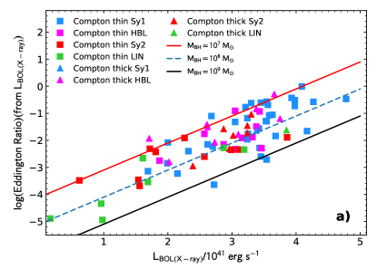
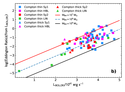
Figure 11: a: left The Eddington-ratio as a function of the bolometric luminosity as derived from the X-ray 2-10keV luminosity for the sub-sample of 12$\mu$m AGN with a BH mass estimate. Triangles indicate the Compton-Thick sources and the lines indicate three distinct BH-masses loci at 10⁷, 10⁸ and 10⁹ M_⊙. A clear separation between the HBL and the Sy2 populations is not observed either in the Eddington–ratio nor in the bolometric luminosity. b: right Same as a:, but with the the bolometric luminosity as derived from the IR [OIV]25.9 line and the bolometric correction of Spinoglio et al. (1995), using the formula from Mordini et al. (2021).

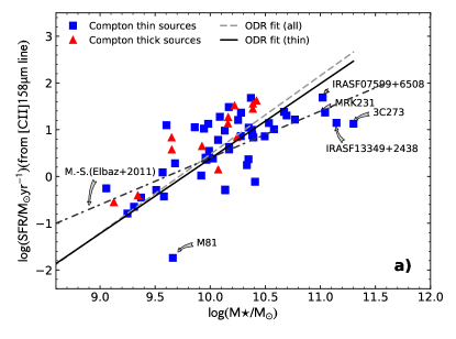
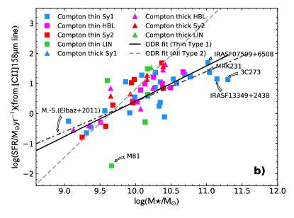
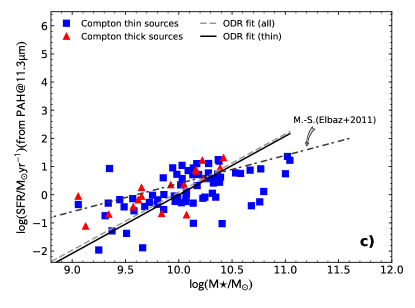
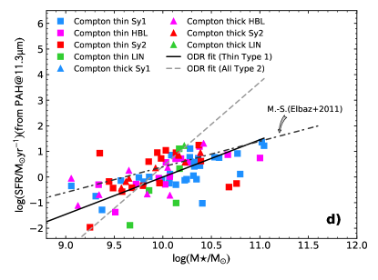
Figure 12: a: upper left The SFR, derived from the [CII]158$\mu$m fine structure line, as a function of the stellar mass of the galaxies. The galaxies are divided in Compton thick and Compton thin and the given fits are indistinguishable. The dot-dashed line represents the so called Main-Sequence for star forming galaxies (Elbaz et al., 2011). b: upper right Same as a:, but with the color coded galaxy types. c: lower left Same as a:, but with the SFR derived from the PAH 11.25$\mu$m emission band and the calibration from Xie & Ho (2019). d: lower right Same as c: but with the color coded galaxy types.

3.7 Star formation and black hole accretion in AGN

3.7.1 SFR versus stellar mass of the galaxy

To establish how much star formation is present per unit mass of a galaxy, the SFR vs galactic stellar mass diagram has been analyzed by Elbaz et al. (2011).

To measure the star formation rate in our AGN sample, we have used two different luminosities: the PAH 11.3$\mu$m emission feature and the [CII]158$\mu$m emission line. For the first feature we have used the calibration of Xie & Ho (2019) and the PAH 11.3$\mu$m fluxes of the 12$\mu$m sample from Wu et al. (2009). For the [CII]158$\mu$m line we have adopted the SFR formula given in Mordini et al. (2021), which has been derived for the Star forming galaxies, and therefore corrected for the scaling factor of the difference between SF galaxies and AGN (see Table D.1 in Mordini et al. (2021)). The [CII]158$\mu$m line data for our sample have been taken from Fernández-Ontiveros et al. (2016). We show in Fig.12a and b the diagram of the SFR, computed with the [CII] line luminosity, as a function of galaxy stellar mass and in Fig.12c and d the same diagram but with the SFR computed through the PAH 11.3$\mu$m emission feature.

The [Ne II] 12.81 $\mu$m  and [Ne III] 15.55 $\mu$m  SFR determination can, in principle, be applied only to star forming galaxies (Mordini et al., 2021) because these lines are also produced in the AGN NLR (especially the [Ne III] 15.55 $\mu$m), therefore a correction has to be applied, as e.g. given by Zhuang et al. (2019), which subtracts the AGN emission of these lines using the [NeV] 14.32 $\mu$m  line. As a comparison, we have included this determination in the Appendix (see Fig. 26).

Comparing the two methods to derive the SFR in galaxies, results in a slightly different normalization: the [CII]158$\mu$m line covers a range in SFR, from $\sim$0.1 $<$ SFR $\lesssim$ 60 M_⊙ yr^-1, while the PAH 11.3$\mu$m emission feature covers the range of $\sim$0.01 $<$ SFR $\lesssim$ 20 M_⊙ yr^-1. One can argue that in galaxies dominated from an AGN, the PAH emission might be suppressed to some extent by the highly energetic AGN radiation field, while the ionic fine structure lines, once corrected for the total IR luminosity contribution form the nucleus, can give a better estimate of the SFR. The dash-dotted line in all frames of Fig. 12 shows the so-called ”Main-Sequence” (M.S.) for star forming galaxies, we can see from all figures that most of the galaxies of our sample are below such a M.S. Moreover, while there is no difference between Compton-thin and Compton-thick objects, it appears that type 2 AGN have a steeper dependence of the SFR as a function of stellar mass and therefore have a higher SFR at a given galaxy mass. This result was already suggested by the analysis of mid-IR photometric data at 10$\mu$m from the ground, when compared to the IRAS 12$\mu$m data (Maiolino et al., 1995).

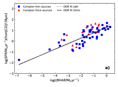
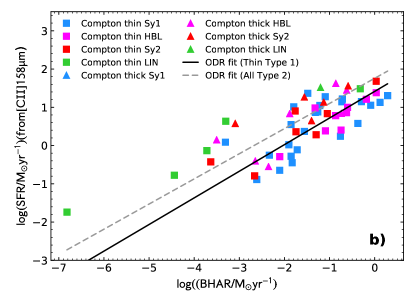
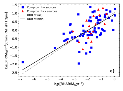
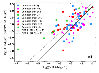
Figure 13: a: upper left Star Formation rate, as derived from the [CII]158$\mu$m line luminosity and the calibration of Mordini et al. (2021), as a function of the Black-hole accretion rate as derived from the [O IV] 25.89 $\mu$m line luminosity and the calibration from Mordini et al. (2021), adopting the bolometric correction of Lusso et al. (2012) for all objects and Compton thin only galaxies. Blue squares indicate Compton thin objects, while red triangles Compton thick. The solid line shows the fit for all Compton thin AGN, while the broken line the fit for all objects. b: upper right Same as in a but with the color coded objects and the fit of Compton thin type 1 galaxies and all type 2 galaxies. The value of the correlations is given in Table 2. c: lower left Same as in a, but with the Star Formation rate, as derived from the PAH11.3$\mu$m feature, as measured from low-resolution Spitzer data (Wu et al., 2009) and the calibration from Xie & Ho (2019). d: lower right Same as in c, but with the color coded objects and the fit of Compton thin type 1 galaxies and all type 2 galaxies.

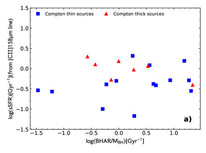
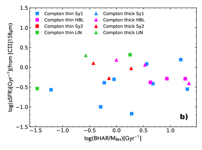
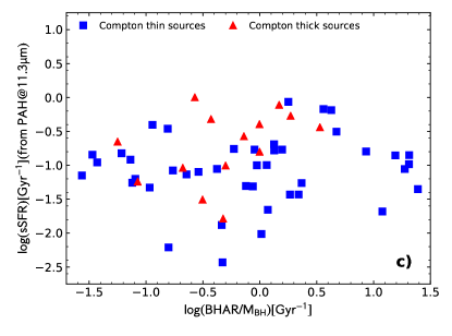
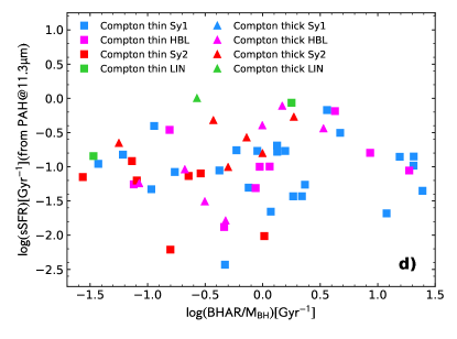
Figure 14: a: upper left Specific Star Formation rate, i.e. sSFR = SFR/M_⋆, as derived from the [CII]158$\mu$m luminosities and the calibration of Mordini et al. (2021) (see text), as a function of the specific Black-hole accretion rate, i.e sBHAR = BHAR/M_BH as derived from the [O IV] 25.89 $\mu$m line luminosity and the calibration from Mordini et al. (2021), adopting the bolometric correction of Lusso et al. (2012) for all objects and Compton thin only galaxies. Blue squares indicate Compton thin objects, while red triangles Compton thick. The solid line shows the fit for all Compton thin AGN, while the broken line the fit for all objects. b: upper right Same as in a but with the color coded objects and the fit of Compton thin type 1 galaxies and all type 2 galaxies. The value of the correlations is given in Table 2. c: lower left Same as in a, but with the Star Formation rate, as derived from the PAH11.3$\mu$m feature, as measured from low-resolution Spitzer data (Wu et al., 2009) and the calibration from Xie & Ho (2019). d: lower right Same as in c, but with the color coded objects and the fit of Compton thin type 1 galaxies and all type 2 galaxies.

3.7.2 Correlation between the SFR and the BHAR

We have derived the correlation between SFR and BHAR, as can be seen from Fig. 13 and in Table 2, measuring the BHAR with the [O IV] 25.89 $\mu$m  line and the calibration from Mordini et al. (2021), with the bolometric correction from Lusso et al. (2012) and computing the SFR in the two different ways described above (see section 3.7.1).

For the sub-sample of 58 AGN, for which the [CII]158$\mu$m line has been observed, using this SFR determination, we can derive the following formula (see Table 2):

$${\rm SFR(M_{\odot}/yr)=(24.5\pm 5.5)\cdot BHAR(M_{\odot}/yr)^{0.53}}$$ (4)

Using the PAH 11.3$\mu$m feature, for the sample of 89 galaxies for which we have measured this feature, we derive (see Table 2:

$${\rm SFR(M_{\odot}/yr)=(11.2\pm 3.2)\cdot BHAR(M_{\odot}/yr)^{0.53}}$$ (5)

Diamond-Stanic & Rieke (2012) used the same RSA Seyfert sample of 89 galaxies already discussed in Diamond-Stanic et al. (2009) to study the relationship between black-hole growth and star formation in Seyfert galaxies and found with the PAH11.3$\mu$m feature a steeper slope of $B\sim 0.8$, with a lower scaling factor of 7.6, but consistent within the errors.

As can be seen in Table 2, there is no significant difference between CT and Compton thin AGN. The small apparent difference between Type 1 and Type 2 AGN (see Table 2) is not statistically significant.

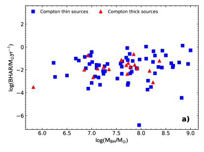
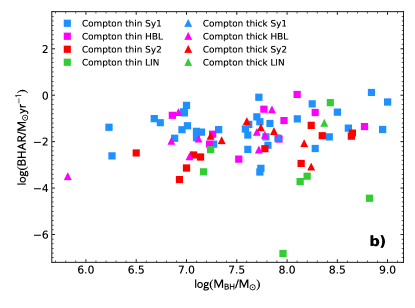
Figure 15: a: left Black hole accretion rate (BHAR), as derived from the [O IV] 25.89 $\mu$m line luminosity and the calibration from Mordini et al. (2021), adopting the bolometric correction of Lusso et al. (2012) as a function of the black-hole mass for all objects divided in Compton thin (blue squares) and Compton thick (red triangles). b: right Same as in a but with the color coded objects and the fit of Compton thin type 1 galaxies and all type 2 galaxies. Excluding the the low ionization emission line objects (LINER) an increasing trend of the BHAR ads a function of the BH mass is apparent in the data.

3.7.3 Correlation between specific SFR and “specific” BHAR

In Fig. 14, we show the specific SFR, i.e. the star formation rate divided by the stellar mass of the galaxy, sSFR = SFR / M${\star}$(M_⊙), as a function of what we name ”specific” BHAR, i.e. the black hole accretion rate divided by the black hole mass, sBHAR = BHAR / M_BH(M_⊙). Again, as in Section 3.7.1, we have determined the SFR using the two methods: in Fig. 14 a, b using the neon lines and in Fig. 14 c, d using the PAH. There is no correlation between the two quantities.

3.7.4 Black hole accretion rate as a function of the Black hole mass

In analogy with the SFR versus stellar mass diagram, we have plotted in Fig. 15 the BHAR as a function of the black hole mass. The lack of any correlation testifies that there is no dependence of the BHAR with the black hole mass.

4 Discussion

4.1 Correlations between NLR lines and X-rays

Bright forbidden emission lines from the NLR are usually adopted as unbiased orientation-independent tracers of the AGN bolometric power (Kauffmann et al., 2003; Heckman et al., 2004; Brinchmann et al., 2004). In particular, the correlation between the [O III] 5007 Å  line and the hard X-ray luminosity has been exploited in the past to derive bolometric corrections to the narrow emission line fluxes (e.g. LaMassa et al., 2009, 2010; Lamastra et al., 2009). Nevertheless, the optical narrow line fluxes can be affected by dust extinction, and thus a correction is required to derive reliable bolometric luminosities. Another caveat is the relatively low ionization potential of the bright narrow lines in the optical range. This is $35\,\rm{eV}$ in the case of [O III] 5007 Å, i.e. below the double ionization edge of helium ($54\,\rm{eV}$), meaning that non-negligible contamination from star formation activity is possible, especially in low-metallicity environments (e.g. Izotov et al., 2018). In this regard, the main advantages of using high-excitation lines in the mid-IR range is that these tracers are essentially unaffected by dust extinction and they probe unambiguously the accretion power in AGN (Genzel et al., 1998; Meléndez et al., 2008; Rigby et al., 2009).

In an X-ray selected sample of 40 galaxies, Meléndez et al. (2008) found a marginally stronger correlation between the 2-10 keV intrinsic luminosity and the [O III] 5007 Å  luminosity when compared to that obtained using the [O IV] 25.89 $\mu$m  line instead. This has been interpreted as uncorrected absorption affecting both the [O III] 5007 Å  and the 2-10 keV luminosities (Meléndez et al., 2008; Diamond-Stanic et al., 2009). In our 12$\mu$m-selected sample of 116 galaxies, we have analyzed both the flux and the luminosity correlations between the hard X-ray emission (2-10 keV and 14-195 keV) and the emission lines of [O IV] 25.89 $\mu$m  and the two [NeV] 14.32 $\mu$m  and [NeV] 24.32 $\mu$m  in the mid-IR, and the [O III] 5007 Å  optical line. In terms of flux, the [O IV] 25.89 $\mu$m  and the [O III] 5007 Å  lines show a similar correlation coefficient when compared with the 2-10 keV band for both the Compton-thin sub-sample and for the all the nuclei (Pearson coeff. $\rho\sim 0.6$; Tables 1 and 2). The correlations are weaker when the 14-195 keV band is considered ($\rho\sim 0.4$ for [O IV] 25.89 $\mu$m  and $\rho\sim 0.3$ for [O III] 5007 Å). These values are similar to those found by Berney et al. (2015) for the correlations between the optical lines and the X-ray fluxes in the AGN BAT sample. As expected, the distance factor boosts significantly all the correlations when the luminosities are considered ($\rho\gtrsim 0.7$). We conclude that no significant differences between the [O IV] 25.89 $\mu$m  and the [O III] 5007 Å  lines are found for our 12$\mu$m-selected sample. Thus, the selection criteria and the smaller number statistics in Meléndez et al. (2008) could explain the differences with our results.

When compared with the [O IV] 25.89 $\mu$m  line, the higher excitation lines of [NeV] 14.32 $\mu$m  show a weaker correlation with the 2-10 keV fluxes ($\rho\sim 0.4$), but comparable results for the 14-195 keV band. Overall, there is a correlation between the high excitation lines and the X-ray bands (Figs. 4, 5 and 6) with a large scatter in its flux version, which becomes significantly stronger only when the luminosities are considered.

The [Ne III] 15.55 $\mu$m  line requires a similar ionization potential as [O III] 5007 Å  ($41\,\rm{eV}$) and shows a weak correlation with both X-ray bands ($\rho\sim 0.45$; Fig. 20). In contrast, the lower excitation line of [Ne II] 12.81 $\mu$m  ($21\,\rm{eV}$) shows no correlation with either of the X-ray bands ($\rho\sim 0.2$ with p-null values of $\sim 10\%$; Fig. 21). Still, the corresponding luminosity correlations in both cases are strong ($\rho\gtrsim 0.6$), suggesting that the results obtained for the [Ne II] 12.81 $\mu$m  line are spurious.

We explore here if there is a possible dependence of the mid-IR high ionization lines with the covering factor (CF), i.e. the fraction of the sky seen from the AGN that is blocked by obscuring material. This could in principle block part of the NLR clouds from the primary excitation and ionization originating in the central supermassive black hole, and introduce systematic differences between sources with different covering factors. This could affect the NLR line to X-ray correlation and therefore introduce additional uncertainties in our results.

This effect can be serious for the so-called elusive AGN, where the nuclear UV source is completely embedded and the ionizing photons cannot escape, which prevents the formation of a classical narrow-line region (Maiolino et al., 2003) and for buried AGN found in LINER ULIRGs without optical Seyfert signatures (Imanishi et al., 2006).

An attempt to measure the covering factors of the mid-IR NLR lines of our sample of AGN is beyond the scope of the present paper, however, we have used an indirect method to test this scenario. The CF should be mainly driven by the AGN luminosity, because the obscuring material surrounding the nucleus recedes at higher AGN luminosities. This is shown by e.g. Toba et al. (2014) on the dependence of the CF from the mid-IR AGN luminosity, and by Ricci et al. (2017b) on the dependence of the CF from the Eddington ratio. These two tests demonstrate statistically that, for our sample, the mid-IR NLR lines are not affected by variations in the covering factor and therefore the results of this study, that the mid-IR NLR lines are a good indicator of the AGN intrinsic luminosity, are indeed robust.

Toba et al. (2014), using the Wide-field Infrared Survey Explorer (WISE, Wright et al., 2010) MIR all-sky survey and complete optical spectroscopy of emission lines for $\sim$ 3000 AGN-dominated MIR sources, found that the CF decreased with increasing MIR luminosity. In their Fig. 28, they show that the CF can be as high as 0.6$<$CF$\lesssim$0.8 for luminosities $L_{22\mu m}\lesssim 10^{44}ergs^{-1}$ and decreases to 0.2$<$CF$\lesssim$0.4 at $L_{22\mu m}\gtrsim 10^{44}ergs^{-1}$, thus defining a turnover luminosity at $L_{22\mu m}=10^{44}ergs^{-1}$. Following the arguments above, we have plotted in Fig.16a the X-ray (2–10) keV intrinsic luminosity as a function of the [O IV] 25.9$\mu$m line luminosity dividing the AGN with the nuclear 12$\mu$m luminosity above and below the turnover luminosity of $L_{12\mu m}=10^{44}ergs^{-1}$. We have adopted the nuclear 12$\mu$m luminosity, instead of the 22$\mu$m WISE luminosity used in Toba et al. (2014), because the nuclear 12$\mu$m luminosity is not affected by the galaxy emission. The result between the two fits, of high and low luminosity AGN, does not show any significant difference (see the fit results in Table 2). This indicates that, for our sample of AGN, there is no apparent effect of the covering factor affecting the mid-IR line luminosities. This is in line with the isotropic properties of the NLR lines found by Mulchaey et al. (1994).

Ricci et al. (2017b) confirmed the decrease in the covering factor of the circumnuclear material with increasing accretion rates, already found previously (Ueda et al., 2003; Maiolino et al., 2007; Treister et al., 2008; Burlon et al., 2011), using a systematic multi-wavelength survey of hard X-ray-selected black holes. Their result can be summarized by a relation between the covering factor of dusty gas and the Eddington ratio, inferred for both Compton-thick and Compton-thin AGN, that shows that the covering factor is significantly larger at $\log(\lambda_{\rm Edd})<-1.5$ ($\overline{CF}\sim 0.85$), and lower for $\log(\lambda_{\rm Edd})>-1.5$ ($\overline{CF}\sim 0.40$). We have therefore plotted in Fig.16b the X-ray (2–10) keV intrinsic luminosity as a function of the [O IV] 25.9$\mu$m line luminosity dividing the AGN by their Eddington ratio. The figure shows that there is no distinction between the objects with low and high Eddington ratio (see the fit results in Table 2).

In conclusion, we can affirm that for our sample of AGN, there is no apparent dependence of the NLR mid-IR lines from the covering factor of circumnuclear material around the nuclei.

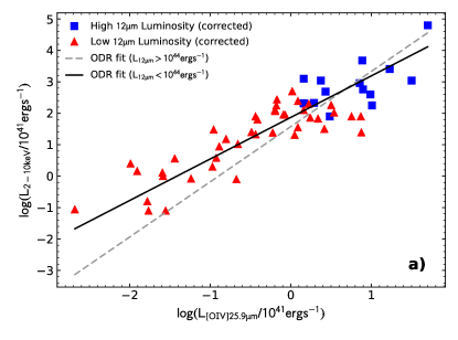
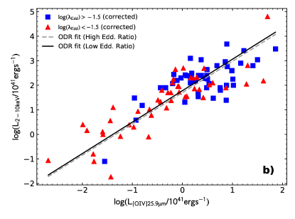
Figure 16: a: left X-ray (2–10) keV intrinsic luminosity as a function of the [O IV] 25.9$\mu$m line luminosity for all sources with a measure of the nuclear 12$\mu$m luminosity. The blue squares indicate the AGN with $L_{12\mu m}>10^{44}ergs^{-1}$, while red triangles show objects with $L_{12\mu m}<10^{44}ergs^{-1}$. The solid lines represent the linear regression fit with low luminosity objects, while the broken line shows the fit to the high luminosity objects. b: right Same as in a but with the AGN divided by their Eddington ratio: The blue squares indicate the AGN with $\log(\lambda_{\rm Edd})>-1.5$, while red triangles show objects with $\log(\lambda_{\rm Edd})<-1.5$.

4.2 Line to X-ray flux ratios in Seyferts 1 and 2

Meléndez et al. (2008) also found that the observed hard X-rays/[O iv] ratio is systematically lower in Seyfert 2 galaxies when compared to type 1 nuclei. This difference further increases for CT Seyfert 2’s. They interpret this result as absorption affecting the observed $2$–$10\,\rm{keV}$ spectra (corrected by Galactic N_H), which would even depress the observed luminosities in the hardest X-ray band ($14$–$195\,\rm{keV}$). In our Fig. 1(d) and Fig. 4(d), and in Table 1 we do not find any statistically significant difference, either comparing the whole sample of AGN with the Compton-thin objects only and dividing them in the two broad classes of type 1’s and type 2’s.

Diamond-Stanic et al. (2009) and Rigby et al. (2009) have tried to overcome the problems encountered by Meléndez et al. (2008) by selecting a complete sample of 89 optically selected Seyfert galaxies from the Revised Shapley-Ames sample (Maiolino & Rieke, 1995; Ho et al., 1997), containing 18 Seyfert 1’s and 71 Seyfert 2’s. Diamond-Stanic et al. (2009) have found that the [O IV] 25.89 $\mu$m  luminosity distributions of Seyfert 1’s and 2’s are indistinguishable and also that both Compton-thin and Compton-thick Seyfert 2’s are statistically indistinguishable from Seyfert 1’s. The same authors found that the correlation between the [O III] 5007 Å  luminosity and the [O IV] 25.89 $\mu$m  luminosity shows a significant difference between Seyfert 1’s and Seyfert 2’s with type 1’s having a [O IV] 25.89 $\mu$m/[O III] 5007 Å  ratio of order unity, while type 2’s have on average [O IV] 25.89 $\mu$m/[O III] 5007 Å$\sim 5$. To the contrary, we do not find any significant difference in this correlation for our sample, as can be seen either in the flux and in the luminosity correlations (see Sect. 3.4, Figs. 8 a–d) and Table 2).

Finally Diamond-Stanic et al. (2009) showed that the relation between the observed 2-10 keV X-ray luminosity and the [O IV] 25.89 $\mu$m  line luminosity of Seyfert 2’s (which include Compton thick objects) is significantly displaced compared to Seyfert 1’s. This is not a surprise because the observed 2-10 keV X-ray luminosities need to be corrected for absorption (see our Fig. 1(b,d) and Table 1). When this correction is applied, there is no statistical difference between Seyfert 1’s and 2’s.

Rigby et al. (2009) have used the same optically selected sample of Diamond-Stanic et al. (2009) to study the correlation between the [O IV] 25.89 $\mu$m  luminosity and the hard (10–200 keV) X-rays from Swift, INTEGRAL, and BeppoSAX. They found that Seyfert 2’s have systematically lower X-ray/[O IV]  luminosity ratios than Seyfert 1’s. In particular, for their sample, Seyfert 2’s have an average hard X-ray to [O IV]  ratio that is 3.1$\pm$0.8 times lower than Seyfert 1’s. their Compton-thin Seyfert 2’s show a decrement of 1.9 $\pm$0.5, and known Compton-thick Seyfert 2’s show a decrement of 5.0$\pm$2.7. To the contrary, with the complete mid-IR selected sample, we do not find any statistically significant difference among the various populations (all vs Compton-thin and AGN type 1’s vs type 2’s) either in flux or in luminosity (see Fig. 4 and Table 1). We ascribe their result to the heterogeneous hard X-ray coverage of their sample, being referred to different instruments with different observed energy ranges, which might cause significant systematic errors in the inferred X-ray luminosity of the considered AGN.

To establish the best isotropic indicators of intrinsic AGN luminosity, LaMassa et al. (2010) have identified five different proxies, namely the [O III] 5007 Å , the [O IV] 25.89 $\mu$m  line luminosities, the mid-IR, the radio and the hard X-ray (E $>$ 10 keV) continuum emission, using two complete samples of low-redshift Type 2 AGN: an optically selected [O III] 5007 Å  sample of 20 Seyfert 2’s galaxies and the original 12$\mu$m sample of 32 Seyfert 2’s (Spinoglio & Malkan, 1989). When they compared the Seyfert 2’s with the typical values of the Seyfert 1’s, they found that the mean ratio of the observed [O III] 5007 Å  flux to the [O IV] 25.89 $\mu$m  flux is lower in Seyfert 2’s than in Seyfert 1’s by a factor of 1.5–2. Analyzing the correlations in Table 2, shown in Figs. 8, as discussed already above and in Sect. 3.4, we are unable to confirm their result: the slopes of the correlations of Type 1’s and Type 2’s are well within the errors, and the intercepts have very large errors, therefore no statistically significant difference is apparent in our data.

LaMassa et al. (2010) have also found that the 14-195 keV hard X-ray flux (relative to the both [O III] 5007 Å  and [O IV]) is suppressed by about an order of magnitude in mid-IR selected Seyfert 2’s compared to Seyfert 1’s (consistent with Rigby et al. 2009). This is not the case for our larger complete 12$\mu$m selected sample of AGN, where the hard X-ray 14-195 keV X-ray data are more homogeneous and up-to-date, being collected mostly from the latest BAT survey (Oh et al., 2018), as can be seen in Fig. 4 and Table 1.

4.3 Accretion properties in a complete AGN sample

The luminosity-excitation diagram (LED; Fernández-Ontiveros & Muñoz-Darias 2021) for the AGN in the 12 $\mu$m sample, already introduced in Sect. 3.6.1, is shown in Fig. 10. It includes all galaxies of the sample with observations of the [O IV] 25.89 $\mu$m  and [Ne II] 12.81 $\mu$m  lines, a measure of the bolometric luminosity either from the X-ray emission or from the IR (see Section 3.5), and an estimate of the black hole mass (Section 3.6.1). In spite of the smaller number statistics, when compared to the heterogeneous sample analyzed in Fernández-Ontiveros & Muñoz-Darias (2021), especially among the LINER class, the 12 $\mu$m sample is complete and not biased toward type 1 or type 2 sources (Rush et al., 1993). Thus, it is a better sample to investigate intrinsic differences in the accretion properties of the various classes of AGN.

The clear distinction between type 1 and type 2 nuclei, which appears in the softness axis (see Sect. 3.6.1), with the majority of the Seyfert 1 population showing values of softness $<0.5$, caused by strong emission of the [O IV] 25.89 $\mu$m  line, is due to the intense UV radiation able to reach the high ionization potential of O³⁺ ($\sim 55\,\rm{eV}$), and is associated with the presence of a prominent accretion disk in these nuclei. This is also true for the hidden broad line Seyferts (HBL). Nevertheless, a certain fraction of the Seyfert 1 and HBL population (19% of Sy1 and 20-30% of HBL), depending on the method with which the bolometric luminosity is computed) is still found at softness values $>0.5$. The average value of the softness for type 1 AGN (Seyfert 1’s and HBL) is $\sim$0.36 (see table 3).

On the other hand, the Seyfert 2 population shows a wider distribution in excitation properties, with about half of the nuclei closer to the high excitation Seyfert 1’s and the other half at low excitation values, in agreement with the bimodal distribution found by Fernández-Ontiveros & Muñoz-Darias (2021) for the type 2 nuclei. The average value of the softness for type 2 nuclei is $\sim$0.6 (see Table 3).

In spite of the low statistics for the LINER in our sample, only 8 objects, the average value of the softness is $\sim$ 0.8, (see table 3), higher than any other AGN types, as expected for AGN lacking a significant contribution from the accretion disk in the UV range.

As already shown in Table 3, Type 1 nuclei (i.e. Seyfert 1’s and HBL galaxies) show on average higher Eddington ratios ($log(\overline{\lambda_{\rm Edd}})=-1.2\pm 0.2$) with respect to type 2 objects ($log(\overline{\lambda_{\rm Edd}})=-2.0\pm 0.3$), i.e. on average they appear to accrete more efficiently. As a matter of fact, very few Seyfert 2s are above $\sim 10\%$ Eddington, and most of the type 1s above this limit show prominent [O IV] 25.89 $\mu$m  emission and therefore high excitation. As expected, the lower Eddington luminosities observed correspond to LINER nuclei ($log(\overline{\lambda_{\rm Edd}})=-2.9\pm 0.4$). Two of the type 1 nuclei seem to be accreting at their Eddington limits in Fig. 10a, while Fig. 10b shows values slightly over Eddington. This is likely caused by an offset introduced by the different bolometric corrections applied to the X-ray and IR luminosities, although there is a good overall agreement between the two calibrations.

These results suggest that the accretion properties of type 1 and type 2 nuclei are intrinsically different. Most of the galaxies above $\sim 10\%$ Eddington are type 1s, which tend to show higher excitation values possibly due to the presence of a more dominant accretion disk in these nuclei. Half of the Seyfert 2s share similar excitation properties at lower luminosities, and could be consistent with the obscured Seyfert 1s in agreement with the unified model. The other half of the Seyfert 2 population and some of the type 1 nuclei show a relatively weak [O IV] 25.89 $\mu$m  emission, which could be explained by the lack of a prominent accretion disk in their ionizing continuum emission.

4.4 Host galaxy versus black hole properties

The result presented in Section 3.7.2 that a strong correlation (see the correlation parameters in Table 2) is found between the SFR and the BHAR should be analyzed carefully. This correlation does not necessarily mean that the two processes have a physical and causal link, but they may both depend on the fundamental physical quantity. In order to investigate the origin of this correlation we normalize both quantities by their related masses, the stellar mass of the galaxy for the SFR and the black hole mass for the BHAR, i.e. looking for a correlation between the specific SFR (sSFR) and the ratio of BHAR to the black hole mass. As shown in Section 3.7.3, no relation is found between the sSFR and the specific BHAR (Fig. 14), meaning that galaxies that are more efficient at forming stars do not necessarily feed their central black holes at a higher specific rate. Therefore, the correlation found between SFR and BHAR might be driven by the mass. That is, a massive galaxy would likely form more stars, it would host a heavier black hole at its center, which would be then more capable at producing energy through accretion processes. On the other hand, we cannot rule out the possibility that indeed a physical link exists among the two processes.

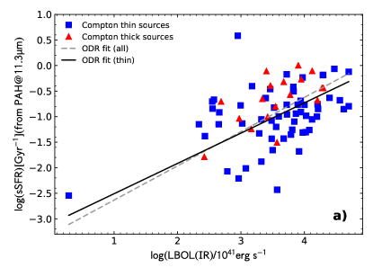
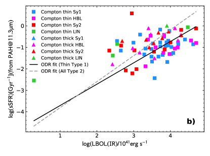
Figure 17: a: left Specific star formation rate (sSFR), as derived from the PAH11.3$\mu$m feature (Wu et al., 2009) and the calibration from Xie & Ho (2019), as a function of the bolometric luminosity, as derived from the IR, for all objects divided in Compton thin (blue squares) and Compton thick (red triangles). b: right Same as in a but with the color coded objects and the fit of Compton thin type 1 galaxies and all type 2 galaxies. Excluding the the low ionization emission line objects (LINER) an increasing trend of the BHAR ads a function of the BH mass is apparent in the data.

Our results presented in Section 3.7.2, showing a correlation between SFR and BHAR, can be compared with results of Zhuang & Ho (2020) who analyzed a large sample of optically selected type 1 and type 2 AGN and showed: i) a linear relation between AGN luminosity (accretion rate) and SFR and ii) that type-2 AGN, independent of stellar mass, Eddington ratio, redshift or molecular gas mass, exhibit intrinsically stronger star formation activity than type-1 AGNs. Both results are consistent with our findings. This is in apparent disagreement with the simplest AGN unified model in which there are no intrinsic differences between type 1 and type 2 Seyfert galaxies.

Moreover, our finding that normalizing to the mass makes the correlation disappear, is consistent with the results of Zhuang et al. (2021), who showed that the strong correlation between SFR and BHAR in their optically selected sample of 453 z$\sim$0.3 type 1 AGNs is driven by the mutual dependence of these parameters on the molecular gas mass. They also report that the SFR and BHAR are still weakly correlated after removing the dependence of star formation rate on molecular gas mass. However we do not see this effect using our – different – normalization.

Ward et al. (2022) have compared the results of simulations (TNG, EAGLE and SIMBA), also for the local Universe (epoch of redshift $z$ = 0), invoking AGN (negative) feedback to suppress star formation, with the observations searching signatures of AGN feedback by looking at trends between the bolometric luminosity and galaxy properties, or comparing AGN to non-AGN. The lack of negative trends between sSFR and AGN luminosity could indicate that AGN feedback may be ineffective. We have looked for correlations between the sSFR and the galaxy stellar mass, the AGN bolometric luminosity and the strength of the AGN as measured by the [O IV] 25.89 $\mu$m/[Ne II] 12.81 $\mu$m  line ratio (measuring the accretion disk dominance in AGN), but we did not find any negative tend. To the contrary, we find a positive correlation between the sSFR and the bolometric luminosity of the AGN, as can be seen in Fig. 17, that might indicate a positive AGN role in boosting the star formation. The results of the fit are given in Table 2.

4.5 What can be done by the JWST

The new James Webb Space Telescope (JWST; Gardner et al. 2006), launched on the 25th of December 2021, thanks to its mid-IR spectrometer MIRI (Rieke et al., 2015), can obtain spectra across the whole mid-IR range, for AGN and galaxies in the local Universe. This will provide local samples to study the co-existence of star formation and black hole accretion. Further, JWST will be able to observe the shorter wavelength high-ionization line of [NeV] 14.32 $\mu$m  up to a redshift of z$\sim$0.9, i.e. at the beginning of the so-called cosmic noon of galaxy evolution. The other high-ionization lines discussed in this paper, the [NeV] 24.32 $\mu$m  and the [O IV] 25.89 $\mu$m  lines, can be observed only at lower redshifts, namely at z$\lesssim$0.13, i.e. in the local Universe. However, other near-IR lines can be used to trace BHAR and SFR. The fine structure lines of [MgIV]4.49$\mu$m (IP = 80.1eV) and [ArVI]4.53$\mu$m (IP = 75eV) can be used as BHAR tracers for the 1 $<$ z $<$ 3 range, and the [NeVI]7.65$\mu$m line (IP = 126.2eV) as the best tracer for z $<$ 1.5 (Satyapal et al., 2021; Mordini et al., 2022). The [ArII]6.98$\mu$m (IP = 15.7eV) and [ArIII]8.99$\mu$m (IP = 27.6eV) lines can be used to measure the SFR at z $<$ 3 and z $<$ 2, respectively, while the stronger [NeII]12.8$\mu$m line is within the JWST-MIRI spectral range above z $<$ 1.2. At higher redshifts, the PAH features at 6.2 and 7.7$\mu$m can be observed at z $<$ 3 and z $<$ 2.7, respectively. We refer to the work of Mordini et al. (2022) for the assessment of these spectral lines and features, that can be detected by JWST-MIRI in galaxies and active galactic nuclei up to redshift z$\sim$3.

5 Summary

Unbiased tracers of the AGN power, detected even in dust-embedded regions, are essential to understand the co-evolution of supermassive black holes and their host galaxies. In this work we have demonstrated the potential of high-excitation emission lines in the mid-IR range to achieve this goal. Mid-IR transitions of ionic species with ionization potentials above the double ionization edge of helium ($>54\,\rm{eV}$) show a negligible contribution from stellar populations, and therefore are excellent isotropic tracers of the AGN contribution, unaffected by dust obscuration and temperature effects as opposed to the optical lines. This study is based on the 12$\mu$m AGN sample, a bolometric flux-limited sample unbiased by selection effects (e.g. dust obscuration, [O III] 5007 Å  luminosity), and the legacy of Spitzer/IRS for the spectroscopic observations of these galaxies. We compare the brightest high-excitation mid-IR lines ([O IV] 25.89 $\mu$m  and [NeV] 14.32 $\mu$m, [NeV] 24.32 $\mu$m) with the hard X-ray continuum and the [O III] 5007 Å  emission-line luminosities. Accretion power measurements derived from both X-ray continuum and the [O IV] 25.89 $\mu$m  line are used to investigate intrinsic differences among the various AGN types. Finally, we compare the main properties of the AGN host galaxies with those of the accreting supermassive black hole at their centers. The main conclusions of this study are:

• The 2-10keV X-ray fluxes and luminosities, only when corrected for absorption, give a robust measure of the AGN strength and these correlate with the high ionization mid-IR lines. The 14-195 keV hard X-ray fluxes also correlate with the mid-IR high ionization lines.

• The high ionization mid-IR fine structure lines ([NeV] 14.32 $\mu$m , [NeV] 24.32 $\mu$m  and [O IV] 25.89 $\mu$m) are a very powerful measure of the AGN strength and in particular the BHAR.

• Simple formulae are given to derive the AGN bolometric luminosities from the luminosity of one of the three high-ionization lines of [O IV] 25.89 $\mu$m, [NeV] 14.32 $\mu$m  and [NeV] 24.32 $\mu$m.

• The high-ionization mid-IR emission lines ([NeV] 14.32 $\mu$m, [NeV] 24.32 $\mu$m, [O IV] 25.89 $\mu$m) linearly correlate with other AGN bolometric indicators (compact nuclear $12\,\rm{\micron}$ emission, as well as [OIII] $\lambda$5007Å line emission), both in terms of flux and luminosity.

• No evidence of systematic differences in these correlations is found among the various Seyfert populations, including type 1 and type 2, and Compton-thick and -thin AGN.

• Differences are found between Seyfert type 1 and type 2 in the Eddington ratios and the excitation properties of the narrow line gas. Type 1 AGN, i.e. Seyfert type 1 and Hidden Broad Line Region galaxies (HBL) together, show on average higher Eddington ratios and stronger excitation, as traced by the [O IV]/[Ne II] line ratio, while Seyfert type 2 show lower Eddington ratios and lower excitation. Low Ionization Nuclear Emission Line galaxies (LINER) have even lower Eddington ratios and lower excitation, defining a decreasing trend among the three populations of AGN.

• In the mid-IR, the SFR in AGN can be measured by the PAH 11.3$\mu$m feature and in the far-IR with the fine structure line of [CII]158$\mu$m, once corrected for the offset between the luminosity of the AGN and the star forming galaxies.

• A positive correlation is found between the Black Hole Accretion Rate (BHAR) and the Star Formation Rate (SFR) (SFR$\propto$ $\sqrt{BHAR}$), measured through the [CII]158$\mu$m line and the PAH 11.3$\mu$m feature, but no correlation between the specific SFR (sSFR) and the specific BHAR, i.e. the BHAR/M_BH.

• The JWST will be able to measure these lines in many galaxies in the local Universe with the MIRI spectrograph, and assess the co-existence of star formation and black hole accretion. Moreover, the [NeV] 14.32 $\mu$m  line can be detected in AGN up to a redshift of z $\sim$0.9, allowing an accurate measure of the AGN bolometric luminosity, to be compared e.g., with the results of hard X-ray observations.

Appendix A Other figures with correlations

We present here the other correlations discussed in the main text. Fig.18 shows the (2-10)keV X-ray flux and luminosity as a function of the [Ne III] 15.55 $\mu$m  line flux and luminosity and Fig.19, the same for [Ne II] 12.81 $\mu$m. Fig.20 shows the (14-195)keV X-ray flux and luminosity as a function of the [Ne III] 15.55 $\mu$m  line flux and luminosity and Fig. 21 the same for the [Ne II] 12.81 $\mu$m  line.

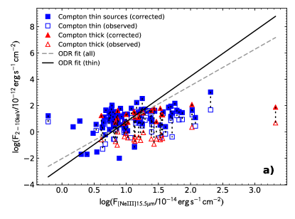
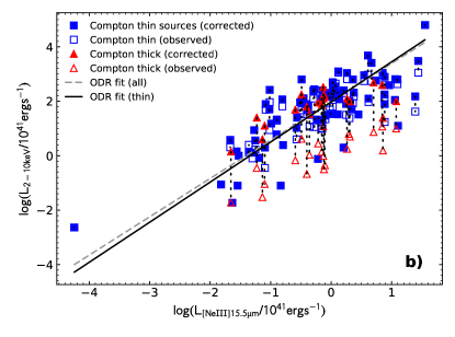
Figure 18: a: left X-ray (2–10) keV intrinsic flux as a function of the [Ne III] 15.55 $\mu$m line flux for all sources with reliable hard-X data and an optical spectroscopic classification. The blue squares indicate the Compton thin AGN, while Compton thick objects are denoted by red triangles. The solid lines represent the linear regression fit with all objects, while the dotted line the fit with only Compton thin objects. b: right X-ray (2-10) keV intrinsic luminosity vs. [Ne III] 15.55 $\mu$m line luminosity (both in logarithmic units of erg s^-1).

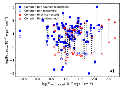
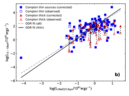
Figure 19: a: left X-ray (2–10) keV intrinsic flux as a function of the [Ne II] 12.81 $\mu$m  line flux for all sources with reliable hard-X data and an optical spectroscopic classification. The blue squares indicate the Compton thin AGN, while Compton thick objects are denoted by red triangles. The solid lines represent the linear regression fit with all objects, while the dotted line the fit with only Compton thin objects . b: right X-ray (2-10) keV intrinsic luminosity vs. [Ne II] 12.81 $\mu$m  line luminosity (both in logarithmic units of erg s^-1).

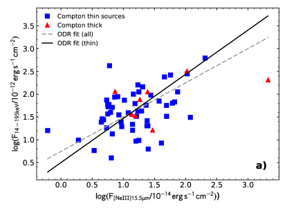
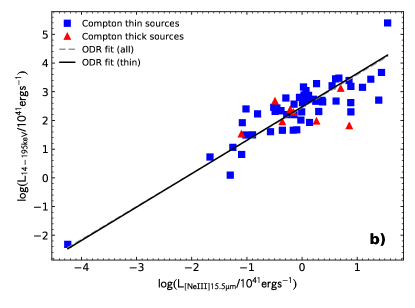
Figure 20: a: left X-ray (14-195) keV intrinsic flux as a function of the [Ne III] 15.55 $\mu$m  line flux for all sources with reliable hard-X data and an optical spectroscopic classification. The blue squares indicate the Compton thin AGN, while Compton thick objects are denoted by red triangles. The solid lines represent the linear regression fit with all objects, while the dotted line the fit with only Compton thin objects. b: right X-ray (14-195) keV intrinsic luminosity vs. [Ne III] 15.55 $\mu$m  line luminosity (both in logarithmic units of erg s^-1).

Fig.22 shows the (2-10)keV X-ray flux and luminosity as a function of the [OIII]$\lambda$5007$\AA$ line flux and luminosity and Fig. 23 the same for the (14-195)keV X-ray flux and luminosity. Fig.24 presents the (2-10)keV X-ray flux and luminosity as a function of the nuclear 12$\mu$m flux and luminosity from Asmus et al. (2014) and Fig. 25 the same for the (14-195)keV X-ray flux and luminosity.

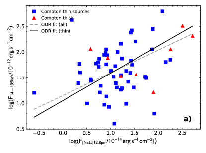
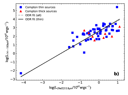
Figure 21: a: left X-ray (14-195) keV intrinsic flux as a function of the [Ne II] 12.81 $\mu$m  line flux for all sources with reliable hard-X data and an optical spectroscopic classification. The blue squares indicate the Compton thin AGN, while Compton thick objects are denoted by red triangles. The solid lines represent the linear regression fit with all objects, while the dotted line the fit with only Compton thin objects. b: right X-ray (14-195) keV intrinsic luminosity vs. [Ne II] 12.81 $\mu$m line luminosity (both in logarithmic units of erg s^-1).

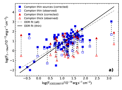
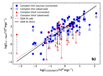
Figure 22: a: left X-ray (2-10) keV intrinsic flux as a function of the [O III] 5007 Å line flux for all sources with reliable hard-X data and an optical spectroscopic classification. The blue squares indicate the Compton thin AGN, while Compton thick objects are denoted by red triangles. The solid lines represent the linear regression fit with all objects, while the dotted line the fit with only Compton thin objects . b: right X-ray (2-10) keV intrinsic luminosity vs. [O III] 5007 Å  line luminosity (both in logarithmic units of erg s^-1).

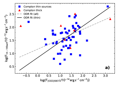
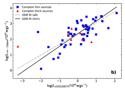
Figure 23: a: left X-ray (14-195) keV intrinsic flux as a function of the [O III] 5007 Å line flux for all sources with reliable hard-X data and an optical spectroscopic classification. The blue squares indicate the Compton thin AGN, while Compton thick objects are denoted by red triangles. The solid lines represent the linear regression fit with all objects, while the dotted line the fit with only Compton thin objects. b: right X-ray (14-195) keV intrinsic luminosity vs. [O III] 5007 Å  line luminosity (both in logarithmic units of erg s^-1).

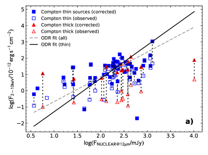
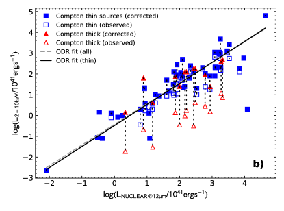
Figure 24: a: left X-ray (2-10) keV intrinsic flux as a function of the nuclear 12$\mu$m flux for all sources with reliable hard-X data and an optical spectroscopic classification. The blue squares indicate the Compton thin AGN, while Compton thick objects are denoted by red triangles. The solid lines represent the linear regression fit with all objects, while the dotted line the fit with only Compton thin objects. b: right X-ray (2-10) keV intrinsic luminosity vs. 12$\mu$m luminosity (both in logarithmic units of erg s^-1).

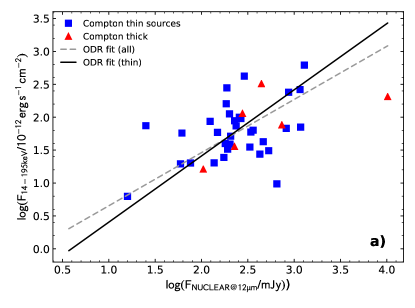
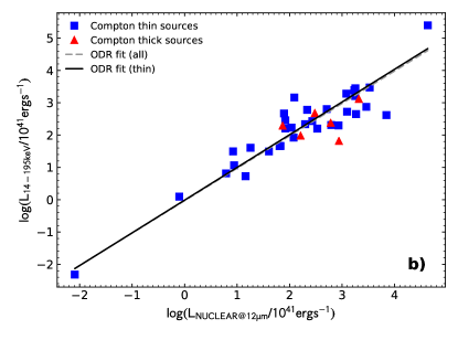
Figure 25: a: left X-ray (14-195) keV intrinsic flux as a function of the nuclear 12$\mu$m flux for all sources with reliable hard-X data and an optical spectroscopic classification. The blue squares indicate the Compton thin AGN, while Compton thick objects are denoted by red triangles. The solid lines represent the linear regression fit with all objects, while the dotted line the fit with only Compton thin objects. b: right X-ray (14-195) keV intrinsic luminosity vs. 12$\mu$m luminosity (both in logarithmic units of erg s^-1).

Fig.26 shows the SFR-Galaxy mass diagram from the SFR determination derived from the [Ne II] 12.81 $\mu$m  and [Ne III] 15.55 $\mu$m  lines. Finally Fig.27 shows the SFR, as derived from the neon lines, as a function of the BHAR.

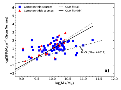
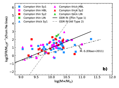
Figure 26: a: left The SFR, derived from the neon mid-IR fine structure lines, as a function of the stellar mass of the galaxies. The galaxies are divided in Compton thick and Compton thin and the given fits are indistinguishable. The dot-dashed line represents the so called Main-Sequence for star forming galaxies (Elbaz et al., 2011). b: right Same as a:, but with the color coded galaxy types.

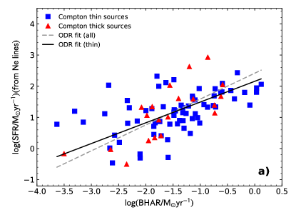
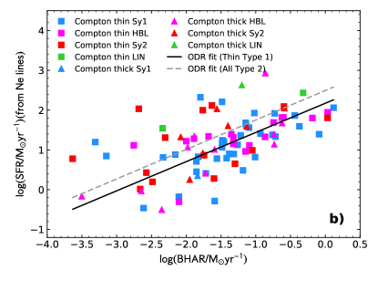
Figure 27: a: left Star Formation rate, as derived from the sum of the [Ne III] 15.55 $\mu$m  and [Ne II] 12.81 $\mu$m  luminosities and the calibration of Mordini et al. (2021) with the correction for AGN from Zhuang et al. (2019), as a function of the Black-hole accretion rate as derived from the [O IV] 25.89 $\mu$m line luminosity and the calibration from Mordini et al. (2021), adopting the bolometric correction of Lusso et al. (2012) for all objects and Compton thin only galaxies. Blue squares indicate Compton thin objects, while red triangles Compton thick. The solid line shows the fit for all Compton thin AGN, while the broken line the fit for all objects. b: right Same as in a but with the color coded objects and the fit of Compton thin type 1 galaxies and all type 2 galaxies. The value of the correlations is given in Table 2.

Appendix B Sample

We present here all the tables with the data of the sample.

Table 4: The AGN sample: coordinates, redshift, types

n.	Name	RA (J2000.0)	dec (J2000.0)	$z$	Type
	(1)	(2)	(3)	(4)	(5)
1	MRK0335	00:06:19.5	+20:12:10	0.0258	Sy1
2	NGC34=Mrk938=N17	00:11:06.5	-12:06:26	0.0196	Sy2
3	IRASF00198-7926	00:21:57.0	-79:10:14	0.0728	Sy2
4	ESO012-G021	00:40:47.8	-79:14:27	0.0300	Sy1
5	NGC0262=MRK348	00:48:47.1	+31:57:25	0.0150	HBL
6	Izw001=UGC00545	00:53:34.9	+12:41:36	0.0611	Sy1
7	IRASF00521-7054	00:53:56.2	-70:38:03	0.0689	HBL
8	ESO541-IG012	01:02:17.5	-19:40:09	0.0566	Sy2
9	NGC0424	01:11:27.5	-38:05:01	0.0118	HBL CT
10	NGC0526A	01:23:54.2	-35:03:56	0.0191	Sy1
11	NGC0513	01:24:26.8	+33:47:58	0.0195	HBL
12	IRASF01475-0740	01:50:02.7	-07:25:48	0.0177	HBL
13	MRK1034NED02	02:23:22.0	+32:11:50	0.0338	Sy1
14	ESO545-G013	02:24:40.2	-19:08:27	0.0337	Sy1
15	NGC0931=Mrk1040	02:28:14.5	+31:18:42	0.0167	Sy1
16	NGC1068	02:42:40.7	-00:00:48	0.0038	HBL CT
17	NGC1056	02:42:48.5	+28:34:29	0.0052	Sy2
18	NGC1097	02:46:19.1	-30:16:28	0.0042	LIN
19	NGC1125	02:51:40.4	-16:39:02	0.0109	HBL CT
20	NGC1144	02:55:12.2	-00:11:01	0.0288	Sy2
21	MCG-02-08-039	03:00:29.8	-11:24:59	0.0299	HBL
22	NGC1194	03:03:49.2	-01:06:12	0.0136	Sy1 CT
23	NGC1241	03:11:14.7	-08:55:20	0.0135	Sy2
24	NGC1320	03:24:48.7	-03:02:33	0.0089	Sy2
25	NGC1365	03:33:36.4	-36:08:25	0.0055	Sy1
26	NGC1386	03:36:45.4	-35:59:57	0.0029	HBL CT
27	IRASF03362-1642	03:38:34.5	-16:32:16	0.0369	Sy2
28	IRASF03450+0055	03:47:40.2	+01:05:14	0.0310	Sy1
29	NGC1566	04:20:00.6	-54:56:17	0.0050	Sy1
30	3C120	04:33:11.1	+05:21:16	0.0330	Sy1
31	MRK0618	04:36:22.2	-10:22:34	0.0356	Sy1
32	IRASF04385-0828	04:40:54.9	-08:22:22	0.0151	HBL
33	NGC1667	04:48:37.1	-06:19:12	0.0152	Sy2
34	ESO033-G002	04:55:59.6	-75:32:27	0.0181	Sy2
35	ESO362-G018	05:19:35.5	-32:39:30	0.0124	Sy1
36	IRASF05189-2524	05:21:01.4	-25:21:45	0.0426	HBL
37	ESO253-G003	05:25:18.3	-46:00:20	0.0425	Sy2
38	IRASF05563-3820	05:58:02.0	-38:20:05	0.0339	Sy1
39	MRK0006	06:52:12.2	+74:25:37	0.0188	Sy1
40	MRK0009	07:36:57.0	+58:46:13	0.0399	Sy1
41	MRK0079	07:42:32.8	+49:48:35	0.0222	Sy1
42	IRASF07599+6508	08:04:30.5	+64:59:53	0.1483	Sy1
43	NGC2639	08:43:38.0	+50:12:20	0.0111	Sy1
44	IRASF08572+3915	09:00:25.3	+39:03:54	0.0583	Sy2/LIN
45	MRK0704	09:18:26.0	+16:18:19	0.0292	Sy1
46	UGC05101	09:35:51.6	+61:21:11	0.0394	LIN CT
47	NGC2992	09:45:42.0	-14:19:35	0.0077	Sy1
48	MRK1239	09:52:19.1	-01:36:43	0.0199	Sy1
49	M81	09:55:33.2	+69:03:55	-0.00013	LIN
50	3C234	10:01:49.5	+28:47:09	0.1849	Sy1
51	NGC3079	10:01:57.8	+55:40:47	0.0037	Sy2 CT
52	NGC3227	10:23:30.6	+19:51:54	0.0039	Sy1
53	NGC3511	11:03:23.7	-23:05:11	0.0037	Sy1
54	NGC3516	11:06:47.5	+72:34:07	0.0088	Sy1
55	MCG+00-29-023	11:21:12.2	-02:59:03	0.0249	Sy2
56	NGC3660	11:23:32.2	-08:39:30	0.0123	Sy2
57	NGC3982	11:56:28.1	+55:07:31	0.0037	HBL
58	NGC4051	12:03:09.6	+44:31:53	0.0023	Sy1
59	UGC07064	12:04:43.3	+31:10:38	0.0250	HBL
60	NGC4151	12:10:32.6	+39:24:21	0.0033	Sy1
61	NGC4253=MRK766	12:18:26.5	+29:48:46	0.0129	Sy1
62	NGC4388	12:25:46.7	+12:39:41	0.0084	HBL
63	3C273	12:29:06.7	+02:03:09	0.1583	Sy1
64	NGC4501=M88	12:31:59.0	+14:25:10	0.0076	Sy2
65	NGC4579=M58	12:37:43.5	+11:49:05	0.0051	LIN
66	NGC4593	12:39:39.4	-05:20:39	0.0090	Sy1
67	NGC4594=M104	12:39:58.8	-11:37:28	0.0034	LIN
68	NGC4602	12:40:36.5	-05:07:55	0.0085	Sy1
69	TO1238-36=I3639	12:40:52.9	-36:45:22	0.0109	HBL CT
70	M-2-33-34=N4748	12:52:12.4	-13:24:54	0.0146	Sy1
71	MRK0231	12:56:14.2	+56:52:25	0.0422	Sy1
72	NGC4922	13:01:24.5	+29:18:30	0.0236	Sy2
73	NGC4941	13:04:13.1	-05:33:06	0.0037	Sy2
74	NGC4968	13:07:06.0	-23:40:43	0.0099	Sy2
75	NGC5005	13:10:56.2	+37:03:33	0.0032	LIN
76	NGC5033	13:13:27.5	+36:35:38	0.0029	Sy1
77	MCG-03-34-064	13:22:24.4	-16:43:43	0.0165	HBL
78	NGC5135	13:25:44.0	-29:50:02	0.0137	Sy2 CT
79	NGC5194=M51A	13:29:52.3	+47:11:54	0.0015	Sy2
80	MCG-06-30-015	13:35:53.7	-34:17:45	0.0077	Sy1
81	IRASF13349+2438	13:37:18.7	+24:23:03	0.1076	Sy1
82	NGC5256=Mrk266	13:38:17.8	+48:16:35	0.0279	Sy2
83	MRK0273	13:44:42.1	+55:53:13	0.0378	LIN
84	IC4329A	13:49:19.3	-30:18:34	0.0161	Sy1
85	NGC5347	13:53:17.8	+33:29:27	0.0078	HBL CT
86	MRK0463=UGC8850	13:56:02.9	+18:22:19	0.0504	HBL
87	NGC5506	14:13:14.8	-03:12:27	0.0062	Sy2
88	NGC5548	14:17:59.5	+25:08:12	0.0172	Sy1
89	MRK0817	14:36:22.1	+58:47:39	0.0315	Sy1
90	IRASF15091-2107	15:11:59.8	-21:19:02	0.0446	Sy1
91	NGC5929	15:26:06.1	+41:40:14	0.0083	HBL
92	NGC5953	15:34:32.3	+15:11:42	0.0066	Sy2
93	ARP220=UGC9913	15:34:57.3	+23:30:12	0.0181	Sy2
94	N5995=M-2-40-4	15:48:24.9	-13:45:28	0.0252	HBL
95	IRASF15480-0344	15:50:41.5	-03:53:18	0.0303	HBL
96	ESO141-G055	19:21:14.3	-58:40:13	0.0371	Sy1
97	IRASF19254-7245	19:31:22.5	-72:39:20	0.0617	HBL CT
98	NGC6810	19:43:34.1	-58:39:21	0.0068	LIN
99	NGC6860	20:08:46.1	-61:05:56	0.0149	Sy1
100	NGC6890	20:18:18.1	-44:48:23	0.0081	Sy2
101	MRK0509	20:44:09.7	-10:43:25	0.0344	Sy1
102	IC5063	20:52:02.0	-57:04:09	0.0113	HBL
103	MRK0897	21:07:45.8	+03:52:40	0.0263	Sy2
104	NGC7130	21:48:19.5	-34:57:09	0.0162	Sy2 CT
105	NGC7172	22:02:01.7	-31:52:18	0.0087	Sy2 CT
106	IRASF22017+0319	22:04:19.2	+03:33:50	0.0611	HBL
107	NGC7213	22:09:16.2	-47:10:00	0.0058	LIN
108	3C445	22:23:49.6	-02:06:12	0.0562	Sy1
109	NGC7314	22:35:46.0	-26:03:02	0.0048	HBL
110	MCG+03-58-007	22:49:36.9	-19:16:24	0.0315	HBL
111	NGC7469	23:03:15.6	+08:52:26	0.0163	Sy1
112	NGC7496	23:09:47.2	-43:25:40	0.0055	Sy2
113	NGC7582	23:18:23.5	-42:22:14	0.0053	Sy2 CT
114	NGC7590	23:18:55.0	-42:14:17	0.0053	Sy2
115	NGC7603	23:18:56.6	+00:14:38	0.0295	Sy1
116	NGC7674	23:27:56.7	+08:46:45	0.0289	HBL CT
117	CGCG381-051	23:48:41.3	+02:14:21	0.0307	Sy2

Table 4: continued.

Notes. The columns give for each AGN in the sample: (1) name; (2) AGN type: Sy1 = Seyfert type 1; Sy2 = Seyfert type 2; HBL = Hidden Broad Line Region AGN; LIN = LINER galaxy; (3) Hydrogen column density from the literature (see col. 11); (4) whether the galaxy is a Compton Thick object; (5) SWIFT name from Ricci et al. (2017a); or ${{\dagger}}$ from Cusumano et al. (2010) (6) intrinsic 2-10 keV X-ray flux; (7) observed 14-195 keV X-ray flux, from Oh et al. (2018); (8) logarithm of the 2-10 keV corrected X-ray luminosity; (9) logarithm of the 14-195 keV corrected X-ray luminosity; (10) Bolometric luminosity, as derived from the 2-10 keV X-ray luminosity, following Lusso et al. (2012); (11) references for the X-ray observations and hydrogen column densities, no X: means that no x-rays observations are available; 1: Ichikawa et al. (2019); 2: Ghosh & Soundararajaperumal (1992); 3: Ricci et al. (2017a); 4:Brightman & Nandra (2011); 5: Brightman & Nandra (2008); 6: Bassani et al. (1999); 7: Grupe et al. (2004); 8 :Akylas & Georgantopoulos (2009); 9 :Cardamone et al. (2007); 10: Risaliti et al. (2000); 11 :Risaliti et al. (1999); 12 :Guainazzi et al. (2005); 13 :Strickland (2007); 14 :González-Martín et al. (2009); 15 :Winter et al. (2008); 16: Lee et al. (2013); 17 :Lutz et al. (2004) ; 18: Deluit & Courvoisier (2003); 19: Cusumano et al. (2010); 20: Tan et al. (2012); 21: Iyomoto et al. (1996); 22: Polletta et al. (1996); 23: Iwasawa et al. (2011); 24: Liu et al. (2014); 25: Singh et al. (2011); 26: Ueda et al. (2001); 27: Bianchi et al. (2009); 28: Ueda et al. (2005); 29: Bianchi et al. (2008); 30: Teng et al. (2009); 31: Shu et al. (2010); 32: Bianchi et al. (2005); 33: Bi et al. (2020).

Table 5: X-ray properties of the AGN sample: & SWIFT ID., X-ray fluxes and luminosities.

n.	Name	Type	log(NH)	CT	SWIFT Name	F2-10keV	F14-195keV	log(L2-10keV)	log(L14-195keV)	log(LBOL(X))	refs.
			(cm-2)			($10^{-12}\rm{ergs^{-1}cm^{-2}}$)		($\rm{erg\,s^{-1}}$)
	(1)	(2)	(3)	(4)	(5)	(6)	(7)	(8)	(9)	(10)	(11)
1	MRK0335	Sy1	20.48		J0006.2+2012	16.69	15.97	43.42	43.40	44.56	1,3
2	NGC34=Mrk938=N17	Sy2	23.67		—	2.35	—	42.33	—	43.57	12,4
3	IRASF00198-7926	Sy2			—	—	21.8	—	44.44	—	18
4	ESO012-G021	Sy1	19.70		J0040.9-7915 ${{\dagger}}$	5.51	4.0	43.07	42.93	44.21	2,19
5	NGC0262=MRK348	HBL	23.12		J0048.8+3155	37.45	144.8	43.3	43.89	44.43	3,4
6	Izw001=UGC00545	Sy1	20.48		—	6.51	—	43.76	—	44.93	4,17
7	IRASF00521-7054	HBL			—	3.46	—	43.59	—	44.74	20
8	ESO541-IG012	Sy2			—	—	—	—	—	—	no X
9	NGC0424	HBL	24.33	Y	J0111.4-3808	28.4	21.51	42.95	42.85	44.10	3,4
10	NGC0526A	Sy1	22.30		J0123.8-3504	23.1	73.91	43.3	43.80	44.43	3,4,17
11	NGC0513	HBL	22.78		J0124.5+3350	5.57	24.47	42.7	43.34	43.87	1,3,4
12	IRASF01475-0740	HBL	24.30	Y	—	21.5	—	42.08	—	43.37	5,4
13	MRK1034NED02	Sy1			—	—	—	—	—	—	no X
14	ESO545-G013	Sy1			—	4.19	—	43.64	—	44.79	33
15	NGC0931=Mrk1040	Sy1	21.09		J0228.1+3118	29.19	62.22	43.28	43.61	44.42	1,3
16	NGC1068	HBL	$>$25.00	Y	J0242.6+0000	76.4	37.90	42.39	42.0	43.61	3,6
17	NGC1056	Sy2			—	—	—	—	—	—	no X
18	NGC1097	LIN	20.78		—	2.39	—	41.00	—	42.61	17,21
19	NGC1125	HBL	24.27	Y	J0251.6-1639	12.5	16.23	42.53	42.66	43.73	3
20	NGC1144	Sy2	23.76		J0255.2-0011	26.4	74.31	43.70	44.16	44.86	1,3
21	MCG-02-08-039	HBL	23.67		—	3.75	—	42.9	—	44.05	4
22	NGC1194	Sy1	24.33	Y	J0304.1-0108	42.5	36.22	43.25	43.20	44.38	3
23	NGC1241	Sy2			—	—	—	—	—	—	no X
24	NGC1320	Sy2	24.31	Y	—	29.3	—	42.7	—	43.87	4
25	NGC1365	Sy1	23.60		J0333.6-3607	44.15	63.52	42.5	42.66	43.70	3,4,17
26	NGC1386	HBL	20.66	Y	—	20.0	—	40.9	—	42.55	4
27	IRASF03362-1642	Sy2			—	—	—	—	—	—	no X
28	IRASF03450+0055	Sy1			—	—	—	—	—	—	no X
29	NGC1566	Sy1	20.00		J0420.0-5457	6.13	19.54	41.56	42.06	42.99	1,3
30	3C120	Sy1	21.45		J0433.0+0521	42.52	95.38	44.04	44.39	45.27	3
31	MRK0618	Sy1	20.95		J0436.3-1022	8.37	18.30	43.4	43.74	44.54	1,3,4
32	IRASF04385-0828	HBL			—	14.71	—	42.9	—	44.05	4,22
33	NGC1667	Sy2	$>$24.00	Y	—	11.53	—	42.8	—	43.96	6,4
34	ESO033-G002	Sy2	22.02		J0456.3-7532	2.63	24.49	42.31	43.2	43.55	3,6
35	ESO362-G018	Sy1	23.43		J0519.4-3240 ${{\dagger}}$	6.90	—	42.4	—	43.62	4,15
36	IRASF05189-2524	HBL	22.92		J0521.0-2522	4.14	9.71	43.25	43.62	44.38	1,3,4
37	ESO253-G003	Sy2			—	—	—	—	—	—	no X
38	IRASF05563-3820	Sy1	20.00		J0557.9-3822	46.26	27.45	44.1	43.87	45.35	1,3,4
39	MRK0006	Sy1	23.00		J0651.9+7426	15.04	56.70	43.1	43.68	44.24	3,4,17
40	MRK0009	Sy1	20.46		J0736.9+5846	6.8	9.84	43.40	43.57	44.54	1,3
41	MRK0079	Sy1	20.00		J0742.5+4948	54.07	42.72	43.8	43.70	44.98	1,3,4
42	IRASF07599+6508	Sy1			—	0.02	—	42.1	—	43.39	17
43	NGC2639	Sy1	23.62		—	2.06	—	41.78	—	43.15	6,4
44	IRASF08572+3915	Sy2/LIN			—	0.02	—	41.30	—	42.81	23
45	MRK0704	Sy1	20.00		J0918.5+1618	12.44	36.84	43.4	43.87	44.54	1,3,4
46	UGC05101	LIN	24.35	Y	J0935.9+6120	13.30	7.13	43.69	43.42	44.85	3,4
47	NGC2992	Sy1	21.72		J0945.6-1420	89.67	32.65	43.1	42.66	44.24	1,3,4
48	MRK1239	Sy1	23.48		—	21.87	—	43.312	—	44.45	7,24
49	M81	LIN	20.97		J0955.5+6907	10.5	20.26	38.36	38.68	41.17	3,4,17
50	3C234	Sy1	23.51		J1001.8+2848	3.73	5.82	44.48	44.67	45.88	1,3
51	NGC3079	Sy2	25.10	Y	J1001.7+5543	41.7	36.7	42.10	42.08	43.39	3,4
52	NGC3227	Sy1	22.81		J1023.5+1952	29.07	112.5	42.02	42.61	43.32	3,4,17
53	NGC3511	Sy1			—	—	—	—	—	—	no X
54	NGC3516	Sy1	20.60		J1106.5+7234	30.7	112.4	42.72	43.31	43.89	3,17
55	MCG+00-29-023	Sy2			—	—	—	—	—	—	no X
56	NGC3660	Sy2	20.48		—	2.43	—	41.94	—	43.26	5
57	NGC3982	HBL	23.63	Y	—	5.36	—	40.2	—	42.13	4,8
58	NGC4051	Sy1	20.00		J1203.0+4433	30.35	42.49	41.58	41.73	43.00	1,3,4
59	UGC07064	HBL	22.59		J1204.9+3105	2.4	13.48	42.54	43.30	43.74	1,3
60	NGC4151	Sy1	22.48		J1210.5+3924	1068.	618.9	43.44	43.20	44.58	3,4
61	NGC4253=MRK766	Sy1	21.90		J1218.5+2952	36.68	26.17	43.16	43.01	44.30	3,4
62	NGC4388	HBL	23.63		J1225.8+1240	47.54	278.9	42.9	43.67	44.05	3,4
63	3C273	Sy1	20.00		J1229.1+0202	106.3	421.6	45.8	46.40	—	3,4
64	NGC4501=M88	Sy2	$>$24.00		—	0.61	—	40.92	—	42.56	4,5
65	NGC4579=M58	LIN	22.38		J1237.7+1150 ${{\dagger}}$	3.91	—	41.11	—	42.69	4,17
66	NGC4593	Sy1	20.30		J1239.6-0519	61.26	88.30	43.07	43.23	44.21	3,4,17
67	NGC4594=M104	LIN	21.74		—	1.39	—	39.94	—	41.98	4,6
68	NGC4602	Sy1			—	—	—	—	—	—	no X
69	TOL1238-36=IC3639	HBL	24.2	Y	—	63.2	—	42.38	—	43.61	12
70	M-2-33-34=NGC4748	Sy1	20.00		J1252.3-1323	5.89	9.35	42.47	42.67	43.68	1,3
71	MRK0231	Sy1			—	0.79	—	42.52	—	43.72	4,25
72	NGC4922	Sy2			—	—	—	$<$37.64	—	—	no X, 33
73	NGC4941	Sy2	23.72		J1304.3-0532	6.16	20.16	41.30	41.81	42.81	3
74	NGC4968	Sy2	$>$24.00	Y	—	62.3	—	43.2	—	44.34	4,6
75	NGC5005	LIN	20.00		—	—	—	39.9	—	41.96	4,14
76	NGC5033	Sy1	22.46		J1313.6+3650B	6.47	6.26	41.11	41.10	42.69	3,17
77	MCG-03-34-064	HBL	23.80		J1322.2-1641	12.32	30.98	42.9	43.30	44.05	1,3,4
78	NGC5135	Sy2	$>$24.00	Y	—	42.8	—	43.26	—	44.39	6,26
79	NGC5194=M51A	Sy2	24.00		—	27.13	—	41.16	—	42.72	4,6,14
80	MCG-06-30-015	Sy1	20.85		J1335.8-3416	56.58	59.53	42.90	42.92	44.05	1,3,4
81	IRASF13349+2438	Sy1	21.66		—	2.36	—	43.81	—	44.99	16,27
82	NGC5256=Mrk266	Sy2	$>$25.00	Y	—	5.43	—	43.0	—	44.14	10,12
83	MRK0273	LIN	23.69		J1344.2+5551 ${{\dagger}}$	3.32	—	43.05	—	44.19	4,6
84	IC4329A	Sy1	21.62		J1349.3-3018	148.6	263.3	43.96	44.21	45.17	3,4,17
85	NGC5347	HBL	$>$24.00	Y	—	22.0	—	42.48	—	43.69	11,28
86	MRK0463=UGC8850	HBL	23.57		J1355.9+1822	2.52	8.48	43.18	43.71	44.32	1,3,17,28
87	NGC5506	Sy2	22.53		J1413.2-0312	74.28	239.4	42.83	43.34	43.99	3,4,17
88	NGC5548	Sy1	21.71		J1417.9+2507	35.04	86.47	43.39	43.78	44.53	3,4,17
89	MRK0817	Sy1	20.00		J1436.4+5846	13.6	28.77	43.49	43.83	44.63	1,3
90	IRASF15091-2107	Sy1	21.28		J1512.0-2119	16.86	32.67	43.9	44.19	45.09	1,3,4
91	NGC5929	HBL	23.44		—	1.50	—	41.39	—	42.87	9,25
92	NGC5953	Sy2			—	$<$0.005	—	$<$39.73	—	—	12
93	ARP220=UGC9913	Sy2			—	0.01	—	40.88	—	42.54	30
94	N5995=MCG-2-40-4	HBL	21.97		J1548.5-1344	14.9	35.21	43.33	43.72	44.46	1,3,28
95	IRASF15480-0344	HBL	$>$24.20	Y	—	4.60	—	43.0	—	44.14	4,12
96	ESO141-G055	Sy1	20.74		J1921.1-5842	33.64	58.77	44.04	44.28	45.27	3,17
97	IRASF19254-7245	HBL	$>$24.00	Y	—	35.1	—	42.8	—	43.96	4,17,26
98	NGC6810	LIN	22.00		—	0.08	—	39.9	—	41.96	4,13
99	NGC6860	Sy1	21.08		J2009.0-6103	25.6	51.52	43.11	43.43	44.25	1,3,15
100	NGC6890	Sy2	23.38		—	9.74	—	42.18	—	43.45	4,9,28
101	MRK0509	Sy1	20.00		J2044.2-1045	170.8	100.14	44.68	44.45	46.21	1,3,4,27
102	IC5063	HBL	23.56		J2052.0-5704	34.63	67.76	43.02	43.31	44.16	1,3
103	MRK0897	Sy2			—	—	—	—	—	—	no X
104	NGC7130	Sy2	24.00	Y	J2148.3-3454	6.10	17.41	42.55	43.03	43.75	3,14,26
105	NGC7172	Sy2	22.91		J2201.9-3152	50.89	160.02	42.96	43.46	44.11	1,3,4
106	IRASF22017+0319	HBL	22.83		J2204.7+0337	7.2	16.16	43.80	44.15	44.98	1,3
107	NGC7213	LIN			J2209.4-4711	62.92	39.04	42.7	42.49	43.87	3,4
108	3C445	Sy1	23.43		J2223.9-0207	34.37	39.82	44.41	44.47	45.78	1,3,4
109	NGC7314	HBL	22.08		J2235.9-2602	41.8	57.42	42.33	42.50	43.57	3,4,17
110	MCG+03-58-007	HBL	23.44		—	2.13	—	42.7	—	43.87	4
111	NGC7469	Sy1	20.53		J2303.3+0852	33.21	70.63	43.32	43.65	44.45	1,3,4
112	NGC7496	Sy2			—	—	—	—	—	—	no X
113	NGC7582	Sy2	24.33	Y	J2318.4-4223	120.	82.28	42.86	42.74	44.02	3,4
114	NGC7590	Sy2			—	0.03	—	39.27	—	41.62	26,31
115	NGC7603	Sy1	20.00		J2318.9+0013	22.04	52.96	43.65	44.04	44.68	1,3,25
116	NGC7674	HBL	$>$25.00	Y	—	20.	—	43.6	—	44.75	17,32
117	CGCG381-051	Sy2			—	—	—	—	—	—	no X

Table 5: continued.

Table 6: Observed and absorption corrected (2-10) keV fluxes and luminosities for Compton thick objects.

n.	Name	Type	log(NH)	FX(OBS)	FX(COR)	log(LX)(OBS)	log(LX)(COR)	(ref.)
			(cm-2)	($10^{-12}\,\rm{erg\,s^{-1}\,cm^{-2}}$)		($\rm{erg\,s^{-1}}$)
	(1)	(2)	(3)	(4)	(5)	(6)	(7)	(8)
9	NGC0424	HBL	24.33	0.9	28.4	41.45	42.95	1
12	IRASF01475-0740	HBL	24.30	0.82	21.5	40.66	42.08	2,5
16	NGC1068	HBL	$>$25	4.9	76.4	41.19	42.39	1
19	NGC1125	HBL	24.27	0.4	12.5	41.03	42.53	1
22	NGC1194	Sy1	24.33	1.0	42.5	41.62	43.25	1
24	NGC1320	Sy2	24.00	0.48	29.3	40.83	42.7	3,5
26	NGC1386	HBL	23.55	0.32	20.0	39.48	40.9	3,5
33	NGC1667	Sy2	$>$24	0.10	11.5	40.33	42.80	3,5
46	UGC05101	LIN	24.35	0.2	13.3	41.87	43.69	1
51	NGC3079	Sy2	25.10	0.3	41.7	39.96	42.10	1
57	NGC3982	HBL	23.63	0.19	5.36	39.28	40.2	3,4
69	TOL1238-36=I3639	HBL	24.2	0.08	63.2	40.50	42.38	2,3
74	NGC4968	Sy2	$>$24.	0.26	62.3	40.65	43.2	3,5
78	NGC5135	Sy2	$>$24.	0.23	42.8	40.99	43.26	3,6
82	NGC5256=Mrk266	Sy2	$>$25.	0.36	5.43	41.8	43.0	4
85	NGC5347	HBL	$>$24.	0.26	22.0	40.55	42.48	3,7
95	IRASF15480-0344	HBL	24.2	0.45	4.60	41.7	43.0	5
97	IRASF19254-7245	HBL	$>$24.	0.25	35.1	42.0	42.8	5
104	NGC7130	Sy2	$>$24.0	0.3	6.1	41.25	42.55	1
113	NGC7582	Sy2	24.33	2.3	120.	41.14	42.86	1
116	NGC7674	HBL	$>$25.	0.60	20.	42.07	43.6	5

• Notes. The columns give for each AGN in the sample: (1) name; (2) AGN type (see Table LABEL:tab:sample1) ; (3) logarithm of Hydrogen intrinsic absorption column density (see Table LABEL:tab:sample1); (4) observed F_2-10keV flux; (5) absorption corrected F_2-10keV flux; (6) observed L_2-10keV; (7) absorption corrected L_2-10keV; (8) reference: 1: observed and corrected 2-10 keV fluxes and luminosities from extrapolated 14-150keV data by Ricci et al. (2017a); 2: Guainazzi et al. (2005); 3: observed 2-10 keV fluxes and luminosities from LaMassa et al. (2011); 4: Ueda et al. (2005); 5: Brightman & Nandra (2011); 6: Yamada et al. (2020); 7: Levenson et al. (2006).

Notes. The columns give for each AGN in the sample: (1) name; (2) redshift; (3) AGN type (see Table LABEL:tab:sample1) ; (4) $\rm[NeII]12.8\mu m$ flux; (5) $\rm[NeIII]15.5\mu m$ flux; (6) $\rm[NeV]14.3\mu m$ flux; (7) $\rm[NeV]24.3\mu m$ flux; (8) $\rm[OIV]26\mu m$ flux; (9) $\rm PAH\,11.3\mu m$ flux from Wu et al. (2009), where available, otherwise from Tommasin et al. (2008, 2010); (10) $\rm[CII]158\mu m$ flux from Fernández-Ontiveros et al. (2016) (11) $\rm[OIII]\lambda 5007$ flux from Malkan et al. (2017), ^† from LaMassa et al. (2010), ^‡ from Koss et al. (2017) ; (11) nuclear 12${\mu}m$ flux from Asmus et al. (2014). The IR line fluxes have been taken from Tommasin et al. (2008, 2010). Note that $\rm[NeV]1$ refers to the $\rm[NeV]14.3\mu m$ line, $\rm[NeV]2$ refers to the $\rm[NeV]24.3\mu m$ line. Other notes: ¹ data fom Efstathiou et al. (2014)

Table 7: Observed properties of the local galaxy sample: AGN types, IR lines and continuum fluxes.

				Line and continuum fluxes
n.	Name	$z$	Type	F[NeII]	F[NeV]1	F[NeIII]	F[NeV]2	F[OIV]	FPAH(11.3)	F[CII]	F[OIII]λ5007	F12μm
				($10^{-14}\,\rm{erg\,s^{-1}\,cm^{-2}}$)								(mJy)
	(1)	(2)	(3)	(4)	(5)	(6)	(7)	(8)	(9)	(10)	(11)	(12)
1	MRK0335	0.0258	Sy1	0.25	0.38	0.61	1.97	7.24	$<$13.3	—	22.45	—
2	NGC34=Mrk938=N17	0.0196	Sy2	52.10	$<$2.19	6.37	$<$0.37	$<$0.66	221.	82.15	0.91	57.8
3	IRASF00198-7926	0.0728	Sy2	6.19	12.27	14.03	11.38	33.03	31.2	32.64	2.38	—
4	ESO012-G021	0.0300	Sy1	11.95	3.19	6.42	4.61	15.98	75.3	67.52	9.95	—
5	NGC0262=MRK348	0.0150	HBL	16.40	5.82	20.40	4.95	17.60	23.2	—	51.68	—
6	Izw001=UGC00545	0.0611	Sy1	2.40	4.56	6.26	$<$1.35	8.92	21.0	13.93	7.43	425.9
7	IRASF00521-7054	0.0689	HBL	5.80	5.78	8.13	2.42	8.63	—	4.34	7.02	—
8	ESO541-IG012	0.0566	Sy2	1.87	2.21	2.02	1.16	4.98	12.5	6.05	2.12	—
9	NGC0424	0.0118	HBL	8.70	16.10	18.45	6.37	25.80	15.3	—	41.7	736.2
10	NGC0526A	0.0191	Sy1	5.77	6.35	10.40	5.92	19.30	$<$6.2	—	24.7	236.4
11	NGC0513	0.0195	HBL	12.80	1.91	4.43	1.09	6.54	93.5	—	4.9	—
12	IRASF01475-0740	0.0177	HBL	13.70	6.38	9.95	1.87	6.49	27.5	—	5.35	—
13	MRK1034NED02	0.0338	Sy1	34.99	1.06	3.61	$<$0.60	2.68	187.	—	1.1	—
14	ESO545-G013	0.0337	Sy1	10.05	4.80	10.50	3.22	11.54	21.9	—	—	—
15	NGC0931=Mrk1040	0.0167	Sy1	5.47	14.30	15.41	13.67	42.60	45.3	—	12.13	—
16	NGC1068	0.0038	HBL	520.0	1110.	2100.	800.0	2200.	—	1360.7	1629.8	10205.8
17	NGC1056	0.0052	Sy2	33.60	$<$1.80	10.40	$<$1.23	1.40	224.	—	—	—
18	NGC1097	0.0042	LIN	59.10	$<$0.92	7.08	$<$2.31	6.20	1160.	653.26	1.75	16.8
19	NGC1125	0.0109	HBL	16.37	5.09	15.55	9.69	40.36	71.6	—	15.65	—
20	NGC1144	0.0288	Sy2	17.20	0.92	5.40	1.82	5.31	130.	—	4.65	25.1
21	MCG-02-08-039	0.0299	HBL	3.86	6.59	9.79	5.24	14.40	$<$11.9	—	17.25	230.7
22	NGC1194	0.0136	Sy1	3.81	4.28	7.37	3.76	15.10	$<$24.7	—	10.7	276.6
23	NGC1241	0.0135	Sy2	13.40	1.61	8.08	1.23	5.46	50.1	—	1.56	—
24	NGC1320	0.0089	Sy2	9.58	10.70	13.60	7.46	27.40	46.0	—	12.38	—
25	NGC1365	0.0055	Sy1	143.0	19.10	61.30	97.50	365.0	1200.	1104.5	18.	360.7
26	NGC1386	0.0029	HBL	17.80	34.50	36.60	35.00	106.0	91.3	64.05	293.2	299.3
27	IRASF03362-1642	0.0369	Sy2	0.00	0.00	0.00	0.00	0.00	—	—	2.59	—
28	IRASF03450+0055	0.0310	Sy1	1.09	$<$1.48	1.82	$<$1.88	2.52	$<$16.2	2.45	6.86	—
29	NGC1566	0.0050	Sy1	17.22	0.97	9.42	0.00	6.12	322.	—	18.2	59.3
30	3C120	0.0330	Sy1	7.84	16.60	27.60	29.00	123.0	9.04	31.20	38.2	266.0
31	MRK0618	0.0356	Sy1	16.40	3.89	5.38	$<$1.29	10.20	29.7	—	14.05	—
32	IRASF04385-0828	0.0151	HBL	13.90	2.28	7.06	$<$1.44	8.56	21.6	—	—	—
33	NGC1667	0.0152	Sy2	10.10	1.32	7.23	1.22	7.06	156.	—	6.03	5.7
34	ESO033-G002	0.0181	Sy2	2.13	6.34	9.22	5.27	14.39	$<$27.	—	6.77	174.2
35	ESO362-G018	0.0124	Sy1	12.40	3.27	7.49	2.62	8.93	52.2	—	—	157.5
36	IRASF05189-2524	0.0426	HBL	21.12	17.53	17.76	11.73	23.71	80.2	16.29	7.99	650.9
37	ESO253-G003	0.0425	Sy2	16.00	6.81	18.00	7.20	24.20	46.7	—	—	—
38	IRASF05563-3820	0.0339	Sy1	3.89	2.54	4.82	$<$0.79	5.31	—	—	7.01	426.5
39	MRK0006	0.0188	Sy1	28.00	9.39	49.34	10.43	48.24	15.9	—	76.	—
40	MRK0009	0.0399	Sy1	3.23	2.21	1.90	2.24	5.55	35.4	13.16	10.05	—
41	MRK0079	0.0222	Sy1	10.20	6.55	19.60	12.70	42.00	22.2	—	35.1	—
42	IRASF07599+6508	0.1483	Sy1	3.92	$<$0.75	2.45	$<$3.00	$<$1.80	9.7	8.01	0.33	—
43	NGC2639	0.0111	Sy1	9.95	$<$0.64	4.29	$<$1.70	8.21	47.0	—	2.34	—
44	IRASF08572+3915	0.0583	Sy2/LIN	7.18	$<$0.75	1.99	$<$5.40	$<$6.00	$<$23.6	11.21	0.16	602.1
45	MRK0704	0.0292	Sy1	$<$3.30	3.93	5.63	$<$3.75	11.80	$<$15.8	—	14.06	—
46	UGC05101	0.0394	LIN	34.13	2.57	13.66	2.82	7.35	101.	73.18	—	227.0
47	NGC2992	0.0077	Sy1	53.50	23.30	49.40	23.20	103.0	158.	—	29.3	191.2
48	MRK1239	0.0199	Sy1	9.40	3.40	9.38	3.22	15.60	31.9	—	27.5	574.3
49	M81	-0.00013	LIN	30.31	$<$0.73	23.93	0.00	4.51	232.	42.84	—	136.9
50	3C234	0.1849	Sy1	$<$1.29	2.35	3.40	2.91	8.97	$<$4.5	1.91	15.7	—
51	NGC3079	0.0037	Sy2	181.0	$<$2.57	24.50	$<$2.66	12.70	626.	722.4	0.18	—
52	NGC3227	0.0039	Sy1	74.30	22.60	74.40	16.00	61.10	290.	76.46	61.8	200.5
53	NGC3511	0.0037	Sy1	8.75	$<$0.49	1.00	$<$1.66	$<$1.78	127.	—	0.72	—
54	NGC3516	0.0088	Sy1	8.07	7.88	17.72	10.39	46.92	12.2	21.62	36.31	—
55	MCG+00-29-023	0.0249	Sy2	47.10	1.01	4.43	$<$5.42	$<$6.01	167.	—	0.78	—
56	NGC3660	0.0123	Sy2	6.51	0.98	1.49	1.66	3.61	29.7	—	2.94	25.7
57	NGC3982	0.0037	HBL	11.40	2.89	6.79	1.62	5.11	140.	239.3	18.1	26.5
58	NGC4051	0.0023	Sy1	21.20	10.70	17.10	32.20	94.60	99.9	42.50	39.45	464.0
59	UGC07064	0.0250	HBL	8.15	4.16	6.65	5.17	14.00	78.7	45.18	11.54	—
60	NGC4151	0.0033	Sy1	122.0	71.70	205.0	81.70	261.0	48.2	64.02	1264.1	1287.4
61	NGC4253=MRK766	0.0129	Sy1	23.30	21.00	24.10	18.50	46.10	43.8	—	51.75	—
62	NGC4388	0.0084	HBL	76.60	46.10	106.0	73.00	340.0	143.	239.05	48.87	187.8
63	3C273	0.1583	Sy1	1.55	3.38	6.00	2.94	8.47	$<$10.3	1.65	—	289.5
64	NGC4501=M88	0.0076	Sy2	7.02	$<$1.50	4.72	$<$3.60	4.22	69.1	—	—	3.7
65	NGC4579=M58	0.0051	LIN	14.75	$<$0.44	7.09	0.00	1.66	88.6	60.86	7.24	74.6
66	NGC4593	0.0090	Sy1	7.34	3.09	8.13	$<$4.32	33.30	61.0	13.35	16.3	227.4
67	NGC4594=M104	0.0034	LIN	4.76	$<$0.52	5.52	0.00	0.76	75.6	25.85	8.93	4.4
68	NGC4602	0.0085	Sy1	7.57	0.82	0.63	$<$1.20	$<$2.30	52.1	—	—	—
69	TO1238-36=I3639	0.0109	HBL	45.15	11.15	27.00	5.35	21.21	146.	162.8	—	386.1
70	M-2-33-34=N4748	0.0146	Sy1	7.37	6.75	15.93	20.00	81.93	30.1	—	29.97	—
71	MRK0231	0.0422	Sy1	19.67	$<$3.00	3.05	$<$18.0	$<$9.50	87.7	42.95	16.5	—
72	NGC4922	0.0236	Sy2	35.10	2.77	8.86	$<$2.61	5.92	58.2	41.38	3.47	—
73	NGC4941	0.0037	Sy2	13.50	8.21	24.80	7.27	32.80	8.20	21.03	27.45	76.1
74	NGC4968	0.0099	Sy2	24.90	17.57	33.80	10.60	33.70	65.6	—	13.43	0.
75	NGC5005	0.0032	LIN	27.90	$<$0.92	11.70	$<$1.64	7.06	288.	—	9.79	7.0
76	NGC5033	0.0029	Sy1	82.79	1.79	25.08	0.00	12.78	844.	333.53	5.26	15.9
77	MCG-03-34-064	0.0165	HBL	56.20	62.90	119.0	38.10	115.0	32.4	23.35	153.	530.6
78	NGC5135	0.0137	Sy2	36.70	4.88	16.70	15.20	71.30	392.	223.88	32.	132.0
79	NGC5194=M51A	0.0015	Sy2	97.76	3.15	51.62	0.00	23.25	1180.	329.25	16.3	25.8
80	MCG-06-30-015	0.0077	Sy1	4.98	5.01	5.88	7.37	26.00	30.1	7.05	10.7	340.8
81	IRASF13349+2438	0.1076	Sy1	4.80	$<$0.87	4.21	$<$1.47	7.35	$<$16.9	3.76	6.88	0.
82	NGC5256=Mrk266	0.0279	Sy2	19.80	2.31	10.60	11.90	56.80	108.	161.53	3.22	0.
83	MRK0273	0.0378	LIN	41.90	11.68	33.57	15.38	56.36	83.5	72.94	17.96	0.
84	IC4329A	0.0161	Sy1	27.60	29.30	57.00	34.60	117.0	$<$28.5	16.16	25.5	1157.7
85	NGC5347	0.0078	HBL	4.17	2.08	4.09	$<$1.74	7.64	32.9	12.93	5.38	278.0
86	MRK0463=UGC8850	0.0504	HBL	9.25	18.25	40.78	19.93	69.17	27.8	31.39	75.69	—
87	NGC5506	0.0062	Sy2	26.40	18.50	45.60	56.50	239.0	98.0	120.80	43.73	870.8
88	NGC5548	0.0172	Sy1	8.47	5.40	7.27	3.89	17.50	27.1	19.61	46.77	123.8
89	MRK0817	0.0315	Sy1	3.83	1.86	4.58	3.60	6.53	$<$17.2	—	12.49	—
90	IRASF15091-2107	0.0446	Sy1	11.52	8.48	16.29	8.12	31.03	25.7	—	19.1	—
91	NGC5929	0.0083	HBL	13.20	1.14	9.83	2.17	5.32	35.0	—	9.83	—
92	NGC5953	0.0066	Sy2	67.20	2.24	16.70	6.44	21.00	407.	—	12.31	$<$29.5
93	ARP220=UGC9913	0.0181	Sy2	64.54	$<$2.90	7.80	$<$14.0	$<$21.0	154.	125.77	0.43	—
94	N5995=M-2-40-4	0.0252	HBL	16.50	6.13	8.47	3.11	12.90	82.9	—	2.16	332.4
95	IRASF15480-0344	0.0303	HBL	5.57	6.08	9.35	8.90	35.00	24.5	—	15.95	—
96	ESO141-G055	0.0371	Sy1	2.24	2.25	5.62	1.62	7.26	19.2	15.84	20.95	148.7
97	IRASF19254-7245	0.0617	HBL	31.48	2.77	13.19	$<$1.60	6.35	50.6	39.12	—	—
98	NGC6810	0.0068	LIN	103.0	$<$1.09	13.40	$<$2.35	2.55	464.	—	0.65	44.4
99	NGC6860	0.0149	Sy1	5.60	2.85	6.65	2.41	12.10	35.9	41.60	6.02	206.1
100	NGC6890	0.0081	Sy2	11.32	5.77	6.57	3.77	10.10	83.3	—	19.1	116.6
101	MRK0509	0.0344	Sy1	14.00	4.74	14.50	6.82	27.50	47.7	36.32	70.73	256.4
102	IC5063	0.0113	HBL	26.70	30.30	66.30	23.60	114.0	39.6	47.16	74.85	820.6
103	MRK0897	0.0263	Sy2	24.03	1.06	4.38	$<$0.80	0.62	117.	—	3.71	8.2
104	NGC7130	0.0162	Sy2	79.30	9.09	29.40	5.22	19.70	252.	225.63	28.3	104.5
105	NGC7172	0.0087	Sy2	33.00	10.20	17.10	13.80	45.40	75.2	74.79	0.4	185.0
106	IRASF22017+0319	0.0611	HBL	5.95	8.33	14.07	9.40	29.04	9.56	13.62	24.33	—
107	NGC7213	0.0058	LIN	25.70	$<$1.85	12.00	$<$0.89	$<$13.5	28.8	30.87	23.85	203.3
108	3C445	0.0562	Sy1	2.31	1.95	6.23	5.84	22.60	—	3.15	25.15	180.0
109	NGC7314	0.0048	HBL	8.08	16.90	23.20	21.50	67.00	18.7	45.91	4.79	61.5
110	MCG+03-58-007	0.0315	HBL	8.52	6.63	9.29	3.91	8.80	50.3	—	12.74	—
111	NGC7469	0.0163	Sy1	179.0	17.50	37.50	17.10	22.90	454.	287.29	45.38	1173.8
112	NGC7496	0.0055	Sy2	48.08	$<$1.80	6.67	$<$2.40	$<$2.40	216.	—	4.89	169.5
113	NGC7582	0.0053	Sy2	322.0	38.80	105.0	63.60	262.0	771.	425.93	45.3	443.2
114	NGC7590	0.0053	Sy2	7.78	$<$1.50	3.49	$<$1.20	5.60	130.	—	5.52	$<$10.6
115	NGC7603	0.0295	Sy1	12.50	$<$0.75	5.71	$<$0.93	3.52	62.2	35.06	4.8	—
116	NGC7674	0.0289	HBL	20.10	21.20	35.30	16.50	49.30	100.	113.26	47.78	382.2
117	CGCG381-051	0.0307	Sy2	19.10	$<$0.70	1.35	$<$1.18	$<$1.26	40.4	—	0.51	—

Table 7: continued.

Notes. The columns give for each AGN in the sample: (1) name; (2) redshift; (3) AGN type (see Table LABEL:tab:sample1) ; (4) K band galaxy flux density: F${}_{\rm K}(GAL)$ flux; (5) K band total flux density from the 2MASS Extended Catalog (ref.) F${}_{\rm K}(TOT)$; (6) K band nuclear flux density F${}_{\rm K}(NUC)$ (refs.); (7) Galaxy mass, estimated from the K-band galaxy luminosity (see text), or ${\ddagger}$ from HST observations of Kim et al. (2017), or ¹: (Zhang et al., 2019) ; (13) bolometric luminosity, as derived from Mordini et al. (2021) using the [OIV]26$\mu$m line and the bolometric correction of Lusso et al. (2012); (14) Black hole mass, as derived from the compilation of Fernández-Ontiveros & Muñoz-Darias (2021) or ${\dagger}$: from Kim et al. (2017); ²: Huang et al. (2019); ³: Lee et al. (2013).

Table 8: Observed properties of the local galaxy sample: AGN types, K-band fluxes, galaxy and BH masses and bolometric luminosities.

				K-band Continuum fluxes
n.	Name	$z$	Type	F${}_{\rm K}(GAL)$	F${}_{\rm K}(TOT)$	F${}_{\rm K}(NUC)$	log(MGAL)	log(LBOL(IR))	log(MBH)
				(Jy)			(M⊙)	($\rm{erg\,s^{-1}}$)	(M⊙)
	(1)	(2)	(3)	(4)	(5)	(6)	(7)	(8)	(9)
1	MRK0335	0.0258	Sy1	4.72e-02	6.31e-02	1.60e-02	10.10	44.65	7.15
2	NGC34=Mrk938=N17	0.0196	Sy2	5.70e-02	6.23e-02	5.25e-03	9.94	—	8.07
3	IRASF00198-7926	0.0728	Sy2	1.10e-02	1.32e-02	2.15e-03	10.37	45.70	—
4	ESO012-G021	0.0300	Sy1	3.39e-02	3.90e-02	5.10e-03	10.09	44.97	—
5	NGC0262=MRK348	0.0150	HBL	5.88e-02	6.10e-02	2.17e-03	9.72	44.60	7.26
6	Izw001=UGC00545	0.0611	Sy1	3.93e-02	5.76e-02	1.84e-02	10.77	45.22	6.972
7	IRASF00521-7054	0.0689	HBL	1.64e-02	2.37e-02	7.24e-03	10.49	45.28	—
8	ESO541-IG012	0.0566	Sy2	1.92e-02	2.61e-02	6.85e-03	10.39	45.00	—
9	NGC0424	0.0118	HBL	1.24e-01	1.49e-01	2.49e-02	9.84	44.57	7.78
10	NGC0526A	0.0191	Sy1	3.58e-02	4.46e-02	8.79e-03	9.72	44.76	8.61
11	NGC0513	0.0195	HBL	7.07e-02	7.22e-02	1.51e-03	10.03	44.46	7.92
12	IRASF01475-0740	0.0177	HBL	9.07e-03	9.73e-03	6.55e-04	9.06	44.40	6.85
13	MRK1034NED02	0.0338	Sy1	—	4.59e-02	—	—	44.52	7.79
14	ESO545-G013	0.0337	Sy1	4.65e-02	4.80e-02	1.53e-03	10.32	44.94	—
15	NGC0931=Mrk1040	0.0167	Sy1	1.23e-01	1.30e-01	7.11e-03	10.80	44.92	6.74
16	NGC1068	0.0038	HBL	3.03e+00	3.23e+00	1.96e-01	10.24	45.20	6.92
17	NGC1056	0.0052	Sy2	—	1.50e-01	—	—	43.24	—
18	NGC1097	0.0042	LIN	2.10e+00	2.10e+00	1.22e-03	10.17	43.55	7.17
19	NGC1125	0.0109	HBL	—	—	—	—	44.65	7.70
20	NGC1144	0.0288	Sy2	—	1.65e-01	—	—	44.63	8.65
21	MCG-02-08-039	0.0299	HBL	4.05e-02	4.08e-02	2.91e-04	10.16	44.94	—
22	NGC1194	0.0136	Sy1	8.19e-02	8.33e-02	1.46e-03	9.78	44.49	7.92
23	NGC1241	0.0135	Sy2	—	2.32e-01	—	—	44.19	7.78
24	NGC1320	0.0089	Sy2	1.18e-01	1.20e-01	2.40e-03	9.57	44.42	7.35
25	NGC1365	0.0055	Sy1	1.84e+00	1.88e+00	4.02e-02	10.35	44.89	7.83
26	NGC1386	0.0029	HBL	3.95e-01	3.96e-01	3.87e-04	9.12	44.16	7.72
27	IRASF03362-1642	0.0369	Sy2	—	2.44e-02	—	—	—	—
28	IRASF03450+0055	0.0310	Sy1	2.15e-02	3.14e-02	9.91e-03	9.92	44.43
29	NGC1566	0.0050	Sy1	1.17e+00	1.17e+00	4.61e-03	10.07	43.65	7.74
30	3C120	0.0330	Sy1	4.28e-02	5.58e-02	1.29e-02	9.86${\ddagger}$	45.62	7.72${\dagger}$
31	MRK0618	0.0356	Sy1	3.81e-02	4.73e-02	9.20e-03	10.29	44.94	7.73
32	IRASF04385-0828	0.0151	HBL	2.39e-02	2.86e-02	4.70e-03	9.34	44.39
33	NGC1667	0.0152	Sy2	1.83e-01	1.84e-01	8.87e-04	10.23	44.34	8.17
34	ESO033-G002	0.0181	Sy2	6.09e-02	6.50e-02	4.05e-03	9.90	44.65
35	ESO362-G018	0.0124	Sy1	6.32e-02	6.52e-02	1.94e-03	10.24${\ddagger}$	44.29	7.81${\dagger}$
36	IRASF05189-2524	0.0426	HBL	3.28e-02	4.72e-02	1.43e-02	10.38	45.29	7.77
37	ESO253-G003	0.0425	Sy2	1.89e-02	2.20e-02	3.08e-03	10.14	45.29
38	IRASF05563-3820	0.0339	Sy1	5.08e-02	7.24e-02	2.17e-02	10.37	44.72
39	MRK0006	0.0188	Sy1	8.20e-02	1.00e-01	1.80e-02	10.06	45.01	8.102
40	MRK0009	0.0399	Sy1	2.98e-02	3.87e-02	8.95e-03	10.28	44.83	7.01
41	MRK0079	0.0222	Sy1	7.40e-02	8.04e-02	6.37e-03	10.31${\ddagger}$	45.08	7.70${\dagger}$
42	IRASF07599+6508	0.1483	Sy1	3.16e-02	4.47e-02	1.32e-02	11.02${\ddagger}$		8.47${\dagger}$
43	NGC2639	0.0111	Sy1	—	2.92e-01	—	—	44.20	8.28
44	IRASF08572+3915	0.0583	Sy2/LIN	2.95e-03	3.90e-03	9.55e-04	9.60
45	MRK0704	0.0292	Sy1	3.83e-02	4.83e-02	9.91e-03	10.52${\ddagger}$	44.87	7.62${\dagger}$
46	UGC05101	0.0394	LIN	2.67e-02	3.30e-02	6.25e-03	10.22	44.90	8.37
47	NGC2992	0.0077	Sy1	2.39e-01	2.43e-01	4.36e-03	9.75	44.72	7.32
48	MRK1239	0.0199	Sy1	7.46e-02	9.61e-02	2.15e-02	10.07	44.73	8.95
49	M81	-0.00013	LIN	1.96e+01	1.96e+01	6.31e-03	9.66	41.28	7.96
50	3C234	0.1849	Sy1	3.60e-03	5.33e-03	1.72e-03	10.69	45.86	—
51	NGC3079	0.0037	Sy2	8.16e-01	8.30e-01	1.37e-02	9.65	43.69	8.24
52	NGC3227	0.0039	Sy1	5.75e-01	5.87e-01	1.13e-02	9.06${\ddagger}$	44.17	7.61${\dagger}$
53	NGC3511	0.0037	Sy1	—	3.95e-01	—	—	—	—
54	NGC3516	0.0088	Sy1	2.56e-01	2.63e-01	6.02e-03	10.41${\ddagger}$	44.57	7.61${\dagger}$
55	MCG+00-29-023	0.0249	Sy2	4.33e-02	4.52e-02	1.98e-03	10.03	—	—
56	NGC3660	0.0123	Sy2	1.03e-01	1.03e-01	2.70e-04	9.80	44.02	7.07
57	NGC3982	0.0037	HBL	—-	1.92e-01	—	10.07${\ddagger}$	43.42	5.82${\dagger}$
58	NGC4051	0.0023	Sy1	5.63e-01	5.70e-01	6.85e-03	8.50${\ddagger}$	43.99	6.26${\dagger}$
59	UGC07064	0.0250	HBL	5.41e-02	5.58e-02	1.72e-03	10.13	44.83	—
60	NGC4151	0.0033	Sy1	7.23e-01	7.44e-01	2.11e-02	9.37${\ddagger}$	44.50	7.10${\dagger}$
61	NGC4253=MRK766	0.0129	Sy1	6.61e-02	7.73e-02	1.13e-02	10.23${\ddagger}$	44.79	6.23${\dagger}$
62	NGC4388	0.0084	HBL	4.17e-01	4.19e-01	1.69e-03	10.07	45.12	6.86
63	3C273	0.1583	Sy1	4.69e-02	7.07e-02	2.38e-02	11.31	45.75	8.839
64	NGC4501=M88	0.0076	Sy2	2.08e+00	2.08e+00	4.66e-04	10.68	43.78	8.14
65	NGC4579=M58	0.0051	LIN	—-	1.70e+00	—	—	43.28	8.13
66	NGC4593	0.0090	Sy1	4.20e-01	4.27e-01	6.08e-03	10.13	44.48	6.882
67	NGC4594=M104	0.0034	LIN	—	6.90e+00	—	—	42.82	8.82
68	NGC4602	0.0085	Sy1	—	2.56e-01	—	—	—	—
69	TO1238-36=I3639	0.0109	HBL	9.39e-02	9.65e-02	2.51e-03	9.65	44.46	7.12
70	M-2-33-34=N4748	0.0146	Sy1	7.42e-02	7.66e-02	2.44e-03	9.80	45.03	6.68
71	MRK0231	0.0422	Sy1	1.52e-01	1.99e-01	4.66e-02	11.04${\ddagger}$	—	8.50${\ddagger}$
72	NGC4922	0.0236	Sy2	—	7.76e-02	—	—	44.54	8.64
73	NGC4941	0.0037	Sy2	3.23e-01	3.44e-01	2.11e-02	9.25	43.96	7.14
74	NGC4968	0.0099	Sy2	1.06e-01	1.08e-01	1.38e-03	9.62	44.54	7.24
75	NGC5005	0.0032	LIN	1.76e+00	1.76e+00	6.79e-03	9.86	43.43	8.20
76	NGC5033	0.0029	Sy1	1.10e+00	1.10e+00	3.60e-03	9.57	43.55	7.73
77	MCG-03-34-064	0.0165	HBL	8.33e-02	8.40e-02	6.61e-04	9.96	45.20	8.28
78	NGC5135	0.0137	Sy2	1.93e-01	1.96e-01	3.19e-03	10.16	44.95	7.60
79	NGC5194=M51A	0.0015	Sy2	4.22e+00	4.22e+00	4.25e-03	9.58	43.34	6.93
80	MCG-06-30-015	0.0077	Sy1	8.57e-02	9.80e-02	1.22e-02	9.31	44.32	7.27
81	IRASF13349+2438	0.1076	Sy1	3.02e-02	4.41e-02	1.39e-02	11.15	45.49	9.03
82	NGC5256=Mrk266	0.0279	Sy2	7.83e-02	8.02e-02	1.91e-03	10.39	45.30	—
83	MRK0273	0.0378	LIN	2.58e-02	2.93e-02	3.53e-03	10.17	45.47	8.43
84	IC4329A	0.0161	Sy1	1.80e-01	2.00e-01	2.01e-02	10.33${\ddagger}$	45.19	6.98${\dagger}$
85	NGC5347	0.0078	HBL	9.05e-02	9.25e-02	1.96e-03	9.34	43.97	7.03
86	MRK0463=UGC8850	0.0504	HBL	4.60e-02	6.20e-02	1.60e-02	10.67	45.70	8.10
87	NGC5506	0.0062	Sy2	3.12e-01	3.54e-01	4.21e-02	9.68	44.84	8.24
88	NGC5548	0.0172	Sy1	1.14e-01	1.17e-01	3.22e-03	10.35${\ddagger}$	44.67	7.89${\dagger}$
89	MRK0817	0.0315	Sy1	3.94e-02	4.85e-02	9.04e-03	10.20	44.74	7.586
90	IRASF15091-2107	0.0446	Sy1	2.90e-02	3.77e-02	8.63e-03	10.36	45.40	7.0
91	NGC5929	0.0083	HBL	—	1.77e-01	—	—	43.90	7.52
92	NGC5953	0.0066	Sy2	—	1.45e-01	—	—	44.17	7.24
93	ARP220=UGC9913	0.0181	Sy2	7.32e-02	7.64e-02	3.25e-03	9.98	—	7.90
94	N5995=M-2-40-4	0.0252	HBL	1.03e-01	1.17e-01	1.39e-02	11.00${\ddagger}$	44.81	6.77${\dagger}$
95	IRASF15480-0344	0.0303	HBL	3.05e-02	3.24e-02	1.87e-03	10.05	45.21	—
96	ESO141-G055	0.0371	Sy1	4.37e-02	5.48e-02	1.12e-02	10.38	44.87	—
97	IRASF19254-7245	0.0617	HBL	1.73e-02	1.92e-02	1.94e-03	10.42	45.12	—
98	NGC6810	0.0068	LIN	5.62e-01	5.65e-01	2.96e-03	10.02	43.57	—
99	NGC6860	0.0149	Sy1	1.10e-01	1.17e-01	6.98e-03	9.99	44.48	7.91
100	NGC6890	0.0081	Sy2	1.62e-01	1.63e-01	1.74e-03	10.76${\ddagger}$	44.08	6.50${\dagger}$
101	MRK0509	0.0344	Sy1	4.95e-02	6.64e-02	1.69e-02	10.53${\ddagger}$	45.21	8.14${\dagger}$
102	IC5063	0.0113	HBL	2.07e-01	2.11e-01	3.63e-03	10.03	44.97	7.97
103	MRK0897	0.0263	Sy2	8.07e-03	1.66e-02	8.55e-03	9.35	43.95	—
104	NGC7130	0.0162	Sy2	1.39e-01	1.40e-01	9.55e-04	10.16	44.67	7.87
105	NGC7172	0.0087	Sy2	3.05e-01	3.14e-01	8.87e-03	9.97	44.55	8.35
106	IRASF22017+0319	0.0611	HBL	1.20e-02	1.59e-02	3.87e-03	10.25	45.56	—
107	NGC7213	0.0058	LIN	1.02e+00	1.02e+00	6.19e-03	10.14	—	8.05
108	3C445	0.0562	Sy1	—	—	—	10.17${\ddagger}$	45.44	8.25${\dagger}$
109	NGC7314	0.0048	HBL	3.51e-01	3.54e-01	3.02e-03	9.51	44.32	7.23
110	MCG+03-58-007	0.0315	HBL	3.87e-02	4.58e-02	7.18e-03	10.19	44.83	—
111	NGC7469	0.0163	Sy1	1.79e-01	1.93e-01	1.39e-02	10.28	44.72	6.956
112	NGC7496	0.0055	Sy2	2.30e-01	2.31e-01	7.11e-04	9.45	—	6.98
113	NGC7582	0.0053	Sy2	7.47e-01	7.90e-01	4.25e-02	9.92	44.78	7.74
114	NGC7590	0.0053	Sy2	2.73e-01	2.89e-01	1.63e-02	9.49	43.66	7.00
115	NGC7603	0.0295	Sy1	1.09e-01	1.24e-01	1.54e-02	10.58	44.52	8.42
116	NGC7674	0.0289	HBL	7.28e-02	8.12e-02	8.39e-03	10.39	45.28	7.85
117	CGCG381-051	0.0307	Sy2	1.89e-02	1.96e-02	6.67e-04	9.85	—	—

Table 8: continued.

References

- Akylas & Georgantopoulos (2009) Akylas, A., & Georgantopoulos, I. 2009, A&A, 500, 999, doi: 10.1051/0004-6361/200811371
- Asmus et al. (2015) Asmus, D., Gandhi, P., Hönig, S. F., Smette, A., & Duschl, W. J. 2015, MNRAS, 454, 766, doi: 10.1093/mnras/stv1950
- Asmus et al. (2014) Asmus, D., Hönig, S. F., Gandhi, P., Smette, A., & Duschl, W. J. 2014, MNRAS, 439, 1648, doi: 10.1093/mnras/stu041
- Bassani et al. (1999) Bassani, L., Dadina, M., Maiolino, R., et al. 1999, ApJS, 121, 473, doi: 10.1086/313202
- Baum et al. (2010) Baum, S. A., Gallimore, J. F., O’Dea, C. P., et al. 2010, ApJ, 710, 289, doi: 10.1088/0004-637X/710/1/289
- Berney et al. (2015) Berney, S., Koss, M., Trakhtenbrot, B., et al. 2015, MNRAS, 454, 3622, doi: 10.1093/mnras/stv2181
- Bi et al. (2020) Bi, S., Feng, H., & Ho, L. C. 2020, ApJ, 900, 124, doi: 10.3847/1538-4357/aba761
- Bianchi et al. (2008) Bianchi, S., Chiaberge, M., Piconcelli, E., Guainazzi, M., & Matt, G. 2008, MNRAS, 386, 105, doi: 10.1111/j.1365-2966.2008.13078.x
- Bianchi et al. (2005) Bianchi, S., Guainazzi, M., Matt, G., et al. 2005, A&A, 442, 185, doi: 10.1051/0004-6361:20053389
- Bianchi et al. (2009) Bianchi, S., Guainazzi, M., Matt, G., Fonseca Bonilla, N., & Ponti, G. 2009, A&A, 495, 421, doi: 10.1051/0004-6361:200810620
- Brightman & Nandra (2008) Brightman, M., & Nandra, K. 2008, MNRAS, 390, 1241, doi: 10.1111/j.1365-2966.2008.13841.x
- Brightman & Nandra (2011) —. 2011, MNRAS, 413, 1206, doi: 10.1111/j.1365-2966.2011.18207.x
- Brinchmann et al. (2004) Brinchmann, J., Charlot, S., White, S. D. M., et al. 2004, MNRAS, 351, 1151, doi: 10.1111/j.1365-2966.2004.07881.x
- Burlon et al. (2011) Burlon, D., Ajello, M., Greiner, J., et al. 2011, ApJ, 728, 58, doi: 10.1088/0004-637X/728/1/58
- Cardamone et al. (2007) Cardamone, C. N., Moran, E. C., & Kay, L. E. 2007, AJ, 134, 1263, doi: 10.1086/520801
- Cusumano et al. (2010) Cusumano, G., La Parola, V., Segreto, A., et al. 2010, A&A, 524, A64, doi: 10.1051/0004-6361/201015249
- da Cunha et al. (2008) da Cunha, E., Charlot, S., & Elbaz, D. 2008, MNRAS, 388, 1595, doi: 10.1111/j.1365-2966.2008.13535.x
- De Looze et al. (2011) De Looze, I., Baes, M., Bendo, G. J., Cortese, L., & Fritz, J. 2011, MNRAS, 416, 2712, doi: 10.1111/j.1365-2966.2011.19223.x
- De Looze et al. (2014) De Looze, I., Cormier, D., Lebouteiller, V., et al. 2014, A&A, 568, A62, doi: 10.1051/0004-6361/201322489
- Del Moro et al. (2016) Del Moro, A., Alexander, D. M., Bauer, F. E., et al. 2016, MNRAS, 456, 2105, doi: 10.1093/mnras/stv2748
- Deluit & Courvoisier (2003) Deluit, S., & Courvoisier, T. J. L. 2003, A&A, 399, 77, doi: 10.1051/0004-6361:20021794