Machine learning classification of CHIME fast radio bursts: II. Unsupervised Methods

Abstract

Fast radio bursts (FRBs) are one of the most mysterious astronomical transients. Observationally, they can be classified into repeaters and apparently non-repeaters. However, due to the lack of continuous observations, some apparently repeaters may have been incorrectly recognized as non-repeaters. In a series of two papers, we intend to solve such problem with machine learning. In this second paper of the series, we focus on an array of unsupervised machine learning methods. We apply multiple unsupervised machine learning algorithms to the first CHIME/FRB catalog to learn their features and classify FRBs into different clusters without any premise about the FRBs being repeaters or non-repeaters. These clusters reveal the differences between repeaters and non-repeaters. Then, by comparing with the identities of the FRBs in the observed classes, we evaluate the performance of various algorithms and analyze the physical meaning behind the results. Finally, we recommend a list of most credible repeater candidates as targets for future observing campaigns to search for repeated bursts in combination of the results presented in Paper I using supervised machine learning methods.

1 Introduction

Fast Radio bursts (FRBs) are transient radio pulses that were first discovered by the Parkes Telescope in 2007 (Lorimer et al., 2007). Most FRBs are in cosmological distances and last in millisecond time scales (for reviews, see e.g. Katz, 2018; Popov et al., 2018; Cordes & Chatterjee, 2019; Petroff et al., 2019; Platts et al., 2019; Zhang, 2020; Xiao et al., 2021, 2022; Petroff et al., 2022). Their observed properties, such as dispersion measure (DM) and rotation measure (RM) give us insight into the physical properties (density, magnetic field strength) of the medium they pass through. The derived physical measures, such as energy or brightness temperature, aid to our understanding of the engine and radiation mechanism of the FRB sources. Although many theories have been proposed to explain these properties (Platts et al., 2019; Zhang, 2020; Xiao et al., 2021, and references therein), few of them have been comprehensively verified or successfully interpreted data in a universal way.

FRBs are categorized into two types based on their repetition properties: repeaters and apparent non-repeaters. As their names suggest, repeaters are FRB sources with multiple bursts detected, while apparent non-repeaters have only been detected once. Since the striking discovery of the first repeater FRB 20121102A in 2016 (Spitler et al., 2016; Scholz et al., 2016), up to now, about 2 dozens of repeaters have been reported. In the first CHIME/FRB catalog, 62 repeater bursts from 18 repeaters and 474 apparently non-repeating FRB bursts are listed (CHIME/FRB Collaboration et al., 2021). Whether repeaters and apparent non-repeaters are distinct categories has been extensively discussed in the literature (Palaniswamy et al., 2018; Caleb et al., 2019; Ai et al., 2021). Some studies (Andersen et al., 2019; Fonseca et al., 2020; Li et al., 2021a; Aggarwal, 2021; CHIME/FRB Collaboration et al., 2021; Pleunis et al., 2021; Li et al., 2021b; Xiao & Dai, 2022; Zhang et al., 2022; Cui et al., 2022; Zhong et al., 2022) indicate that repeating FRBs and non-repeating FRBs differ in various properties, which may imply distinct physical mechanisms and origins. However, few previous studies are able to combine the differences in different properties and come up with a general case in distinguishing repeating and non-repeating FRBs. Moreover, because of the lack of continued observations for most FRBs, it is highly possible that some repeaters may have been incorrectly classified as non-repeaters.

Machine learning (ML) can efficiently aid us in classifying FRBs with their traits and uncovering hidden repeaters. Machine learning is a branch of artificial intelligence (AI) and computer science dealing with complicated data sets that contain a large number of data points with numerous features. After setting a series of hyperparameters, machine learning algorithms can automatically train themselves and find the best parameters. In general, machine learning have been widely utilized in the detection of FRBs (see e.g. Wagstaff et al., 2016; Zhang et al., 2018; Connor & van Leeuwen, 2018; The CHIME/FRB Collaboration, 2019; Wu et al., 2019; Farah et al., 2019; Adámek & Armour, 2020; Agarwal et al., 2020; Yang et al., 2021).

Machine learning can be roughly divided into two types: supervised and unsupervised. Supervised machine learning takes target labels (classified results) as input data, while unsupervised ones do not require such a premise. Therefore, unsupervised machine learning is adept at revealing hidden information from the input data.

In a series of two papers, we apply machine learning methods to perform classification of FRBs. The results using supervised methods have been reported in Paper I (Luo et al., 2022). In this paper, we report the results using unsupervised learning methods.

Unsupervised machine learning is usually done in two steps. The first step is dimensionality reduction and the second step is clustering. Dimensionality reduction transforms and visualizes raw data from a high-dimensional space into a low-dimensional space so that we can easily see and evaluate it. Clustering is another kind of algorithm that clusters clumps of data points. We will discuss these steps in more detail in section 3.1 and section 3.2.

For FRB classification, Chen et al. (2022) used UMAP (one of the unsupervised machine learning algorithms) to identify hidden repeating FRBs. They presented repeating FRB candidates that are only captured once but the algorithm considered them as repeaters based on their similarities with the observed repeaters. But the small value of hyperparameter n_neighbors used in this study may have caused the algorithm to be overly sensitive. Chaikova et al. (2022) built a pipeline to analyze the waveforms and concluded that there are two clusters.

In this paper, we move a step further to consider more critical features of FRBs and utilize multiple unsupervised machine learning algorithms to analyze FRBs and cluster them based on their similarities in proprieties. We evaluate each algorithm and present our most credible repeater candidates for future repeater searches. In section 2, we describe the selected input features of FRBs and other basic physical properties as input data, all from the first CHIME/FRB catalog (CHIME/FRB Collaboration et al., 2021). In section 3, we introduce the workflows in our work, including three different and well-performed dimensionality reduction methods in section 3.1 and two corresponding cluster methods in section 3.2. The feature correlations are shown in section 3.3. In section 4, we analyze the performance of the above-mentioned algorithms, compare their visualized results, and reveal the physical difference between each cluster. We also discuss the number of FRB categories based on our unsupervised learning methods in section 4.3. Then, we list our most plausible candidates for repeating FRBs that are consistent across all algorithms in Table 2. In section 5, we make our conclusions based on results reported in previous sections. Comparing the candidates provided from Paper I (Luo et al., 2022), we identify a list of overlapping candidates and box them in Table 2.

2 Data

The input data are selected or derived from the first CHIME/FRB catalog (CHIME/FRB Collaboration et al., 2021) provided by the Canadian Hydrogen Intensity Mapping Experiment Fast Radio Burst (CHIME/FRB) Project in 2021. This catalog contains 536 FRBs, of which 474 are from non-repeating sources, and 62 are from 18 repeating FRB sources. To avoid massive impinge in taking the logarithm and in machine learning algorithms, we drop six FRBs with zero values for fluence (also for flux): FRB20190307A, FRB20190307B, FRB20190329B, FRB20190329C, FRB20190531A, and FRB20190531B. We also treat each sub-burst as an independent burst. Thus, we have 594 individual bursts including 500 from apparent non-repeaters and 94 from repeaters.

To ensure the best performance of our machine learning algorithms, we choose the features that show different distributions between repeaters and non-repeaters. Among the observed properties that can be directly included from the CHIME catalog, we employ peak frequency, flux, fluence, and boxcar width. Other physical properties including redshift, rest-frame frequency width, rest-frame width, energy, luminosity, and brightness temperature, are derived based on the directly observed properties. We briefly describe these features below, and more detailed descriptions can be found in the companion Paper I (Luo et al., 2022).

The distributions of all the features are shown in Fig. 1. We will delineate observed properties in section 2.1 and physical properties in section 2.2.

2.1 Observed Properties

Observed properties are the features directly selected from the first CHIME/FRB catalog. They show different distributions between repeaters and non-repeaters to some extent, which is also the foundation of machine learning.

• Peak Frequency $\nu_{c}$ (MHz)

  Peak frequency is the sub-burst frequency of each FRB at its highest flux density.

• Flux $S_{\nu}$ (Jy)

  Flux in the catalog is the Peak flux of the band-average profile (lower limit). Here we take their logarithmic values.

• Fluence $F_{\nu}$ (Jy ms)

  The fluence of FRBs in the first CHIME/FRB catalog is the flux integrated over time and we adopt their logarithmic values.

• Boxcar Width $\Delta t_{BC}$ (ms)

  In the first CHIME/FRB catalog, the burst duration is defined as the width of the boxcar after convolution (CHIME/FRB Collaboration et al., 2021). We also take the logarithmic values.

2.2 Physical Properties

Physical properties are derived from relatively complicated formulae that are linked more closely to the physical nature of FRBs. Compared with the observed properties, most of the physical properties differ more obviously between repeaters and non-repeaters.

• Redshift $z$

  For the two FRBs with photometric redshift measurements, FRB20121102A and FRB20180916B, we use their directly measured redshift values of $z=0.19273$ and $z=0.0337$ (Tendulkar et al., 2017; Marcote et al., 2020). The redshifts of other FRBs are numerically solved from the dispersion measure (DM) of FRBs.

  The observed DM of FRBs are consisted of four components (e.g Deng & Zhang, 2014; Gao et al., 2014; James et al., 2022)

  $${\rm DM=DM_{MW}+DM_{Halo}+DM_{IGM}}+\frac{\rm DM_{Host}}{1+z},$$ (1)

  corresponding to the contributions from the Milky Way disk, Milky Way halo, intergalactic medium, and FRB host galaxy. In this paper, we adopt NE2001 (Cordes & Lazio, 2002) to derive $\rm DM_{MW}$.

  In the flat $\Lambda$CDM universe, $\rm DM_{IGM}$ can be written as (Deng & Zhang, 2014; Zhang, 2018; Hashimoto et al., 2020; Macquart et al., 2020):

  $${\rm DM_{IGM}}(z)=\frac{3cH_{0}\Omega_{b}f_{\rm IGM}}{8\pi Gm_{p}}\int_{0}^{z}\frac{\chi(z)(1+z)}{\sqrt{\Omega_{m}(1+z)^{3}+\Omega_{\Lambda}}}\,dz$$ (2)

  Here, $\chi(z)=Y_{H}X_{e,H}(z)+\frac{1}{2}Y_{p}X_{e,He}(z)$ is the fraction of ionized electrons to baryons in the IGM. We assume both H and He are fully ionized, i.e. $\chi(z)\sim 7/8$. Following Fukugita et al. (1998), we adopt $f_{\rm IGM}=0.83$, which is the fraction of baryons in the IGM. For cosmological parameters, we take the latest Planck 18 results (Planck Collaboration et al., 2020) for the $\Lambda CDM$ cosmology, $H_{0}=$67.4\text{\,}\mathrm{km}\text{\,}{\mathrm{s}}^{-1}\text{\,}{\mathrm{Mpc}}^{-1}$$,$\Omega_{b}h^{2}=0.0224$,$\Omega_{m}=0.315$. As for $DM_{\rm halo}$ and $DM_{\rm host}$, we adopt $DM_{\rm halo}=$30\text{\,}\mathrm{pc}\,\mathrm{c}\mathrm{m}^{-3}$$ and $DM_{\rm host}=$70\text{\,}\mathrm{pc}\,\mathrm{c}\mathrm{m}^{-3}$$, following previous studies (Yamasaki & Totani, 2020; Arcus et al., 2020; Dolag et al., 2015; Hashimoto et al., 2020; Xu & Han, 2015).

  To avoid zero or negative values, we set a minimum redshift of 0.002248 corresponding to a luminosity distance of $10\text{\,}\mathrm{Mpc}$.

• Rest-frame Frequency Width $\Delta\nu$ (MHz)

  $$\Delta\nu=(\nu_{max}-\nu_{min})(1+z)$$ (3)

  Rest-frame frequency width ($\Delta\nu$) is the difference between the highest frequency to the lowest frequency as observed, corrected for the cosmological redshift effect.

• Rest-frame Width $\Delta t_{r}$ (ms)

  $$\Delta t_{r}=\frac{\Delta t}{1+z}$$ (4)

  Rest-frame width is the width of sub-burst using fitburst $\Delta t$ corrected for the time-dilation effect. We take their logarithmic values.

• Burst Energy $E$ (erg)

  Burst energy of FRBs can be deduced through (Zhang, 2018)

  $$E=\frac{4\pi D_{L}^{2}}{1+z}\mathcal{F}_{\nu}\nu_{c},$$ (5)

  where $\mathcal{F}_{\nu}$ is the specific fluence, $D_{L}$ is the luminosity distance (Hogg, 1999) and $\nu_{c}$ is the observed peak frequency of the FRB. We take their logarithmic values.

• Luminosity $L$(erg/s)

  The luminosity of FRBs can be derived from (Zhang, 2018):

  $$L=4\pi D_{L}^{2}\mathcal{S}_{\nu,p}\nu_{c}$$ (6)

  Where $\mathcal{S}_{\nu,p}$ is the specific peak flux and $\nu_{c}$ is the observed peak frequency of the FRB as above. We take their logarithmic values.

• Brightness Temperature $T_{B}$ (K)

  In radio astronomy, astronomers express the brightness of a source assuming the source is emitting a hypothetical blackbody with a temperature $T_{B}$ (Burke et al., 2019). With cosmological corrections, the brightness temperature in FRBs can be derived as (Paper I, Luo et al. (2022))

  $$T_{B}=\frac{\mathcal{S}_{\nu,p}D_{A}^{2}}{2\pi k_{B}(\nu\Delta t)^{2}}(1+z)^{3},$$ (7)

  where $k_{B}$ is the Boltzmann constant, $\nu$ is the peak frequency.

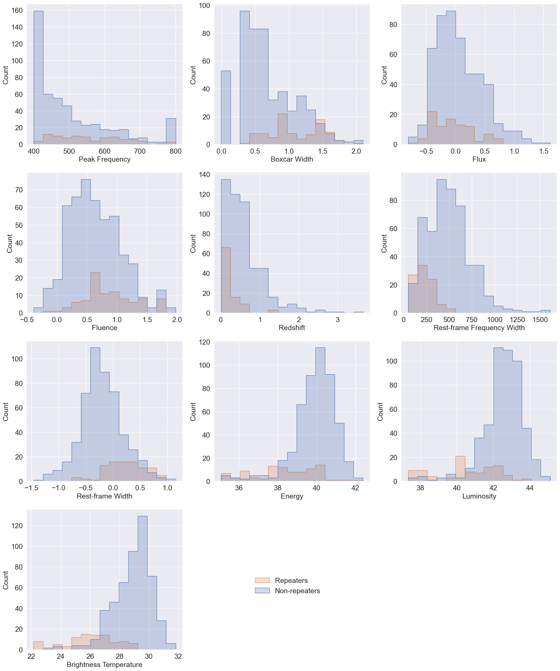
Figure 1: Comparison of the input features distributions between repeating and non-repeating FRBs.

3 Methods

Two kinds of unsupervised machine learning methods, clustering and dimensionality reduction, are used in this paper. Dimensionality reduction algorithms learn high-dimensional data sets and automatically transform them into a low-dimensional space. Clustering algorithms group a set of data points into clusters based on their similarities. In practice, high-dimension data are usually first visualized by dimensionality reduction to a lower dimension. Then, clustering methods are used to identify clusters of the data points, after which we can label them manually.

We utilize two kinds of dimensionality reduction algorithms, linear and manifold-based ones (Cayton, 2005), in three different workflows. In each workflow, we first input the FRBs with 10 features derived in section 2 into dimensionality reduction methods to transfer them to the lower dimension. To better illustrate the results, we visualize them in a two-dimensional space. Therefore, for all dimensionality reduction algorithms used in this paper, we set the corresponding hyperparameter n_components equal to 2. Note that in all the results of dimensional reduction shown in the figures, in order to compare with the cluster results, we color the repeaters in red and the non-repeaters in blue. However, we do not input the observed repetition of FRBs into the algorithms. Then, since the data points in the plot display some degree of clustering, we utilize clustering methods to identify them. Finally, to reveal the importance of the features in unsupervised machine learning, we deduce feature correlation from Mutual Information (MI). All the values of the hyperparameters used in this study are presented in Appendix A. We list them in Table A and Table 3, for dimensionality reduction and clustering respectively.

3.1 Dimensionality Reduction

3.1.1 Principal Component Analysis (PCA)

Principal Components Analysis (PCA) (Jolliffe, 1986; Hotelling, 1933) is one of the most popular algorithms for linear dimensionality reduction. Given a data set, the PCA algorithm finds the directions (vectors) along which the data has a maximum variance and deduces the relative importance of these directions. Then, the algorithm keeps the most principal vectors as the principal components according to their importance. The number of reserved vectors is decided by the hyperparameter n_components.

Apart from n_components, in the PCA algorithm, we adopt other hyperparameters in default values. Since PCA is a linear method based on variances, we preprocess the data to standardize features by removing the mean and scaling to unit variance and then putting them into the PCA algorithm. The dimensional reduction result of PCA is shown in Figure 2. Repeaters and non-repeaters are clearly in different regions.

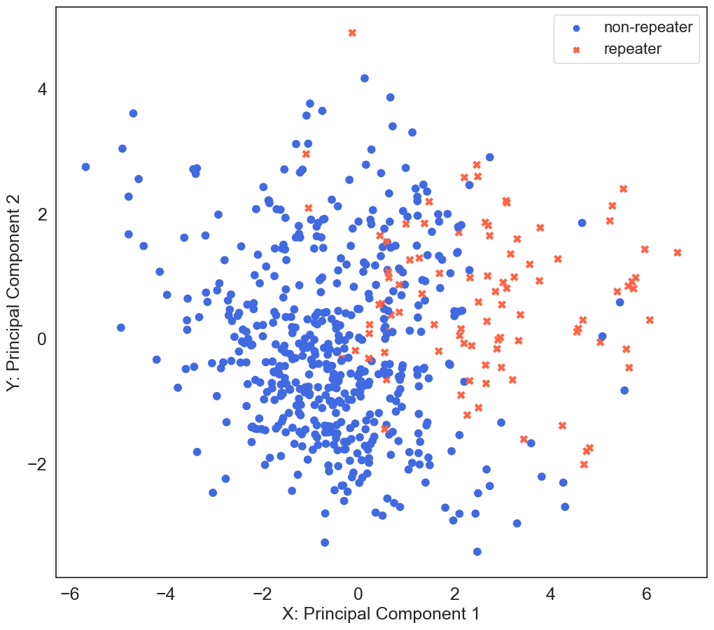
Figure 2: Dimensionality reduction results from PCA. The samples of repeating FRBs and non-repeating FRBs are clearly distributed in different regions.

3.1.2 t-distributed Stochastic Neighbor Embedding (t-SNE)

T-distributed Stochastic Neighbor Embedding (t-SNE) (van der Maaten & Hinton, 2008; van der Maaten, 2014) is a manifold dimensionality reduction algorithm. It is based on Stochastic Neighbor Embedding (SNE) (Hinton & Roweis, 2002). Stochastic Neighbor Embedding (SNE) first converts the high-dimensional Euclidean distances into conditional probabilities. Then, SNE algorithms minimize the sum of Kullback-Leibler divergences by optimizing the cost function with gradient descent. However, SNE is prone to the “crowding problem” which is common in manifold algorithms and can show crowded point distributions in the two-dimensional space. In this case, t-SNE modifies the Gaussian distribution used in the probability of SNE to a Student-t distribution. Compared with Gaussian distribution, t distribution has a heavy tail, causing two distant data points to increase their distance while transforming to a lower dimension. Therefore, t-SNE can avoid the crowding problem and its performance is greatly improved.

Perplexity is one of the critical hyperparameters in t-SNE. It is related to the number of nearest neighbors. A large value of perplexity means a more global view of the manifold, while a small value shows the local structure of the input. According to Oskolkov (2019), $\mathrm{perplexity}\sim N^{1/2}$ is a reasonable value, while $N$ is the number of input samples. Thus, we set perplexity equal to 24. Another hyperparameter n_iter stands for the number of iterations in the optimization as mentioned before. In gradient descent, if the number of iterations is large enough, the parameters will be closer to their local optimal solutions but cost much time. Here we set n_iter as 1000, which is enough number for the iterations. The dimensionality reduction results are plotted in Figure 3. Most repeating FRBs are on the right-hand side and generally reside in the same clusters.

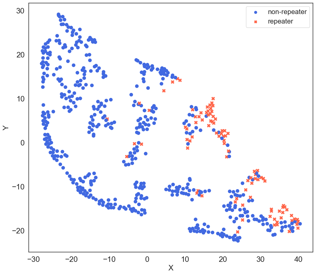
Figure 3: Dimensionality reduction results from t-SNE. Most repeating FRBs are on the right-hand side and generally reside in the same clusters.

3.1.3 Uniform Manifold Approximation and Projection (UMAP)

Uniform Manifold Approximation and Projection (UMAP) (McInnes & Healy, 2018) is another manifold learning technique for dimensionality reduction. As a manifold algorithm, the theoretical foundation for UMAP is also based on Riemannian geometry. However, UMAP assumes that the input data is uniformly distributed on the manifold. Another difference in UMAP is the modification from metric spaces to fuzzy topological representations.

Two hyperparameters n_neighbors and min_dist count here. Similar to perplexity in t-SNE, n_neighbors corresponds to the size of the local neighborhood used for manifold approximation. A higher value of n_neighbors results in a more global view of the manifold. Similarly, we adopt n_neighbors to be 24. Another vital hyperparameter min_dist represents the effective minimum distance among embedded points. To recognize various clusters without interference by the internal points in each cluster, for UMAP, a small value should be set. Therefore, we adopt min_dist to be 0 based on our experience. UMAP’s results are shown in Figure 4. Similar to t-SNE, most repeating FRBs are on the right-hand side and generally reside in the same clusters.

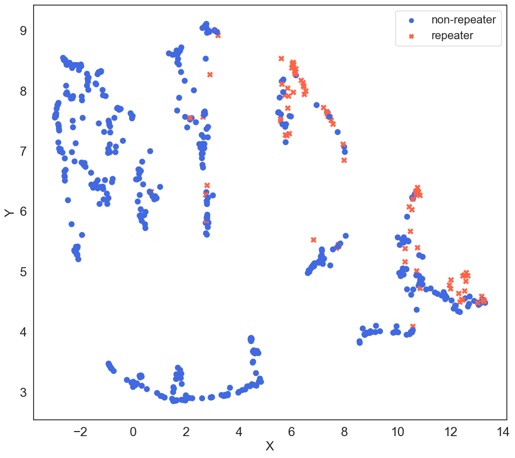
Figure 4: Dimensionality reduction results from UMAP. Similar to t-SNE, most repeating FRBs are on the right-hand side and generally reside in the same clusters.

3.2 Clustering

3.2.1 $k$-means

The $k$-means algorithm (Lloyd, 1982; MacQueen, 1967) groups the data points into clusters by minimizing the sum of squares of Euclidean distances between the geometric points and their centroids. It first initializes $k$ points as cluster centers and then optimizes their positions until they reach the real centers of each cluster. Because $k$-means is based on the distance from each point to their centers, it performs well in circular-like clusters but fails to identify clusters with strange shapes such as curved shapes. Therefore, we use $k$-means in dealing with linear-based dimensionality reduction algorithms PCA.

A vital hyperparameter in $k$-means is n_clusters, which refers to how many cluster centers are present in the model. In this paper, we calculate the silhouette coefficient of $k$-means with different n_clusters to determine the best number of clusters. Silhouette coefficient has long been used to evaluate the quality of clustering. It ranges from -1 to 1, and a higher value stands for more coherent clusters. The silhouette coefficient for one of the data points $o_{i}$ is defined as (Rousseeuw, 1987; Han et al., 2012; Belyadi & Haghighat, 2021):

$$s(o_{i})=\frac{b(o_{i})-a(o_{i})}{max\{a(o_{i}),b(o_{i})\}},$$ (8)

where $a(o_{i})$ is the average distance between $o_{i}$ and all other data points within the same cluster, while $b(o_{i})$ refers to the average distance between $o_{i}$ and all other data points outside the cluster to which $o_{i}$ belongs. For the clustering metric, the silhouette coefficient is the average value for all data points. If a clustering method performs well, each cluster should be tightly clustered and have a long distance from other clusters. In this case, its silhouette coefficient will be close to 1. The values of silhouette coefficients in various n_clusters of $k$-means are shown in Figure 5. We choose n_clusters equal to 2 corresponding to the maximum value of the silhouette coefficient and show the cluster result in Figure 6.

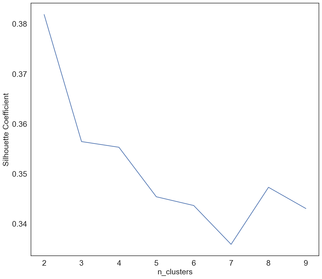
Figure 5: Silhouette coefficients of $k$-means after PCA with respect to different number of clusters. The maximum value of silhouette coefficient implies 2 clusters in PCA space and the corresponding hyperparameter for $k$-means.

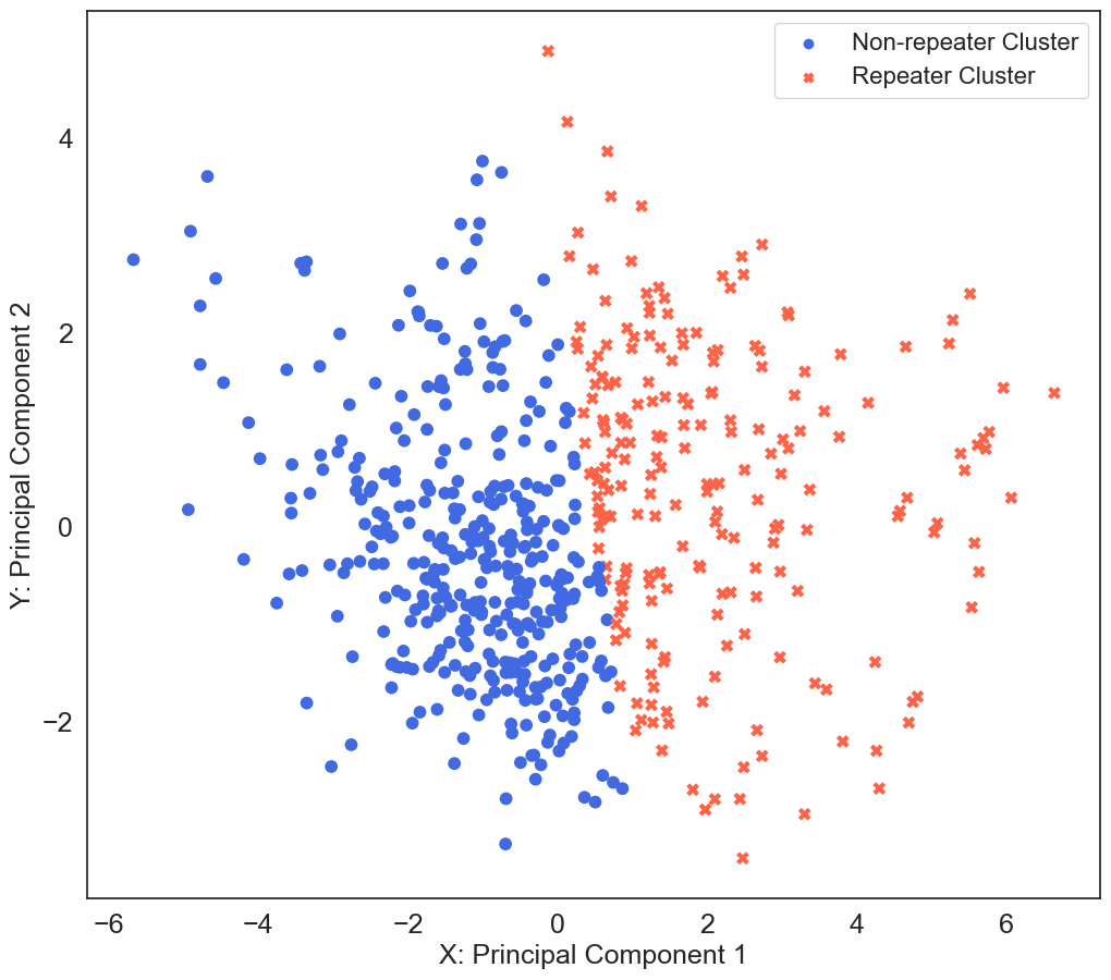
Figure 6: The $k$-means clustering result in PCA space. The right cluster, containing a higher ratio of repeaters, is identified as the repeater cluster, while the left one is identified as the non-repeater cluster. The two clusters are consistent with the distribution of observed repeaters and non-repeaters in Figure 2.

3.2.2 Hierarchical Density-Based Spatial Clustering of Applications with Noise (HDBSCAN)

Another algorithm we use to cluster the data points is Hierarchical Density-Based Spatial Clustering of Applications with Noise (HDBSCAN)(Campello et al., 2013; McInnes & Healy, 2017; McInnes et al., 2017). HDBSCAN is an algorithm improved from Density-Based Spatial Clustering of Applications with Noise (DBSCAN) (Ester et al., 1996) and combined with Hierarchical Clustering (Han et al., 2012; Belyadi & Haghighat, 2021). DBSCAN utlizes two hyper-parameters to estimate the density in an area: $\varepsilon$ and MinPts. $\varepsilon$ is the radius defined as the neighborhood for a point, and MinPts is defined as the critical number of data points within the neighborhood. Three types of points are then defined:

1. Core point: a point that has more data points within its neighborhood than MinPts.

2. Border point: a point in the neighborhood of one core point but the number of data points within its neighborhood is fewer than MinPts.

3. Noise point: a point that is neither a core point nor a border point.

With specific values of $\varepsilon$ and MinPts, DBSCAN automatically clusters the data points based on the area covering the core points and border points without any parameter corresponding to the number of clusters. Hierarchical clustering is a series of methods that start from the cluster of each point and merge to a larger cluster, or from a single cluster and split to smaller subclusters, according to the change of the criterion value. HDBSCAN is refined from DBSCAN in simplifying the density measurement and combining with hierarchical clustering while scanning the densities. It chooses the clusters based on the hierarchical structure from such steps.

HDBSCAN performs well after manifold dimensionality reduction over $k$-means due to the strange shapes of the groups. Those groups usually are not in circles or follow Gaussian distribution. $k$-means or other clustering algorithms fail to apply. Therefore, we utilize HDBSCAN after the manifold algorithms t-SNE and UMAP. Similar to DBSCAN, HDBSCAN does not need to know the number of clusters in advance. HDBSCAN automatically determines the number of clusters while clustering the points. Besides, HDBSCAN can recognize outlier points as noises.

We first input data into the t-SNE or UMAP algorithms to reduce the dimension and then utilize the HDBSCAN algorithm to label the clusters. The clusters that only include non-repeaters are recognized as "non-repeater clusters". The clusters containing more than a single-digit number (we defined 15% as the criterion) of repeaters are classified as "repeater clusters". Non-repeaters in repeater clusters can then be treated as hidden repeaters. As for the clusters that only have a few repeaters and the ratio is not enough for 15%, they are labeled as "other clusters". The single-digit repeaters in these clusters may be misclassified due to the inaccuracies of their input features, or indicate that the clusters are repeater ones. Further observation is required.

The cluster results of t-SNE and UMAP are shown respectively in Figure 7 and Figure 8. To better visualize them, we color the repeater clusters in red color series, other clusters in green color series, and non-repeater clusters in blue color series.

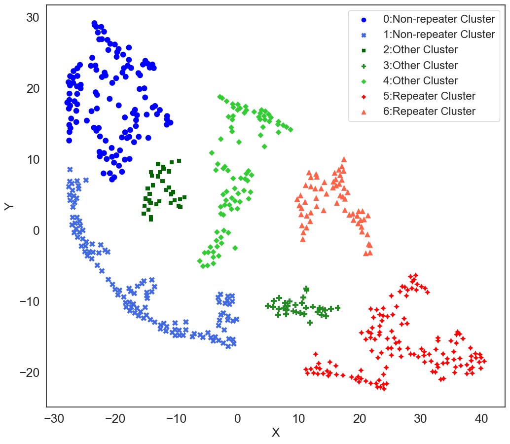
Figure 7: Clustering results of HDBSCAN in the t-SNE plane. Non-repeater clusters are marked in blue, while repeater clusters are marked in red. Other clusters are marked in green.

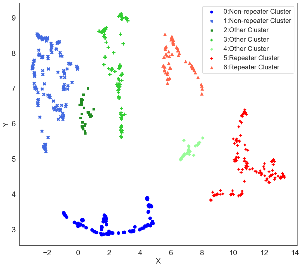
Figure 8: Clustering results of HDBSCAN in the UMAP plane. Non-repeater clusters are marked in blue, while repeater clusters are marked in red. Other clusters are marked in green.

3.3 Feature Correlations: Mutual Information

After dimensionality reduction and clustering, the data points are visualized in two-dimensional spaces and are clustered based on their similarities. However, the correlation between the final result and the input features is still unknown. In order to unravel the correlation and the importance of features in different algorithms, Mutual Information regression in the scikit-learn library is used to estimate the Mutual Information between the features and the coordinates (Rovira et al., 2022).

Mutual Information is first proposed by Shannon (1948) and is widely adopted in machine learning since Battiti (1994). MI is calculated from the Kullback–Leibler divergence between the joint distribution and the product of the marginal distributions of two variables. For a pair of random variables $X$ and $Y$, MI can be written as:

$$I(X;Y)=\int\int P_{(X,Y)}(x,y)\log\frac{P_{(X,Y)}(x,y)}{P_{X}(x)P_{Y}(y)}\,dx\,dy,$$ (9)

where $P_{(X,Y)}$ is the joint probability mass function of $X$ and $Y$, and $P_{X}$ and $P_{Y}$ are the marginal probability mass functions of $X$ and $Y$, respectively. It is a non-negative value and measures the mutual dependence between the two variables, as a higher MI score implies a higher dependence.

In this paper, we first compute the MI scores of each cluster to estimate the feature correlation for the clusters. Then, we stack the MI scores of the clusters in each method to show the importance of features in dimensionality reduction. To better illustrate them, we paint the bars in the same color series as clustering results reported in section 3.2. Note that for each feature, the left bar correlates with the $x$-axis while the right bar is related to the $y$-axis. The MI scores of PCA, t-SNE and UMAP are shown in Figures 9, 10 and 11.

In Figure 9, the MI scores of the linear method PCA are relatively balanced between the repeater cluster and non-repeater cluster, which is consistent with the clustering results in Figure 6. Generally, boxcar width, redshift, energy, luminosity and brightness temperature are the most important features in PCA. The MI scores also reflect the variances of features in the principal vectors.

For the manifold methods t-SNE and UMAP, clustered by HDBSCAN, their feature correlation shown in Figure 10 and 11 are similar. For non-repeater clusters in blue, peak frequency, redshift and rest-frame frequency width are the most dominant features, while redshift is not as significant in the repeater clusters colored red. On the whole, peak frequency, redshift and rest-frame frequency width are the most important features.

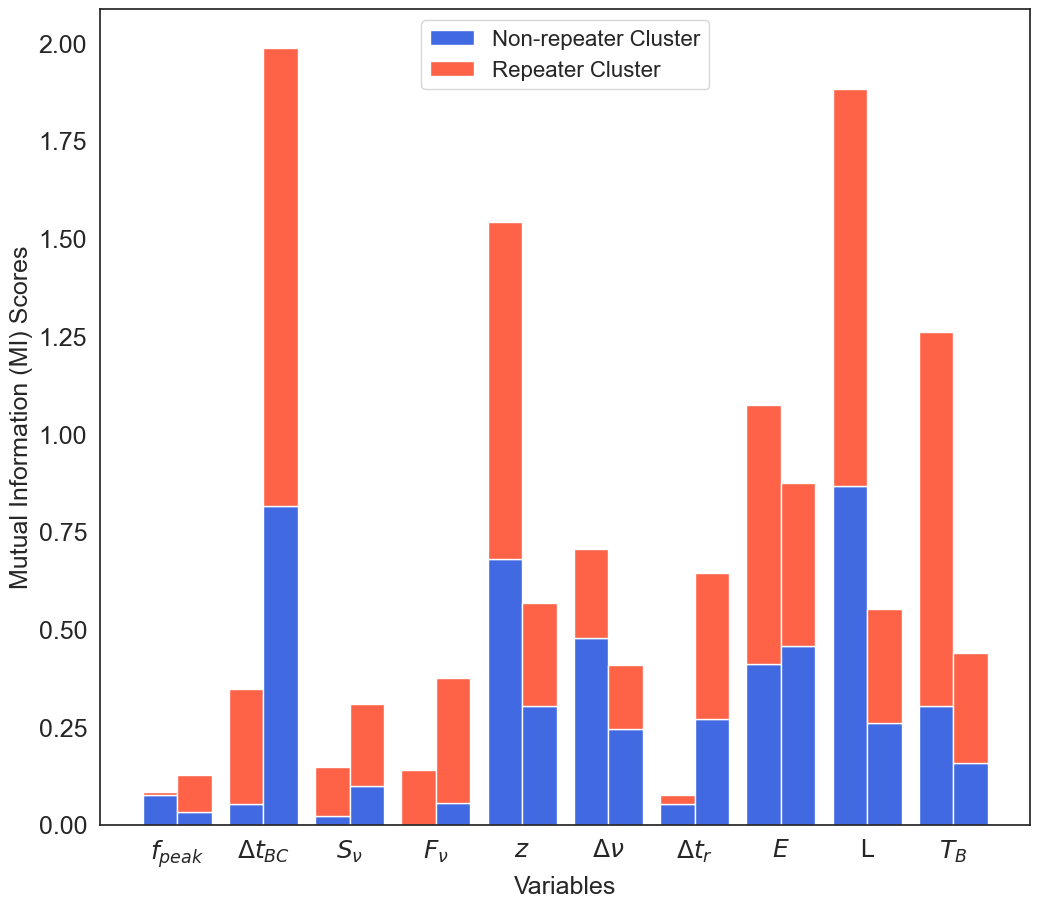
Figure 9: Feature correlation of PCA+$k$-means. The left bar correlates with the $x$-axis while the right bar is related to the $y$-axis. Boxcar width, redshift, energy, luminosity and brightness temperature are the most important features in PCA.

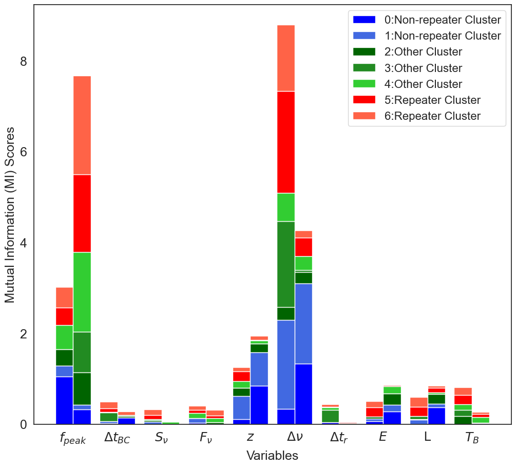
Figure 10: Feature correlation of t-SNE+HDBSCAN. For non-repeater clusters in blue, peak frequency, redshift and rest-frame frequency width are the most dominant features, while redshift is not as significant in the repeater clusters colored red. On the whole, peak frequency, redshift and rest-frame frequency width are the most important features.

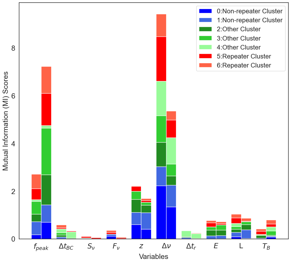
Figure 11: Features correlation of UMAP+HDBSCAN. For non-repeater clusters in blue, peak frequency, redshift and rest-frame frequency width are the most dominant features, while redshift is not as significant in the repeater clusters colored red. On the whole, peak frequency, redshift and rest-frame frequency width are the most important features.

4 Analysis and Discussion

In section 3, we presented the models we selected and their visualized results. Since they are all unsupervised machine learning methods, no information on burst identification (whether an FRB is a repeater or an apparent non-repeater) is included. The algorithms only study their features and transform them into different clusters. Then, by comparing with the observed identities from the CHIME catalog, we consider various clusters as repeaters, non-repeaters, or others. In this section, we will first introduce some metrics to evaluate the performance of machine learning algorithms. Then, we delineate the similarities between manifold methods. After that, we combine all the results, deduce their weight vector to evaluate their significance, and rank each FRB to obtain its classified label. Finally, we list our most credible repeater candidates.

4.1 Evaluation of different models

In machine learning classification, outputs are written as the following forms:

1. True positive (TP):

   Predicted to be positive, and is truly positive.

2. True negative (TN):

   Predicted to be negative, and is truly negative.

3. False positive (FP):

   Predicted to be positive, but is actually negative.

4. False negative (FN):

   Predicted to be negative, but is actually positive.

In our work, we define the positive as repeaters, while the negative as other than repeaters (including non-repeaters clusters and other clusters). Also, under the definition, repeater candidates are False Positives (FPs).

Based on the definition of outcomes and our classification results, we can get a general sense that if a model covers almost all the actual repeaters in its predicted repeaters and includes a few repeater candidates (FP here), this model can be considered well-performing. Precision and recall are two metrics that meet our needs.

• Precision

  $$P=Precision=\frac{TP}{TP+FP}$$ (10)

• Recall

  $$R=Recall=\frac{TP}{TP+FN}$$ (11)

Notice that we do not adopt accuracy here, which is defined as $(TP+TN)/(TP+FN+FP+TN)$. This is because we need a model with a high ratio of TP, and a low ratio of FN and FP, rather than the ratio of TN. Even if each model categorizes all the points as non-repeaters, $Accuracy$ will be highly scored.

To combine both precision and recall, we adopt F-measure to evaluate the models. The full definition of the F-measure is given by (Chinchor, 1992; Blair, 1979):

$$F_{\beta}=\frac{(1+\beta^{2})PR}{\beta^{2}P+R}\qquad(0\leq\beta\leq+\infty).$$ (12)

Here, values of $\beta$ represent weights of $precision$ and $recall$ (Sasaki, 2007). Specially, if $\beta=1$, $F_{\beta}$ falls back to the classic $F_{1}-score$, where $precision$ and $recall$ are considered equally. Apart from that, if $\beta<1$, $F_{\beta}$ becomes more dominated by $precision$ and if $\beta>1$, $F_{\beta}$ are more recall-oriented. For FRBs, apparently non-repeaters may actually be repeaters, while observed repeaters should not be classified as non-repeaters. In this case, $Recall$ must be a priority and preferably to be close to 100%. Therefore, We adopt $\beta=2$ and calculate the metrics in Table 1. All workflows show $F_{2}-score$ higher than 0.70, indicating good performances.

Table 1: Evaluation metrics for each model. The high scores in $F_{2}$ indicate good performances of the three workflows.

Method	TP	FN(Misclassified Repeaters)	FP(Repeaters Candidates)	TN	$Recall$	$Precision$	$F_{2}$
PCA+$k$-means	85	9	127	373	0.9042	0.4009	0.7227
t-SNE+HDBSCAN	81	13	117	383	0.8617	0.4091	0.7056
UMAP+HDBSCAN	81	13	117	383	0.8617	0.4041	0.7056

4.2 Manifold Structures across Methods

Until now, the analysis for the results and evaluations are all given individually. But since we employ different algorithms and visualize them, an interesting practice is to study the structures across different methods. Especially, manifold results in Figure 7 and Figure 8 seem to share some groups with similar shapes. A simple idea is to plot one classification set on another reduced dimensional plane to check if those clusters are the same FRBs. Here we plot the t-SNE result in UMAP space in Figure 12 and the exchange condition in Figure 13. In both figures, the color series across the mehods are generally the same, only a few points on the edge of clusters may be in different clusters.

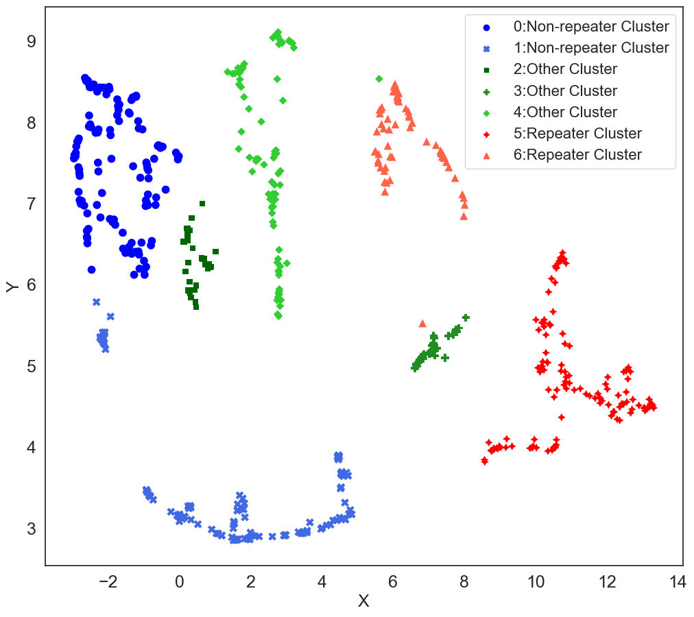
Figure 12: Data points in UMAP plane colored with the cluster labels identified by t-SNE and HDBSCAN. Only two points are in the different series of clusters.

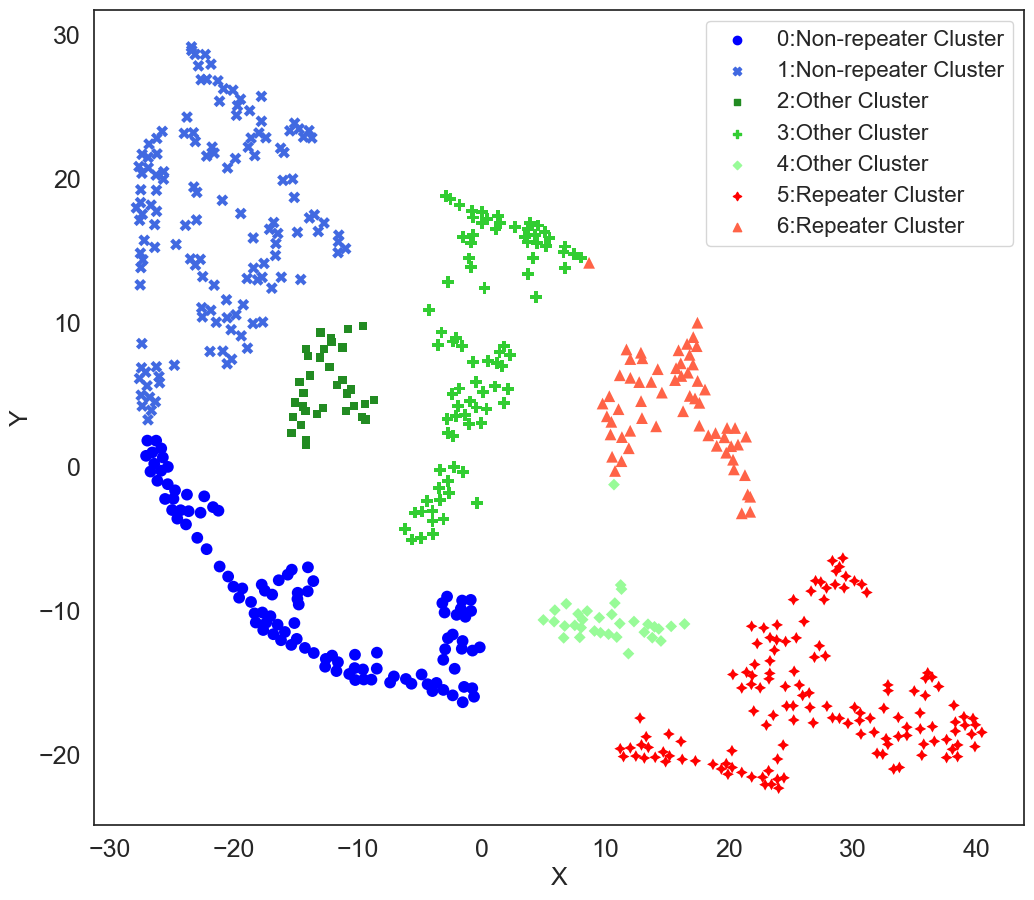
Figure 13: Data points in t-SNE plane colored with the cluster labels identified by UMAP and HDBSCAN. Only two points are in the different series of clusters.

4.3 Categories of FRBs

Since the physical origin of FRBs is not identified, we do not know how many categories of FRBs are there. Unsupervised machine learning algorithms learn the data from their features without any premise of repeaters and non-repeaters, those algorithms open a window to uncover the number of categories and also the traits of each category.

In section 3.2.1, we calculated silhouette coefficient to determine the number of clusters. Here, we can also deduce the coefficients directly in the raw high-dimensional space. The result shown in Figure 14 indicates 2 main categories of FRBs, while 5 or 6 is also possible albeit with lower significance.

Another clue is from the manifold methods in section 3.1.2 and section 3.1.3, both algorithms tend to output 7 categories in the two-dimensional space. In order to reveal the features of each cluster more specifically, considering the similar classified results of manifold methods discussed in section 4.2, we plot the features again but in hues of the labels given by t-SNE in Figure 15. Note that peak frequency and rest-frame frequency width of most FRBs in clusters 1 and 5 are at the observational limit of CHIME, which might be two false sub-categories because of observational biases, indicating that there might be 5 to 7 species of FRBs. Compared with other research applied unsupervised machine learning to Gamma-ray Bursts (Jespersen et al., 2020), which just includes two clear categories, the number of species in FRBs might imply a more complicated physical origin than GRBs.

In Figure 15, the repeater clusters share smaller values in redshift, rest-frame frequency width, energy, luminosity and brightness temperature, and slightly larger values in boxcar width, which is consistent with the observed distributions of repeaters in Figure 1. Specifically, in the non-repeater clusters, cluster 0 is the non-repeater cluster with relatively higher peak frequency, redshift, rest-frame frequency width, energy and luminosity. For the repeater clusters, cluster 6 is the repeater cluster with higher peak frequency, fluence and rest-frame frequency width. For the other clusters, their properties lie between the repeater clusters and non-repeater clusters. While the non-repeaters in the repeater clusters are those repeater candidates we want, those in the other clusters also need follow-up observations to identify their real classes.

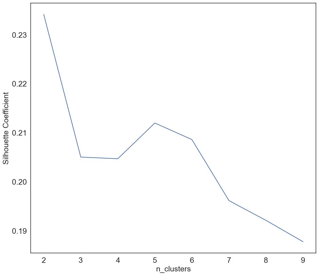
Figure 14: Silhouette coefficients of $k$-means with respect to different number of clusters, directly in the raw space without PCA. In addition to the maximum value at 2 clusters, the plateau corresponding to 5 and 6 clusters implies possible subcategories with lower significance.

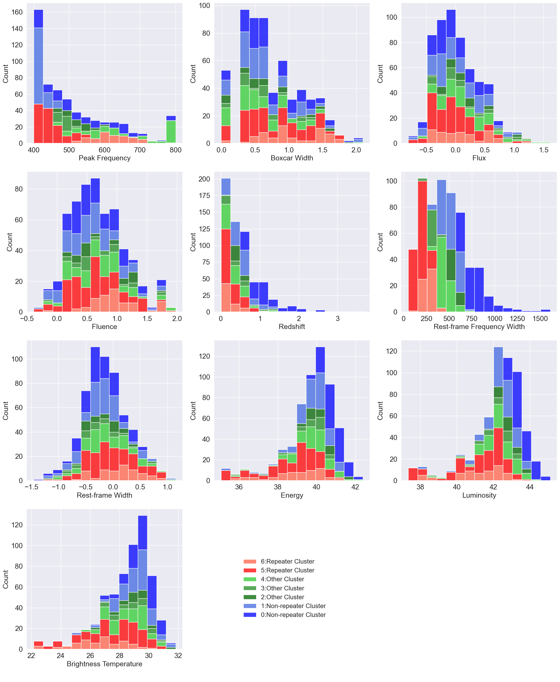
Figure 15: Input features of FRBs in the labels given by t-SNE and HDBSCAN. The different distributions of the clusters imply the corresponding categories.

4.4 Repeater candidates from the Combination of Algorithms

We used various algorithms to classify FRBs in the first CHIME/FRB catalog. Since they all provide a set of hidden repeaters, their intersection can be reckoned as the most credible repeaters candidates. Thus, we give the candidate list, hoping to assist future repeater search. Their basic information and features are listed in Table 2. We also cross compare with the repeater candidates identified using supervised methods (Paper I, Luo et al. (2022)) and box the overlapping candidates from the two papers. These should be the strongest candidates and we encourage close follow-up observations of these sources to detect their repeated bursts.

Table 2: Repeater candidates: the most plausible candidates given by unsupervised machine learning methods. The boxed FRBs are also identified as repeater candidates in supervised methods (Paper I, Luo et al. (2022)). Sub num is the sub-burst number of FRBs in the first CHIME/FRB catalog. Description of the properties can be found in Section 2.

Name	Sub	RA	Dec	$\nu_{c}$	$\log\Delta t_{BC}$	$\log S_{\nu}$	$\log F_{\nu}$	$z$	$\Delta\nu$	$\log\Delta t_{r}$	$\log E$	$\log L$	$\log T_{B}$
	Num	∘	∘	$\mathrm{MHz}$	$\log$\mathrm{ms}$$	$\log$\mathrm{Jy}$$	$\log$\mathrm{Jy}\text{\,}\mathrm{ms}$$		$\mathrm{MHz}$	$\log$\mathrm{ms}$$	$\log$\mathrm{erg}$$	$\log$\mathrm{erg}\text{\,}{\mathrm{s}}^{-1}$$	$\log$\mathrm{K}$$
FRB20180907E	0	167.88	47.09	400.2	1.07	-0.14	0.84	0.312	178.54	0.500	39.85	41.99	27.89
FRB20180911A	0	99.55	84.62	400.2	0.29	0.20	0.41	0.085	216.59	-0.116	38.26	41.09	28.62
FRB20180915B	0	225.23	25.02	400.2	0.69	0.00	0.58	0.072	136.33	0.199	38.28	40.73	27.47
FRB20180920B	0	191.09	63.52	421.1	1.03	-0.46	0.23	0.401	116.53	0.221	39.49	41.95	27.83
FRB20180923A	0	327.61	71.92	468.9	0.29	-0.12	0.08	0.026	177.17	-0.835	36.96	39.77	27.12
FRB20180923C	0	239.14	22.85	420.5	0.29	-0.05	0.14	0.059	291.70	-0.520	37.69	40.53	28.01
FRB20180928A	0	312.95	30.85	400.2	0.47	0.13	0.40	0.002	92.11	-0.571	35.08	37.81	25.02
FRB20181013E	0	307.28	69.02	400.2	0.47	-0.21	0.31	0.208	269.06	-0.147	38.96	41.52	28.66
$$FRB20181017B$$	0	237.76	78.50	593.2	1.11	0.03	0.81	0.207	247.97	0.282	39.63	41.92	27.27
$$FRB20181030E$$	0	135.67	8.89	470.5	0.77	0.30	0.80	0.013	166.76	-0.404	37.09	39.59	25.99
FRB20181125A	0	147.94	33.93	434.5	1.17	-0.41	0.51	0.171	156.33	0.039	39.02	41.17	26.81
FRB20181125A	1	147.94	33.93	436.6	1.17	-0.41	0.51	0.171	177.76	0.090	39.02	41.17	26.81
FRB20181125A	2	147.94	33.93	426.5	1.17	-0.41	0.51	0.171	141.34	0.130	39.01	41.16	26.83
FRB20181130A	0	355.19	46.49	412.1	-0.01	-0.01	0.10	0.033	119.55	-0.333	37.14	40.04	28.16
FRB20181214A	0	70.00	43.07	435.0	0.47	-0.81	-0.39	0.231	116.19	-0.363	38.39	41.06	28.08
FRB20181220A	0	346.11	48.43	400.2	0.47	0.12	0.48	0.002	196.64	-0.362	35.16	37.81	25.02
$$FRB20181221A$$	0	230.58	25.86	510.1	0.69	0.10	0.76	0.240	170.15	-0.216	39.65	42.07	28.44
FRB20181226E	0	303.56	73.64	400.2	0.47	-0.32	0.13	0.178	186.23	-0.003	38.64	41.26	28.41
$$FRB20181229B$$	0	238.37	19.78	445.5	1.31	-0.38	0.69	0.320	154.80	0.406	39.77	41.83	27.09
$$FRB20181231B$$	0	128.77	55.99	657.7	0.47	-0.05	0.37	0.066	276.56	-0.500	38.22	40.82	27.37
FRB20190106B	0	335.63	46.13	452.1	0.29	0.23	0.58	0.098	157.27	-0.278	38.61	41.30	28.67
$$FRB20190109B$$	0	253.47	1.25	408.1	0.84	0.08	0.48	0.009	93.05	-0.473	36.40	39.00	25.45
FRB20190110C	0	246.98	41.42	427.4	0.47	-0.19	0.15	0.112	86.17	-0.455	38.27	40.98	28.06
FRB20190111A	2	217.00	26.78	400.2	0.77	0.56	1.23	0.066	251.25	-0.130	38.87	41.22	27.81
$$FRB20190112A$$	0	257.98	61.20	697.7	0.99	0.15	1.21	0.348	317.48	0.085	40.56	42.63	27.94
$$FRB20190129A$$	0	45.06	21.42	707.7	0.95	-0.31	0.70	0.404	347.23	-0.094	40.19	42.33	27.70
FRB20190204A	0	161.33	61.53	418.2	0.90	-0.62	0.18	0.382	217.88	0.117	39.39	41.73	27.90
$$FRB20190206A$$	0	244.85	9.36	534.5	0.77	0.15	0.96	0.062	213.84	-0.121	38.66	40.87	27.08
$$FRB20190218B$$	0	268.70	17.93	588.0	1.25	-0.24	0.77	0.442	334.17	0.153	40.26	42.41	27.41
FRB20190220A	0	237.21	74.16	400.2	0.29	-0.47	-0.17	0.098	265.91	-0.300	37.81	40.55	28.08
FRB20190221A	0	132.60	9.90	444.8	0.47	0.09	0.37	0.092	225.37	-0.052	38.34	41.10	28.14
FRB20190222B	0	160.69	19.62	400.2	1.34	-0.40	0.64	0.439	278.25	0.024	39.96	42.08	27.41
FRB20190223A	0	64.72	87.65	444.8	0.59	-0.33	0.20	0.286	149.61	-0.227	39.18	41.76	28.48
FRB20190228A	0	183.48	22.90	664.7	1.48	0.25	1.55	0.365	357.33	0.217	40.93	42.76	27.15
FRB20190308C	0	188.36	44.39	453.4	1.34	-0.33	0.68	0.454	218.85	-0.561	40.09	42.24	27.40
FRB20190308C	1	188.36	44.39	449.0	1.34	-0.33	0.68	0.454	211.58	-0.422	40.08	42.24	27.41
FRB20190308B	0	38.59	83.62	477.2	0.29	0.05	0.14	0.015	190.59	-0.737	36.57	39.48	26.81
FRB20190308B	1	38.59	83.62	455.5	0.29	0.05	0.14	0.015	187.95	-0.291	36.55	39.46	26.85
FRB20190323D	0	56.88	46.93	400.2	1.11	-0.43	0.40	0.593	204.86	0.533	39.99	42.36	28.10
$$FRB20190329A$$	0	65.54	73.63	432.3	1.07	-0.28	0.35	0.002	73.87	0.016	35.06	37.43	23.34
FRB20190403E	0	220.22	86.54	620.6	1.27	0.59	1.88	0.099	348.03	0.301	40.06	41.81	26.81
$$FRB20190409B$$	0	126.65	63.47	545.5	1.48	-0.41	0.83	0.175	336.98	0.299	39.46	41.29	26.01
$$FRB20190410A$$	0	263.47	-2.37	515.7	0.84	0.20	0.76	0.073	182.92	-0.026	38.59	41.06	27.18
$$FRB20190412B$$	0	285.65	19.25	400.2	1.63	-0.17	1.11	0.015	228.59	0.826	37.42	39.15	24.04
FRB20190418A	0	65.79	16.04	400.2	0.29	0.00	0.34	0.019	182.96	-0.159	36.89	39.55	27.11
FRB20190419A	0	104.98	64.88	407.1	0.59	-0.39	-0.11	0.341	185.53	0.140	38.99	41.84	28.66
FRB20190422A	0	48.56	35.15	626.1	1.47	-0.22	0.96	0.335	373.37	0.382	40.23	42.18	26.68
$$FRB20190422A$$	1	48.56	35.15	612.3	1.47	-0.22	0.96	0.335	312.63	0.238	40.22	42.17	26.70
FRB20190423A	1	179.68	55.25	400.2	0.77	1.03	1.74	0.143	220.29	0.316	40.06	42.40	28.96
$$FRB20190423B$$	0	298.58	26.19	537.6	0.99	-0.06	0.85	0.003	159.79	0.395	35.93	38.03	23.81
$$FRB20190423B$$	1	298.58	26.19	524.6	0.99	-0.06	0.85	0.003	148.96	0.928	35.92	38.02	23.83
$$FRB20190429B$$	0	329.93	3.96	422.4	1.22	-0.13	0.70	0.194	50.64	0.728	39.31	41.56	27.12
FRB20190430A	0	77.70	87.01	433.8	1.29	-0.12	0.89	0.228	214.13	0.440	39.65	41.73	27.10
FRB20190517C	0	87.50	26.62	435.5	0.29	0.49	0.94	0.063	147.92	-0.450	38.56	41.14	28.57
$$FRB20190527A$$	0	12.45	7.99	484.7	1.76	-0.33	1.00	0.537	205.46	0.240	40.59	42.44	26.65
FRB20190527A	1	12.45	7.99	449.1	1.76	-0.33	1.00	0.537	172.11	0.206	40.55	42.41	26.72
FRB20190531C	0	331.14	43.00	453.0	0.47	-0.43	0.08	0.304	183.03	0.046	39.12	41.73	28.67
FRB20190601B	0	17.88	23.82	429.5	1.39	0.00	1.11	0.754	202.91	0.362	40.94	43.07	28.11
FRB20190601C	0	88.52	28.47	517.0	0.77	0.12	0.76	0.175	223.54	-0.235	39.37	41.80	28.01
FRB20190601C	1	88.52	28.47	502.2	0.77	0.12	0.76	0.175	201.91	-0.363	39.36	41.79	28.03
$$FRB20190609A$$	1	345.30	87.94	600.5	0.69	0.56	1.02	0.200	267.97	0.247	39.81	42.43	28.59
FRB20190617A	0	178.60	83.87	409.9	0.69	0.76	1.32	0.065	290.64	0.146	38.94	41.41	28.13
FRB20190617B	0	56.43	1.16	459.3	1.14	0.00	0.96	0.166	217.37	0.813	39.47	41.57	27.20
FRB20190618A	0	321.25	25.44	419.3	0.29	0.38	0.63	0.068	149.73	-0.290	38.31	41.08	28.56
FRB20190625A	0	227.91	32.88	400.2	1.76	-0.46	1.08	0.225	293.38	0.505	39.80	41.35	25.89

5 Conclusions

Classifying FRBs as repeaters or non-repeaters has been a challenging problem. In this paper, we utilize unsupervised machine learning to learn the features of the FRBs in the first CHIME/FRB catalog and attempt to reveal their hidden properties. Most algorithms show classification results coincident with the groups of repeaters and non-repeaters. As a result, we draw the following conclusion:

• Repeaters and non-repeaters have different distributions in many features.

• Unsupervised machine learning algorithms, without the input of the observed identification of FRBs, can classify FRBs into clusters that have high correspondence with repeaters and non-repeaters. This suggests that repeaters and non-repeaters indeed belong to different categories.

• In addition to spotting the two most significant categories of repeaters and non-repeaters, unsupervised learning methods also imply that there may exist 5 to 7 subspecies based on their traits.

• Learning from multiple parameters, unsupervised machine learning identifies some hidden repeaters from the apparently non-repeaters. Many of such candidates overlap with the candidates identified from supervised machine learning methods (Paper I, Luo et al. (2022)). These candidates can be top targets for future follow-up observations to identify more repeaters from the CHIME archives.

Data Availability

The data we utilized in this paper from the first CHIME/FRB catalog is available at https://www.chime-frb.ca/catalog. The codes and other supplementary material are available at https://github.com/JiamingZhuge/FRB_ML_unsp.

Appendix A List of hyperparameters used

Name	Value
PCA
n_components	2
copy	True
whiten	False
svd_solver	’auto’
tol	0.0
iterated_power	’auto’
n_oversamples	10
power_iteration_normalizer	’auto’
random_state	None
t-SNE
n_components	2
perplexity	24
early_exaggeration	12
learning_rate	’auto’
n_iter	1000
n_iter_without_progress	300
min_grad_norm	1e-7
metric	’euclidean’
metric_params	None
init	’random’
verbose	0
random_state	45
method	’barnes_hut’
angle	0.5
n_jobs	None
square_distances	’deprecated’
UMAP
n_neighbors	24
n_components	2
metric	’euclidean’
metric_kwds	None
output_metric	’euclidean’
output_metric_kwds	None
n_epochs	None
learning_rate	1
init	’spectral’
min_dist	0
spread	1
low_memory	True
n_jobs	-1
set_op_mix_ratio	1
local_connectivity	1
repulsion_strength	1
negative_sample_rate	5
transform_queue_size	4
a	None
b	None
random_state	54
angular_rp_forest	False
target_n_neighbors	-1
target_metric	’categorical’
target_metric_kwds	None
target_weight	0.5
transform_seed	42
transform_mode	’embedding’
force_approximation_algorithm	False
verbose	False
tqdm_kwds	None
unique	False
densmap	False
dens_lambda	2
dens_frac	0.3
dens_var_shift	0.1
output_dens	False
disconnection_distance	None
precomputed_knn	(None,None,None)

Table 3: List of hyperparameters we used in the dimensionality reduction, including the default values.

Name	Value
$k$-means
n_clusters	2
init	’k-means++’
n_init	10
max_iter	300
tol	0.0001
verbose	0
random_state	4
copy_x	True
algorithm	’lloyd’
HDBSCAN
min_cluster_size(t-SNE)	32
min_samples(t-SNE)	2
min_cluster_size(UMAP)	22
min_samples(UMAP)	8
cluster_selection_epsilon	0
max_cluster_size	0
metric	’euclidean’
alpha	1
p	None
algorithm	’best’
leaf_size	40
memory	Memory(
	cachedir=None,
	verbose=0)
approx_min_span_tree	True
gen_min_span_tree	False
core_dist_n_jobs	4
cluster_selection_method	’eom’
allow_single_cluster	False
prediction_data	False
match_reference_implementation	False

Table 4: List of hyperparameters we used in the clustering, including the default values.

References

- Adámek & Armour (2020) Adámek K., Armour W., 2020, ApJS, 247, 56
- Agarwal et al. (2020) Agarwal D., Aggarwal K., Burke-Spolaor S., Lorimer D. R., Garver-Daniels N., 2020, MNRAS, 497, 1661
- Aggarwal (2021) Aggarwal K., 2021, ApJ, 920, L18
- Ai et al. (2021) Ai S., Gao H., Zhang B., 2021, ApJ, 906, L5
- Andersen et al. (2019) Andersen a. B. C., et al., 2019, ApJ, 885, L24
- Arcus et al. (2020) Arcus W. R., Macquart J.-P., Sammons M. W., James C. W., Ekers R. D., 2020, Monthly Notices of the Royal Astronomical Society, 501, 5319
- Battiti (1994) Battiti R., 1994, IEEE Transactions on Neural Networks, 5, 537
- Belyadi & Haghighat (2021) Belyadi H., Haghighat A., 2021, in Belyadi H., Haghighat A., eds, , Machine Learning Guide for Oil and Gas Using Python. Gulf Professional Publishing, pp 125–168, doi:https://doi.org/10.1016/B978-0-12-821929-4.00002-0, https://www.sciencedirect.com/science/article/pii/B9780128219294000020
- Blair (1979) Blair D. C., 1979, Journal of the American Society for Information Science, 30, 374
- Burke et al. (2019) Burke B. F., Graham-Smith F., Wilkinson P. N., 2019, An Introduction to Radio Astronomy, 4 edn. Cambridge University Press, doi:10.1017/9781316987506
- CHIME/FRB Collaboration et al. (2021) CHIME/FRB Collaboration et al., 2021, ApJS, 257, 59
- Caleb et al. (2019) Caleb M., Stappers B. W., Rajwade K., Flynn C., 2019, MNRAS, 484, 5500
- Campello et al. (2013) Campello R. J. G. B., Moulavi D., Sander J., 2013, in Pei J., Tseng V. S., Cao L., Motoda H., Xu G., eds, Advances in Knowledge Discovery and Data Mining. Springer Berlin Heidelberg, Berlin, Heidelberg, pp 160–172
- Cayton (2005) Cayton L., 2005, Univ. of California at San Diego Tech. Rep, 12, 1
- Chaikova et al. (2022) Chaikova A., Kostunin D., Popov S. B., 2022, arXiv e-prints, p. arXiv:2202.10076
- Chen et al. (2022) Chen B. H., Hashimoto T., Goto T., Kim S. J., Santos D. J. D., On A. Y. L., Lu T.-Y., Hsiao T. Y. Y., 2022, MNRAS, 509, 1227
- Chinchor (1992) Chinchor N., 1992, in Proceedings of the 4th Conference on Message Understanding. MUC4 ’92. Association for Computational Linguistics, USA, p. 22–29, doi:10.3115/1072064.1072067, https://doi.org/10.3115/1072064.1072067
- Connor & van Leeuwen (2018) Connor L., van Leeuwen J., 2018, AJ, 156, 256
- Cordes & Chatterjee (2019) Cordes J. M., Chatterjee S., 2019, ARA&A, 57, 417
- Cordes & Lazio (2002) Cordes J. M., Lazio T. J. W., 2002, arXiv e-prints, pp astro–ph/0207156
- Cui et al. (2022) Cui X.-H., et al., 2022, Ap&SS, 367, 66
- Deng & Zhang (2014) Deng W., Zhang B., 2014, The Astrophysical Journal, 783, L35
- Dolag et al. (2015) Dolag K., Gaensler B. M., Beck A. M., Beck M. C., 2015, Monthly Notices of the Royal Astronomical Society, 451, 4277
- Ester et al. (1996) Ester M., Kriegel H.-P., Sander J., Xu X., 1996, in Proceedings of the Second International Conference on Knowledge Discovery and Data Mining. KDD’96. AAAI Press, p. 226–231
- Farah et al. (2019) Farah W., et al., 2019, MNRAS, 488, 2989
- Fonseca et al. (2020) Fonseca E., et al., 2020, ApJ, 891, L6
- Fukugita et al. (1998) Fukugita M., Hogan C. J., Peebles P. J. E., 1998, ApJ, 503, 518
- Gao et al. (2014) Gao H., Li Z., Zhang B., 2014, The Astrophysical Journal, 788, 189
- Han et al. (2012) Han J., Kamber M., Pei J., 2012, in Han J., Kamber M., Pei J., eds, The Morgan Kaufmann Series in Data Management Systems, Data Mining (Third Edition), third edition edn, Morgan Kaufmann, Boston, pp 443–495, doi:https://doi.org/10.1016/B978-0-12-381479-1.00010-1, %****␣main.bbl␣Line␣175␣****https://www.sciencedirect.com/science/article/pii/B9780123814791000101
- Hashimoto et al. (2020) Hashimoto T., et al., 2020, MNRAS, 498, 3927
- Hinton & Roweis (2002) Hinton G. E., Roweis S. T., 2002, in NIPS.
- Hogg (1999) Hogg D. W., 1999, arXiv e-prints, pp astro–ph/9905116
- Hotelling (1933) Hotelling H., 1933, Journal of Educational Psychology, 24, 498
- James et al. (2022) James C. W., Prochaska J. X., Macquart J. P., North-Hickey F. O., Bannister K. W., Dunning A., 2022, MNRAS, 509, 4775
- Jespersen et al. (2020) Jespersen C. K., Severin J. B., Steinhardt C. L., Vinther J., Fynbo J. P. U., Selsing J., Watson D., 2020, ApJ, 896, L20
- Jolliffe (1986) Jolliffe I. T., 1986, Principal Component Analysis and Factor Analysis. Springer New York, New York, NY, pp 115–128, doi:10.1007/978-1-4757-1904-8_7, https://doi.org/10.1007/978-1-4757-1904-8_7
- Katz (2018) Katz J. I., 2018, Progress in Particle and Nuclear Physics, 103, 1
- Li et al. (2021a) Li D., et al., 2021a, Nature, 598, 267
- Li et al. (2021b) Li X. J., Dong X. F., Zhang Z. B., Li D., 2021b, ApJ, 923, 230
- Lloyd (1982) Lloyd S., 1982, IEEE Transactions on Information Theory, 28, 129
- Lorimer et al. (2007) Lorimer D. R., Bailes M., McLaughlin M. A., Narkevic D. J., Crawford F., 2007, Science, 318, 777
- Luo et al. (2022) Luo J.-W., Zhu-Ge J.-M., Zhang B., 2022, MNRAS, 518, 1629
- MacQueen (1967) MacQueen J., 1967, in Classification and analysis of multivariate observations. pp 281–297
- Macquart et al. (2020) Macquart J.-P., et al., 2020, Nature, 581, 391
- Marcote et al. (2020) Marcote B., et al., 2020, Nature, 577, 190
- McInnes & Healy (2017) McInnes L., Healy J., 2017, in 2017 IEEE International Conference on Data Mining Workshops (ICDMW). pp 33–42, doi:10.1109/ICDMW.2017.12
- McInnes & Healy (2018) McInnes L., Healy J., 2018, ArXiv, abs/1802.03426
- McInnes et al. (2017) McInnes L., Healy J., Astels S., 2017, The Journal of Open Source Software, 2
- Oskolkov (2019) Oskolkov N., 2019, How to tune hyperparameters of tSNE, https://towardsdatascience.com/how-to-tune-hyperparameters-of-tsne-7c0596a18868
- Palaniswamy et al. (2018) Palaniswamy D., Li Y., Zhang B., 2018, ApJ, 854, L12
- Petroff et al. (2019) Petroff E., Hessels J. W. T., Lorimer D. R., 2019, The Astronomy and Astrophysics Review, 27, 4
- Petroff et al. (2022) Petroff E., Hessels J. W. T., Lorimer D. R., 2022, A&ARv, 30, 2
- Planck Collaboration et al. (2020) Planck Collaboration et al., 2020, A&A, 641, A6
- Platts et al. (2019) Platts E., Weltman A., Walters A., Tendulkar S., Gordin J., Kandhai S., 2019, Physics Reports, 821, 1
- Pleunis et al. (2021) Pleunis Z., et al., 2021, ApJ, 923, 1
- Popov et al. (2018) Popov S. B., Postnov K. A., Pshirkov M. S., 2018, Physics-Uspekhi, 61, 965
- Rousseeuw (1987) Rousseeuw P. J., 1987, Journal of Computational and Applied Mathematics, 20, 53
- Rovira et al. (2022) Rovira M., Engvall K., Duwig C., 2022, Chemical Engineering Journal, 438, 135250
- Sasaki (2007) Sasaki Y., 2007, Teach tutor mater, 1, 1
- Scholz et al. (2016) Scholz P., et al., 2016, The Astrophysical Journal, 833, 177
- Shannon (1948) Shannon C. E., 1948, The Bell System Technical Journal, 27, 379
- Spitler et al. (2016) Spitler L. G., et al., 2016, Nature, 531, 202
- Tendulkar et al. (2017) Tendulkar S. P., et al., 2017, The Astrophysical Journal, 834, L7
- The CHIME/FRB Collaboration (2019) The CHIME/FRB Collaboration 2019, Nature, 566, 230
- Wagstaff et al. (2016) Wagstaff K. L., et al., 2016, PASP, 128, 084503
- Wu et al. (2019) Wu D., Cao H., Lv N., Fan J., Tan X., Yang S., 2019, ApJ, 887, L10
- Xiao & Dai (2022) Xiao D., Dai Z.-G., 2022, A&A, 657, L7
- Xiao et al. (2021) Xiao D., Wang F., Dai Z., 2021, Science China Physics, Mechanics & Astronomy, 64, 249501
- Xiao et al. (2022) Xiao D., Wang F., Dai Z., 2022, arXiv e-prints, p. arXiv:2203.14198
- Xu & Han (2015) Xu J., Han J. L., 2015, Research in Astronomy and Astrophysics, 15, 1629
- Yamasaki & Totani (2020) Yamasaki S., Totani T., 2020, The Astrophysical Journal, 888, 105
- Yang et al. (2021) Yang X., et al., 2021, MNRAS
- Zhang (2018) Zhang B., 2018, The Astrophysical Journal, 867, L21
- Zhang (2020) Zhang B., 2020, Nature, 587, 45
- Zhang et al. (2018) Zhang Y. G., Gajjar V., Foster G., Siemion A., Cordes J., Law C., Wang Y., 2018, ApJ, 866, 149
- Zhang et al. (2022) Zhang K., Li L., Zhang Z., Li Q., Luo J., Jiang M., 2022, Universe, 8, 355
- Zhong et al. (2022) Zhong S.-Q., Xie W.-J., Deng C.-M., Li L., Dai Z.-G., Zhang H.-M., 2022, The Astrophysical Journal, 926, 206
- van der Maaten (2014) van der Maaten L., 2014, J. Mach. Learn. Res., 15, 3221
- van der Maaten & Hinton (2008) van der Maaten L., Hinton G. E., 2008, Journal of Machine Learning Research, 9, 2579