Enhancing Searches for Heavy QCD Axions via Dimuon Final States

Abstract

Heavy QCD axions are well-motivated extensions of the QCD axion that address the quality problem while still solving the strong CP problem. Owing to the gluon coupling, critical for solving the strong CP problem, these axions can be produced in significant numbers in beam dump and collider environments for axion decay constants as large as PeV, relevant for addressing the axion quality problem. In addition, if these axions have leptonic couplings, they can give rise to long-lived decay into lepton pairs, in particular, dominantly into muons above the dimuon threshold and below the GeV scale in a broad class of axion models. Considering existing constraints, primarily from rare meson decays, we demonstrate that current and future neutrino facilities and long-lived particle searches have the potential to probe significant parts of the heavy QCD axion parameter space via dimuon final states.

I Introduction

The quantum chromodynamics (QCD) axion was proposed to address the strong CP problem tHooft:1976rip , which concerns the fact that the CP violation in the strong interactions is experimentally constrained to be less than $\mathcal{O}(10^{-10})$ via the non-observation of neutron electric dipole moment Baker:2006ts ; Afach:2015sja ; Graner:2016ses ; Abel:2020gbr as opposed to the theoretical expectation of $\mathcal{O}(1)$ tHooft:1976rip . In the Peccei-Quinn (PQ) mechanism Peccei:1977hh ; Peccei:1977ur , the QCD axion Weinberg:1977ma ; Wilczek:1977pj is coupled to the gluons, and upon confinement the QCD dynamics generates a QCD axion potential with a CP-conserving minimum and a mass $m_{a}\simeq 5.7~{}{\rm meV}\times(10^{9}~{}\mathrm{GeV}/f_{a})$ Borsanyi:2016ksw ; Gorghetto:2018ocs with $f_{a}$ being the axion decay constant. As the QCD axion relaxes to this minimum, the strong CP problem is solved dynamically.

While this is an elegant mechanism to address the strong CP problem, in the minimal realization it suffers from the axion quality problem Holman:1992us ; Barr:1992qq ; Kamionkowski:1992mf ; Dine:1992vx ; Ghigna:1992iv . To illustrate this, we can model the axion $a$ as a (pseudo) Nambu-Goldstone boson residing in the PQ field $\Phi\sim f_{a}e^{ia/f_{a}}$, which is charged under a global and anomalous $U(1)_{\rm PQ}$ symmetry. Since gravitational effects are expected to break global symmetries Perry:1978fd ; Hawking:1979hw ; Giddings:1988cx ; Gilbert:1989nq ; Kallosh:1995hi ; Harlow:2018jwu ; Harlow:2018tng , including $U(1)_{\rm PQ}$, we expect Planck scale suppressed terms such as ${\cal L}\supset\Phi^{n}/M_{\rm Pl}^{n-4}$ to arise. Written in terms of the axion, we then have ${\cal L}\supset f_{a}^{n}\cos(na/f_{a}+\varphi_{n})/M_{\rm Pl}^{n-4}$ where $\varphi_{n}$ is the complex phase of the coefficient of this term. For $n>4$, these contributions can potentially drive the axion away from the CP-conserving minimum due to the random nature of the phases $\varphi_{n}$, and consequently spoil the solution to the strong CP problem. The situation is exacerbated in minimal scenarios with large values of $f_{a}$, as is the case with the conventional QCD axion. This scenario concerns $m_{a}\lesssim\mathcal{O}(10)$ meV, which is very sensitive to the above corrections. Even with the lowest decay constant $f_{a}$ allowed by astrophysical bounds Ellis:1987pk ; Raffelt:1987yt ; Turner:1987by ; Mayle:1987as ; Raffelt:2006cw ; Payez:2014xsa ; Chang:2018rso ; Carenza:2019pxu ; Bar:2019ifz ; Buschmann:2021juv , $f_{a}\simeq 10^{8}~{}\mathrm{GeV}$, all Planck-suppressed operators up to dimension-8 have to be severely constrained to avoid shifting the potential minimum by $\mathcal{O}(10^{-10})$. It is then vital to understand why the PQ symmetry is of such a high quality.

This problem is significantly relaxed if the gravitational corrections are suppressed and/or if the CP-conserving potential is strengthened so that the potential is more stable against CP-violating corrections. The former is achieved by $f_{a}\ll 10^{8}~{}\mathrm{GeV}$, which then requires $m_{a}\gtrsim 100$ MeV to avoid various astrophysical bounds. The latter is the case if the axion mass is much larger than that dictated by the strong dynamics—as in the so-called heavy QCD axion models. The axion mass can be enhanced in ways that still preserve the CP symmetry Dimopoulos:1979pp ; Rubakov:1997vp ; Berezhiani:2000gh ; Hook:2014cda ; Fukuda:2015ana ; Gherghetta:2016fhp ; Dimopoulos:2016lvn ; Agrawal:2017ksf ; Agrawal:2017evu ; Gaillard:2018xgk ; Lillard:2018fdt ; Csaki:2019vte ; Hook:2019qoh ; Gherghetta:2020keg ; Gherghetta:2020ofz ; Valenti:2022tsc ; Kivel:2022emq . (See also Tye:1981zy ; Holdom:1982ex ; Flynn:1987rs for early work on raising the axion mass.) In this regime inspired by the axion quality problem where $m_{a}\gtrsim 100~{}\mathrm{MeV}$ and $f_{a}\ll 10^{8}~{}\mathrm{GeV}$, the heavy QCD axions are more strongly interacting with the Standard Model and can be produced and searched for in the collider and beam dump experiments. In this regard, various approaches have been pursued at beam dump, flavor, and collider experiments Essig:2010gu ; Dobrich:2015jyk ; Dolan:2017osp ; Dobrich:2019dxc ; Harland-Lang:2019zur ; Dent:2019ueq ; Brdar:2020dpr ; Jaeckel:2012yz ; Mimasu:2014nea ; Jaeckel:2015jla ; Izaguirre:2016dfi ; Knapen:2016moh ; Bauer:2017ris ; Brivio:2017ije ; Mariotti:2017vtv ; CidVidal:2018blh ; Beacham:2019nyx ; Alonso-Alvarez:2018irt ; Ebadi:2019gij ; Gavela:2019cmq ; Gavela:2019cmq ; Altmannshofer:2019yji ; Gershtein:2020mwi ; Knapen:2021elo , both for heavy QCD axions and more generally ALPs. Furthermore, heavy QCD axions or ALPs can also play important roles in astrophysics and cosmology, such as explaining the dark matter and baryon abundance Cohen:1987vi ; Nomura:2008ru ; Co:2019wyp ; Domcke:2020kcp ; Co:2020jtv ; Co:2022aav ; Foster:2022ajl ; Panci:2022wlc .

In addition to the defining gluon coupling, the axion may couple universally to all the other Standard Model (SM) gauge bosons as predicted by grand unification and also to the SM fermions in a broad class of theories, including the DFSZ models Dine:1981rt ; Zhitnitsky:1980tq , or to new heavy quarks as in the KSVZ models Kim:1979if ; Shifman:1979if . The coupling to fermions implies that the axion may dominantly decay into a pair of fermions when kinematically allowed, opening the possibility of unique experimental signatures. Specifically, in this work, we propose a search for heavy QCD axions, with masses above the dimuon threshold and below the GeV scale, at various neutrino and beam dump experiments. For these masses, axions may dominantly decay into a pair of muons, as we will describe in detail below. As examples, we focus on neutrino experiments utilizing the liquid argon time projection chamber (LArTPC) Rubbia:1977zz technology, such as the Short-Baseline Near Detector (SBND) MicroBooNE:2015bmn , ICARUS MicroBooNE:2015bmn and Deep Underground Neutrino Experiment (DUNE) DUNE:2018hrq . The dimuon final state can be particularly useful from the background mitigation perspective, especially after applying an invariant mass cut. While the dielectron final state can also be interesting, for the benchmark models that we consider, the branching ratio to dielectrons is subdominant compared to that into diphotons. Above the GeV range, axions would predominantly decay hadronically and constitute a different class of signatures explored in Kelly:2020dda in the context of DUNE. Therefore we focus on the mass range between the dimuon threshold and $\mathcal{O}$(GeV). Through the gluon coupling, the axions are produced via its mixing with SM mesons produced when the beams hit the target or the absorber. The axions can then propagate to and decay within the LArTPC of the experiments, where the muons will leave two distinct minimally ionizing tracks. We also perform similar analyses with long-lived particle searches in the context of SHiP SHiP:2015vad and FASER 2 Feng:2017uoz ; FASER:2019aik ; Feng:2022inv .

Recently, such a search has been performed for the ArgoNeuT detector Anderson:2012vc using data collected in 2009-2010 in the Neutrinos at the Main Injector (NuMI) beamline Adamson:2015dkw at Fermilab, and an important constraint in the axion parameter space is obtained in the mass range $m_{a}$ between 0.2-0.9 GeV for an axion decay constant $f_{a}$ around 10-100 TeV ArgoNeuT:2022mrm . The dimuon signatures have also been exploited in Refs. LHCb:2015nkv ; LHCb:2016awg for LHCb and Ref. Dobrich:2018jyi for CHARM, respectively, where axions are assumed to be produced from the coupling with the top quark instead. Similarly, utilizing LArTPC but assuming the absence of the axion-fermion coupling, Ref. Kelly:2020dda analyzes the sensitivity of the DUNE detector with the gluon coupling, and Ref. Brdar:2020dpr shows prospects for a DUNE-like detector without the gluon coupling.

We illustrate the various experimental setups in Fig. 1. Three aspects characterize this. Firstly, the axion production can be dominated by either the target or the absorber located further downstream. While the absorber would receive less flux compared to the target, due to the proximity of the absorber to the detector, it can dominate the experimental sensitivity. This was found to be the case for the ArgoNeuT search in Ref. Anderson:2012vc .

Secondly, while each detector is typically on the same axis as its associated beam line, sometimes a detector can be more sensitive if axions produced from a separate, simultaneously operating off-axis beam reach it deGouvea:2018cfv ; Batell:2019nwo . As an example, while the ICARUS detector is nominally associated and on the same axis with the 8 GeV Booster Neutrino Beam (BNB), due to its large volume it can receive a large flux of axions produced as the 120 GeV protons at the NuMI beam hit the NuMI target, even if the NuMI beam axis does not pass through ICARUS directly. This increased sensitivity to NuMI beam compared to BNB has to do with the fact that the 120 GeV NuMI beam produces a larger flux of axions and also the fact that ICARUS is not too off-axis to lose that flux. We will make a quantitative comparison between the results with the two beams in Sec. III.

Thirdly, since our search strategy involves a dimuon final state and the produced muons from axion decay are often very energetic, they can penetrate the earth/material before the detector. Thus to consider such events, we include axion decays both inside and outside of the detector. This increase in effective decay volume can have an important effect on the experimental sensitivity, as we will illustrate in the context of DUNE near detector in Sec. III. To give another example in this context, in the ArgoNeuT search Anderson:2012vc , we considered an extra decay length of 63 cm before the detector front panel.

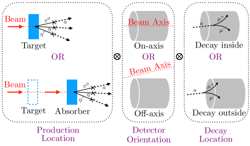
Figure 1: In this schematic diagram, the three columns show possible production locations, beam directions with respect to the detector, and decay locations. The axions can be produced from the beam at the target or at the absorber. The detector, shown by the gray cylinder, may be on- or off-axis from the beam. Lastly, the axion may decay inside or before entering the detector.

This work is organized as follows. In Sec. II we review the axion quality problem and motivate how heavy QCD axions can improve it. Then we describe the couplings of the heavy QCD axion to the SM using an effective field theory (EFT) framework. After describing the various decay modes of the axion, in Sec. III we study the details of axion production in various neutrino and beam dump experiments. With these results at hand, we derive the projected reach that SBND, ICARUS, DUNE, FASER 2, and SHiP may be able to achieve, and then summarize the existing constraints on the axion parameter space coming mostly from rare meson decays. In Sec. IV we describe examples of UV completions that can give rise to the axion EFT under consideration. We conclude in Sec. V.

II Heavy QCD Axion EFT

We start our general analysis with an EFT approach, and we will present examples of UV realization in Sec. IV. After reviewing the role the heavy axions play in the context of the quality problem, we describe the EFT and summarize the decay modes of the axion.

II.1 Axion Quality Problem and Heavy QCD Axions

As alluded to in the introduction, the axion quality problem is that $U(1)_{\rm PQ}$ breaking contributions could generally arise from gravitational corrections. Such corrections can give rise to new CP non-conserving minima, and as the axion dynamically relaxes to such a minimum, the strong CP problem reappears. To be quantitative, we first consider the case of the standard QCD axion which couples to QCD as

$$\mathcal{L}\supset\frac{\alpha_{s}}{8\pi}\left(\frac{a}{f_{a}}+\bar{\theta}\right)G_{\mu\nu}^{a}\tilde{G}^{a,\mu\nu}.$$ (1)

Upon QCD confinement this gives rise to an axion potential DiVecchia:1980yfw ; GrillidiCortona:2015jxo

$$V_{\rm QCD}(a)=-m_{\pi}^{2}f_{\pi}^{2}\sqrt{1-\frac{4m_{u}m_{d}}{(m_{u}+m_{d})^{2}}\sin^{2}\left(\frac{a}{2f_{a}}+\frac{\bar{\theta}}{2}\right)}.$$ (2)

Here $m_{\pi},f_{\pi}$ are the pion mass and decay constant, and $m_{u},m_{d}$ are up and down quark masses, respectively. This determines the QCD axion mass to be,

$$m^{\rm QCD}_{a}\approx\frac{\sqrt{m_{u}m_{d}}}{m_{u}+m_{d}}\frac{m_{\pi}f_{\pi}}{f_{a}}\approx 5.7\left(\frac{10^{9}~{}{\rm GeV}}{f_{a}}\right)~{}{\rm meV}.$$ (3)

To see how the axion quality problem arises in this context, consider the case where the axion is a pseudo-Nambu-Goldstone boson of a spontaneously broken $U(1)_{\rm PQ}$ symmetry. The axion can then be written as the phase residing in the PQ scalar, $\Phi\sim f_{a}e^{ia/f_{a}}$. Gravitational violation of this global PQ symmetry effects would then imply Lagrangian terms like

$$\frac{\Phi^{n}}{M_{\rm Pl}^{n-4}}\supset\frac{f_{a}^{n}}{M_{\rm Pl}^{n-4}}\cos\left(\frac{na}{f_{a}}+\varphi_{n}\right)$$ (4)

would be present, and they would give rise to extra contributions to the axion potential. Now a variety of astrophysical constraints on the QCD axion imply $f_{a}\gtrsim 10^{8}$ GeV Ellis:1987pk ; Raffelt:1987yt ; Turner:1987by ; Mayle:1987as ; Raffelt:2006cw ; Payez:2014xsa ; Chang:2018rso ; Carenza:2019pxu ; Bar:2019ifz ; Buschmann:2021juv . Given the light axion mass dictated by Eq. (3), we then see that unless we forbid all higher dimensional operators up to $n=8$, the gravitational contributions would move the axion away from the CP conserving minima, spoiling the solution to the strong CP problem.

To contrast this scenario, we now focus on heavy QCD axions. As an example for this class of models, consider the scenario where the axion couples to a dark gauge group that confines at a scale $\Lambda_{D}\gg\Lambda_{\rm QCD}$. As a result, the axion obtains a potential of the type,

$$V_{D}(a)\simeq\Lambda_{D}^{4}\cos\left(\frac{a}{f_{a}}+\delta\right).$$ (5)

Due to the fact that $\Lambda_{D}\gg\Lambda_{\rm QCD}$, the dynamical relaxation of the axion is mostly dictated by this potential, rather than Eq. (2). Because of the structure of the theory, such as the presence of an additional $\mathbb{Z}_{2}$ mirror symmetry Rubakov:1997vp ; Berezhiani:2000gh ; Hook:2014cda ; Fukuda:2015ana ; Dimopoulos:2016lvn ; Hook:2019qoh or embedding of $SU(3)_{c}$ into larger gauge groups Dimopoulos:1979pp ; Gherghetta:2016fhp ; Gaillard:2018xgk ; Agrawal:2017evu ; Gherghetta:2020ofz ; Valenti:2022tsc , the axion can still solve the strong CP problem while being heavier than the QCD axion.

Now the situation is quite improved from the perspective of the quality problem. Through Eq. (5), the axion mass is given by $m_{a}\simeq\Lambda_{D}^{2}/f_{a}$ and is much larger than that from Eq. (2) for identical values of $f_{a}$. Existing constraints on such heavier axions can be much weaker compared to the QCD axion. In particular, as the axion mass becomes larger than ${\cal O}(100)$ MeV, the astrophysical and cosmological constraints can weaken and parameter space with $f_{a}\ll 10^{8}$ GeV is then allowed by the current set of constraints. Consequently, these smaller values of $f_{a}$ reduce the strength of the gravitational contributions seen in Eq. (4) and correspondingly, the axion potential becomes robust against such corrections. In particular, for some of the $m_{a}$ and $f_{a}$ values we consider in the rest of this work, one needs to forbid only the dimension-5 term in Eq. (4). This, therefore, reduces the severity of the quality problem.

II.2 Lagrangian and Low Energy Effective Theory

Generic ALPs can couple to the SM in a variety of ways. However, the heavy QCD axions that we focus on in this work have a defining coupling to QCD since that is essential for solving the strong CP problem. At the same time, motivated by gauge coupling unification, we focus on a class of EFTs where axions also couple to $SU(2)_{L}$ and $U(1)_{Y}$ gauge bosons. Therefore, we consider the following gauge sector coupling,

$$\mathcal{L}_{\rm gauge}=c_{3}\frac{\alpha_{s}}{8\pi f_{a}}aG\tilde{G}+c_{2}\frac{\alpha_{2}}{8\pi f_{a}}aW\tilde{W}+c_{1}\frac{\alpha_{1}}{8\pi f_{a}}aB\tilde{B}.$$ (6)

This particular set of couplings also appears in the context of KSVZ axions. In the following, we will set $c_{3}=c_{2}=c_{1}=1$. Along with the gauge coupling, axions can also couple to fermions. In the present work, we consider only flavor-diagonal lepton couplings of the axion. The motivation is two-fold. First, since the axion does not couple to quarks and also does not give rise to flavor-changing processes at the tree level, we can focus on a parameter space that is not strongly constrained by existing searches, such as those of rare meson decays (see, e.g., Goudzovski:2022vbt for a recent summary). This then lets us focus on a complementary part of the parameter space. Second, given the leptonic coupling of the axion, it can dominantly decay into a pair of muons. As we will discuss later, the resulting dimuon signature can be a powerful discovery channel for GeV-scale axions. Therefore, we consider a lepton sector coupling,

$$\mathcal{L}_{\rm lepton}=\sum_{\ell=e,\mu,\tau}c_{\ell}\frac{\partial_{\mu}a}{2f_{a}}\bar{\ell}\gamma^{\mu}\gamma_{5}\ell.$$ (7)

As we will show in Sec. IV, such a scenario can naturally arise in UV complete models. To summarize, the axion EFT in our scenario is given by,

$$\mathcal{L}_{\rm axion}=\frac{1}{2}(\partial_{\mu}a)^{2}-\frac{1}{2}m_{a}^{2}a^{2}+\mathcal{L}_{\rm gauge}+\mathcal{L}_{\rm lepton},$$ (8)

at some UV scale $\Lambda\sim 4\pi f_{a}$. Below $\Lambda$, various other operators are introduced via renormalization group (RG) evolution. We follow Refs. Bauer:2021wjo ; Bauer:2021mvw to account for the RG evolution and compute the axion couplings below the GeV scale.

II.3 Axion Decay

Given the EFT in Eq. (6) and Eq. (7), the axion dominantly decays into three classes of final states: ($a$) diphotons, ($b$) dimuons, and ($c$) hadrons. We discuss each of them briefly now.

Photons:

The width for an axion decaying into two photons is given by,

$$\Gamma_{a\rightarrow\gamma\gamma}=\frac{\alpha^{2}|c_{\gamma}|^{2}m_{a}^{3}}{256\pi^{3}f_{a}^{2}}.$$ (9)

Here $c_{\gamma}$ is determined in terms of the EFT coefficients appearing in Eqs. (6) and (7) as Bauer:2017ris ; Aloni:2018vki ; Georgi:1986df ,

$$c_{\gamma} =c_{3}\left(-1.92+\frac{1}{3}\frac{m_{a}^{2}}{m_{a}^{2}-m_{\pi}^{2}}+\frac{8}{9}\frac{m_{a}^{2}-\frac{4}{9}m_{\pi}^{2}}{m_{a}^{2}-m_{\eta}^{2}}+\frac{7}{9}\frac{m_{a}^{2}-\frac{16}{9}m_{\pi}^{2}}{m_{a}^{2}-m_{\eta^{\prime}}^{2}}\right)+\frac{5}{3}c_{1}+c_{2}+2\sum_{\ell=e,\mu,\tau}c_{\ell}B(4m_{\ell}^{2}/m_{a}^{2}),$$ (10)

and $\alpha$ the fine-structure constant. Here $B(x)=1-xf(x)^{2}$ and

$$f(x)=\begin{cases}\sin^{-1}\left(\frac{1}{\sqrt{x}}\right)&\quad\text{if }x\geq 1\\ \frac{\pi}{2}+\frac{i}{2}\log\left(\frac{1+\sqrt{1-x}}{1-\sqrt{1-x}}\right)&\quad\text{if }x<1\end{cases}\,.$$ (11)

For our choices of $c_{i}$, the diphoton mode dominates below the dimuon threshold.

Muons:

The axion width into muons is given by,

$$\Gamma_{a\rightarrow\mu\mu}=\frac{c^{2}_{\ell}m_{a}m_{\mu}^{2}}{8\pi f_{a}^{2}}\sqrt{1-\frac{4m_{\mu}^{2}}{m_{a}^{2}}}.$$ (12)

Here and in the following, we will use $c_{\ell}$ to denote all the lepton couplings, i.e., assuming them to be flavor-diagonal. Soon above the kinematic threshold, the muon decay modes dominate over the diphoton channel, except in regions where the axion resonantly mixes with SM pseudoscalar mesons.

Hadrons:

Below the QCD scale, the axion also couples to various hadrons, thanks to the axion-gluon coupling. For $m_{a}\lesssim$ GeV, the dominant decay channels are into $\pi\pi\pi,\eta\pi\pi,\pi\pi\gamma$. We use the results of Ref. Aloni:2018vki to take these decays into account. The relative importance of these modes compared to the dimuon mode depends on the values of $c_{\ell}$, and we consider two benchmark scenarios $c_{\ell}=1/36$ and $c_{\ell}=1/100$ to illustrate the differences. As will be discussed in more detail in Sec. IV, the coefficient $c_{\ell}$ roughly corresponds to a mixing angle squared $\theta_{\rm mix}^{2}$ in one UV completion that we will focus on. Thus the choices $c_{\ell}=1/36,1/100$ originate from $\theta_{\rm mix}\simeq 1/6,1/10$, respectively.

The relative contributions to the decay width of the photon mode (dotted), muon mode (dashed), and hadronic modes (dot-dashed) for the two benchmark choices are shown in Fig. 2.

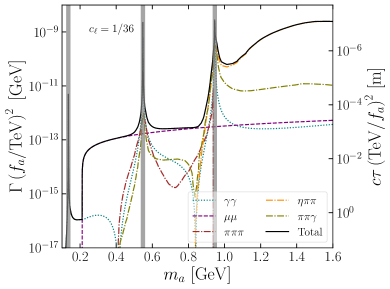
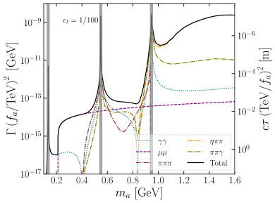
Figure 2: The relative contributions of various decay channels to the total width of the axion for $c_{\ell}=1/36$ (left) and $c_{\ell}=1/100$ (right). For $2m_{\mu}<m_{a}\lesssim 0.8$ GeV, the axion dominantly decays into a pair of muons.

III Beam Dump Considerations

In this section, we discuss some of the details of axion production in a beam dump environment in the presence of a gluon coupling. We consider several neutrino experiments: ArgoNeuT Anderson:2012vc , SBND MicroBooNE:2015bmn , ICARUS MicroBooNE:2015bmn and DUNE DUNE:2018hrq for which axions are produced when a proton beam hits a stationary target (or an absorber placed downstream). While a similar setup is also true for SHiP SHiP:2015vad , we also study the discovery capabilities of FASER 2 for which axions would get produced in 14 TeV $pp$ collisions at the LHC. The axions produced in the forward direction can then travel to the FASER 2 detector.

III.1 Production

The theory of axion production in the presence of gluon couplings is an active area of research. Along with axion production in meson mixing or gluon fusion for higher masses, axion production in proton bremsstrahlung can also be an important contribution. For scalars, this was computed in Refs. Boiarska:2019jym ; Foroughi-Abari:2021zbm ; SplittingAxions , while for the case of pseudoscalars, there are subtleties. These subtleties SplittingAxions include the axion flux dependence on the exact form of quasi-real approximation, the interference between initial state radiation and final state radiation, the comparison of the proton bremsstrahlung calculation and the hadronization contribution in the regime of concern, as well as the exact order of mass expansion and momentum expansion. Some of these subtitles arise because the phase space of interest involves scales comparable to the axion mass and the CP nature of the axion-fermion coupling, and because the formalism itself is only an approximation heavily dependent on the matching procedure and scheme at a fixed order. Given all these subtleties, we still approximate the axion production rate by the SM pseudoscalar production rate multiplied by the square of the axion-pseudoscalar mixing angle, as is widely done in the current literature. Since these mixing angles depend on the axion-quark coupling, a field rotation-dependent quantity Blinov:2021say ; SplittingAxions , such an approximation needs to be improved. Furthermore, this approximation also heavily relies on the SM QCD production of mesons, and involves an unphysical, ad hoc assignment of the SM meson four momentum to the axion four momentum. This approximation also ignores the interference effects from different axion-meson contributions to the production. Hence, future improvement in the axion flux prediction would be highly desirable. With these caveats in mind, we now estimate the flux of axions produced only via meson mixing.

The mixing production is primarily driven by axion mixing with the Standard Model mesons $\pi$, $\eta$, and $\eta^{\prime}$. In a convenient choice of basis, the corresponding mixing angles are given by Bauer:2017ris ; Ertas:2020xcc ; Kelly:2020dda ,

$$\theta_{a\pi} =\dfrac{1}{6}\dfrac{f_{\pi}}{f_{a}}\dfrac{m_{a}^{2}}{m_{a}^{2}-m_{\pi}^{2}},\hskip 28.45274pt\theta_{a\eta} =\dfrac{1}{\sqrt{6}}\dfrac{f_{\pi}}{f_{a}}\dfrac{m_{a}^{2}-4m_{\pi}^{2}/9}{m_{a}^{2}-m_{\eta}^{2}},\hskip 28.45274pt\theta_{a\eta^{\prime}} =\dfrac{1}{2\sqrt{3}}\dfrac{f_{\pi}}{f_{a}}\dfrac{m_{a}^{2}-16m_{\pi}^{2}/9}{m_{a}^{2}-m_{\eta^{\prime}}^{2}}.$$ (13)

Using Pythia8 Bierlich:2022pfr ; Sjostrand:2014zea , we determine how many mesons are produced per proton collision by turning on the “SoftQCD:all = on” option. This is dependent on the energy of the incoming beam. We show the results below for the 8 GeV Booster Neutrino Beam (BNB) Stancu:2001cpa , 120 GeV NuMI proton beam, 400 GeV SPS beam and finally 14 TeV LHC,

$$N_{\rm axions}=N_{\rm POT}\times\begin{cases}0.82|\theta_{a\pi}|^{2}+0.072|\theta_{a\eta}|^{2}+0.0038|\theta_{a\eta^{\prime}}|^{2}~{}~{}{\rm for~{}}8~{}{\rm GeV~{}BNB}\\ 2.9|\theta_{a\pi}|^{2}+0.33|\theta_{a\eta}|^{2}+0.034|\theta_{a\eta^{\prime}}|^{2}~{}~{}{\rm for~{}}120~{}{\rm GeV~{}NuMI~{}beam}\\ 4.0|\theta_{a\pi}|^{2}+0.46|\theta_{a\eta}|^{2}+0.049|\theta_{a\eta^{\prime}}|^{2}~{}~{}{\rm for~{}}400~{}{\rm GeV~{}SPS~{}beam}\\ 33|\theta_{a\pi}|^{2}+3.8|\theta_{a\eta}|^{2}+0.48|\theta_{a\eta^{\prime}}|^{2}~{}~{}{\rm for~{}}14~{}{\rm TeV~{}LHC}\end{cases}\,,$$ (14)

where $N_{\rm POT}$ is the number of protons on target (POT). Following their production, axions travel a macroscopic distance to reach the detector and can subsequently give a displaced decay signal.

III.2 Detection

The produced axions will travel to the detector and decay to various final states. We will show prospects for SBND, ICARUS, DUNE, SHiP, and FASER 2 on detecting these decays. We specifically search for the signatures associated with the dimuon final states. LArTPCs identify muons by the profile of the energy loss per unit track length $dE/dx$, as a function of the residual range, defined as the distance to the particle’s stopping point. The pair of muons will leave either one or two distinct minimally ionizing tracks depending on the opening angles and the detector’s angular resolution. The SHiP experiment has a dedicated muon detector composed of three layers of scintillators with iron absorbers in between and is located at the most downstream location Tosi:2019xok , before which the hadron calorimeter would stop most of the hadrons. The FASER 2 experiment utilizes an emulsion detector Nakamura:2005xov with silver bromide crystals dispersed in gelatin media, and muons are identified by the track lengths FASER:2019dxq . Among these detectors, the magnetic field in DUNE, SHiP, FASER 2, and potentially also ICAURS Antonello:2013ypa , would play an important role in increasing the separation between the two muon tracks. Correspondingly, the invariant mass of the dimuon system can serve as a useful handle in background mitigation.

In Table 1, we summarize the detector specifications. Here $E_{p}$ refers to the energy of the proton beam on target, $N_{\rm POT}$ is the total number of protons on target, $d$ is the distance from the target to the detector, $L$ is the length of the detector along the beam direction, while $w\times h$ is the width and height of each detector.

In deriving the experimental prospects, we will approximate any rectangular cross section by a disk with radius shown as $r_{\rm eff}$, while FASER 2 has a circular cross section $r=1$ m. DUNE near detector (ND) complex consists of a gaseous argon and a liquid argon time projection chamber along the beam direction; both chambers have length 5 m, while the gaseous (liquid) argon chamber has a circular (rectangular) cross section of (effective) radius ($r_{\rm eff}=2.6$ m) $r=2.5$ m. ICARUS has two modules of the same size next to each other; therefore, the effective cross section is multiplied by 2 in the table. For ICARUS, we will show the results for the protons from both the off-axis, 120 GeV NuMI beam and the default on-axis, 8 GeV BNB since the former has a better prospect for our search. For SBND we will show only the results for 8 GeV BNB, which may achieve a better reach compared to the NuMI beam. While we will not show the results for MicroBooNE explicitly, we have checked that it performs similarly to the other SBN experiments in our analysis.

Experiments	$E_{p}$ (GeV)	$N_{\rm POT}$	$d$ (m)	$L$ (m)	$w\times h$ (m$\times$m)
DUNE DUNE:2020ypp ; DUNE:2020fgq	120	$1.47\times 10^{22}$	574	5 + 5	$7\times 3$  ($r_{\rm eff}=$ 2.6 m)
SBND Bonesini:2022pwy $\begin{dcases}{\rm BNB}\\ {\rm NuMI}\end{dcases}$	8 120	$6.6\times 10^{20}$ $3\times 10^{21}$	110 410	5	$4\times 4$  ($r_{\rm eff}=$ 2.3 m)
MicroBooNE MicroBooNE:2017tkp ; Bonesini:2022pwy $\begin{dcases}{\rm BNB}\\ {\rm NuMI}\end{dcases}$	8 120	$1.32\times 10^{21}$ $3\times 10^{21}$	470 685	10.4	$2.6\times 2.3$  ($r_{\rm eff}=$ 1.4 m)
ICARUS Bonesini:2022pwy $\begin{dcases}{\rm BNB}\\ {\rm NuMI}\end{dcases}$	8 120	$6.6\times 10^{20}$ $2.5\times 10^{21}$	600 790	19.9	$(3.9\times 3.6)\times 2$  ($r_{\rm eff}=$ 2.1 m)
SHiP SHiP:2021nfo	400	$2\times 10^{20}$	70	50	$5\times 10$  ($r_{\rm eff}=$ 4.0 m)
FASER 2 FASER:2019aik ; Feng:2022inv	14000	$1.1\times 10^{16}$ (LHC Run 3) $2.2\times 10^{17}$ (HL-LHC)	480	5	$r=1$ m

Table 1: Detector specifications for various experiments. For DUNE, we have combined the lengths of the gaseous multi-purpose detector (5 m) and LArTPC (5 m). SBND, MicroBooNE, and ICARUS can serve as useful facilities as off-axis detectors with respect to the NuMI beam, along with the default on-axis BNB. Therefore, we record the locations and geometries for both beams.

Using the above details for axion production and detector dimensions, we can compute the energy distributions of axions both at the production point and at the detector. In Fig. 3 we show these results for the DUNE ND (left) and FASER 2 (right). For both the panels, we see that the spectrum at production peaked at low energies as expected, with the axions at FASER 2 being more energetic than at DUNE ND due to larger incoming beam energies. The axions that decay inside the detector need sufficient energy so that their lab-frame lifetime is long enough to reach the detector. We see this explicitly in Fig. 3—for smaller $f_{a}$, the rest-frame lifetime is shorter, and correspondingly, the axions need to be more energetic with a large Lorentz factor $\gamma$. This is why the distributions move towards higher energies as $f_{a}$ decreases.

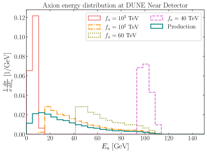
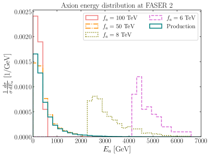
Figure 3: The differential energy distribution of the axions at production (in teal) and at the detectors (for various values of $f_{a}$ in other colors and line styles). We fix $c_{\ell}=1/36$ and $m_{a}=0.8$ GeV.

III.3 Enhanced Effective Detector Length

The axion to dimuon decay channel not only has the feature of being clean and highly identifiable but also can allow for an enhancement in the decay volume. These high-energy muons can penetrate air and rocks without significant loss in energy and deflection. In this section, we take the geometry of DUNE ND as an example and show the interplay between enhanced decay volume and signal efficiency, with their dependence on the axion mass and energy.

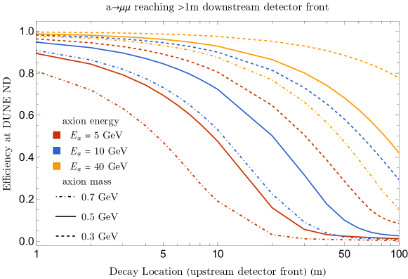
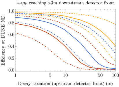
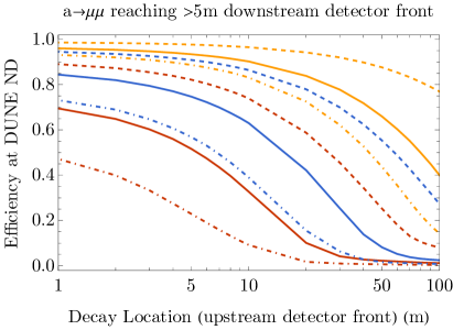
Figure 4: The signal axion decay geometrical acceptance, as a function of decay location before the front panel of the detector (upstream) for various axion masses and energies. Depending on the background rejection requirement and the actual performance of the detector, one might require a certain track length for the dimuon signals. As most of the axions are boosted, the decay is forward, so most of the signal will penetrate the whole detector. We show the acceptance fraction by requiring both the muons to arrive at least 1 meter (upper panel), which is equivalent to a track length of more than 1 meter, 3 meters (lower left panel), and 5 meters (lower right panel). The red, blue, and yellow curves correspond to axion energy of 5, 10, and 40 GeV, respectively. The dashed, solid, and dot-dashed curves correspond to axion masses of 0.3, 0.5, and 0.7 GeV.

For axion decay before the detector, several physics effects must be considered. One is geometric acceptance: the further the decay location away from the detector, the lower the geometric acceptance. This is because the geometric acceptance would be proportional to the area divided by the distance. Thanks to the boosted kinematics of the beam dump experiments and the forward physics at colliders, the penalty is reduced by the fact that axions are already focused towards the target after getting boosted from an isotropic distribution in their rest frame. The second factor one needs to consider is the change in the signal-to-background ratio. Because the decay location is outside the detector, the vertex cannot be directly reconstructed within the detector volume and hence typically would have larger uncertainties in its location. In this sense, other muons, such as those generated through various nuclear interactions of the beam remnants can contribute to the background. To avoid complexities, we conservatively require both of the muons from the axion decay to arrive at the detector. The third factor is that the muons lose energy and slightly change their momentum direction while passing through matter. One can estimate the typical energy loss and deflection for the minimally ionizing muons and see that for typical high-energy muons from the axion decays with tens of GeV of energies passing through 100 meters of dirt, these effects are small ParticleDataGroup:2020ssz . Again being conservative, we do not consider the decay location more than 100 meters before the detector front panel.

Each experiment is conducted in a different setup; the amount of shielding varies, and the material before the detector varies (they can be air, dirt, or even another detector). However, the effective gain of the decay volume in the muon mode is a common feature. To concretely demonstrate this effective volume increase, we use the DUNE ND setup and simulate axion decay acceptance as a function of axion mass, energy, and muon track reconstruction requirement (track length) and show them in Fig. 4. As expected, the acceptance decreases as one increases the separation between the axion decay location and detector location. Still, for most signals, one can achieve more than 50% acceptance even for decays occurring 30 meters before the detector. We can see that decays from heavier axions have lower acceptance for fixed axion energy. These observations lead to our discussion and presentation of projected sensitivities in the following subsection.

III.4 Results

In this subsection, we show the results of our projection study and our re-interpreted limits from existing experiments on heavy axions in the mass range under consideration.

III.4.1 Future Projections

For future projections, we analyze several neutrino experiments: SBND, ICARUS, and DUNE, as well as collider experiments searching for long-lived particles: FASER 2 and SHiP. The main idea is that the axion production would happen at the beam dump or at the primary interaction point. Subsequently, the axion would travel to the decay volume of the detector and dominantly decay into a pair of muons. For our final projections, we will assume a 90% reconstruction efficiency of the muons along with a negligible background.

While an actual $\mu^{+}\mu^{-}$ background would be reducible, in LArTPCs charged pions can mimic muons, giving rise to background events. In Ref. ArgoNeuT:2022mrm , such backgrounds were mitigated via matching track information in ArgoNeuT with MINOS near detector, along with restrictions on track length. This latter restriction helped since pions tend to produce shorter tracks compared to muons at energies relevant to that search. A similar approach could be taken up at DUNE with the help of its multipurpose near detector to mitigate such backgrounds. Furthermore, in the case of magnetized detectors, the invariant mass would serve as a powerful discriminator as well. Dedicated simulations by experimental collaborations would be necessary to settle these aspects conclusively. Keeping this in mind, we show results for signal flux at various detectors in Fig. 5, for several choices of $m_{a}$. This can then be used to obtain more conservative projections for a search with non-negligible number of background events.

To this end, we first compute the number of signal events produced at the detectors of interest. For some benchmark choices of $m_{a}$ we show the results for SBND, ICARUS, DUNE ND, and FASER 2 in Fig. 5 as a function of $f_{a}$. The number of axions reaching the detector can be roughly estimated as

$$N_{\rm axions}\sim N_{\rm POT}\times N_{\rm mesons}\times\left(\frac{f_{\pi}}{f_{a}}\right)^{2}\times{\rm BR}\times{\rm acceptance}\times\left(e^{-\frac{d}{\gamma\beta c\tau}}-e^{-\frac{d+L}{\gamma\beta c\tau}}\right).$$ (15)

Here $N_{\rm mesons}$ is the number of mesons produced per collision with each meson mixing into axions with a probability $(f_{\pi}/f_{a})^{2}$, away from any resonance. A fraction, denoted by ‘acceptance’, of the produced axions are in the direction of detector which decay inside it with a probability $\left(e^{-\frac{d}{\gamma\beta c\tau}}-e^{-\frac{d+L}{\gamma\beta c\tau}}\right)$ into dimuons with a branching ratio ‘BR’. Here $\tau$ is the rest-frame lifetime of the axions, $\gamma$ is the Lorentz factor, and $\beta$ is the dimensionless velocity. Based on Eq. (15), we see for very small values of $f_{a}$, although more axions are produced via the mixing factor $(f_{\pi}/f_{a})^{2}$, the axions are too short-lived to reach the detector, $\gamma\beta c\tau\ll d$. As a result, the number of signal events gets exponentially suppressed. As $\gamma\beta c\tau\sim d$, the signal turns on, and eventually for large enough $f_{a}$, $\gamma\beta c\tau\gg d$. In this large lifetime regime, the signal decreases as $N_{\rm axions}\propto L/f_{a}^{4}$, as can be seen via Fig. 5 and Eq. (15).

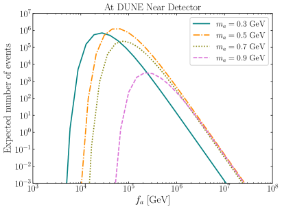
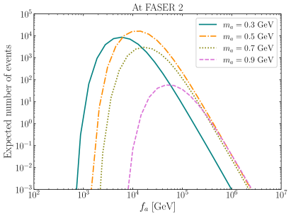
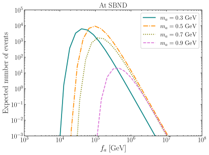
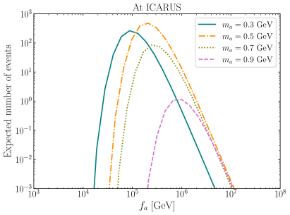
Figure 5: The expected number of events at DUNE ND, FASER 2, SBND, and ICARUS in which the axion decays into dimuons within the detector, as a function of the decay constant $f_{a}$. Different curves are for different axion masses $m_{a}$ as labeled. We fix $c_{\ell}=1/36$.

To derive the maximal sensitivity, we show the reach curves on the axion parameter space assuming 3 signal events for various experiments in Fig. 6. Similar reach curves requiring a larger number of signal events, in the event of non-negligible backgrounds, can be obtained from Fig. 5. We see that among the neutrino experiments, DUNE ND would be able to provide the strongest probe, thanks to its large $N_{\rm POT}$ and decay volume. However, overall, SHiP would provide the best sensitivity. This is due to its larger beam energy, proximity to the target, as well as larger decay volume. While ICARUS with its on-axis BNB would constrain novel parameter space, it can operate even more powerfully via the off-axis NuMI beam due to a larger beam energy which is not completely compensated by a larger distance. This is labeled as ICARUS* in Fig. 6. In the context of DUNE ND, we also show the result of including a distance of 30 m before the front detector panel as part of the decay volume, as discussed in Sec III.3. This is labeled as ‘DUNE⁺’ in Fig. 6. While in the small lifetime, i.e., small $f_{a}$ regime, the gain is not significant, in the large lifetime regime the sensitivity to $f_{a}$ increases as $\propto L^{1/4}$, as expected from Eq. (15) above.

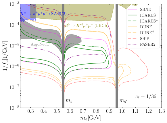
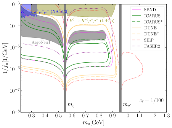
Figure 6: Constraints (shaded-regions) and projections (curves) for $c_{\ell}=1/36$ (upper panel) and $c_{\ell}=1/100$ (lower panel). The curve labeled ${\rm DUNE}^{+}$ denotes a scenario in which the axion can decay up to 30 m before the DUNE ND. The high-energy muons produced via these decays can still reach the detector. The curve labeled ${\rm ICARUS}^{*}$ is for the reach ICARUS would have through the off-axis NuMI beam. See text for more details.

III.4.2 Existing Constraints

The strongest constraints on the parameter space come from some of the rare meson decay searches which we now describe.

NA48/2 $K^{\pm}\rightarrow\pi\mu\mu$ search NA482:2016sfh :

In the presence of the axion-gluon coupling, flavor changing couplings get induced at loop-level. For example, an axion-gluon coupling induces flavor-diagonal couplings to quarks, which then can give rise to flavor-changing processes through the CKM couplings. As a result, processes such as $K\rightarrow\pi a$ with $a$ decaying into $\mu^{+}\mu^{-}$ can take place. We use the results of Refs. Bauer:2021mvw ; Bauer:2021wjo to first compute $K\rightarrow\pi a$ amplitude. Subsequently, we use the results of Ref. NA482:2016sfh , where upper limits on $\text{BR}(K^{\pm}\rightarrow\pi^{\pm}X(\mu^{+}\mu^{-}))$ were derived for various lifetimes of an unstable resonance $X$, to arrive at the constraints shown in blue in Fig. 6.

LHCb $B^{0}\rightarrow K^{*0}\mu\mu$ search LHCb:2015nkv :

Above the kinematic threshold of $(m_{K}-m_{\pi})$, rare $B$ decays become the dominant probe of our scenario. Similar as above, we use the results of Ref. Bauer:2021wjo to first compute the rate for $B^{0}\rightarrow K^{*0}a$ amplitude, and then use the upper limits on $\text{BR}(B^{0}\rightarrow K^{*0}X(\mu^{+}\mu^{-}))$ from Ref. LHCb:2015nkv for different lifetimes of $X$, to arrive at the constraints shown in olive in Fig. 6. A similar bound was also derived in Ref. Freytsis:2009ct using rare $B$-decays for DFSZ-style axion couplings.

Other searches:

Searches for $K\rightarrow\pi+{\rm inv.}$ NA62:2021zjw are also applicable when axion decays invisibly due to its large lifetime. For our scenario, however, this constraint is applicable only for $m_{a}<2m_{\mu}$, since otherwise, axion would promptly decay into dimuons. Searches for exotic $B$ decays such as $B\rightarrow K\eta_{X}(\eta\pi\pi)$ BaBar:2008rth where $\eta_{X}$ is one of the excited states of $\eta,\eta^{\prime}$ mesons, can also be used to constrain processes such as $B\rightarrow Ka(\eta\pi\pi)$ Chakraborty:2021wda . These are mostly subdominant in our parameter space and are not shown in Fig. 6. A recent CMS search CMS:2021sch for long-lived particles decaying into muon pairs can also be relevant in a similar parameter space covered by the LHCb search for $B^{0}\rightarrow K^{*0}\mu^{+}\mu^{-}$. This would require a dedicated recasting as appropriate for gluon-coupled axions, such as production simulation using gluon fusion and applying their kinematic selection criteria, and we do not carry that out here.

Along with these constraints from rare meson decay searches, we show in the gray-shaded region the recent ArgoNeuT constraint ArgoNeuT:2022mrm that the ArgoNeuT collaboration and the present authors obtained. In this case, following their production in the beam dump, the axions would travel to the ArgoNeuT detector and dominantly decay into a pair of muons. We consider only the axions produced by the protons that reach the hadron absorber located 318 m upstream of ArgoNeuT, which is about $13\%$ of the total $N_{\rm POT}$ collected during its run. The axions produced by the rest of the protons that hit the target located 1033 m upstream of the ArgoNeuT detector give a subdominant sensitivity compared to the absorber-produced axions we consider. By searching for such muon pairs, with information from both the ArgoNeuT and MINOS near detector, we could place new constraints as shown in Fig. 6.

IV Examples of UV Completion

In this section, we describe some examples of UV models to show how the axion couplings in Eqs. (6) and (7) can arise. We pay particular attention to models that generate the small axion-lepton couplings, compared to gauge boson couplings, considered in the previous section.

A particularly simple possibility is where $c_{\ell}$ is zero at tree-level but radiatively induced by the coupling of the axion with the gauge bosons. The contributions to the axion-lepton coupling from one-loop radiative corrections with $c_{1},c_{2}$, and $c_{3}$ are given in Ref. Bauer:2020jbp for $f_{a}=1~{}\mathrm{TeV}$ as

$$c_{\ell}\simeq\left(0.05c_{1}+0.22c_{2}+0.37c_{3}\right)\times 10^{-3}.$$ (16)

The coefficients depend on the renormalization scale but may only increase by a factor of $\mathcal{O}(3)$ for $f_{a}\simeq\mathcal{O}(10^{7})~{}\mathrm{GeV}$. Therefore, to obtain $c_{\ell}\simeq 1/100$ that is of interest in the previous section, one needs $c_{1,2}=\mathcal{O}(10)$, and therefore a small hierarchy from $c_{3}$ is necessary since $c_{3}$ is conventionally normalized to unity for QCD axions. This is the case if there are more heavy fermions charged under $U(1)_{Y}$ and $SU(2)_{L}$ that generate $c_{1,2}$ than those under $SU(3)_{c}$ for $c_{3}$. Some examples of enhancing certain axion couplings this way include the Kim-Nilles-Peloso mechanism Kim:2004rp and the clockwork axion Kaplan:2015fuy .

To generate an axion-lepton coupling larger than the one-loop contributions, we now describe a model based on Ref. Buen-Abad:2021fwq , where the coupling arises from the mixing of SM leptons with new heavy fermions. The model has a SM singlet PQ scalar $\Phi$, heavy vector-like leptons $L_{i},L^{c}_{i},E_{i},E^{c}_{i}$, and heavy vector-like quarks $Q,Q^{c}$. The index $i=1,2,3$ runs over the SM flavor indices. The charge assignments for the left-handed fields are as given in Table 2.

Field	$SU(3)_{c}$	$SU(2)_{L}$	$U(1)_{Y}$	$U(1)_{\rm PQ}$
$L_{i}$	1	$\Box$	+1/2	$-$1
$L^{c}_{i}$	1	$\Box$	$-$1/2	+1
$E_{i}$	1	1	$-$1	$-$1
$E^{c}_{i}$	1	1	+1	+1
$Q$	$\Box$	$\Box$	$+1/\sqrt{2}$	$-$1/2
$Q^{c}$	$\bar{\Box}$	$\Box$	$-1/\sqrt{2}$	$-$1/2
$\Phi$	1	1	0	+1
$l_{i}$	1	$\Box$	$-$1/2	0
$e_{i}$	1	1	+1	0

Table 2: Charge assignment for the UV model

With this choice, the Lagrangian can be written as

$$\mathcal{L}\supset y_{L_{i}}L_{i}l_{i}\Phi+y_{E_{i}}E_{i}e_{i}\Phi+y_{Q}QQ^{c}\Phi+M_{L}L_{i}L^{c}_{i}+M_{E}E_{i}E_{i}^{c}+\rm{h.c.}.$$ (17)

Here $M_{L}$ and $M_{E}$ are vector-like masses for heavy leptons. The PQ scalar $\Phi$ has a potential suitable for symmetry breaking and we parametrize the axion as $\Phi=((f_{a}+\rho)/\sqrt{2})e^{ia/f_{a}}$. For $M_{L},M_{E}\gg f_{a}$, we can integrate out the heavy leptons at tree level to obtain their equations of motion,

$$L^{c}_{i}=-\frac{y_{L_{i}}}{M_{L}}l_{i}\Phi,~{}~{}E^{c}_{i}=-\frac{y_{E_{i}}}{M_{E}}e_{i}\Phi.$$ (18)

Substituting this into the kinetic term for $L^{c}_{i}$, we get

$$iL_{i}^{c\dagger}\bar{\sigma}^{\mu}\partial_{\mu}L^{c}_{i}\rightarrow i\dfrac{|y_{L_{i}}|^{2}}{M_{L}^{2}}l_{i}^{\dagger}\Phi^{\dagger}\bar{\sigma}_{\mu}\partial_{\mu}(l_{i}\Phi)\supset i\dfrac{|y_{L_{i}}|^{2}}{M_{L}^{2}}l_{i}^{\dagger}\Phi^{\dagger}\bar{\sigma}_{\mu}l_{i}\partial_{\mu}\Phi+\cdots.$$ (19)

Here in the last relation, we have dropped a correction to the SM fermion kinetic term. We can carry out the above steps for $e_{i}$ as well. Consequently, in the EFT below $M_{L},M_{E}$, we have

$$\mathcal{L}\supset i\dfrac{|y_{L_{i}}|^{2}}{M_{L}^{2}}l_{i}^{\dagger}\Phi^{\dagger}\bar{\sigma}_{\mu}l_{i}\partial_{\mu}\Phi+i\dfrac{|y_{E_{i}}|^{2}}{M_{E}^{2}}e_{i}^{\dagger}\Phi^{\dagger}\bar{\sigma}_{\mu}e_{i}\partial_{\mu}\Phi+y_{Q}QQ^{c}\Phi+\cdots.$$ (20)

Below the scale $f_{a}$, we can integrate out the radial mode $\rho$ to arrive at,

$$\mathcal{L}\supset-\frac{1}{2}\dfrac{|y_{L_{i}}|^{2}f_{a}}{M_{L}^{2}}l_{i}^{\dagger}\bar{\sigma}_{\mu}l_{i}\partial_{\mu}a-\frac{1}{2}\dfrac{|y_{E_{i}}|^{2}f_{a}}{M_{E}^{2}}e_{i}^{\dagger}\bar{\sigma}_{\mu}e_{i}\partial_{\mu}a+\frac{1}{\sqrt{2}}y_{Q}f_{a}QQ^{c}e^{ia/f_{a}}+\cdots.$$ (21)

We can remove the axion in the phase of the heavy quark mass term by doing a rotation, $Q\rightarrow Qe^{-ia/(2f_{a})},Q^{c}\rightarrow Q^{c}e^{-ia/(2f_{a})}$ which generates the axion-gauge boson couplings via the anomaly. With the specified quantum numbers for $Q,Q^{c}$, these couplings correspond to $c_{1}=c_{2}=c_{3}=1$ in Eq. (6). Thus the axion couplings after integrating out $Q,Q^{c}$ are given by,

$$\mathcal{L}\supset-\frac{1}{2}\dfrac{|y_{L_{i}}|^{2}f_{a}}{M_{L}^{2}}l_{i}^{\dagger}\bar{\sigma}_{\mu}l_{i}\partial_{\mu}a-\frac{1}{2}\dfrac{|y_{E_{i}}|^{2}f_{a}}{M_{E}^{2}}e_{i}^{\dagger}\bar{\sigma}_{\mu}e_{i}\partial_{\mu}a+\frac{\alpha_{s}}{8\pi f_{a}}aG\tilde{G}+\frac{\alpha_{2}}{8\pi f_{a}}aW\tilde{W}+\frac{\alpha_{1}}{8\pi f_{a}}aB\tilde{B}.$$ (22)

We can write this in terms of the Dirac spinors to relate to Eq. (7),

$$c_{\ell}=\frac{1}{2}\left(\dfrac{|y_{L_{i}}|^{2}f_{a}^{2}}{M_{L}^{2}}+\dfrac{|y_{E_{i}}|^{2}f_{a}^{2}}{M_{E}^{2}}\right).$$ (23)

In the context of this UV completion, we see that the leptonic coupling of the axion can naturally be suppressed, consistent with our assumption of $f_{a}\ll M_{L},M_{E}$ for integrating out the heavy leptons. This then serves as an example for our choice of $c_{\ell}=1/36,1/100\ll 1$ as the benchmark leptonic couplings.

V Conclusion and Outlook

The QCD axion is a well-motivated extension of the Standard Model that can address the strong CP problem and other open questions in astrophysics and cosmology. A heavy QCD axion is especially appealing from the viewpoint of the axion quality problem. In this work, we analyze the discovery potential of the heavy QCD axions in neutrino experiments and long-lived particle searches. We exploit the unique signals and low backgrounds associated with the dimuon final states. We focus on models where the axion is coupled to leptons in addition to its universal coupling to gauge bosons, which can arise in a large class of axion models. The axion mass range of interest is above the dimuon threshold, and below the GeV scale, so the decay to dimuons is the dominant channel.

Assuming negligible background, which we argue might be achieved by additional measurements of particle track lengths and invariant masses, we show projected sensitivity curves for FASER 2, SHiP, DUNE, SBND, and ICARUS in Fig. 6. Both DUNE and SHiP provide the best sensitivity for probing large decay constants $f_{a}\simeq 10^{6\mathchar 45\relax 7}~{}\mathrm{GeV}$ depending on the leptonic coupling constant $c_{\ell}$. Larger decay constant leads to overly suppressed production rates. On the other hand, FASER 2 and SHiP offer the best opportunities in probing smaller decay constants $f_{a}\simeq 10^{3\mathchar 45\relax 4}~{}\mathrm{GeV}$. Smaller decay constants result in axion decays too rapid for the axions to reach the detectors, but such a small $f_{a}$ is anyway excluded by existing constraints from rare meson decay searches. Lastly, the coverage for SBND and ICARUS centers around $f_{a}\simeq 10^{4.5\mathchar 45\relax 6}~{}\mathrm{GeV}$. These promising projections call for dedicated simulations by the experimental collaborations to estimate the background and place important constraints on the motivated parameter space of heavy QCD axions.

References

- (1) G. ’t Hooft, “Symmetry Breaking Through Bell-Jackiw Anomalies,” Phys. Rev. Lett. 37 (1976) 8–11.
- (2) C. A. Baker et al., “An Improved experimental limit on the electric dipole moment of the neutron,” Phys. Rev. Lett. 97 (2006) 131801, arXiv:hep-ex/0602020 [hep-ex].
- (3) J. M. Pendlebury et al., “Revised experimental upper limit on the electric dipole moment of the neutron,” Phys. Rev. D 92 (2015) no. 9, 092003, arXiv:1509.04411 [hep-ex].
- (4) B. Graner, Y. Chen, E. G. Lindahl, and B. R. Heckel, “Reduced Limit on the Permanent Electric Dipole Moment of Hg199,” Phys. Rev. Lett. 116 (2016) no. 16, 161601, arXiv:1601.04339 [physics.atom-ph]. [Erratum: Phys.Rev.Lett. 119, 119901 (2017)].
- (5) nEDM Collaboration, C. Abel et al., “Measurement of the permanent electric dipole moment of the neutron,” Phys. Rev. Lett. 124 (2020) no. 8, 081803, arXiv:2001.11966 [hep-ex].
- (6) R. D. Peccei and H. R. Quinn, “CP Conservation in the Presence of Instantons,” Phys. Rev. Lett. 38 (1977) 1440–1443.
- (7) R. D. Peccei and H. R. Quinn, “Constraints Imposed by CP Conservation in the Presence of Instantons,” Phys. Rev. D 16 (1977) 1791–1797.
- (8) S. Weinberg, “A New Light Boson?,” Phys. Rev. Lett. 40 (1978) 223–226.
- (9) F. Wilczek, “Problem of Strong and Invariance in the Presence of Instantons,” Phys. Rev. Lett. 40 (1978) 279–282.
- (10) S. Borsanyi et al., “Calculation of the axion mass based on high-temperature lattice quantum chromodynamics,” Nature 539 (2016) no. 7627, 69–71, arXiv:1606.07494 [hep-lat].
- (11) M. Gorghetto and G. Villadoro, “Topological Susceptibility and QCD Axion Mass: QED and NNLO corrections,” JHEP 03 (2019) 033, arXiv:1812.01008 [hep-ph].
- (12) R. Holman, S. D. H. Hsu, T. W. Kephart, E. W. Kolb, R. Watkins, and L. M. Widrow, “Solutions to the strong CP problem in a world with gravity,” Phys. Lett. B 282 (1992) 132–136, arXiv:hep-ph/9203206.
- (13) S. M. Barr and D. Seckel, “Planck scale corrections to axion models,” Phys. Rev. D 46 (1992) 539–549.
- (14) M. Kamionkowski and J. March-Russell, “Planck scale physics and the Peccei-Quinn mechanism,” Phys. Lett. B 282 (1992) 137–141, arXiv:hep-th/9202003.
- (15) M. Dine, “Problems of naturalness: Some lessons from string theory,” in Conference on Topics in Quantum Gravity. 7, 1992. arXiv:hep-th/9207045.
- (16) S. Ghigna, M. Lusignoli, and M. Roncadelli, “Instability of the invisible axion,” Phys. Lett. B 283 (1992) 278–281.
- (17) M. J. Perry, “Tp Inversion in Quantum Gravity,” Phys. Rev. D 19 (1979) 1720.
- (18) S. W. Hawking, D. N. Page, and C. N. Pope, “THE PROPAGATION OF PARTICLES IN SPACE-TIME FOAM,” Phys. Lett. B 86 (1979) 175–178.
- (19) S. B. Giddings and A. Strominger, “Loss of Incoherence and Determination of Coupling Constants in Quantum Gravity,” Nucl. Phys. B 307 (1988) 854–866.
- (20) G. Gilbert, “WORMHOLE INDUCED PROTON DECAY,” Nucl. Phys. B 328 (1989) 159–170.
- (21) R. Kallosh, A. D. Linde, D. A. Linde, and L. Susskind, “Gravity and global symmetries,” Phys. Rev. D 52 (1995) 912–935, arXiv:hep-th/9502069.
- (22) D. Harlow and H. Ooguri, “Constraints on Symmetries from Holography,” Phys. Rev. Lett. 122 (2019) no. 19, 191601, arXiv:1810.05337 [hep-th].
- (23) D. Harlow and H. Ooguri, “Symmetries in quantum field theory and quantum gravity,” Commun. Math. Phys. 383 (2021) no. 3, 1669–1804, arXiv:1810.05338 [hep-th].
- (24) J. R. Ellis and K. A. Olive, “Constraints on Light Particles From Supernova Sn1987a,” Phys. Lett. B193 (1987) 525.
- (25) G. Raffelt and D. Seckel, “Bounds on Exotic Particle Interactions from SN 1987a,” Phys. Rev. Lett. 60 (1988) 1793.
- (26) M. S. Turner, “Axions from SN 1987a,” Phys. Rev. Lett. 60 (1988) 1797.
- (27) R. Mayle, J. R. Wilson, J. R. Ellis, K. A. Olive, D. N. Schramm, and G. Steigman, “Constraints on Axions from SN 1987a,” Phys. Lett. B203 (1988) 188–196.
- (28) G. G. Raffelt, “Astrophysical axion bounds,” Lect. Notes Phys. 741 (2008) 51–71, arXiv:hep-ph/0611350 [hep-ph].
- (29) A. Payez, C. Evoli, T. Fischer, M. Giannotti, A. Mirizzi, and A. Ringwald, “Revisiting the SN1987A gamma-ray limit on ultralight axion-like particles,” JCAP 02 (2015) 006, arXiv:1410.3747 [astro-ph.HE].
- (30) J. H. Chang, R. Essig, and S. D. McDermott, “Supernova 1987A Constraints on Sub-GeV Dark Sectors, Millicharged Particles, the QCD Axion, and an Axion-like Particle,” JHEP 09 (2018) 051, arXiv:1803.00993 [hep-ph].
- (31) P. Carenza, T. Fischer, M. Giannotti, G. Guo, G. Martínez-Pinedo, and A. Mirizzi, “Improved axion emissivity from a supernova via nucleon-nucleon bremsstrahlung,” JCAP 10 (2019) no. 10, 016, arXiv:1906.11844 [hep-ph]. [Erratum: JCAP 05, E01 (2020)].
- (32) N. Bar, K. Blum, and G. D’Amico, “Is there a supernova bound on axions?,” Phys. Rev. D 101 (2020) no. 12, 123025, arXiv:1907.05020 [hep-ph].
- (33) M. Buschmann, C. Dessert, J. W. Foster, A. J. Long, and B. R. Safdi, “Upper Limit on the QCD Axion Mass from Isolated Neutron Star Cooling,” Phys. Rev. Lett. 128 (2022) no. 9, 091102, arXiv:2111.09892 [hep-ph].
- (34) S. Dimopoulos, “A Solution of the Strong CP Problem in Models With Scalars,” Phys. Lett. B 84 (1979) 435–439.
- (35) V. A. Rubakov, “Grand unification and heavy axion,” JETP Lett. 65 (1997) 621–624, arXiv:hep-ph/9703409.
- (36) Z. Berezhiani, L. Gianfagna, and M. Giannotti, “Strong CP problem and mirror world: The Weinberg-Wilczek axion revisited,” Phys. Lett. B 500 (2001) 286–296, arXiv:hep-ph/0009290.
- (37) A. Hook, “Anomalous solutions to the strong CP problem,” Phys. Rev. Lett. 114 (2015) no. 14, 141801, arXiv:1411.3325 [hep-ph].
- (38) H. Fukuda, K. Harigaya, M. Ibe, and T. T. Yanagida, “Model of visible QCD axion,” Phys. Rev. D 92 (2015) no. 1, 015021, arXiv:1504.06084 [hep-ph].
- (39) T. Gherghetta, N. Nagata, and M. Shifman, “A Visible QCD Axion from an Enlarged Color Group,” Phys. Rev. D 93 (2016) no. 11, 115010, arXiv:1604.01127 [hep-ph].
- (40) S. Dimopoulos, A. Hook, J. Huang, and G. Marques-Tavares, “A collider observable QCD axion,” JHEP 11 (2016) 052, arXiv:1606.03097 [hep-ph].
- (41) P. Agrawal and K. Howe, “Factoring the Strong CP Problem,” JHEP 12 (2018) 029, arXiv:1710.04213 [hep-ph].
- (42) P. Agrawal and K. Howe, “A Flavorful Factoring of the Strong CP Problem,” JHEP 12 (2018) 035, arXiv:1712.05803 [hep-ph].
- (43) M. K. Gaillard, M. B. Gavela, R. Houtz, P. Quilez, and R. Del Rey, “Color unified dynamical axion,” Eur. Phys. J. C 78 (2018) no. 11, 972, arXiv:1805.06465 [hep-ph].
- (44) B. Lillard and T. M. P. Tait, “A High Quality Composite Axion,” JHEP 11 (2018) 199, arXiv:1811.03089 [hep-ph].
- (45) C. Csáki, M. Ruhdorfer, and Y. Shirman, “UV Sensitivity of the Axion Mass from Instantons in Partially Broken Gauge Groups,” JHEP 04 (2020) 031, arXiv:1912.02197 [hep-ph].
- (46) A. Hook, S. Kumar, Z. Liu, and R. Sundrum, “High Quality QCD Axion and the LHC,” Phys. Rev. Lett. 124 (2020) no. 22, 221801, arXiv:1911.12364 [hep-ph].
- (47) T. Gherghetta, V. V. Khoze, A. Pomarol, and Y. Shirman, “The Axion Mass from 5D Small Instantons,” JHEP 03 (2020) 063, arXiv:2001.05610 [hep-ph].
- (48) T. Gherghetta and M. D. Nguyen, “A Composite Higgs with a Heavy Composite Axion,” JHEP 12 (2020) 094, arXiv:2007.10875 [hep-ph].
- (49) A. Valenti, L. Vecchi, and L.-X. Xu, “Grand Color Axion,” arXiv:2206.04077 [hep-ph].
- (50) A. Kivel, J. Laux, and F. Yu, “Supersizing axions with small size instantons,” arXiv:2207.08740 [hep-ph].
- (51) S. H. H. Tye, “A Superstrong Force With a Heavy Axion,” Phys. Rev. Lett. 47 (1981) 1035.
- (52) B. Holdom and M. E. Peskin, “Raising the Axion Mass,” Nucl. Phys. B 208 (1982) 397–412.
- (53) J. M. Flynn and L. Randall, “A Computation of the Small Instanton Contribution to the Axion Potential,” Nucl. Phys. B 293 (1987) 731–739.
- (54) R. Essig, R. Harnik, J. Kaplan, and N. Toro, “Discovering New Light States at Neutrino Experiments,” Phys. Rev. D 82 (2010) 113008, arXiv:1008.0636 [hep-ph].
- (55) B. Döbrich, J. Jaeckel, F. Kahlhoefer, A. Ringwald, and K. Schmidt-Hoberg, “ALPtraum: ALP production in proton beam dump experiments,” JHEP 02 (2016) 018, arXiv:1512.03069 [hep-ph].
- (56) M. J. Dolan, T. Ferber, C. Hearty, F. Kahlhoefer, and K. Schmidt-Hoberg, “Revised constraints and Belle II sensitivity for visible and invisible axion-like particles,” JHEP 12 (2017) 094, arXiv:1709.00009 [hep-ph]. [Erratum: JHEP 03, 190 (2021)].
- (57) B. Döbrich, J. Jaeckel, and T. Spadaro, “Light in the beam dump - ALP production from decay photons in proton beam-dumps,” JHEP 05 (2019) 213, arXiv:1904.02091 [hep-ph]. [Erratum: JHEP 10, 046 (2020)].
- (58) L. Harland-Lang, J. Jaeckel, and M. Spannowsky, “A fresh look at ALP searches in fixed target experiments,” Phys. Lett. B 793 (2019) 281–289, arXiv:1902.04878 [hep-ph].
- (59) J. B. Dent, B. Dutta, D. Kim, S. Liao, R. Mahapatra, K. Sinha, and A. Thompson, “New Directions for Axion Searches via Scattering at Reactor Neutrino Experiments,” Phys. Rev. Lett. 124 (2020) no. 21, 211804, arXiv:1912.05733 [hep-ph].
- (60) V. Brdar, B. Dutta, W. Jang, D. Kim, I. M. Shoemaker, Z. Tabrizi, A. Thompson, and J. Yu, “Axionlike Particles at Future Neutrino Experiments: Closing the Cosmological Triangle,” Phys. Rev. Lett. 126 (2021) no. 20, 201801, arXiv:2011.07054 [hep-ph].
- (61) J. Jaeckel, M. Jankowiak, and M. Spannowsky, “LHC probes the hidden sector,” Phys. Dark Univ. 2 (2013) 111–117, arXiv:1212.3620 [hep-ph].
- (62) K. Mimasu and V. Sanz, “ALPs at Colliders,” JHEP 06 (2015) 173, arXiv:1409.4792 [hep-ph].
- (63) J. Jaeckel and M. Spannowsky, “Probing MeV to 90 GeV axion-like particles with LEP and LHC,” Phys. Lett. B 753 (2016) 482–487, arXiv:1509.00476 [hep-ph].
- (64) E. Izaguirre, T. Lin, and B. Shuve, “Searching for Axionlike Particles in Flavor-Changing Neutral Current Processes,” Phys. Rev. Lett. 118 (2017) no. 11, 111802, arXiv:1611.09355 [hep-ph].
- (65) S. Knapen, T. Lin, H. K. Lou, and T. Melia, “Searching for Axionlike Particles with Ultraperipheral Heavy-Ion Collisions,” Phys. Rev. Lett. 118 (2017) no. 17, 171801, arXiv:1607.06083 [hep-ph].
- (66) M. Bauer, M. Neubert, and A. Thamm, “Collider Probes of Axion-Like Particles,” JHEP 12 (2017) 044, arXiv:1708.00443 [hep-ph].
- (67) I. Brivio, M. B. Gavela, L. Merlo, K. Mimasu, J. M. No, R. del Rey, and V. Sanz, “ALPs Effective Field Theory and Collider Signatures,” Eur. Phys. J. C 77 (2017) no. 8, 572, arXiv:1701.05379 [hep-ph].
- (68) A. Mariotti, D. Redigolo, F. Sala, and K. Tobioka, “New LHC bound on low-mass diphoton resonances,” Phys. Lett. B 783 (2018) 13–18, arXiv:1710.01743 [hep-ph].
- (69) X. Cid Vidal, A. Mariotti, D. Redigolo, F. Sala, and K. Tobioka, “New Axion Searches at Flavor Factories,” JHEP 01 (2019) 113, arXiv:1810.09452 [hep-ph]. [Erratum: JHEP 06, 141 (2020)].
- (70) J. Beacham et al., “Physics Beyond Colliders at CERN: Beyond the Standard Model Working Group Report,” J. Phys. G 47 (2020) no. 1, 010501, arXiv:1901.09966 [hep-ex].
- (71) G. Alonso-Álvarez, M. B. Gavela, and P. Quilez, “Axion couplings to electroweak gauge bosons,” Eur. Phys. J. C 79 (2019) no. 3, 223, arXiv:1811.05466 [hep-ph].
- (72) J. Ebadi, S. Khatibi, and M. Mohammadi Najafabadi, “New probes for axionlike particles at hadron colliders,” Phys. Rev. D 100 (2019) no. 1, 015016, arXiv:1901.03061 [hep-ph].
- (73) M. B. Gavela, J. M. No, V. Sanz, and J. F. de Trocóniz, “Nonresonant Searches for Axionlike Particles at the LHC,” Phys. Rev. Lett. 124 (2020) no. 5, 051802, arXiv:1905.12953 [hep-ph].
- (74) W. Altmannshofer, S. Gori, and D. J. Robinson, “Constraining axionlike particles from rare pion decays,” Phys. Rev. D 101 (2020) no. 7, 075002, arXiv:1909.00005 [hep-ph].
- (75) Y. Gershtein, S. Knapen, and D. Redigolo, “Probing naturally light singlets with a displaced vertex trigger,” Phys. Lett. B 823 (2021) 136758, arXiv:2012.07864 [hep-ph].
- (76) S. Knapen, S. Kumar, and D. Redigolo, “Searching for axionlike particles with data scouting at ATLAS and CMS,” Phys. Rev. D 105 (2022) no. 11, 115012, arXiv:2112.07720 [hep-ph].
- (77) A. G. Cohen and D. B. Kaplan, “Thermodynamic Generation of the Baryon Asymmetry,” Phys. Lett. B 199 (1987) 251–258.
- (78) Y. Nomura and J. Thaler, “Dark Matter through the Axion Portal,” Phys. Rev. D 79 (2009) 075008, arXiv:0810.5397 [hep-ph].
- (79) R. T. Co and K. Harigaya, “Axiogenesis,” Phys. Rev. Lett. 124 (2020) no. 11, 111602, arXiv:1910.02080 [hep-ph].
- (80) V. Domcke, Y. Ema, K. Mukaida, and M. Yamada, “Spontaneous Baryogenesis from Axions with Generic Couplings,” JHEP 08 (2020) 096, arXiv:2006.03148 [hep-ph].
- (81) R. T. Co, N. Fernandez, A. Ghalsasi, L. J. Hall, and K. Harigaya, “Lepto-Axiogenesis,” JHEP 03 (2021) 017, arXiv:2006.05687 [hep-ph].
- (82) R. T. Co, T. Gherghetta, and K. Harigaya, “Axiogenesis with a Heavy QCD Axion,” arXiv:2206.00678 [hep-ph].
- (83) J. W. Foster, S. Kumar, B. R. Safdi, and Y. Soreq, “Dark Grand Unification in the Axiverse: Decaying Axion Dark Matter and Spontaneous Baryogenesis,” arXiv:2208.10504 [hep-ph].
- (84) P. Panci, D. Redigolo, T. Schwetz, and R. Ziegler, “Axion Dark Matter from Lepton flavor-violating Decays,” arXiv:2209.03371 [hep-ph].
- (85) M. Dine, W. Fischler, and M. Srednicki, “A Simple Solution to the Strong CP Problem with a Harmless Axion,” Phys. Lett. 104B (1981) 199–202.
- (86) A. R. Zhitnitsky, “On Possible Suppression of the Axion Hadron Interactions. (In Russian),” Sov. J. Nucl. Phys. 31 (1980) 260. [Yad. Fiz.31,497(1980)].
- (87) J. E. Kim, “Weak Interaction Singlet and Strong CP Invariance,” Phys. Rev. Lett. 43 (1979) 103.
- (88) M. A. Shifman, A. I. Vainshtein, and V. I. Zakharov, “Can Confinement Ensure Natural CP Invariance of Strong Interactions?,” Nucl. Phys. B 166 (1980) 493–506.
- (89) C. Rubbia, “The Liquid Argon Time Projection Chamber: A New Concept for Neutrino Detectors,”.
- (90) MicroBooNE, LAr1-ND, ICARUS-WA104 Collaboration, M. Antonello et al., “A Proposal for a Three Detector Short-Baseline Neutrino Oscillation Program in the Fermilab Booster Neutrino Beam,” arXiv:1503.01520 [physics.ins-det].
- (91) DUNE Collaboration, B. Abi et al., “The DUNE Far Detector Interim Design Report, Volume 2: Single-Phase Module,” arXiv:1807.10327 [physics.ins-det].
- (92) K. J. Kelly, S. Kumar, and Z. Liu, “Heavy axion opportunities at the DUNE near detector,” Phys. Rev. D 103 (2021) no. 9, 095002, arXiv:2011.05995 [hep-ph].
- (93) SHiP Collaboration, M. Anelli et al., “A facility to Search for Hidden Particles (SHiP) at the CERN SPS,” arXiv:1504.04956 [physics.ins-det].
- (94) J. L. Feng, I. Galon, F. Kling, and S. Trojanowski, “ForwArd Search ExpeRiment at the LHC,” Phys. Rev. D 97 (2018) no. 3, 035001, arXiv:1708.09389 [hep-ph].
- (95) FASER Collaboration, A. Ariga et al., “FASER: ForwArd Search ExpeRiment at the LHC,” arXiv:1901.04468 [hep-ex].
- (96) J. L. Feng et al., “The Forward Physics Facility at the High-Luminosity LHC,” arXiv:2203.05090 [hep-ex].
- (97) C. Anderson et al., “The ArgoNeuT Detector in the NuMI Low-Energy beam line at Fermilab,” JINST 7 (2012) P10019, arXiv:1205.6747 [physics.ins-det].
- (98) P. Adamson et al., “The NuMI Neutrino Beam,” Nucl. Instrum. Meth. A 806 (2016) 279–306, arXiv:1507.06690 [physics.acc-ph].
- (99) ArgoNeuT Collaboration, R. Acciarri et al., “First constraints on Heavy QCD Axions with a Liquid Argon Time Projection Chamber using the ArgoNeuT Experiment,” arXiv:2207.08448 [hep-ex].
- (100) LHCb Collaboration, R. Aaij et al., “Search for hidden-sector bosons in decays,” Phys. Rev. Lett. 115 (2015) no. 16, 161802, arXiv:1508.04094 [hep-ex].
- (101) LHCb Collaboration, R. Aaij et al., “Search for long-lived scalar particles in decays,” Phys. Rev. D 95 (2017) no. 7, 071101, arXiv:1612.07818 [hep-ex].
- (102) B. Döbrich, F. Ertas, F. Kahlhoefer, and T. Spadaro, “Model-independent bounds on light pseudoscalars from rare B-meson decays,” Phys. Lett. B 790 (2019) 537–544, arXiv:1810.11336 [hep-ph].
- (103) A. de Gouvêa, P. J. Fox, R. Harnik, K. J. Kelly, and Y. Zhang, “Dark Tridents at Off-Axis Liquid Argon Neutrino Detectors,” JHEP 01 (2019) 001, arXiv:1809.06388 [hep-ph].
- (104) B. Batell, J. Berger, and A. Ismail, “Probing the Higgs Portal at the Fermilab Short-Baseline Neutrino Experiments,” Phys. Rev. D 100 (2019) no. 11, 115039, arXiv:1909.11670 [hep-ph].
- (105) P. Di Vecchia and G. Veneziano, “Chiral Dynamics in the Large n Limit,” Nucl. Phys. B 171 (1980) 253–272.
- (106) G. Grilli di Cortona, E. Hardy, J. Pardo Vega, and G. Villadoro, “The QCD axion, precisely,” JHEP 01 (2016) 034, arXiv:1511.02867 [hep-ph].
- (107) E. Goudzovski et al., “New Physics Searches at Kaon and Hyperon Factories,” arXiv:2201.07805 [hep-ph].
- (108) M. Bauer, M. Neubert, S. Renner, M. Schnubel, and A. Thamm, “Consistent Treatment of Axions in the Weak Chiral Lagrangian,” Phys. Rev. Lett. 127 (2021) no. 8, 081803, arXiv:2102.13112 [hep-ph].
- (109) M. Bauer, M. Neubert, S. Renner, M. Schnubel, and A. Thamm, “Flavor probes of axion-like particles,” arXiv:2110.10698 [hep-ph].
- (110) D. Aloni, Y. Soreq, and M. Williams, “Coupling QCD-Scale Axionlike Particles to Gluons,” Phys. Rev. Lett. 123 (2019) no. 3, 031803, arXiv:1811.03474 [hep-ph].
- (111) H. Georgi, D. B. Kaplan, and L. Randall, “Manifesting the Invisible Axion at Low-energies,” Phys. Lett. B 169 (1986) 73–78.
- (112) I. Boiarska, K. Bondarenko, A. Boyarsky, V. Gorkavenko, M. Ovchynnikov, and A. Sokolenko, “Phenomenology of GeV-scale scalar portal,” JHEP 11 (2019) 162, arXiv:1904.10447 [hep-ph].
- (113) S. Foroughi-Abari and A. Ritz, “Dark sector production via proton bremsstrahlung,” Phys. Rev. D 105 (2022) no. 9, 095045, arXiv:2108.05900 [hep-ph].
- (114) Z. Liu and K.-F. Lyu, “Considerations on Axion-Like-Particle Bremsstrahlung Production,” to appear (2022) .
- (115) N. Blinov, E. Kowalczyk, and M. Wynne, “Axion-like particle searches at DarkQuest,” JHEP 02 (2022) 036, arXiv:2112.09814 [hep-ph].
- (116) F. Ertas and F. Kahlhoefer, “On the interplay between astrophysical and laboratory probes of MeV-scale axion-like particles,” JHEP 07 (2020) 050, arXiv:2004.01193 [hep-ph].
- (117) C. Bierlich et al., “A comprehensive guide to the physics and usage of PYTHIA 8.3,” arXiv:2203.11601 [hep-ph].
- (118) T. Sjöstrand, S. Ask, J. R. Christiansen, R. Corke, N. Desai, P. Ilten, S. Mrenna, S. Prestel, C. O. Rasmussen, and P. Z. Skands, “An introduction to PYTHIA 8.2,” Comput. Phys. Commun. 191 (2015) 159–177, arXiv:1410.3012 [hep-ph].
- (119) I. Stancu et al., “Technical Design Report for the 8 GeV Beam,”.
- (120) SHiP Collaboration, N. Tosi, “The downstream Muon detector of the SHiP experiment,” Nucl. Instrum. Meth. A 936 (2019) 263–265.
- (121) T. Nakamura et al., “The OPERA film: New nuclear emulsion for large-scale, high-precision experiments,” Nucl. Instrum. Meth. A 556 (2006) 80–86.
- (122) FASER Collaboration, H. Abreu et al., “Detecting and Studying High-Energy Collider Neutrinos with FASER at the LHC,” Eur. Phys. J. C 80 (2020) no. 1, 61, arXiv:1908.02310 [hep-ex].
- (123) M. Antonello et al., “ICARUS at FNAL,” arXiv:1312.7252 [physics.ins-det].
- (124) DUNE Collaboration, B. Abi et al., “Deep Underground Neutrino Experiment (DUNE), Far Detector Technical Design Report, Volume II: DUNE Physics,” arXiv:2002.03005 [hep-ex].
- (125) DUNE Collaboration, B. Abi et al., “Prospects for beyond the Standard Model physics searches at the Deep Underground Neutrino Experiment,” Eur. Phys. J. C 81 (2021) no. 4, 322, arXiv:2008.12769 [hep-ex].
- (126) SBND, MicroBooNe, Icarus Collaboration, M. Bonesini, “The Short Baseline Neutrino Program at Fermilab,” PoS NuFact2021 (2022) 009, arXiv:2203.05814 [hep-ex].
- (127) MicroBooNE Collaboration, P. Abratenko et al., “Determination of muon momentum in the MicroBooNE LArTPC using an improved model of multiple Coulomb scattering,” JINST 12 (2017) no. 10, P10010, arXiv:1703.06187 [physics.ins-det].
- (128) SHiP, SHIP Collaboration, C. Ahdida et al., “The SHiP experiment at the proposed CERN SPS Beam Dump Facility,” Eur. Phys. J. C 82 (2022) no. 5, 486, arXiv:2112.01487 [physics.ins-det].
- (129) Particle Data Group Collaboration, P. A. Zyla et al., “Review of Particle Physics,” PTEP 2020 (2020) no. 8, 083C01.
- (130) R. Harnik, Z. Liu, and O. Palamara, “Millicharged Particles in Liquid Argon Neutrino Experiments,” JHEP 07 (2019) 170, arXiv:1902.03246 [hep-ph].
- (131) NA48/2 Collaboration, J. R. Batley et al., “Searches for lepton number violation and resonances in decays,” Phys. Lett. B 769 (2017) 67–76, arXiv:1612.04723 [hep-ex].
- (132) M. Freytsis, Z. Ligeti, and J. Thaler, “Constraining the Axion Portal with ,” Phys. Rev. D 81 (2010) 034001, arXiv:0911.5355 [hep-ph].
- (133) NA62 Collaboration, E. Cortina Gil et al., “Measurement of the very rare decay,” JHEP 06 (2021) 093, arXiv:2103.15389 [hep-ex].
- (134) BaBar Collaboration, B. Aubert et al., “Study of B Meson Decays with Excited eta and eta-prime Mesons,” Phys. Rev. Lett. 101 (2008) 091801, arXiv:0804.0411 [hep-ex].
- (135) S. Chakraborty, M. Kraus, V. Loladze, T. Okui, and K. Tobioka, “Heavy QCD axion in bs transition: Enhanced limits and projections,” Phys. Rev. D 104 (2021) no. 5, 055036, arXiv:2102.04474 [hep-ph].
- (136) CMS Collaboration, A. Tumasyan et al., “Search for long-lived particles decaying into muon pairs in proton-proton collisions at = 13 TeV collected with a dedicated high-rate data stream,” JHEP 04 (2022) 062, arXiv:2112.13769 [hep-ex].
- (137) M. Bauer, M. Neubert, S. Renner, M. Schnubel, and A. Thamm, “The Low-Energy Effective Theory of Axions and ALPs,” JHEP 04 (2021) 063, arXiv:2012.12272 [hep-ph].
- (138) J. E. Kim, H. P. Nilles, and M. Peloso, “Completing natural inflation,” JCAP 01 (2005) 005, arXiv:hep-ph/0409138.
- (139) D. E. Kaplan and R. Rattazzi, “Large field excursions and approximate discrete symmetries from a clockwork axion,” Phys. Rev. D 93 (2016) no. 8, 085007, arXiv:1511.01827 [hep-ph].
- (140) M. A. Buen-Abad, J. Fan, M. Reece, and C. Sun, “Challenges for an axion explanation of the muon measurement,” JHEP 09 (2021) 101, arXiv:2104.03267 [hep-ph].