Abstract

The Atacama Large Millimeter/submillimeter Array (ALMA) is currently revolutionizing observational astrophysics. The aperture synthesis technique provides angular resolution otherwise unachievable with the conventional single-aperture telescope. However, recovering the image from the inherently undersampled data is a challenging task. The clean algorithm Högbom (1974) has proven successful and reliable and is commonly used in imaging the interferometric observations. It is not, however, free of limitations. Point-source assumption, central to the clean is not optimal for the extended structures of molecular gas recovered by ALMA. Additionally, negative fluxes recovered with clean are not physical. This begs to search for alternatives that would be better suited for specific science cases. We present the recent developments in imaging ALMA data using Bayesian inference techniques, namely the resolve algorithm Junklewitz et al. (2015). This algorithm, based on information field theory Enßlin (2013), has been already successfully applied to image the Very Large Array data Arras, Philipp et al. (2021). We compare the capability of both clean and resolve to recover known sky signal, convoluted with the simulator of ALMA observation data and we investigate the problem with a set of actual ALMA observations.

0 0 0 Received: June 2022; Accepted: -; Published: - myequation

Bayesian statistics approach to imaging of aperture synthesis data: RESOLVE meets ALMA.^† Lukasz Tychoniec^1,∗, Fabrizia Guglielmetti¹, Philipp Arras², Torsten Enßlin², Eric Villard¹ Lukasz Tychoniec, Fabrizia Guglielmetti, Philipp Arras, Torsten Enßlin, Eric Villard lukasz.tychoniec@eso.org Submitted to International Workshop on Bayesian Inference and Maximum Entropy Methods in Science and Engineering, IHP, Paris, July 18-22, 2022.

1 Introduction

1.1 Aperture synthesis

The Atacama Large Millimeter/submillimeter Array (ALMA) is revolutionizing observational astrophysics. With its 66 antennas located on the Atacama desert it provided the sharpest ever images of the submillimeter sky, for example, images of the protoplanetary disks at 1 au resolution Andrews et al. (2016). In order to obtain such a resolution at a distance to a nearby star-forming region at 1.3 mm a telescope diameter of $\sim 15$ km are needed. Since the construction challenges of such an antenna, especially if one would like to make it steerable, are far beyond current technical capabilities, in radio astronomy domain we often turn to aperture synthesis techniques, where instead of a single dish, a combination of smaller antennas is used, and with interference of signal between each antennas a resolution compared to the a telescope of a size of the greatest distance between the two antennas in an array (i.e. baseline) is achieved.

This does not come without a cost: sampling the baselines is never complete compared with a single dish telescopes. This means we do not receive complete information at all baselines and therefore to create an image of the sky we are operating with missing information.

A direct measurement of an interferometer is the interference pattern between two given antennas. This pattern is related to the sky brightness observed by the antennas. The recorded complex value called visibility is then a Fourier transform of the sky brightness, the quantity which observations aim to recover. Therefore, a simplified imaging process consists of a (reverse) Fourier transformation of the measured visibilities (while the non-measured visibilities are set to 0) to obtain first approximation of the sky brightness, the so-called dirty image (Jackson, 2008; Thompson et al., 2001). Once this is achieved, it becomes apparent that even with modern interferometer like ALMA with many baselines sampling the so-called UV plane we achieve a rather poor quality image. Refining this image is the topic of this work.

1.2 CLEAN as fa standard approach to the imaging of the interferometric data

A standard technique to improve the image quality of the interferometric observations has been developed by Hogbom in 1974 Högbom (1974) and is called clean. Clean makes use of the well-defined point-spread function of a given antenna configuration. The algorithm identifies the point sources in the initial dirty image, point sources are then approximated with a delta function, convolved it with a dirty beam (i.e. the assumed pattern that the point-source would create on the dirty image), scales it with brightness of the suspected point source and subtracts the point-source patter from the dirty image. This is an iterative process which ideally ends when all point sources are removed from the dirty image so that it consists only of noise. (Jackson, 2008)

One issue of clean that can be easily identified is in the assumption that the sky is composed of point sources. This results in clean struggling with imaging of extended sky brightness structures. Several modifications to the original clean algorithm have been implemented to mitigate this issue, such as multi-scale clean which allows to set a point-source that would be a Gaussian rather than a delta function Junklewitz et al. (2015); Cornwell (2008).

There are several steps in the process of cleaning which can be modified to improve the process. Masking is a method to restrict the area where the algorithm will look for point sources to a selected region on the sky. Weighting allows to attribute different weights to different u,v scales, allowing for a trade-off between resolution and sensitivity.

Although clean became a gold standard of the interferometric data imaging, producing many stunning images of the astronomical objects its limitation beg to seek alternatives, especially in cases where its assumptions are not met.

1.3 resolve algorithm and IFT

Imaging of the interferometric data can be presented as an inference problem, since we operate on an incomplete measurement problem, trying to find the true sky emission from the received data. Radio Extended SOurces Lognormal deconVolution Estimator resolve Junklewitz et al. (2015); Arras et al. (2018) is designed in the Information Field Theory (IFT) framework (Enßlin et al., 2009). IFT enables to use Bayesian inference methods in the context of mathematical framework of field theory. This is well fitted to the issue of imaging the sky brightness. IFT algorithms are implemented in resolve through Python package NIFTy Selig et al. (2013); Arras et al. (2019).

The measurement equation can be presented as: $d=R(s)+n$, where $R$ is a response of the instrument to the original physical signal ($s$), and $n$ is noise. In the IFT framework, obtained data $d$ is analyzed in order to find the most probable form of $s$, which is signal from the field, in this case, the sky. This takes the form of Bayes’ theorem:

$$P(s|d)=\frac{P(d|s)P(s)}{P(d)},$$ (2)

$P(d|s)$ - likelihood that a given data (d) has been produced from a signal (s), $P(s)$ - is a prior knowledge about the signal, and P(d) is a normalization factor.

Resolve is developed in order to optimize imaging of extended and diffuse radio sources and to provide reliable noise estimation Junklewitz et al. (2015). It has been successfully used for example in imaging of Cygnus A (Arras, Philipp et al., 2021) observed with the VLA and the M87* black hole environment with VLBI (Arras et al., 2022). In this work we want to explore resolve capabilities for ALMA interferometer, specifically compared with the most commonly used clean algorithm.

2 Test datasets

In this section we present data used to test interferometric imaging methods: resolve and clean. We use a simple simulated dataset in order to have a complete control over the input information, as well as the real ALMA observations.

2.1 Simulated data

In this section, we describe the preparation of the simulated data. The major advantage in using simulated datasets to analyze the imaging procedures is a complete control of the input parameters. We control perfectly the shape and brightness of the sources, as well as configuration and behaviour of the telescope array. On the downside of this approach is the difficulty to realistically model the noise acquired during observation and simplistic assumptions about the sky brightness.

We generate a simple 2D array consisting of five Gaussian components of different brightness, size and position angle. This model is input into the Common Astronomy Software Applications package (CASA; McMullin et al. (2007)) task simalma. This task converts image to the sky model, imposing physical properties to the sky, such as spherical coordinates, pixel dimensions, field-of-view and brightness in physical units. Fig. 1 (left) shows the sky model generated with simalma task in CASA. Afterwards, the task is simulating observations of the given sky model with ALMA observatory. For this specific case we simulate observations with ALMA configuration C-3 at 230 GHz (ALMA band 6), which results in effective resolution of 0.7", determined approximately by largest available baseline (distance between two antennas). In the case of C-3 configuration this is $\sim$ 500 m.

The simalma task returns a calibrated Measurement Set (MS), that consists of complex visibilities. Those visibilities are Fourier transform of the sky brightness, therefore reverse Fourier transformation provides a dirty image of the observed sky. Further on we describe the process of imaging with resolve and tclean.

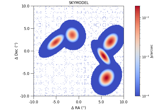
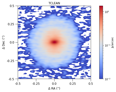
Figure 1: Left: Sky model which serves as an input for creating simulated ALMA Measurement Set. Right: Best tclean image of Sz114 protoplanetary disk from ALMA observations.

2.2 ALMA data

Here we describe archival ALMA observations used to test application of resolve on real-life example. It is important to compare it with a well-understood case, in which the calibration and imaging examples with other tools are already available. We select a protoplanetary disk Sz114 observed within DSHARP ALMA Large Program (Andrews et al., 2018). This was a milestone program for ALMA observatory, showcasing the richness of substructures within disks, often associated with ongoing planet formation. It is therefore especially interesting to search for innovative methods of imaging those data in order to verify current conclusions, as well as open avenue for new studies.

The Sz114 disk shows relatively smooth structure compared with other extreme cases and therefore it serves well as a test case to try to identify underlying structure with resolve. Fig. 1 (right) presents image of the disk obtained with tclean as delivered by the Large Program team (Andrews et al., 2018).

2.3 Imaging of the simulated dataset

First, in order to image the simulated measurement set, we use tclean task in CASA software which implements CLEAN algorithm as in Hogbom 1974 Högbom (1974). We ran tclean without any constraint on where to look for point sources in the image (i.e. without any masking), for 20000 iterations, or until threshold of 0.3 mJy/beam was reached. Pixel size of the reconstructed image is set to 0.1" and image size is set to 512$\times$512 pixels.

This threshold is set based on the earlier, quick tclean, so that the algorithm does not attempt to find sources from the residual image consisting purely of noise. In the default settings, weighting of baselines is set to ’natural’, which means it associate the baseline with weight proportional to the sampling density (i.e. the most covered baselines have the highest weight). Since there is much more baselines sampling the larger scales, this results in putting more weight to lower resolution, which results in achieving lower resolution than the sky model image. Therefore we also attempt an imaging with Briggs weighting with robust parameter 0.5, which moves the balance of weighting toward longer baselines increasing the resolution but decreasing signal-to-noise ratio. The result of the tclean run is presented in Fig. 2 (bottom).

For resolve image of the simulated data we run 30 iterations, using Newton optimizer. We did not make any assumptions on the presence of the point sources in the data. Parameters of the resolve run are summarized in Table 1. For detailed explanation of the parameters see Arras et al. Arras, Philipp et al. (2021).

Table 1: Parameters of the resolve run on simulated dataset (left) and Sz114 ALMA data (right)

Parameter	Mean
Offset	26
Zero mode	1$\pm 0.1$
Fluctuations	5$\pm 1$
Power spectrum slope	-2$\pm 0.5$
Flexibility	1.2$\pm 0.4$
Asperity	0.2$\pm$0.2

Parameter	Mean
Offset	20
Zero mode	1$\pm 0.2$
Fluctuations	3$\pm 1$
Power spectrum slope	-4$\pm 2$
Flexibility	4$\pm 0.8$
Asperity	2$\pm$0.8

2.4 Imaging of the real ALMA observations

For the Sz114 protoplanetary disk observed within DSHAPR ALMA Large Program Andrews et al. (2018) we have created an image from a single spectral window, in order for a direct comparison with resolve, which currently does not have a capability to make images of multiple spectral windows. From the publicly available MS file we extracted spectral window 9 with split task in CASA and binned it into a single channel.

For this tclean run we implemented both standard and multiscale imaging in order to compare the outcomes, since the observed disk presents large variety of spatial scales. We create images with 0.005" and 1024$\times$1024 pixels and run 20000 iterations up to noise threshold of 0.05 mJy is reached. In case of multiscale clean we specified three scales: at 0, 7, and 28 pixels, which means the tclean algorithm iterate in order to find three types of sources in the data: either a point source, which corresponds to scale 0, and extended components with Gaussian shape of 7 and 28 pixels of FWHM. Results of the imaging are presented in Fig. 3 (bottom).

A resolve imaging followed the same procedure as in the simulated data, however, since the weights were obtained with from real observation, this results in more realistic treatment of the uncertainties. Parameters of this run are shown in Tab. 1.

3 Comparison to tclean and resolve

In this initial study of performance of the resolve algorithm in operating with ALMA data, we focus on key aspects of the imaging process: flux recovery – how much flux observed on the sky is recovered by the imaging process and how accurate it is; image quality – effective resolution and dynamic range.

3.1 Simulations

We compare the quality of resolve and tclean imaging of the simple simulated ALMA observation, as described in Section 2.1. Fig. 3 presents resolve image and associated uncertainty map, and tclean image with two different weighting schemes: natural and Briggs weighting with robust parameter of 0.5.

We note that for tclean the imaging resulted with large areas with a negative flux, which do not occur in resolve - positive-only emission is one of the assumptions in the prior. On the uncertainty map produce by resolve we observe much higher confidence associated with the source positions, compared with positions where no significant emission was detected.

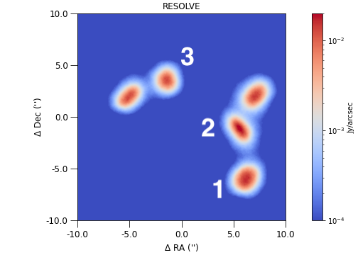
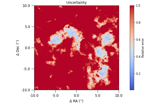
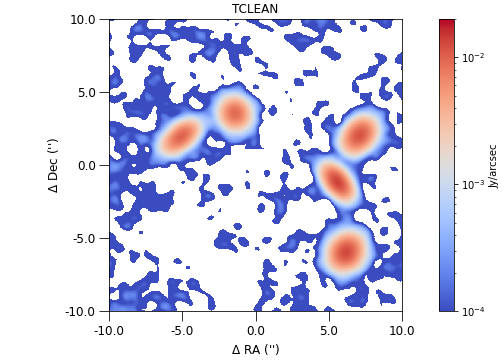
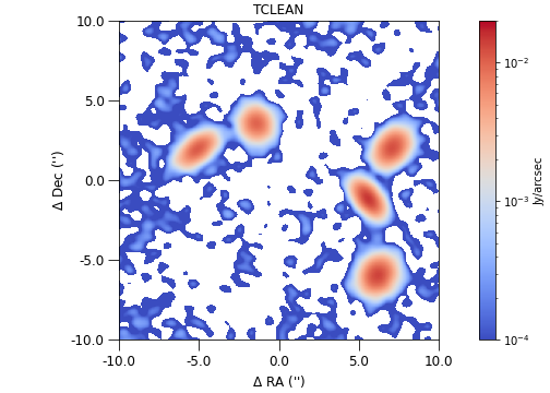
Figure 2: Comparison of the imaging of simulated ALMA observations with resolve and tclean. Top: resolve image (left) with associated uncertainty map. Bottom: two tclean images, left: with natural weighting; right: with Briggs weighting and robust = 0.5.

We measure integrated fluxes of each of the Gaussian components in both imaging methods as well as in the input sky model. Result is presented in Table 1. We can note that resolve and tclean both underestimate the flux of the brightest source (i.e. the Gaussian associated with the largest integrated flux). In case of tclean this can be attributed to imperfect recovery of the signal from the point-spread function, but it is unclear why resolve underpredicts the flux. More extensive runs are needed to investigate this issue.

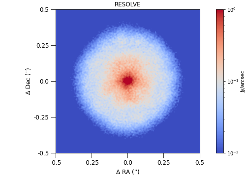
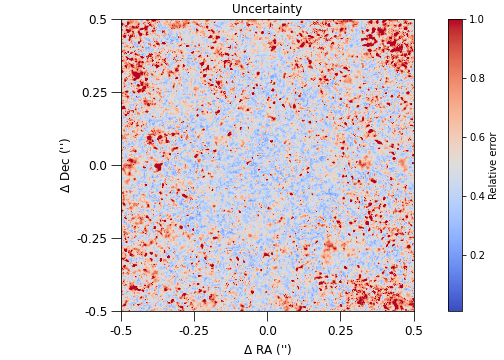
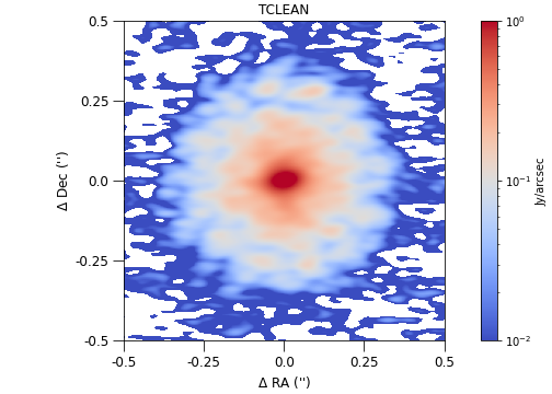
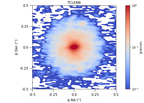
Figure 3: Comparison of the imaging of Sz114 ALMA observations with resolve and tclean. Top: resolve image (left) with associated relative error map. Bottom: two tclean images, left: with standard cleaning algorithm, right: with multi-scale algorithm

On the other hand resolve resolve reaches good accuracy on the other two measured components. We are able to provide much more reliable error bars on resolve by taking the standard deviation of the measured value from all the samples in the final iteration.

Table 2: Peak flux (in Jy arcsec^-2) of different components on the simulated image.

Comp	model	tclean	tclean	resolve
		natural	Briggs
1	34.11	24.67	24.96	26.68$\pm$5.76
2	23.31	21.68	22.19	23.59$\pm$6.72
3	16.69	16.31	16.57	17.82$\pm$3.86

Table 3: Peak (in Jy arcsec^-2) and integrated flux at given radii of the Sz114 disk.

Radius	best	tclean	tclean	resolve
		hogbom	multiscale
peak	1.57	1.55	1.49	5.8$\pm$3.82
0.06	8.63	8.85	8.95	9.48$\pm$1.07
0.15	22.79	22.82	22.53	23.21$\pm$0.68
0.35	47.45	47.07	47.24	47.24$\pm$2.79

3.2 ALMA data

In the case of real ALMA data it is more difficult to assess total recovered flux since we do not have information on true flux. We compare the peak and total flux integrating over different areas of the disk 1. First of all, it can be noted that all tclean images have comparable fluxes, therefore the multiscale did not affect significantly the flux measurements.

In comparison between resolve and tclean, we can see that peak flux measured from resolve image is 3 times as high as the peak in tclean images. This can be purely gridding effect as the pixel scale of the resolve image is much smaller.

At the same time we note slightly comparable values of the integrated flux measured at from different radii of the disk.

At first sight it appears that resolve is able to create super-resolution image of the disk. We can use the uncertainty map to understand what confidence can be associated with those structures. We note on the uncertainty map that we typically achieve better than 20$\%$ confidence on the results but the map also reaches very low confidence in some areas of the map.

4 Conclusions

In this work we apply Bayesian inference and field theory in the framework of Information Field Theory (IFT) using the resolve algorithm, to create images from radio intereferometric observations obtained with ALMA array. The key conclusions are:

• the imaging of simulated ALMA Measurement Set with resolve results in a successful recovery of the flux of the different components in the simulated dataset.

• In one of the first attempts to apply resolve on real ALMA data we obtain a high-fidelity image of protoplanetary disk Sz 114, highlighting the potential of resolve to create super-resolution images.

• For both test cases we obtain a robust estimation of the uncertainties on the measured fluxes, which is one of the major advantages of resolve compared with tclean.

With those encouraging results we highlight further areas where exciting developments can be made: resolve can be used to create spectral cubes, using correlation between channels as additional prior information; create combined maps of different antenna configuration, a particularly challenging case for tclean algorithm and where accurate assessment of the confidence in obtained data is especially necessary.

Acknowledgments: This work made use of the following software: resolve Junklewitz et al. (2015), matplotlib Hunter (2007), NIFTy v.8 Martin Reinecke, Theo Steininger, Marco Selig , astropy Astropy Collaboration (2018), CASA McMullin et al. (2007), This research has made use of NASA’s Astrophysics Data System Bibliographic Services. This paper makes use of the following ALMA data: ADS/JAO.ALMA#2016.1.00484.L. ALMA is a partnership of ESO (representing its member states), NSF (USA) and NINS (Japan), together with NRC (Canada), MOST and ASIAA (Taiwan), and KASI (Republic of Korea), in cooperation with the Republic of Chile. The Joint ALMA Observatory is operated by ESO, AUI/NRAO and NAOJ.

References

References

- Högbom (1974) Högbom, J.A. Aperture Synthesis with a Non-Regular Distribution of Interferometer Baselines. A&AS 1974, 15, 417.
- Junklewitz et al. (2015) Junklewitz, H.; Bell, M.R.; Enßlin, T. A new approach to multifrequency synthesis in radio interferometry. A&A 2015, 581, A59, [arXiv:astro-ph.IM/1401.4711]. doi:\changeurlcolorblack10.1051/0004-6361/201423465.
- Enßlin (2013) Enßlin, T. Information field theory. AIP Conference Proceedings. AIP, 2013. doi:\changeurlcolorblack10.1063/1.4819999.
- Arras, Philipp et al. (2021) Arras, Philipp.; Bester, Hertzog L..; Perley, Richard A..; Leike, Reimar.; Smirnov, Oleg.; Westermann, Rüdiger.; Enßlin, Torsten A.. Comparison of classical and Bayesian imaging in radio interferometry - Cygnus A with CLEAN and resolve. A&A 2021, 646, A84.
- Andrews et al. (2016) Andrews, S.M.; Wilner, D.J.; Zhu, Z.; Birnstiel, T.; Carpenter, J.M.; Pérez, L.M.; Bai, X.N.; Öberg, K.I.; Hughes, A.M.; Isella, A.; Ricci, L. Ringed Substructure and a Gap at 1 au in the Nearest Protoplanetary Disk. ApJ 2016, 820, L40, [arXiv:astro-ph.EP/1603.09352]. doi:\changeurlcolorblack10.3847/2041-8205/820/2/L40.
- Jackson (2008) Jackson, N. Principles of Interferometry. 472; Bacciotti, F.; Testi, L.; Whelan, E., Eds., 2008, Vol. 742, Lecture Notes in Physics, Berlin Springer Verlag, p. 193.
- Thompson et al. (2001) Thompson, A.R.; Moran, J.M.; Swenson, George W., J. Interferometry and Synthesis in Radio Astronomy, 2nd Edition; 2001.
- Cornwell (2008) Cornwell, T.J. Multiscale CLEAN Deconvolution of Radio Synthesis Images. IEEE Journal of Selected Topics in Signal Processing 2008, 2, 793–801. doi:\changeurlcolorblack10.1109/JSTSP.2008.2006388.
- Arras et al. (2018) Arras, P.; Knollmüller, J.; Junklewitz, H.; Enßlin, T.A. Radio Imaging With Information Field Theory. arXiv e-prints 2018, p. arXiv:1803.02174, [arXiv:astro-ph.IM/1803.02174].
- Enßlin et al. (2009) Enßlin, T.A.; Frommert, M.; Kitaura, F.S. Information field theory for cosmological perturbation reconstruction and nonlinear signal analysis 2009. 80, 105005, [arXiv:astro-ph/0806.3474]. doi:\changeurlcolorblack10.1103/PhysRevD.80.105005.
- Selig et al. (2013) Selig, M.; Bell, M.R.; Junklewitz, H.; Oppermann, N.; Reinecke, M.; Greiner, M.; Pachajoa, C.; Enßlin, T.A. NIFTY - Numerical Information Field Theory. A versatile PYTHON library for signal inference. A&A 2013, 554, A26, [arXiv:astro-ph.IM/1301.4499]. doi:\changeurlcolorblack10.1051/0004-6361/201321236.
- Arras et al. (2019) Arras, P.; Baltac, M.; Ensslin, T.A.; Frank, P.; Hutschenreuter, S.; Knollmueller, J.; Leike, R.; Newrzella, M.N.; Platz, L.; Reinecke, M.; Stadler, J. NIFTy5: Numerical Information Field Theory v5. Astrophysics Source Code Library, record ascl:1903.008, 2019, [1903.008].
- Arras et al. (2022) Arras, P.; Frank, P.; Haim, P.; Knollmüller, J.; Leike, R.; Reinecke, M.; Enßlin, T. Variable structures in M87* from space, time and frequency resolved interferometry. Nature Astronomy 2022, 6, 259–269, [arXiv:astro-ph.IM/2002.05218]. doi:\changeurlcolorblack10.1038/s41550-021-01548-0.
- McMullin et al. (2007) McMullin, J.P.; Waters, B.; Schiebel, D.; Young, W.; Golap, K. CASA Architecture and Applications. Astronomical Data Analysis Software and Systems XVI; Shaw, R.A.; Hill, F.; Bell, D.J., Eds., 2007, Vol. 376, ASPC, p. 127.
- Andrews et al. (2018) Andrews, S.M.; Huang, J.; Pérez, L.M.; Isella, A.; Dullemond, C.P.; Kurtovic, N.T.; Guzmán, V.V.; Carpenter, J.M.; Wilner, D.J.; Zhang, S.; Zhu, Z.; Birnstiel, T.; Bai, X.N.; Benisty, M.; Hughes, A.M.; Öberg, K.I.; Ricci, L. The Disk Substructures at High Angular Resolution Project (DSHARP). I. Motivation, Sample, Calibration, and Overview. ApJ 2018, 869, L41, [arXiv:astro-ph.SR/1812.04040]. doi:\changeurlcolorblack10.3847/2041-8213/aaf741.
- Hunter (2007) Hunter, J.D. Matplotlib: A 2D graphics environment. Computer Science and Engineering 2007, 9, 90–95. doi:\changeurlcolorblack10.1109/MCSE.2007.55.
- (17) Martin Reinecke, Theo Steininger, Marco Selig. NIFTy – Numerical Information Field TheorY.
- Astropy Collaboration (2018) Astropy Collaboration. The Astropy Project: Building an Open-science Project and Status of the v2.0 Core Package. AJ 2018, 156, 123, [arXiv:astro-ph.IM/1801.02634]. doi:\changeurlcolorblack10.3847/1538-3881/aabc4f.