Quantum Computation for Periodic Solids in Second Quantization

Abstract

In this work, we present a quantum algorithm for ground-state energy calculations of periodic solids on error-corrected quantum computers. The algorithm is based on the sparse qubitization approach in second quantization and developed for Bloch and Wannier basis sets. We show that Wannier functions require less computational resources with respect to Bloch functions because: (i) the L₁ norm of the Hamiltonian is considerably lower and (ii) the translational symmetry of Wannier functions can be exploited in order to reduce the amount of classical data that must be loaded into the quantum computer. The resource requirements of the quantum algorithm are estimated for periodic solids such as NiO and PdO. These transition metal oxides are industrially relevant for their catalytic properties. We find that ground-state energy estimation of Hamiltonians approximated using 200–900 spin orbitals requires ca. $10{}^{10}$–$10^{12}$ T gates and up to $3\cdot 10^{8}$ physical qubits for a physical error rate of $0.1\%$.

I Introduction

Quantum mechanical simulation of molecules and materials is a promising application area of quantum computers [liu_prospects_2022, bauer_quantum_2020, mcardle_quantum_2020] that will enable the calculation of key properties of chemical systems with controllable errors using physically accurate models. Following Feynman’s original idea of modelling quantum systems on quantum computers [feynman_simulating_1982] and the first formalized procedures for carrying out such simulations [abrams_simulation_1997, abrams_quantum_1999, ortiz_quantum_2001], a plethora of quantum algorithms for calculating energies of molecular systems have been developed in recent years  [aspuru_guzik_simulated_2005, kassal_polynomial_time_2008, whitfield_simulation_2011, seeley_bravyi_kitaev_2012, Toloui_2013, peruzzo_variational_2014, wecker_gate_count_2014, poulin_trotter_2014, hastings_improving_2014, mcclean_exploiting_2014, mcclean_exploiting_2014, babbush_chemical_2015, wecker_progress_2015, babbush_exponentially_2016, mcclean_theory_2016, kivlichan_bounding_2017, babbush_exponentially_2018, babbush_low_depth_2018, poulin_quantum_2018, berry_improved_2018, babbush_encoding_2018, berry_qubitization_2019, higgott2019variational, wang2019accelerated, lee_even_2021, von_burg_quantum_2021, huggins_unbiasing_2022, Su2021]. Similarly, but to a lesser degree, quantum algorithms taking into account the specifics of condensed matter applications have also been conceived. These include the development of different flavors of variational quantum eigensolvers (VQE) [manrique2020momentum, clinton_towards_2022, song_periodic_2022, Yoshioka2022], the quantum imaginary time evolution algorithm [motta_determining_2020], and fault-tolerant algorithms [babbush_low_depth_2018, kivlichan_improved_2020, campbell_early_2021, kanno_resource_2022, flannigan2022propagation, Su2021] for simulation of model Hamiltonians, such as the Hubbard model, as well as first-principles Hamiltonians.

Quantum computers can provide a computational advantage over classical computers only for hard classical problems. These include the simulation of so-called strongly correlated systems and, more practically, problems that are not solved with sufficient accuracy using classical methods with low computation cost — such as Kohn-Sham density functional theory (KS-DFT)) [Hohenberg1964, Kohn1965, Kohn1999] or coupled-cluster theory [vcivzek1966correlation, shavitt2009many]. Notwithstanding varying definitions and interpretations of “strong correlation”, and an ongoing debate regarding the extent to which KS-DFT can describe such systems [cremer2001density, Perdew2021], the general consensus is that molecular and solid state systems with a large number of localised $d$ or $f$ electrons present a significant challenge for classical simulations. Examples of such systems include transition metal oxides such as NiO and PdO used in heterogeneous catalysis applications. The number of localised sites in such systems is formally infinite as the solids should be simulated at the thermodynamic limit. In practice, one restricts calculations to a periodic finite-sized cell (also referred to as supercell) with ca. 30–100 unique transition metal atoms; all other atoms in the solid are replicas of those in this computational cell.

The ability to accurately model the electronic structure of materials such as NiO and PdO would no doubt prove extremely useful in the study of heterogeneous catalysis, a field with no shortage of materials that are poorly described by DFT. It is often the case that the interpretation of calculated results (e.g. regarding trends in activity) must be presented with significant caveats regarding the underlying nature of the models used.

In this work, we focus on the calculation of the ground state energy of electrons in materials within the Born-Oppenheimer approximation [born_zur_1927]. This corresponds to finding the lowest eigenvalue of the electronic Hamiltonian for a fixed position of the nuclei. Two main families of quantum algorithms can perform such calculation: VQE [peruzzo_variational_2014] and quantum phase estimation (QPE) [Kitaev1995, cleve1998quantum, NielsenChuang]. While VQE might have its merits in certain use cases, it appears the emerging consensus is that QPE has a superior scaling with the system size [blunt2022perspective, liu_prospects_2022]. In order to estimate the eigenvalues of the Hamiltonian with QPE, one has to implement a unitary operator encoding the spectrum of the Hamiltonian. QPE requires deep quantum circuits, and as such it will need to run on error-corrected quantum computers. In such error-corrected implementations one must strive to minimize the number of T gates needed to encode the Hamiltonian, as these gates are the costliest to implement (see e.g. [fowler_low_2018]). To this date, the most cost-efficient approaches for such encodings are based on the so-called qubitization technique [low_hamiltonian_2019, poulin_quantum_2018, berry_improved_2018, berry_improved_2018, babbush_encoding_2018, berry_qubitization_2019, von_burg_quantum_2021, lee_even_2021]. Previous work on second quantized Hamiltonians for realistic solid state systems has mainly focused on the Trotterization approach [babbush_low_depth_2018, kivlichan_improved_2020]. In this work, we adapt the sparse qubitization approach to the simulation of crystalline solids with QPE and estimate the resources required for calculating the ground state energy of crystals in error-corrected quantum computers.

The quantum resources required to simulate a Hamiltonian strongly depend on the single-electron basis sets used to represent electron interactions. For crystalline solids, plane waves (PW) currently appear to be one of the most efficient basis sets both in first and second quantization [Su2021, babbush_low_depth_2018]. An advantage of using PW basis sets is the sparse representation of the electronic Hamiltonian. This advantage is always exploited in classical computations such as KS-DFT [Payne1992, Kresse1996prb]. The number of two-body terms in PW representation scales cubically with the size of the basis set. The main disadvantage of such basis sets, however, is that they require a large number of basis functions, especially in all-electron calculations. For crystalline solids one can exploit Bloch functions instead, which are plane waves times a periodic function with the periodicity of the unit cell. In the Bloch representation, the number of terms also scales cubically with the system size, and at the same time such a representation allows using localised atomic orbitals as the periodic constituent of the orbitals. The other commonly used representation in computational condensed matter physics is the Wannier representation, in which orbitals are localized in space [Marzari1997, Skylaris2002, Marzari2012]. Wannier orbitals can be related to Bloch functions through Fourier transformation, and can be localized using unitary optimization in order to produce maximally localized Wannier functions [Marzari1997]. When the periodic function in the Bloch representation is a constant, the Wannier representation coincides with the PW dual representation introduced in the context of quantum computing in Ref. [babbush_low_depth_2018]. At the same time, Wannier orbitals can be spanned in the localised atomic orbital basis which in turn can significantly reduce the size of the basis set for an accurate description of finite band-gap solids. In this work, we investigate Bloch and Wannier representations in the context of qubitized QPE. We note that such basis sets have recently been investigated in the context of the VQE algorithm [clinton_towards_2022].

Quantum computation with qubitization-based QPE requires a large number of gates in a circuit. In order to perform large quantum computations, one has to encode a logical qubit using several physical qubits with a technique known as quantum error correction [shor_scheme_1995, roffe_quantum_2019]. In order to estimate the total number of physical and logical qubits required for the implementation of quantum algorithms as well as their runtime, we have followed Litinski’s approach [litinski_game_2019]. This scheme operates the surface code [fowler_surface_2012] with lattice surgery [horsman_surface_2012, fowler_low_2018], and compiles logical quantum circuits down to just multi-qubit T gates and multi-qubit measurements—all Clifford gates are commuted past the end of the circuit. In this way, runtime is directly related to T-gate count.

The article is organized as follows. In Sec. II, we first describe the relevance of modelling bulk materials such as NiO and PdO for applications to heterogeneous catalysis—an area where quantum computation can provide high accuracy results when error-corrected quantum computers become available. In Sec. III, the Hamiltonian, basis sets, and quantum algorithms for modelling of crystalline solids are introduced. In Sec. LABEL:sec:results, we discuss the performance of quantum algorithms and provide quantum resource estimations for several solid state systems. Finally, discussion and conclusions are presented in Sec. LABEL:sec:disc_and_concl. Detailed logical qubit and Toffoli gate counts of the sparse qubitization are provided in Appendix LABEL:sec:detailed_costings.

II Materials and Heterogeneous Catalysts

Catalysts are used in practically every industrial chemical process, with applications in agriculture, transportation and energy production, among many others. The function of a catalyst to ultimately reduce the energy requirements of a process to make it viable or more efficient means that catalytic processes are a key component for ensuring a sustainable future and reducing human impact on the environment. Transition metal oxide catalysts are essential components for many important industrial processes (such as refining and petrochemistry, fuel cells, hydrogen production, biomass conversion, photocatalysis) where they are used both directly, as the active material (providing the active site), and indirectly, as a support material (commonly as a reducible oxide taking a secondary role in the catalysis). The overall performance of the solid catalyst depends on many factors, including the particle size, particle shape, crystallinity, chemical composition, and all preparation and activation procedures. High catalytic efficiencies are achieved as the number of active surface sites grows, while the structural flexibility of supported metal catalysts (dynamic structural changes) is key for the catalytic reactivity when we consider that the surface sites repeatedly participate in adsorption/desorption cycles.

The systems considered in this work, nickel oxide (NiO) and palladium oxide (PdO), both form the basis of industrially relevant catalyst materials. In the field of energy and environment, natural gas reforming is the most common process used in industry to produce H₂ from fossil fuels, known as methane steam reforming (MSR). Here NiO is reduced to Ni which functions as a high-temperature catalyst. Despite its age and ubiquity, the MSR process still has many technical challenges, for instance around deactivation from carbon whisker formation and stability at high-temperature. Under certain operating conditions, a local oxidizing environment can form within the reactor, leading to the deactivation of Ni due to NiO being present. Thermodynamics can predict the conditions at which this can occur [twigg_catalyst_2018]. However, in general, it is still a challenge to obtain reliable or accurate thermodynamic parameters for strongly correlated oxide materials, especially when they deviate form the bulk limit such as in nanoparticles.

Methane has an estimated greenhouse warming potential (GWP 100) of 27.9 [masson-delmotte_working_2021], meaning its emissions contribute significantly to global warming and climate change; it is therefore necessary to reduce them wherever possible. Among the many different technologies for methane abatement, methane combustion catalysts based on palladium can be found. Such technologies include after-treatment for combustion of natural gas engines (CNG) and diesel oxidation catalysts (DOC) as well as in mine ventilation systems.

In the above applications, methane is efficiently combusted over palladium (or alloyed) oxide catalyst to produce H₂O and CO₂, with activity in this process influenced by a number of factors. A technical target in practical catalysis is to reduce the temperature at which this occurs, allowing for a lower operating temperature and more efficient handling of emissions. Partial oxidation can sometimes occur, and may indeed be desirable in the development of processes to produce precursors for more complex chemicals. The ability to simulate accurately not only the activity but also the selectivity, which is a measure of a catalyst’s ability to promote the formation of the desired product(s) over other possibilities, is crucial to the prediction of new catalysts.

Figure 1(a) shows a schematic of a typical catalyzed reaction. The presence of a catalyst provides additional reaction coordinates, or reaction intermediates, with their own activation energies ($E_{TS1}$, $E_{TS2}$). For an effective catalyst, these energies are necessarily lower than the uncatalyzed activation energy $E_{a}$. In the case of heterogeneous catalysts, reaction intermediates are typically adsorption steps, where one or more of the reactants binds to a surface site of the catalyst. Depending on the complexity of the reaction mechanisms, there may be a large number of these intermediates as well as branches and side reactions that must be considered when studying a reaction in order to determine the key step(s). It is often necessary to find these steps, which govern the activity and/or selectivity of a catalyst, as in doing so, the problem is reduced to fewer dimensions and descriptors that facilitate a more rapid study. For example, in a kinetic analysis the largest activation energy is usually of most interest, as this will be the rate determining step. Whilst this knowledge may be well established in well known reactions, it can be necessary to perform many calculations in more novel applications. Furthermore, whilst the accuracy of current computational approaches may be good enough to predict trends in similar systems, obtaining chemical accuracy and absolute values for detailed kinetic studies remains a challenge. Figure 1(b) shows a typical set of model systems that would be used to estimate the energetics of a heterogeneous catalytic process.

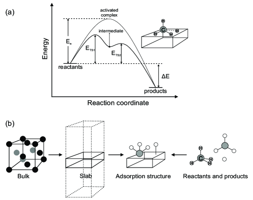
Figure 1: (a) Schematic of a reaction pathway with and without a catalyst, and (b) diagram of the necessary calculation steps required to determine these properties. Relative energies between the reactants, products and intermediates (if they are known) can be calculated via density functional theory or other computational approaches. Reaction barriers for a catalyzed reaction can be approximated via adsorption energy calculations in many cases [cheng_bronstedevanspolanyi_2008], or by transition state searches, which require the calculation of forces as well as the energy.

When running simulations of a catalyst, consideration needs to be made of the question at hand and the level of accuracy that is needed. Broadly speaking, we are interested in activity, selectivity and stability. When simulating activity, we often need a kinetic model which can provide rates or turn-over frequencies. If we are interested in screening for materials, it is often sufficient to correlate these rates with descriptors [toulhoat_kinetic_2003].

For example, following the Sabatier principle [medford_sabatier_2015], which is employed primarily for materials screening, calculating the (heterogeneous) catalytic activity of a material is performed by determining the binding strengths of the reactants, products and any important intermediates of a given reaction with the surface of that material. These binding strengths can be determined from energy calculations using a wide variety of models, each with their own trade-offs between accuracy, transferability and computational cost.

However, if we are interested in predicting reactor performance or process conditions then we need significantly greater precision in the simulated parameters. Likewise, simulating the often subtle differences in competing reactions (which result in different products) typically requires greater accuracy in calculations to predict selectivity.

Whilst the questions of activity and selectivity are crucial for a material’s function as a catalyst, when looking for a technical solution, the question of stability becomes critical. Catalysts often need to operate over many years under harsh conditions (high temperature, pressure, contaminated conditions and, in the case of electrocatalysis, high potentials and corrosive environments). The simulation of stability introduces a whole range of other problems; for instance, predicting morphological changes and thermal degradation of a catalyst requires a large number of calculations, often of large model systems, to allow sintering of nanoparticles or ceramic supports to be conducted. Material complexity (e.g. simulation of realistic metal/ceramic interfaces), bridging time and length scales where accurate atomic-scale materials properties can be fed into multi-scale models, are all open challenges in this area.

DFT is one of the most successful and widely used models for calculating the energies of molecular and solid state systems relevant to industrial processes. It is an ab initio method that uses functionals of the electronic density to calculate energy rather than attempt to deal directly with the many-body wavefunction. In KS-DFT, the electronic density is constructed using a fictitious set of non-interacting single electron wavefunctions and approximating an unknown correction term. This term, known as the exchange-correlation (XC) functional, includes exchange and correlation effects as well as discrepancy between the real and non-interacting kinetic energy. There are many choices, though all of them approximated, for its form.

Ultimately, it is the use of single-particle wavefunctions in DFT that leads to some of its most prominent shortcomings. In the case of NiO, and indeed most transition metal oxides, the strong electron-electron interactions of the d-electrons in these materials is poorly described by approximate KS-DFT, leading to over-delocalisation of these bands (and to the prediction of more metallic electronic structures than the reality). A Hubbard U [kulik_perspective_2015] correction can be used alongside local density approximation (LDA) and generalised gradient approximation (GGA) XC functionals to mitigate this issue in some cases, although it is overly empirical in nature. While the use of hybrid XC functionals such as PBE0 [adamo_toward_1999] can sometimes perform better [mandal_systematic_2019], due to the inclusion of Hartree-Fock exact exchange, the fraction of exact exchange to use can be varied (depending on the XC functional used), which again leads to empirical fitting. Hybrid functionals are also incomplete (and incorrect) in their description of the electronic structure, and are by no means a guaranteed improvement over GGA functionals in their prediction of transition metal oxide properties [coulter_limitations_2013].

To model the bulk properties of materials effectively, the use of periodic boundary conditions (PBCs) is required, allowing for a simulation box to include only the primitive unit cell in highly ordered systems. Even in disordered systems, periodicity is still imposed (on a larger unit cell), as the approximation still provides more representative models than any non-periodic alternative, without extending the system far beyond practical limits.

The study of heterogeneous catalysis primarily concerns the properties of surfaces, so slab models are often used. These are also periodic, albeit in 2 dimensions rather than 3. Bulk calculations are also required in order to determine the surface energies of the facets of a material, which, for example, allow for the prediction of the expected shape of nanoparticles, as well as which facets are most predominant and relevant for catalysis. The stability of a material is another important aspect that can be predicted by energy calculations on bulk systems.

III Methodology

III.1 Hamiltonian for Periodic Systems

The Hamiltonian of interacting electrons in the Born-Oppenheimer approximation can be written as follows:

$$\hat{H}=\hat{H}^{(0)}+\hat{H}^{(1)}+\hat{H}^{(2)},$$ (1)

where $\hat{H}^{(0)}$ is a constant term describing nuclear repulsion, $\hat{H}^{(1)}$ and $\hat{H}^{(2)}$ are one-body and two-body terms, respectively [Stefanucci2013, p. 32]:

$$\hat{H}^{(1)}=\iint\limits d{\bf x}\,d{\bf x}^{\prime}\,\hat{\psi}^{\dagger}({\bf x})h({\bf x},{\bf x}^{\prime})\hat{\psi}({\bf x}^{\prime})$$ (2)

$$\hat{H}^{(2)}=\frac{1}{2}\iint\limits d{\bf x}\,d{\bf x}^{\prime}\,\hat{\psi}^{\dagger}({\bf x})\hat{\psi}^{\dagger}({\bf x}^{\prime})g({\bf x},{\bf x}^{\prime})\hat{\psi}({\bf x}^{\prime})\hat{\psi}({\bf x}),$$ (3)

${\bf x}$ denotes position and spin, $({\bf r},\sigma)$, of an electron and the integration domain is over the volume of the macroscopic crystal, $V$. In this work, we do not consider the external magnetic field or spin-orbit coupling and therefore, the one- and two-body kernels are diagonal w.r.t. spin degrees of freedom. The spatial part of one-body kernel is:

$$h({\bf r})=-\frac{1}{2}\nabla^{2}+U({\bf r})$$ (4)

where $U({\bf r})$ is the nuclei potential

$$U({\bf r})=\sum_{a\in V}\frac{Z_{a}}{|{\bf r}-{\bf P}_{a}|},$$ (5)

$Z_{a}$ and ${\bf P}_{a}$ are the nuclear charge and position of nucleus $a$. The spatial part of two-body kernel is

$$g({\bf r},{\bf r}^{\prime})=g(|{\bf r}-{\bf r}^{\prime}|)=\frac{1}{|{\bf r}-{\bf r}^{\prime}|}$$ (6)

We assume Born-von-Kármán periodic boundary conditions at the boundaries of the macroscopic crystal which is defined by the vectors ${\bf L}_{1},{\bf L}_{2},{\bf L}_{3}$:

$$A({\bf r}+{\bf L}_{\alpha}) =A({\bf r}),\quad A=\hat{\psi},h,U,g\quad\alpha=1,2,3$$ (7)

In this case, the external potential and two-body kernel are defined in terms of their Fourier series:

$$U({\bf r}) =\sum_{a\in V}\sum_{{\bf K}}\frac{4\pi Z_{a}e^{-i{\bf K}{\bf P}_{a}}}{{V\bf K}^{2}}e^{i{\bf K}{\bf r}}$$ (8)

$$g({\bf r}) =\sum_{{\bf K}}\frac{4\pi}{V{\bf K}^{2}}e^{i{\bf K}{\bf r}}$$ (9)

where ${\bf K}$ satisfies:

$${\bf K}{\bf L}_{\alpha}=2\pi m_{\alpha},\quad m_{\alpha}\in\mathbb{Z},\quad\alpha=1,2,3$$ (10)

Crystalline solids consist of unit cells and each unit cell $V_{uc}$ is defined by translation lattice vectors, ${\bf a}_{1},{\bf a}_{2},{\bf a}_{3}$. Each unit cell can be labeled with ${\bf R}$ indicating a node of the Bravais lattice:

$${\bf R}=A^{T}{\bf n};\quad{\bf n}=(n_{1},n_{2},n_{3})^{T},\,n_{\alpha}\in\mathbb{Z};\quad A=[{\bf a}_{1},{\bf a}_{2},{\bf a}_{3}]^{T}$$ (11)

Let $N_{\alpha}\geq 1$ be the number of unit cells along ${\bf a}_{\alpha}$, $n_{\alpha}=0,1,..,N_{\alpha}-1$ and thus, the total number of unit cells which spans the whole finite macroscopic crystal is $N=N_{1}N_{2}N_{3}$. We also introduce the reciprocal lattice which is defined as:

$${\bf G}=B{\bf n};\quad{\bf n}=(n_{1},n_{2},n_{3})^{T},\,n_{\alpha}\in\mathbb{Z};\quad B=[{\bf b}_{1},{\bf b}_{2},{\bf b}_{3}]=2\pi A^{-1}$$ (12)

The vectors ${\bf b}_{1},{\bf b}_{2},{\bf b}_{3}$ and ${\bf a}_{1},{\bf a}_{2},{\bf a}_{3}$ satisfy the following relations:

$${\bf a}_{\alpha}{\bf b}_{\beta}=2\pi\delta_{\alpha\beta}$$ (13)

In the case of crystalline solids, the external potential can also be rewritten in terms of reciprocal lattice vectors, because it is has periodicity of the lattice:

$$U({\bf r}) =\sum_{a\in V_{uc}}\sum_{{\bf G}}\frac{4\pi Z_{a}e^{-i{\bf G}{\bf P}_{a}}}{{V_{uc}\bf G}^{2}}e^{i{\bf G}{\bf r}}$$ (14)

This is similar to Eq. (8) but written for unit-cell periodicity instead of periodicity within macroscopic crystal.

In order to perform practical calculations, one can choose a single-particle basis which is suitable for the problem of interest:

$$\hat{\psi}({\bf x})=\sum_{p,\sigma}\psi_{p}({\bf r})\hat{a}_{p\sigma},$$ (15)

where $p$ can be a set of numbers describing a single particle state such as wave-vector index and band index, for example. The Hamiltonian in the new basis set can be written as:

$$\hat{H}=H^{(0)}+\sum_{pq\sigma}\left(h_{pq}-\frac{1}{2}\sum_{r}g_{prrq}\right)\hat{a}^{\dagger}_{p\sigma}\hat{a}_{q\sigma}+\frac{1}{2}\sum_{pqrs;\sigma,\tau}g_{pqrs}\hat{a}^{\dagger}_{p\sigma}\hat{a}_{q\sigma}\hat{a}^{\dagger}_{r\tau}\hat{a}_{s\tau}$$ (16)

where two-body matrix elements (often referred to as the electron-repulsion integrals or just Coulomb integrals) are:

$$g_{pqrs}=\iint\limits_{V}d^{3}{\bf r}\,d^{3}{\bf r}^{\prime}\,\psi^{*}_{p}({\bf r})\psi_{q}({\bf r})\psi^{*}_{r}({\bf r}^{\prime})\psi_{s}({\bf r}^{\prime})g(|{\bf r}-{\bf r}^{\prime}|)$$ (17)

From this definition, $g_{pqrs}$ obeys the 4-fold symmetry relations:

$$g_{pqrs}=g_{rspq}=g_{qpsr}^{*}=g_{srqp}^{*}$$ (18)

If coefficients are real then $g_{pqrs}$ obeys the 8-fold symmetry relations:

$$g_{pqrs}=g_{pqsr}=g_{qprs}=g_{qpsr}=g_{rspq}=g_{srpq}=g_{rsqp}=g_{srqp}$$ (19)

The set of orbitals $\{\psi_{p}({\bf r})\}$ should be an orthonormal basis set which satisfies the periodic boundary conditions. Below we describe two basis sets which are commonly used in computational condensed matter physics. Further in the text, the number of spatial orbitals per unit cell is denoted as $M$ (the number of bands) while the total number of spatial orbitals in the crystal is $P=MN$.

III.1.1 Bloch Functions as a Basis Set

Bloch functions are the solution of a mean-field problem in a periodic potential. The Bloch functions can be written as follows [KittelISSP, p.167]:

$$\psi_{{\bf k}j}({\bf r})=e^{i{\bf k}{\bf r}}u_{{\bf k}j}({\bf r})$$ (20)

where $u_{{\bf k}}({\bf r})$ is periodic function with periodicity of the unit cell, $u_{{\bf k}}({\bf r})=u_{{\bf k}}({\bf r}+{\bf R})$, $j$ is the band index, $0\leq j\leq M$ and ${\bf k}=(k_{1},k_{2},k_{3})^{T}$ is the wave vector belonging to the first Brillouin zone which can be defined as:

$$k_{\alpha}=\sum_{\beta=1,2,3}B_{\alpha\beta}\frac{g_{\beta}}{N_{\beta}},$$ (21)

where $g_{\beta}$ is an integer such that

$$-\frac{N_{\alpha}}{2}<g_{\alpha}\leq\frac{N_{\alpha}}{2}$$ (22)

The larger the size of the macroscopic crystal, the larger the number of $k$-points in the Brillouin zone as can be seen from (22). Using Bloch functions as the basis set

$$\hat{\psi}({\bf x})=\sum_{{\bf k}j}\psi_{{\bf k}j}({\bf r}){\hat{c}}_{{\bf k}j\sigma}$$ (23)

the Hamiltonian can be written as:

$$\hat{H}=H^{(0)}+\sum_{{\bf k}ij\sigma}\tilde{h}_{{\bf k}ij}{\hat{c}}^{\dagger}_{{\bf k}i\sigma}{\hat{c}}_{{\bf k}j\sigma}+\frac{1}{2N}\sum_{\sigma,\sigma^{\prime}}\sum_{ijlm}\sum_{{\bf k}{\bf q}{\bf k}^{\prime}{\bf q}^{\prime}}\left(\sum_{{\bf G}}\delta_{{\bf q}+{\bf q}^{\prime}-{\bf k}-{\bf k}^{\prime},{\bf G}}\right)\tilde{g}_{{\bf k}i,{\bf q}j,{\bf k}^{\prime}l,{\bf q}^{\prime}m}{\hat{c}}^{\dagger}_{{\bf k}i\sigma}{\hat{c}}^{\dagger}_{{\bf k}^{\prime}l\sigma^{\prime}}{\hat{c}}_{{\bf q}^{\prime}m\sigma^{\prime}}{\hat{c}}_{{\bf q}j\sigma}$$ (24)

where we used the convention that the Bloch functions are normalized in the unit cell. Due to $\sum_{{\bf G}}\delta_{{\bf q}+{\bf q}^{\prime}-{\bf k}-{\bf k}^{\prime},{\bf G}}$, the number of two-body terms scales as $O(N^{3})$, the same as in the plane-wave basis set [babbush_low_depth_2018]. One- and two-body matrix elements are defined as:

$$\tilde{h}_{{\bf k}ij}=\int\limits_{V_{uc}}d^{3}{\bf r}\,\psi^{*}_{{\bf k}i}({\bf r})h({\bf r})\psi_{{\bf k}^{\prime}j}({\bf r})$$ (25)

and

$$\tilde{g}_{{\bf k}i,{\bf q}j,{\bf k}^{\prime}l,{\bf q}^{\prime}m}=\int\limits_{V_{uc}}d^{3}{\bf r}\,\psi_{{\bf k}i}^{*}({\bf r})\psi_{{\bf q}j}({\bf r})\int\limits_{V_{uc}}d^{3}{\bf r}\,^{\prime}\psi_{{\bf k}^{\prime}l}^{*}({\bf r}^{\prime})\psi_{{\bf q}^{\prime}m}({\bf r}^{\prime})g_{{\bf q}^{\prime}-{\bf k}^{\prime}}({\bf r}-{\bf r}^{\prime}),$$ (26)

where

$$g_{{\bf q}-{\bf k}}({\bf r}-{\bf r}^{\prime})=\sum_{{\bf G}}\frac{4\pi}{({\bf q}-{\bf k}+{\bf G})^{2}V_{uc}}e^{i({\bf q}-{\bf k}+{\bf G})({\bf r}-{\bf r}^{\prime})}$$ (27)

and $V_{uc}$ is the volume of the unit cell. Coefficients in the Hamiltonian are usually complex and the two-body terms obey 4-fold symmetry (18). The composite index from Sec. III.1 indicates both band and wave vector, $p=({\bf k},i)$, $q=({\bf q},j)$, $r=({\bf k}^{\prime},l)$, $s=({\bf q}^{\prime},m)$.

III.1.2 Wannier Functions as a Basis Set

Wannier functions are the set of localized orbitals which obey the translational symmetry of the crystal:

$$\phi_{{\bf R}j}({\bf r}-{\bf R}^{\prime})=\phi_{{\bf R}+{\bf R}^{\prime}j}({\bf r})$$ (28)

Such localized orbitals can be obtained by carrying out a localization procedure in the supercell or applying a Fourier transformation to the Bloch orbitals [Marzari2012]:

$$\phi_{{\bf R}j}({\bf r})=\frac{1}{N}\sum_{{\bf k}}e^{-i{\bf k}{\bf R}}\sum_{m}\psi_{{\bf k}m}({\bf r})U_{mj}^{({\bf k})},$$ (29)

where unitary matrices can be chosen according to localization criteria such as, for example, Foster-Boys [Foster1960] (Maximally Localized Wannier orbitals [Marzari1997]) or Pipek-Mezey [Pipek1989, lehtola_pipek_2012, Jonsson2017]. Contrary to Bloch functions, these functions can be chosen to be real valued [Marzari2012]. In the Wannier basis set

$$\hat{\psi}({\bf x})=\sum_{{\bf R}j}\phi_{{\bf R}j}({\bf r}){\hat{a}}_{{\bf R}j\sigma}$$ (30)

the Hamiltonian is

$$\hat{H}=H^{(0)}+\sum_{{\bf R}{\bf R}^{\prime}ij\sigma}h_{{\bf R}p,{\bf R}^{\prime}q}{\hat{a}}^{\dagger}_{{\bf R}i\sigma}{\hat{a}}_{{\bf R}j\sigma}+\frac{1}{2}\sum_{\sigma,\sigma^{\prime}}\sum_{ijlm}\sum_{{\bf R}{\bf T}{\bf R}^{\prime}{\bf T}^{\prime}}g_{{\bf R}i,{\bf T}j,{\bf R}^{\prime}l,{\bf T}^{\prime}m}{\hat{a}}^{\dagger}_{{\bf R}i\sigma}{\hat{a}}^{\dagger}_{{\bf R}^{\prime}l\sigma^{\prime}}{\hat{a}}_{{\bf T}^{\prime}m\sigma^{\prime}}{\hat{a}}_{{\bf T}j\sigma}$$ (31)

with matrix elements:

$$h_{{\bf R}i,{\bf R}^{\prime}j}=\int\limits_{V}d^{3}{\bf r}\,\phi^{*}_{{\bf R}i}({\bf r})h({\bf r})\phi_{{\bf R}^{\prime}j}({\bf r})$$ (32)

and

$$g_{{\bf R}i,{\bf T}j,{\bf R}^{\prime}l,{\bf T}^{\prime}m}=\int\limits_{V}d^{3}{\bf r}\,\phi_{{\bf R}i}^{*}({\bf r})\phi_{{\bf T}j}({\bf r})\int\limits_{V}d^{3}{\bf r}\,^{\prime}\phi_{{\bf R}^{\prime}l}^{*}({\bf r}^{\prime})\phi_{{\bf T}^{\prime}m}({\bf r}^{\prime})g({\bf r}-{\bf r}^{\prime})$$ (33)

which satisfy the following relations:

$$h_{{\bf R}i,{\bf R}^{\prime}j}=h_{0i,{\bf R}^{\prime}-{\bf R}j}$$ (34)

$$v_{{\bf R}i{\bf T}j{\bf R}^{\prime}l{\bf T}^{\prime}m}=v_{0i,{\bf T}-{\bf R}j,{\bf R}^{\prime}-{\bf R}l,{\bf T}^{\prime}-{\bf R}m}$$ (35)

This is due to the fact that Wannier functions obey Eq. (28). In this paper we don’t construct Wannier functions from Bloch orbitals but rather choose natural atomic orbitals in the supercell calculations (see Section LABEL:subsec:_classical_computational_details for computational details). Since the two-body term is real, it satisfies Eq. (19). The composite index from Sec. III.1 indicates both band and unit cell indices, $p=({\bf R},j)$, $q=({\bf T},j)$, $r=({\bf R}^{\prime},l)$, $s=({\bf T}^{\prime},m)$.

III.1.3 Majorana Representation

Majorana operators represent a convenient choice for working with quantum computing algorithms. The reason is that each Majorana operator is Hermitian and can be mapped onto one Pauli string using a qubit representation and, as a result, any unique product of Majorana operators is one Pauli string. The actual qubit representation depends on the choice of transformation such as the Jordan-Wigner [Jordan1928, ortiz_quantum_2001] or Bravyi-Kitaev [Bravyi2002, seeley_bravyi_kitaev_2012]. However, some properties of the Hamiltonian which do not depend on the choice of qubit mapping can conveniently be obtained in Majorana representation. We will use this representation in order to generalize the sparse qubitization approach on Hamiltonians with complex coefficients. Majorana operators are defined as:

$$\hat{\gamma}_{p\sigma,0} =\hat{a}_{p\sigma}+\hat{a}^{\dagger}_{p\sigma}$$ (36)

$$\hat{\gamma}_{p\sigma,1} =-i(\hat{a}_{p\sigma}-\hat{a}^{\dagger}_{p\sigma})$$ (37)

with an additional binary index specifying the Majorana type.

They satisfy the following anti-commutation relations:

$$\{\hat{\gamma}_{p\sigma,k},\hat{\gamma}_{q\tau,j}\}=2\delta_{pq}\delta_{\sigma\tau}\delta_{kj}$$ (38)

Following Refs. [von_burg_quantum_2021, Koridon2021], the constant, one-body and two-body terms of the Hamiltonian (16) in Majorana representation can be written as follows:

$$\tilde{H}_{0}=H_{0}+\sum_{p}h_{pp}+\frac{1}{2}\sum_{pq}\left(g_{ppqq}-\frac{1}{2}g_{pqqp}\right)$$ (39)

$$\hat{\tilde{H}}^{(1)} =\frac{i}{2}\sum_{p\leq q}{\rm Re}\left(h_{pq}+\frac{1}{2}\sum_{r}\left(2g_{pqrr}-g_{prrq}\right)\right)\left(\frac{1}{2}\right)^{\delta_{pq}}\sum_{\sigma;j\neq k}(-1)^{j}\hat{\gamma}_{p\sigma,j}\hat{\gamma}_{q\sigma,k}$$ (40)

$$+\frac{i}{2}\sum_{p<q}{\rm Im}\left(h_{pq}+\frac{1}{2}\sum_{r}\left(2g_{pqrr}-g_{prrq}\right)\right)\sum_{\sigma;j}\hat{\gamma}_{p\sigma,j}\hat{\gamma}_{q\sigma,j}$$ (41)

$$\hat{\tilde{H}}^{(2)} =\frac{1}{4}\sum_{\begin{subarray}{c}p\leq q,r\leq s\\ (p,q)\leq(r,s)\end{subarray}}B_{pqrs}\left(\frac{1}{2}\right)^{\delta_{pq}+\delta_{rs}+\delta_{(p,q),(r,s)}}\sum_{\sigma\neq\tau,j\neq k,l\neq m}\hat{\gamma}_{p\sigma,j}\hat{\gamma}_{q\sigma,k}\hat{\gamma}_{r\tau,l}\hat{\gamma}_{s\tau,m}(-1)^{j+m}$$ (42)

$$+\frac{1}{4}\sum_{\begin{subarray}{c}p<q,r<s\\ (p,q)\leq(r,s)\end{subarray}}F_{pqrs}\left(\frac{1}{2}\right)^{\delta_{(p,q),(r,s)}}\sum_{\sigma\neq\tau;j,k}\hat{\gamma}_{p\sigma,j}\hat{\gamma}_{q\sigma,j}\hat{\gamma}_{r\tau,k}\hat{\gamma}_{s\tau,k}(-1)^{j+k}$$ (43)

$$+\frac{1}{4}\sum_{p\leq q,r<s}(-1)C_{pqrs}\left(\frac{1}{2}\right)^{\delta_{pq}}\sum_{\sigma\neq\tau;j\neq k;l}\hat{\gamma}_{p\sigma,j}\hat{\gamma}_{q\sigma,k}\hat{\gamma}_{r\tau,l}\hat{\gamma}_{s\tau,l}(-1)^{j}$$ (44)

$$+\frac{1}{4}\sum_{\begin{subarray}{c}p<q,r<s\\ (p,q)\leq(r,s)\end{subarray}}\left(F_{pqrs}+B_{prqs}-B_{psqr}\right)\left(\frac{1}{2}\right)^{\delta_{(p,q),(r,s)}}\sum_{\sigma,j\neq k}\hat{\gamma}_{p\sigma,j}\hat{\gamma}_{q\sigma,j}\hat{\gamma}_{r\sigma,k}\hat{\gamma}_{s\sigma,k}$$ (45)

$$+\frac{1}{4}\sum_{p<q<r<s}(F_{pqrs}-F_{prqs}+F_{psqr})\sum_{\sigma,j}\hat{\gamma}_{p\sigma,j}\hat{\gamma}_{q\sigma,j}\hat{\gamma}_{r\sigma,j}\hat{\gamma}_{s\sigma,j}$$ (46)

$$+\frac{1}{4}\sum_{p,q<r<s}\left(C_{pqrs}-C_{prqs}+C_{psqr}\right)\sum_{\sigma,j\neq k}\hat{\gamma}_{p\sigma,j}\hat{\gamma}_{q\sigma,k}\hat{\gamma}_{r\sigma,k}\hat{\gamma}_{s\sigma,k}(-1)^{j}$$ (47)

where the tensors

$$B_{pqrs}=\frac{{\rm Re}(g_{pqrs}+g_{pqsr})}{2}=\frac{g_{pqrs}+g_{qpsr}+g_{pqsr}+g_{qprs}}{4}$$ (48)

$$C_{pqrs}=\frac{{\rm Im}(g_{pqrs}-g_{pqsr})}{2}=\frac{g_{pqrs}-g_{qpsr}-g_{pqsr}+g_{qprs}}{4i}$$ (49)

$$F_{pqrs}=\frac{{\rm Re}(g_{pqrs}-g_{pqsr})}{2}=\frac{g_{pqrs}+g_{qpsr}-g_{pqsr}-g_{qprs}}{4}$$ (50)

$B_{pqrs}$ is symmetric w.r.t. $(p,q)$ and symmetric w.r.t. $(r,s)$, $C_{pqrs}$ is symmetric w.r.t. $(p,q)$ and antisymmetric w.r.t. $(r,s)$, $F_{pqrs}$ is antisymmetric w.r.t. $(p,q)$ and antisymmetric w.r.t. $(r,s)$, $B$ and $F$ are symmetric w.r.t. interchange of pairs $(p,q)$, $(r,s)$, while $C_{pqrs}$ is not.
The reverse relation is

$$g_{pqrs}=B_{pqrs}+F_{pqrs}+i(C_{rspq}+C_{pqrs}).$$ (51)

This representation of the Hamiltonian is valid for both Bloch and Wannier orbitals and the only differences are indices labeling states and the value of coefficients. For real-valued Wannier functions, only the $B_{pqrs}$ tensor is non-zero while for complex-valued orbitals, such as Bloch functions, all tensors need to be taken into account as coefficients of the Hamiltonian in Eq. (16) can be complex. The Hamiltonian in Majorana representation (39)–(47) provides a decomposition in a linear combination of unitaries (LCU [Childs2012]) and the entry-wise L₁ norm of such a Hamiltonian, which is the same in any qubit representation [Koridon2021], can be written as:

$$\alpha=\lambda_{0}+\lambda=\lambda_{0}+\lambda_{1}+\lambda_{2}$$ (52)

where

$$\lambda_{0}=\left|H_{0}+\sum_{p}h_{pp}+\frac{1}{4}\sum_{pr}\left(2g_{pprr}-g_{prrp}\right)\right|$$ (53)

$$\lambda_{1} =\sum_{pq}\left|{\rm Re}\left(h_{pq}+\frac{1}{2}\sum_{r}\left(2g_{pqrr}-g_{prrq}\right)\right)\right|+2\sum_{p<q}\left|{\rm Im}\left(h_{pq}+\frac{1}{2}\sum_{r}\left(2g_{pqrr}-g_{prrq}\right)\right)\right|$$ (54)

$$\lambda_{2} =\frac{1}{4}\sum_{pqrs}\left|B_{pqrs}\right|+\sum_{p<q,r<s}\left|F_{pqrs}\right|+\sum_{p,q,r<s}\left|C_{pqrs}\right|+\frac{1}{2}\sum_{p<q,r<s}\left|F_{pqrs}+B_{prqs}-B_{psqr}\right|+$$ (55)

$$+\sum_{p<q<r<s}\left|F_{pqrs}-F_{prqs}+F_{psqr}\right|+\sum_{p,q<r<s}\left|C_{pqrs}-C_{prqs}+C_{psqr}\right|$$ (56)

In the context of quantum computation, the magnitude of $\lambda=\lambda_{1}+\lambda_{2}$ defines the number of repetitions of controlled-unitary in QPE as discussed below.

III.2 Quantum Algorithms

QPE [Kitaev1995, NielsenChuang] allows to determine the phase of a unitary operator which is implemented in the quantum circuit. Originally, Hamiltonian simulation with the choice of unitary

$$U=e^{iHt}$$ (57)

was used, as the time evolution operator can be implemented with Trotterization [suzuki1991general, childs2018toward] and its phases $E_{j}t$ are directly related to the system’s energies $E_{j}$. Other methods for Hamiltonian simulation have since been developed, including Taylor series [babbush_exponentially_2016, babbush_exponentially_2018, babbush_low_depth_2018] and randomised methods [campbell_random_2019, kivlichan_phase_2019, wan_randomized_2022].

Instead of the time evolution operator (57), one can apply QPE to a unitary walk operator $W$ with eigenvalues $e^{\pm i\arccos(E_{j}/\lambda)}$, from whose phases the Hamiltonian energies can readily be retrieved. This is the approach of more recent qubitisation methods [poulin_quantum_2018, berry_improved_2018]. The normalization factor $\lambda$ is the $L_{1}$ norm of Hamiltonian’s coefficients in an LCU decomposition, and ensures that all energies correspond to phases between $0$ and $2\pi$. The walk operator is constructed from a reflection along with a block encoding of $H/\lambda$. The starting point for a block encoding is an LCU decomposition of the Hamiltonian

$$H=\sum_{i=1}^{d}w_{i}H_{i},\ w_{i}\in\mathbb{R}^{+}$$ (58)

into simpler unitary operators $H_{i}$ that can be readily implemented on a quantum computer. In our case, the LCU decomposition of the Hamiltonian is given in section III.1.3, and the $H_{i}$ consist of strings of up to four Majorana fermions that can be implemented in the Jordan-Wigner representation with a ranged operation [babbush_encoding_2018]. The two operators

$$\operatorname{SELECT}\ket{i}\ket{\psi}=\ket{i}H_{i}\ket{\psi}\ \text{and}\ \operatorname{PREPARE}\ket{0}=\sum_{i=1}^{d}\sqrt{\frac{{w_{i}}}{\lambda}}\ket{i}\ \text{with}\ \lambda=\sum_{i=1}^{d}|w_{i}|$$ (59)

facilitate a block encoding of $H/\lambda$ because

$$\bra{0}(\operatorname{UNPREPARE}\otimes\mathbbm{1})\operatorname{SELECT}(\operatorname{PREPARE}\otimes\mathbbm{1})\ket{0}=H/\lambda$$ (60)

with $\operatorname{UNPREPARE}=\operatorname{PREPARE}^{-1}$.

The leading order cost of qubitization algorithms is typically proportional to $O(\lambda\sqrt{d}/\epsilon)$. A multiplicative $\lambda$ is needed to maintain a fixed energy accuracy $\epsilon$ in phase estimation despite the normalization of the Hamiltonian by $\lambda$. Meanwhile, the $\sqrt{d}$ stems from data loading. The values of the $d$ coefficients of the LCU $\omega_{i}$ can be loaded with Toffoli cost of order $O(\sqrt{d})$ with a select-swap network [Low2018Trading] (also dubbed QROAM [berry_qubitization_2019]) at the expense of $O(\sqrt{d})$ ancilla qubits.

Various implementations of the qubitization walk operator [babbush_encoding_2018, von_burg_quantum_2021, lee_even_2021, berry_qubitization_2019] factorize the Hamiltonian to find alternative LCUs with lower $d$ and/or $\lambda$. They also show bespoke implementations of PREPARE and SELECT matching the choice of LCU. We base our method on the sparse qubitization method [berry_qubitization_2019, lee_even_2021], which does not factorize the Hamiltonian, but instead exploits sparsity. In the next section, we will give an overview of that method. Then we will describe how we have adapted and extended the method to deal with Bloch and Wannier basis sets. We focus on the asymptotically dominant costs and confine detailed Toffoli and qubit number costings to Appendix LABEL:sec:detailed_costings. The number of T gates is 4 times the number of Toffoli gates [Gidney2018Halving, babbush_encoding_2018].

III.2.1 Overview of Sparse Qubitization

In this section we outline the original sparse qubitization algorithm which has been used for simulation of real Hamiltonians which satisfy 8-fold symmetry relations (19). It was first developed in [berry_qubitization_2019] and improved in [lee_even_2021], Appendix A, on which we base our exposition. Our modifications to this algorithm are presented in the Secs. III.2.2 and LABEL:sec:Wannier_sparse_qubitisation. For simplicity of this summary, we focus on the Hamiltonian’s two-body terms, of which there are significantly more than one-body terms. The main insight the sparse qubitization algorithm [berry_qubitization_2019, lee_even_2021] uses is that the Hamiltonian’s LCU decomposition into unitaries $Q$

$$H=\frac{1}{8}\sum_{pqrs,\sigma,\tau}V_{pqrs}Q_{pq\sigma}Q_{rs\tau}$$ (61)

is very sparse with respect to the orbital indices, $(p,q,r,s)$, and spin indices, $(\sigma,\tau)$, especially if small coefficients $V_{pqrs}$ are approximated to zero. Thus one can save on quantum resources required for the data loading: Instead of loading the coefficients for all values of $p,q,r,s,\sigma,\tau$, only a unique set of non-zero coefficients is loaded onto the quantum computer and the rest of the Hamiltonian can be restored using symmetry restoration circuits. Let these non-zero coefficients be indexed by $l=1\ldots d$ in an arbitrary way, such that we must load only $d$ data items. While the scaling of $d$ with the total number of spatial orbitals, $P$, is still expected to be the same as the full number of electron repulsion integrals,

$$d\sim O(P^{4}),$$ (62)

one can truncate small coefficients and reduce $d$. Each data item to be loaded consists of the value of the coefficient $V_{pqrs}$ as well as the corresponding indices $p,q,r,s,\sigma,\tau$ that allow to apply the correct unitary $Q_{pq\sigma}Q_{rs\tau}$. QROAM allows to load these as qubit bitstrings. However, PREPARE requires the coefficient values as amplitudes of the state, not bitstrings. This gap is bridged by instead loading so-called “keep-probabilities” and performing coherent alias sampling [babbush_encoding_2018]. Fig. 2 shows a sketch of the PREPARE operator.

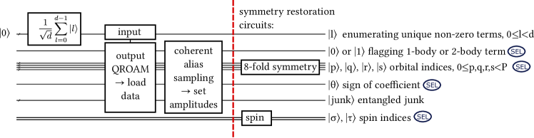
Figure 2: PREPARE operator for the original sparse qubitization method [berry_qubitization_2019, lee_even_2021], outlined in Sec. III.2.1. It prepares a superposition of product states describing the Hamiltonian’s LCU: The amplitudes in the superposition are the (square root modulus of the) LCU’s coefficients $\propto V_{pqrs}$, whilst the corresponding product state specifies the unitary operator $Q_{pq\sigma}Q_{rs\tau}$. The state is entangled to an additional junk register, such as the additional qubits needed for coherent alias sampling. Only the qubits indicated with  are used as controls by the SELECT operator. At the vertical dashed line (red), the prepared state describes just one symmetry sector w.r.t. spin symmetry and 8-fold symmetry. This reduces the amount of data to be loaded, which is the most expensive step in the circuit. The superposition is then enlarged to more product states covering all symmetry sectors with the symmetry restoration circuits. Note that ancilla qubits (such as in the QROAM or 8-fold symmetry restoration circuit) are not depicted. Despite becoming entangled with the other qubits, like $\ket{\text{junk}}$, they do not affect the rest of the circuit.

The number of data items $d$ to load can be reduced further by leveraging symmetries of the Hamiltonian that cause multiple identical coefficients. First of all, coefficient values are independent of spin. Thus we must only load one coefficient, and the other identical terms can be restored in the quantum circuit. Likewise, for a given permutation of orbital indices, eight coefficients which posses 8-fold symmetries (see Eqs (19)) can also be restored in the quantum circuit using only one set of orbital indices. This reduces the number of terms to be loaded $d$ by approximately a factor of 8.

The PREPARE operator is implemented in the following steps illustrated in Fig. 2 (see [berry_qubitization_2019, lee_even_2021] for details):

Equal superposition state

Prepare $\frac{1}{\sqrt{d}}\sum_{l=0}^{d-1}\ket{l}$ , where $d$ is the number of non-zero LCU terms (up to 8-fold and spin symmetries). This uses ancillas for amplitude amplification not shown in the figure.

Data loading

A QROAM loads data of width $m$ qubits. In principle, these $m$ qubits include the value of the coefficient indices $p(l),q(l),r(l),s(l)$ along with the value $w_{l}=|V_{p(l)q(l)r(l)s(l)}|/8$ and its sign $\theta$.

However, in practice, in order to perform coherent alias sampling, slightly different data items must be loaded [babbush_encoding_2018]. Instead of the coefficient value $V_{pqrs}$, a data field of $\aleph$ qubits (so-called “keep-probability”) is needed. $\aleph$ determines the accuracy with which the coefficients $V_{pqrs}$ are ultimately loaded and can be computed with (LABEL:eq:aleph). Further, coherent alias sampling requires two values of the other data to be loaded (indices $p,q,r,s$ and $\theta$ and a qubit not mentioned here to distinguish between one- and two-body terms) [babbush_encoding_2018]. Thus,

$$m=\aleph+2(4\lceil\log P\rceil+2)$$ (63)

where $P$ is the number of spatial orbitals ($2P$ is the number of spin orbitals).

The QROAM is the asymptotically most expensive step with Toffoli cost

$$\lceil d/\kappa\rceil+m(\kappa-1).$$ (64)

Adjusting $\kappa$ (which must be a power of 2) leads to a tradeoff between Toffoli cost and ancilla qubit count [Low2018Trading]

$$m\kappa+\lceil\log(d/\kappa)\rceil.$$ (65)

Choosing $\kappa\sim\sqrt{d}$ to optimise Toffoli cost, both Toffoli and ancilla count of the data lookup asymptotically follow (dropping logarithmic factors)

$$\sim O(\sqrt{d})\sim O(P^{2}).$$ (66)

While the QROAM lookup will also have to be uncomputed in UNPREPARE, the cost is lower because it doesn’t depend on the size $m$ of the data items when using a measurement-based uncomputation scheme [berry_qubitization_2019].

Coherent alias sampling

From the information thus loaded, coherent alias sampling then creates the state

$$\sum_{l=0}^{d-1}\sqrt{\frac{w_{i}}{\lambda}}\ket{l}\ket{0/1}\ket{p}\ket{q}\ket{r}\ket{s}\ket{\theta}\ket{\textrm{junk}_{l}},$$ (67)

which is entangled to some $\ket{\textrm{junk}_{l}}$ that is not relevant. The second register, 0 or 1, flags one- or two-body terms, respectively.

Symmetry restoration

Now, the spin symmetry and 8-fold symmetry must be restored. Two new qubits encoding spin $\ket{\sigma}$ and $\ket{\tau}$ in the state $(\ket{0}+\ket{1})/\sqrt{2}$ are added as further tensor product factors. When the tensor product is expanded, it quadruples the number of states in the superposition (67).

To restore 8-fold symmetry, similarly three qubits $(\ket{0}+\ket{1})/\sqrt{2}$ for each of the symmetries $p\leftrightarrow q,r\leftrightarrow s,(p,q)\leftrightarrow(r,s)$ are added as tensor product factors. Swaps controlled on these qubits then swap $p,q,r,s$ registers depending on the symmetry.

The result is a state describing the full LCU in (61). A subtlety of symmetry restorations is that slightly different values of $w_{i}$ must be loaded by the QROAM, because the symmetry restoration accumulates factors of $1/\sqrt{2}$. Yet this does not affect the overall subnormalisation $\lambda$ of the Hamiltonian.

Next, a SELECT operator selects the correct unitary for the $p,q,r,s,\sigma$ and $\tau$ indices. The UNPREPARE operator uncomputes PREPARE. Using measurement based uncomputation, this is much more efficient than PREPARE [berry_qubitization_2019]. The total leading order Toffoli cost is

$$\left\lceil\frac{\pi\lambda}{2\epsilon_{\rm QPE}}\right\rceil\cdot\left(\left\lceil\frac{d}{\kappa}\right\rceil+m(\kappa-1)\right),$$ (68)

the product of the QROAM cost for data loading (64) with the number of iterations of the walk operator $\lceil\pi\lambda/(2\epsilon_{\rm QPE})\rceil$. The normalisation factor, $\lambda$, together with the desired accuracy, $\epsilon_{\rm QPE}$, determine the number of iterations of the walk operator required for phase estimation.

III.2.2 Generalization of Sparse Qubitization for Bloch Basis Functions

While the original sparse qubitization method supports Hamiltonians with real electron repulsion integrals only, Bloch orbitals usually lead to complex coefficients. We generalise the sparse method to complex Hamiltonians by expanding the Hamiltonian in Majorana strings III.1.3 and instead of working with 8-fold symmetry restoration circuits, we introduce Majorana type restoration circuits. For a real Hamiltonian the expansion (40)–(47) only contains the terms (40), (42), and (45). The other terms arise for complex Hamiltonians. The coefficients of the Majorana strings are all real (or purely imaginary for the one-body terms) due to the Hamiltonian’s Hermeticity.

We use a SELECT operator [babbush_encoding_2018, von_burg_quantum_2021] that allows to select Majorana strings based on: the indices $p,q,r,s$; spin indices $\sigma,\tau$; and four Majorana type indices $j_{1}$ through $j_{4}$—as they appear in the Hamiltonian (section III.1.3). In addition, the correct sign of the LCU coefficient is selected based on a $\ket{\theta}$ qubit. In Fig. 3, the control qubits for SELECT are indicated by . The indices $p,q,r,s$ index the Bloch basis functions (20), and as such they are composite indices, each consisting of band index and $k$-wave-vector index. For the Bloch basis we do not need to split up the composite indices and arbitrarily enumerate them as

$$p,q,r,s\in\{0,\dots,P-1\}.$$ (69)

A main benefit of using Bloch basis functions even in classical methods is that momentum conservation causes many terms to be zero (see (20)). Therefore we can expect the number of non-zero terms to scale as

$$d\sim O(M^{4}N^{3}),$$ (70)

for an LCAO basis set, while for PW basis sets $M^{4}$ can be reduced to $M^{3}$. Since the number of bands $M$ is defined per unit cell, the scaling of the algorithm with the system size, $N$, is cubic.

The PREPARE operator is sketched in Fig. 3. The electron repulsion integrals in the original sparse method possess 8-fold symmetry in the $p,q,r,s$ indices, and this is restored in PREPARE with controlled SWAPS (see Sec.III.2.1). In our case, at first, the electron repulsion integrals merely have 4-fold symmetry (18) because the basis functions are complex. Once the Hamiltonian is expanded in Majorana strings (section III.1.3), this results in different types of symmetry for different coefficients as explained in sec III.1.3. Instead of restoring these symmetries with controlled SWAPS, we rewrite the LCU decomposition of the Hamiltonian such that the symmetries are not explicitly present anymore, see Sec. III.1.3. The sums can be restricted to one branch of the symmetry by instead summing over the Majorana type. For example, the coefficient $B_{pqrs}$ in (42) has 8-fold symmetry. Yet the sum is restricted to $p\leq q,r\leq s,(p,q)\leq(r,s)$, such that only one branch of the symmetry is present in the LCU, and it does not have repeated coefficients for 8-fold permutations of $p,q,r,s$. The “missing” terms are compensated by summing over multiple values of the Majorana type indices $j_{1},\dots,j_{4}$. The resulting symmetry in the Majorana type can then be more easily restored, because it does not involve CSWAPS of multi-qubit $p,q,r,s$ registers. Further, even if we did not restrict the sums in this fashion, some Majorana type symmetry would be still present and have to be restored anyway due to the complex nature of the Hamiltonian.

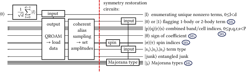
Figure 3: PREPARE operator for the Bloch basis algorithm. In addition to the PREPARE operator of the original sparse qubitization (see Fig 2), it has Majorana type indices that are used by SELECT to apply the correct Majorana types for the Majorana string described by a product state. $j_{t}=0,1$ and $t=1,2,3,4$ enumerates the positions of the Majorana operators in a Majorana string. The circuit for Majorana type symmetry restoration is given in the circuit (LABEL:eq:maj_type_restore_circuit); its input qubits must be loaded by QROAM. The spin symmetry restoration circuit is given in circuit (LABEL:eq:spin_restore_circuit). The Hamiltonian has been written such that no 4-fold or 8-fold symmetry is present any more (see Sec. III.1.3). To simplify the sketch we have depicted that both spin qubits are loaded by QROAM (See the circuit (LABEL:eq:spin_restore_table) for details).

The LCU has multiple repeated coefficients for different values of $j_{1},\dots,j_{4}$ of the Majorana type indices, up to signs like $(-1)^{j_{1}+j_{4}}$. Rather than repeatedly loading the same coefficient with a different sign multiple times, we restore the Majorana type in PREPARE with the following symmetry restoration circuit:

(71)