Medical Image Retrieval via Nearest Neighbor Search on Pre-trained Image Features

Abstract

Nearest neighbor search (NNS) aims to locate the points in high-dimensional space that is closest to the query point. The brute-force approach for finding the nearest neighbor becomes computationally infeasible when the number of points is large. The NNS has multiple applications in medicine, such as searching large medical imaging databases, disease classification, and diagnosis. With a focus on medical imaging, this paper proposes DenseLinkSearch an effective and efficient algorithm that searches and retrieves the relevant images from heterogeneous sources of medical images. Towards this, given a medical database, the proposed algorithm builds an index that consists of pre-computed links of each point in the database. The search algorithm utilizes the index to efficiently traverse the database in search of the nearest neighbor. We extensively tested the proposed NNS approach and compared the performance with state-of-the-art NNS approaches on benchmark datasets and our created medical image datasets. The proposed approach outperformed the existing approaches in terms of retrieving accurate neighbors and retrieval speed. We also explore the role of medical image feature representation in content-based medical image retrieval tasks. We propose a Transformer-based feature representation technique that outperformed the existing pre-trained Transformer-based approaches on CLEF 2011 medical image retrieval task. The source code and datasets of our experiments are available at https://github.com/deepaknlp/DLS.

1 Introduction

Over the past few decades, medical imaging has significantly improved healthcare services. Medical imaging helps to save lives, increase life expectancy, lower mortality rates, reduce the need for exploratory surgery, and shorten hospital stays. With medical imaging, the physician makes better medical decisions regarding diagnosis and treatment. Medical imaging procedures are non-invasive and painless and often do not necessitate any particular preparation beforehand. With the growing demand for medical imaging, the workload of radiologists has increased significantly over the past decades. Mayo Clinic has observed a ten-fold increase in the demand for radiology imaging from just over $9$ million in $1999$ to more than $94$ million in $2010$ [64]. To meet the growing demand, radiologists must process one image every three to four seconds [64]. Consequently, the increase in workload may lead to the incorrect interpretation of the radiology images and compromise the quality and safety of patient care.

The recent advancement in the Artificial intelligence (AI) fields of computer vision and machine learning has the potential to quickly interpret and analyze different forms of medical images [53, 35, 98] and videos [33, 34]. Content-based image retrieval (CBIR) is one of the key tasks in analyzing medical images. It involves indexing the large-scale medical-image datasets and retrieving visually similar images from the existing datasets. With an efficient CBIR system, one can browse, search, and retrieve from the databases images that are visually similar to the query image.

CBIR systems are used to support cancer diagnosis [91, 12], diagnosis of infectious diseases [103] and analyze the central nervous system [65, 19, 57], biomedical image archive [2], malaria parasite detection [52, 79, 51]. Given the growing size of the medical imaging databases, efficiently finding the relevant images is still an important issue to address. Consider a large-scale medical imaging database with hundreds of thousands to millions of medical images, in which each image is represented by high-dimensional (thousands of features) dense vectors. Searching over the millions of images in such high-dimensional space requires an efficient search. The features used to represent the image are another key aspect that affects the image search results. Image features with reduced expressive ability often fail to discriminate the images with the near-similar visual appearance. The role of image features becomes more prominent with image search applications that search over millions of images and demand a higher degree of precision. To address the aforementioned challenges, we focus on developing an algorithm that can efficiently search over millions of medical images. We also examine the role of image features in obtaining relevant and similar images from large-scale medical imaging datasets.

This study presents DenseLinkSearch an efficient algorithm to search and retrieve the relevant images from the heterogeneous sources of medical images and nearest neighbor search benchmark datasets. We first index the feature vectors of the images. The indexing produces a graph with feature vectors as vertices and euclidean distance between the endpoints vectors as edges. In the literature, the tree-based data structure has been used to build indexes to speed up search retrieval. Beygelzimer et al. [8] proposed Cover Tree that was specifically designed to facilitate the speed up of the nearest neighbor search by efficiently building the index. We compare our proposed DenseLinkSearch with the existing tree-based and approximate nearest neighbor approaches and provide a detailed quantitative analysis.

To evaluate the proposed DenseLinkSearch algorithm, we collected $12,851,263$ medical images from the Open biomedical search engine. We extend our experiments on $11$ benchmarked NNS datasets (Artificial, Faces, Corel, MNIST, FMNIST, TinyImages, CovType, Twitter, YearPred, SIFT, and GIST). The experimental results show that our proposed DenseLinkSearch is more efficient and accurate in finding the nearest neighbors in comparison to the existing approaches.

We summarize the contributions of our study as follows:

1. We devise a robust nearest neighbor search algorithm DenseLinkSearch to efficiently search large-scale datasets in which the data points are often represented by the high dimension vectors. To perform the search, we develop an indexing technique that processes the dataset and builds a graph to store the link information of each data point present in the dataset. The created graph in the form of an index is used to quickly scan over the millions of data points in search of the nearest neighbors of the query data point.

2. We also perform an extensive study on the role of features that are used to represent medical images in the dataset. To assess the effectiveness of the features in retrieving the relevant images, we explore multiple deep neural-based features such as ResNet, ViT, and ConvNeXt and analyze their effectiveness in accurately representing the images in high-dimensional spaces.

3. We demonstrate the effectiveness of our proposed DenseLinkSearch on newly created Open medical imaging datasets and eleven other benchmarked NNS datasets. The results show that our proposed NNS technique accurately searches the nearest neighbor orders of magnitude faster than any comparable algorithm.

2 Related Work

2.1 Content-based Image Retrieval

Content-based image retrieval focuses on retrieving images by considering the visual content of the image, such as color, texture, shape, size, intensity, location, etc. For the instance of medical image retrieval, Xue et al. [95] introduced the CervigramFinder system that operates on cervicographic images and aims to find similar images in the database as per the user-defined region. The system extracted color, texture, and size as the visual features. Antani et al. [3] developed SPIRS-IRMA that combines the capability of IRMA [55] system (global image data) and SPIRS [40] system (local region-of-interest image data) to facilitate retrieval based not only on the whole image but also on local image features so that users can retrieve images that are not only similar in terms of their overall appearance but also similar in terms of the pathology that is displayed locally. Depeursinge et al. [24] proposed a 3D localization system based on lung anatomy that is used to localize low-level features used for CBIR. The image retrieval task of the Conference and Labs of the Evaluation Forum (ImageCLEF) has organized multiple medical image retrieval tasks [18, 67, 49, 66] from the year 2004 to 2013. ImageCLEF has provided a venue for the researcher to present their findings and engage in head-to-head comparisons of the efficiency of their medical image retrieval strategies. Over the years, the participants at ImageCLEF made use of a diverse selection of local and global textural features. These included the Tamura features: coarseness, contrast, directionality, line-likeness, regularity, and roughness. Multiple filters such as Gabor, Haar, and Gaussian filters have been used to generate a diverse set of visual features. The visual features [48] for medical image retrieval are also generated using Haralick’s co-occurrence matrix and fractal dimensions.

Rahman et al. [77] proposed a content-based image retrieval framework that deals with the diverse collections of medical images of different modalities, anatomical regions, acquisition views, and biological systems. They extracted the low-level image features such as MPEG (Moving Picture Experts Group)-7 based Edge Histogram Descriptor (EHD) and Color Layout Descriptor (CLD) to represent the images. Further, Rahman et al. [76] presents an image retrieval framework based on image filtering and image similarity fusion. The framework utilizes the support vector machine (SVM) [20] to predict the category of query images and images stored in the database. In this way, the irrelevant images are filtered out, which leads to reduced search space for image similarity matching. A three-stage approach for human brain magnetic resonance image retrieval was introduced by Nazari & Fatemizadeh [68]. In the first stage, the gray level co-occurrence matrix (GLCM) [36] was constructed thereafter, the image features were extracted by computing Features Energy, Entropy, Contrast, Inverse Difference Moment, Variance, Sum Average, Sum Entropy, Sum Variance, Difference Variance, Difference Entropy, and Information measure of correlation. Principal component analysis (PCA) was used for feature reduction in the second stage. An SVM classifier was used in the last stage to perform decision-making.

With the success of the convolution neural network (CNN) for image classification, CNN-based pre-trained models [85, 37, 41, 88, 87] became the de-facto architecture for image classification, feature extraction, and analysis. Qayyum et al. [74] proposed a deep learning-based framework for medical image retrieval tasks. A deep convolutional neural network was trained for the medical image classification, and the trained model was used to extract the image features. Cao et al. [15] developed a deep Boltzmann machine-based multimodal learning model for fusion of the visual and textual information. The proposed multimodal approach enabled searches of the most relevant images for a given image query.

Off-the-shelf pre-trained language models were used to extract the image features for the open domain [16]. The straightforward approach [84, 31, 6] is to extract the image features from the last fully-connected layer; however, it may include irrelevant patterns or background clutter. In another strategy [100, 80, 61], the image features are extracted from convolutional layers that preserve more structural details. In order to extract global and local features for the images, the layer-level [25, 14, 99, 102] feature fusion mechanism has been adapted to complement each feature for the image retrieval task.

2.2 Nearest Neighbor Search

In the course of the last several decades, numerous optimization strategies that are aimed at speeding up the nearest neighbor search have been presented. The tree-based methods have been widely used to speed up the NNS process. In the tree-based approach, a tree-like data structure is used to organize the data points in such a way that it can be efficiently traversed in search of the nearest neighbors for the input query. In general, once the tree structure has been built, the triangle inequality is used to filter the nodes of the tree that can not be the nearest neighbor, thereby reducing the computation and speeding-up the search process. Friedman et al. [29] proposed the first space-partitioning tree KD Tree that uses a depth-first tree traversal technique, followed by backtracking to locate the nearest neighbor in logarithmic time. At each node of KD Tree, $d$-dimensional data points are recursively partitioned into two sets by splitting along one dimension of the data. The split value is often determined to be the median value along the dimension being split. This leads to the points being evenly distributed over the axis-aligned hyper-rectangles. Choosing the split value and split dimensions are the key challenges in KD Tree. To alleviate these issues, Ball Tree [30, 69] was proposed that considered the hyper-spheres instead of hyper-rectangles that form a cluster of the data points in high-dimensional spaces. The Ball Tree computes the centroid of the whole data set, which is then used to recursively partition the data set into two subgroups. It uses triangle inequality to prune the ball and all data points within the ball while searching for nearest neighbors. Other tree-based approaches such as PCA Tree, [86], VP Tree [97], M Tree [17], R Tree [50], and Cover Tree [8] have been introduced in the literature of nearest neighbour search. Most of the tree-based methods for nearest-neighbor search are often well-suited for low dimensional data points, however, they perform poorly in high dimensional spaces.

Wang [90] observed that the performance of tree-based methods is considered to be satisfactory if the search for nearest neighbors requires only a few nodes at each level of the tree. However, in the case of high dimensional data, these approaches lose their effectiveness as the histograms of distances and 1-Lipschitz function values become concentrated [72, 11]. In this case, indexes built with a clustering-based partition technique seem to perform better than the tree-based indexes. By following the clustering-based partition scheme, numerous approaches [73, 90, 1] have been proposed to find the nearest neighbors in high dimensional spaces. In clustering-based indexes, the data points form multiple clusters. While searching for the nearest neighbors, the triangle inequality can be applied to prune the clusters that can’t hold the nearest neighbors.

In another line of research, lower bound-based methods for efficient nearest neighbor search have been proposed. The key idea of the lower bound-based methods is to reduce the distance computation between the query and the candidate data points, which leads to an efficient NNS. Liu et al. [58] proposed two lower bounds: progressive lower bound (PLB) and statistical lower bound (SLB), that aim to reduce the distance computation and accelerate the approximate NNS of the HNSW indexing method [62]. Hwang et al. [43] consider the mean and variance of data points to derive the lower bounds that significantly reduce the distance computations. Further, Hwang et al. [42] introduced product quantized translation that aims to eliminate nearest neighbor candidates effectively using their euclidean distance lower bounds in nonlinear embedded spaces. Jeong et al. [46], Li et al. [56] also utilized the lower bounds strategy to reduce the distance computations. Recently, Zhang et al. [101] introduced the concept of block vectors based on lower bounds that reduce the expensive distance computation. Further, they designed a multilevel lower bound that computes the lower bound step-by-step and makes use of the multistep filtering technique to speed up the search further.

3 Proposed Approach

3.1 Background

In the nearest neighbor search, given a set of $\mathcal{N}$ data points $\mathcal{D}=\{v_{1},v_{2},\ldots,v_{\mathcal{N}}\}$ where $v_{i}\in\mathcal{R}^{d}$, and a distance metric $dist(v_{i},v_{j})$ for points $v_{i}$ and $v_{j}$, for any given query point $q\in\mathcal{R}^{d}$, the goal is to find the nearest point $v^{*}$ in the data points such that:

$$v^{*}=\operatorname*{arg\,min}_{v_{i}\in\mathcal{D}}dist(v_{i},q)$$ (1)

A variant of NNS is the $k$-nearest neighbors (kNN) problem, which aims to find the $k$ nearest points in $\mathcal{D}$ to query $q$, where $k$ is a constant. A brute-force algorithm requires computing the distance between a query point $q$ and each data point in $\mathcal{D}$, resulting in $\mathcal{O}(\mathcal{N})$ time. In applications where the number of points is large, and each data point is high dimensional, it is not computationally feasible to use the brute-force algorithm. Therefore, our goal is to process the data points in advance, which can reduce the computational complexity and quickly find the nearest neighbors of the queries.

3.2 Nearest Neighbor Search

We propose an effective approach to finding the kNN in high-dimensional vector space. The approach deals with building the index and finding the nearest neighbors to the given query with a time-efficient DenseLinkSearch algorithm. In this section, we describe the indexing algorithm and DenseLinkSearch algorithm in detail.

3.2.1 Summary of the Approach

Given a high-dimensional dataset, our proposed approach first builds the index considering all the data points from the dataset. Formally, the indexing algorithm builds the descend and spread links (to be introduced shortly) for each data point by considering the $\mathcal{K}_{index}$ nearest neighbors to them. We use the notation $\mathcal{K}_{index}$ to indicate the number of nearest neighbors embedded in the index. In the indexing process, each vertex forms links to the other vertices, making a cluster of the links that appear to be dense links. While searching for the neighbors nearest to a query after the index is built, DenseLinkSearch algorithm follows the two-stage approach. In the first stage, it follows the descend links of the closest indexed vector to the query vector, and in the second stage, it follows the spread links of the closest indexed vector to surround the query vector. While searching the neighbors, the algorithm spends the majority of the calculation time in the spread stage to find the $\mathcal{K}_{search}$ nearest neighbors. We use the notation $\mathcal{K}_{search}$ to indicate the number of nearest neighbors to the query image that has to be searched in the dataset.

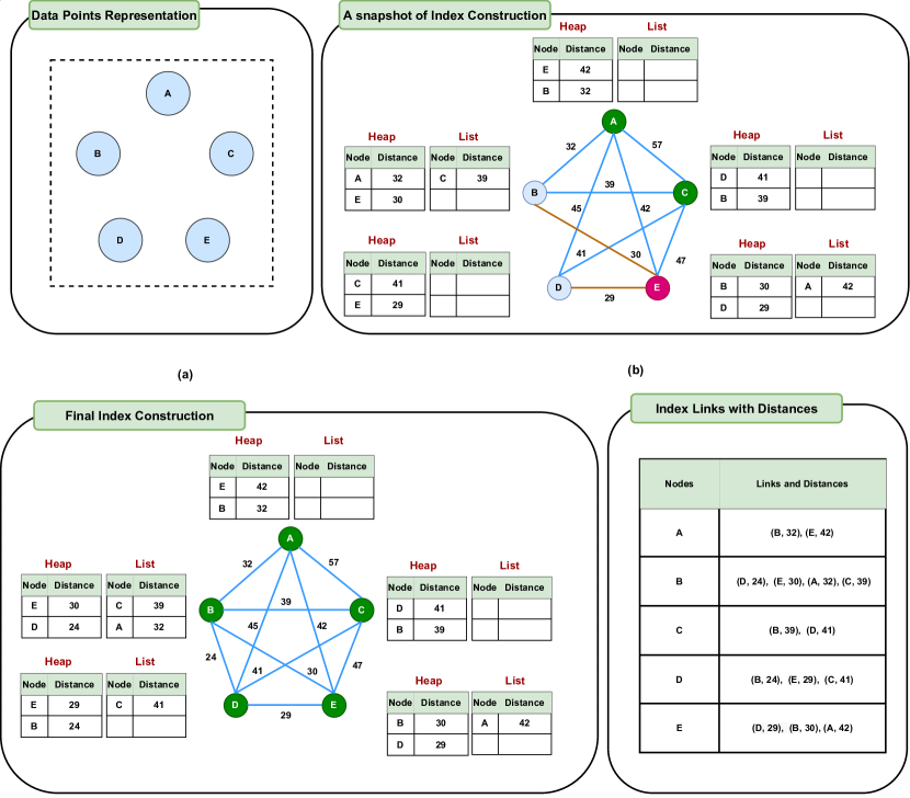
Figure 1: Illustration of the indexing algorithm. Subfigure (a) demonstrates the image vector representation in high-dimensional space. The indexing algorithm considers each vector representation as a vertex and the distance between them as the edge of the index graph. The indexing starts with a random vertex and calls the vertex a node. At any point of time during index construction, a vector representation that has not become a node of the index graph is shown as . The algorithm initializes a heap data structure of size $\mathcal{K}_{index}=2$ and a list. The heap holds links to the nearest vectors known so far. The list holds links to other vectors that consider this vector near. The top link in a heap defines the neighborhood radius, also known as the near distance. Subfigure (b) represents a snapshot of the index after the data point E became a node, and its heap and list are updated based on distances between the node and its neighbors. The existing nodes and edges are shown as and respectively. The recently processed node E and added edges are shown as and respectively. Subfigure (c) demonstrates each node’s heap and list items and the index graph with nodes and edges after the index is built. The created links and distances are shown in subfigure (d). The final index contains the descend and spread links for each node in the dataset. The descend links contain the endpoints vertices and distances from the heap just before the vertex becomes a node while building the indexes. Similarly, the spread links of a given vertex store the endpoints vertices and distances from the heap and list once the algorithm ends.

3.2.2 Indexing Algorithm

Given a dataset $\mathcal{D}$ having $\mathcal{N}$ vectors, the algorithm builds the index by considering the $\mathcal{K}_{index}$ nearest neighbors for each vector in the data. The indexing algorithm constructs an index graph $\mathcal{G}$ where the vertices of the graph are the vectors, and the edges between them hold the Euclidean distances between the two vertices of the graph. The vectors are added to the index one by one. Once the vector is added to the index, it is called a node (vertex), so all nodes are vectors. During indexing, each vector has a spherical neighborhood that encloses neighboring vectors. Neighborhoods contract from infinity (the entire set of data points) at the start of indexing to just the nearest neighbors at the end. When a vector becomes a node, its final neighborhood (the $\mathcal{K}_{index}$ nearest neighbors) is calculated, so its neighborhood shrinks to a minimum. In this process, links are created to neighbors, often causing their neighborhoods to shrink a little as well. Initially, all neighborhoods are huge and overlap, so links are created to all nodes. Later on, neighborhoods overlap with fewer and fewer other neighborhoods, creating fewer links. Shrinking neighborhoods allows indexing to occur with much less than $\mathcal{O}(\mathcal{N}^{2})$ distance calculations.

Variable	Description
$\mathcal{R}_{v}$	Neighborhood radius, also known as near distance.
$\mathcal{C}_{v}$	Distance to closest indexed vector.
$\mathcal{H}_{v}$	Heap to hold the links to the near neighbors of vector $v$. The top of the heap $\mathcal{H}_{v}$ is the link to the furthest of the near neighbor vector.
$\mathcal{L}_{v}$	List to hold the links to the far neighbors of vector $v$. This list hold links to other vectors that consider this vector near.
$\mathcal{I}_{v}$	List to hold finished index links for vector $v$.

Table 1: Description of the variables for each vector $v\in\mathcal{D}$ .

The proposed indexing algorithm has the following steps to build the index:

1. Initialization: For each vector $v$ in the dataset $\mathcal{D}$, we initialize the variables listed in Table 1. We also initialize a global max-heap $\mathcal{H}$ of size $\mathcal{N}$ that stores the distance of the vector that is furthest from all previous indexed nodes at any point of time throughout the indexing process. To hold the final index, we initialize a list $\mathcal{I}$ that stores the list of links $\mathcal{I}_{v}$ for each vector $v$ in the dataset $\mathcal{D}$.

2. Link Creation: To start the indexing, we choose a random vector from the dataset that will become a node of the graph $\mathcal{G}$. The heap $\mathcal{H}$ tracks the nearest known distance $\mathcal{C}_{v}$, for all unindexed vectors. The top of the heap $\mathcal{H}$ is the vector that is the furthest from all indexed nodes. This vector is known as the create vector and will become the next node in the indexing process. The distance from the create vector to the nearest node is known as the create distance. When a vector becomes a node, it is removed from the heap $\mathcal{H}$, and we also copy all the links from the local heap $\mathcal{H}_{v}$ of the vector $v$ and add them into the list $\mathcal{I}_{v}$. The stored links are long at the beginning of indexing, get shorter as indexing progresses, and provide a multiply connected network of links at all length scales for moving around the dataset in descend stage of the DenseLinkSearch.

   During the search, this network of links makes it possible to descend from the root node to a node close to the query vector in $\mathcal{O}(log~{}\mathcal{N})$ steps. These network links are called descend links.

   For a vector $v$, the near distance is defined by the link at the top of the local heap $\mathcal{H}_{v}$, which is the distance to the furthest of the $\mathcal{K}_{index}$ nearest neighbors linked so far. If the heap is not yet full, the near distance is infinite. A vector $\mathcal{A}$ considers another vector $\mathcal{B}$ near if the vector $\mathcal{B}$ is within the vector $\mathcal{A}$’s near distance $\mathcal{R_{A}}$ (also known as neighborhood radius). Since vectors have different neighborhood radii, it is often the case that a vector $\mathcal{A}$ considers a vector $\mathcal{B}$ near, but the vector $\mathcal{B}$ does not consider the vector $\mathcal{A}$ near. For the first $\mathcal{K}_{index}$ nodes indexed, no vector’s heaps are full, and every vector considers every other vector near. Further indexing adds links to vector heaps, pushing out the longest and therefore shrinking the near distance. When neighborhoods shrink to the point that both ends of a link no longer consider the other end near, the link is dropped from the vectors’ heaps and lists.

   Further, to create the links for the new node, we search for the potential neighbors that are not yet nodes, i.e., not yet indexed. A link between vectors $\mathcal{A}$ & $\mathcal{B}$ will only be created if one or both of the vectors consider the other one near. The new link is added to heap $\mathcal{H_{A}}$ of vector $\mathcal{A}$ if vector $\mathcal{A}$ considers vector $\mathcal{B}$ near, i.e., the distance $d_{\mathcal{A},\mathcal{B}}<\mathcal{R_{A}}$, otherwise to list $\mathcal{L_{A}}$ of vector $\mathcal{A}$. Likewise, it is added to heap $\mathcal{H_{B}}$ of vector $\mathcal{B}$ if vector $\mathcal{B}$ considers vector $\mathcal{A}$ near, i.e., the distance $d_{\mathcal{A},\mathcal{B}}<\mathcal{R_{B}}$, otherwise to list $\mathcal{L_{B}}$ of vector $\mathcal{B}$. Adding a link to a full heap will push the top vector out, shrinking the near distance, $\mathcal{R_{A}}$ The link that is pushed out is moved to the list if the other endpoint vector still considers this one near. If neither endpoint considers the other near, the link is dropped.

   When a vector becomes a node, all $\mathcal{K}_{index}$ of its existing descend links are to existing nodes. Due to the node creation order enforced by the global heap $\mathcal{H}$, the early nodes will have long existing links to far away nodes. Creation always chooses the vector that is the furthest away from all existing nodes so that create distance will continually shrink. Therefore, the nodes created later in the indexing process will have mid-range links to nearer nodes. And the last nodes created will have short links to nearest neighbors.

3. Post-processing : At the end of indexing, all nodes have $\mathcal{K}_{index}$ links to their nearest neighbors. These nearest neighbor links are also stored, providing a dense mesh of short links between nearest neighbors. These mesh links make it possible to spread out from a close node to a given query vector and find all the query’s nearest neighbors. These mesh links are called spread links. The same link may be both a descend and spread link, and no real distinction is made during the search. At the end of indexing, all links are unique and sorted by length to optimize the search.

We have illustrated the indexing algorithm with a running example in Fig. 1 and provided the detailed pseudocode for the indexing algorithm in Appendix.

3.2.3 DenseLinkSearch Algorithm

Given the dataset $\mathcal{D}$ with $\mathcal{N}$ vectors and its index containing links $\mathcal{I}$, the DenseLinkSearch algorithm finds the $\mathcal{K}_{search}$ nearest neighbors to the query vector $q$ using the following steps:

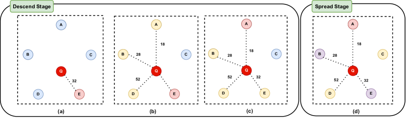
Figure 2: The demonstration of DenseLinkSearch that utilizes the index built as shown in Fig. 1. The DenseLinkSearch operates on the Descend and Spread stages to find the $\mathcal{K}_{search}$ nearest neighbors. The input to the search algorithm is a query vector and the pre-built index with the links. In the subfigure (a), the search starts with a random node (here ) and uses the links of the node to compute the distance between the query vector and the node listed in the links of . In each step of the Descend stage, the algorithm keeps track of the closest vector to the query. Also, a heap $\mathcal{H}$ of size $\mathcal{K}_{search}$ is maintained to track $\mathcal{K}_{search}$ nearest neighbors throughout the search process. In the subfigure (b), the distance between the query vector and the links ( , , and ) of are computed, and the closest vector is updated accordingly. The subfigure (c) shows that the closest node is chosen for the next stage of the Descend. Since the distances ($23$ and $32$) between the query and the links of the node are greater than distance ($18$) between query and node , the search switches to the Spread stage. The Spread stage is demonstrated in subfigure (d), where, we aim to compute the distance between the query and the links ( and ) of node , those have already been computed. At the end of the algorithm, the $\mathcal{K}_{search}$ nearest neighbors can be found in the heap $\mathcal{H}$.

1. Initialization: Firstly, we initialize a global lookup table ${L}$ that stores the vector $v\in\mathcal{D}$ as key and distance $d_{v,q}$ between vector $v$ and query vector $q$ as the value. We also initialize the global heap $\mathcal{H}$ of size $\mathcal{K}_{search}$ to hold $\mathcal{K}_{search}$ nearest neighbors to the query vector $q$. We start the search from the root vector of the dataset $\mathcal{D}$ and compute the distance between the root vector of dataset $\mathcal{D}$ and the query vector. Initially, the root vector is the nearest neighbor to the query; therefore, the vector is pushed into the global heap $\mathcal{H}$ and also recorded into the ${L}$. We also initialize two global variables $\mathcal{V}_{C}$ and ${D}_{C}$. The $\mathcal{V}_{C}$ and ${D}_{C}$ are used to keep track of the nearest vector and closest distance (to the query vector) found at any point of time during the NNS.

2. Descend Stage: The descend stage utilizes the index $\mathcal{I}$ that is built during the indexing process. During the search, we start with the closest vector $\mathcal{V}_{C}$ and retrieve all the links $\mathcal{L}$ of $\mathcal{V}_{C}$ from the $\mathcal{I}$. We traverse each link $l\in\mathcal{L}$, and compute the distance between the vector associated with link $l$ and query vector $q$. During the traversal of the link, we find the local nearest vector and nearest distance from the $\mathcal{L}$ and update the global $\mathcal{V}_{C}$ and ${D}_{C}$. We repeat the Descend step as long as we keep getting closer to the query (the closest distance keeps shrinking). Then, we switch to the Spread stage.

3. Spread Stage: In the Spread stage, we traverse the global heap $\mathcal{H}$ to find the closest vector and its distance to the query vector $q$. Specifically, for each vector $v\in\mathcal{H}$, we extracted their links $\mathcal{L}$ from $\mathcal{L}$ and traverse each link $l\in\mathcal{L}$ in search of the closest vector to the query vector $q$. We continue traversing $\mathcal{H}$ until we find the new closest vector $\mathcal{V}_{N}$ for which the distance ${D}_{N}$ is smaller than the maximum distanced ($\mathcal{D}_{L}$) vector ($\mathcal{V}_{L}$) recorded in the $\mathcal{H}$. Once, we find the closest vector $\mathcal{V}_{N}$ with their distance to query $D_{N}$, we compare the $D_{N}$ with the global closest distance $D_{C}$. In this case, if the $D_{N}$ is smaller than the $D_{C}$ then we update the global closest vector $\mathcal{V}_{C}$ and closet distance $D_{C}$ and perform the Descend stage. Otherwise, if the the $D_{N}$ is smaller than the $D_{L}$ then we perform the Spread stage again.

We have illustrated the DenseLinkSearch algorithm with a running example in Fig. 2 and provided the detailed pseudocode for the DenseLinkSearch algorithm in Appendix.

3.3 Image Feature Representation

To examine the effectiveness of the image feature representation, we performed an extensive experiment considering multiple feature extraction models. We also explore the different feature aggregation techniques to assess their significance in image-based retrieval. In this section, we discuss the feature extraction models and feature aggregators in detail.

3.3.1 Medical Image Feature Extractors

1. Deep Residual Network: Gradient degradation is a key challenge in training deep neural networks. It is the issue of an increase in training error when layers get added to the network. This causes the low accuracy of the neural network model. With the increase in layers of the network, the gradient computed in the back-propagation step starts to diminish. This problem of vanishing derivatives in deep neural networks is called vanishing gradient descent [39]. To overcome these problems, He et al. [37], introduced a deep residual learning framework with deep convolutional neural networks (CNNs) that reformulate the layers as learning residual functions with reference to the layer inputs instead of learning unreferenced functions. Given the input $x$ received from the previous layer, the residual learning framework, the original mapping is recast into $\mathcal{F}(x)+x$. The formulation of $\mathcal{F}(x)+x$ can be realized by feedforward neural networks with “shortcut connections”. These connections perform identity mapping, and the outputs of connections are summed to the stacked layers’ outputs. In this study, we utilize the pre-trained ResNet50 model as a feature extractor.

2. Vision Transformers: Inspired by the success of Transformer architecture [89] in Natural Language Processing (NLP), Dosovitskiy et al. [27] explore the Transformer architecture with the images and develop Vision Transformer (ViT) . With the Transformer, the images are treated like tokens, as in NLP, by splitting the images into patches. The patch embedding is added with position embedding and passed as input to the Transformer layer. The study conducted by Dosovitskiy et al. [27] shows that Transformer applied directly to sequences of image patches achieved better results on image classification tasks compared to the CNNs while using fewer computational resources to train the model. We utilize the pre-trained ViT-Base, ViT-Large and ViT-Huge models as image feature extractors.

3. ConvNeXt: The ConvNeXt [60] is a family of pure CNNs, which is developed by considering the multiple design decisions in Transformers. The ConvNeXt family considers the following key design decisions:

   1. The ConvNeXt follows the Swin Transformers [59] stage compute ratio strategy. To adopt the strategy, it adjusts the number of blocks sampled in each stage of the network from ($3,4,6,3$) in ResNet50 to ($3,3,9,3$) in ConvNeXt.

   2. The ConvNeXt adopted the grouped convolution approach of ResNeXt [94] and uses depth-wise convolution, a special case of grouped convolution where the number of groups equals the number of channels.

   3. The ConvNeXt considers the larger kernel-size convolution operations. Varying the kernel sizes from $3$ to $11$, they found the optimal kernel size of $7\times 7$.

   4. Additionally, ConvNeXt replaces the ReLU activation with the fewer GELU [38] activation functions and fewer batch normalization [83] layers.

In this work, we utilized pre-trained ConvNeXt-B, ConvNeXt-L, and ConvNeXt-XL as image feature extractors.

3.3.2 Feature Aggregations

Given an image $\mathcal{M}$ and an image feature extractor $\mathcal{G}(\mathcal{M};\theta)$, where $\theta$ denotes the feature extractor parameters that are frozen during feature extraction, we first pre-process the image and transform the image $\mathcal{M}$ into $\mathcal{X}\in\mathcal{R}^{c\times w\times h}$, where $c$, $w$ and $h$ are number of channels, width, and height of the image respectively. The feature extractor $\mathcal{G}$ takes $\mathcal{X}$ as input and produces the 3D tensor $x\in\mathcal{R}^{K\times W\times H}$, where $K$ is the number of feature maps in the last layer of feature extractor, $W$ and $H$ refers to the width and height of the feature map respectively.

1. Max Pooling: In max pooling, the maximum value of the spatial feature activation for each feature map is considered for feature representation. Formally,

   $$f^{(max)}=[f_{1}^{(max)},f_{2}^{(max)},\ldots f_{K}^{(max)}]^{\top}$$ (2)

   where $f_{k}^{(max)}=max_{y\in x_{k}}(y)$ is the value obtained after applying $max$ operation on $k^{th}$ feature map $x_{k}\in\mathcal{R}^{W\times H}$.

2. Sum Pooling: The sum pooling aims to obtain the feature representation by summing the value of the spatial feature activation for each. Formally,

   $$f^{(sum)}=[f_{1}^{(sum)},f_{2}^{(sum)},\ldots f_{K}^{(sum)}]^{\top}$$ (3)

   where $f_{k}^{(sum)}=sum_{y\in x_{k}}(y)$ is the value obtained after applying $sum$ operation on $k^{th}$ feature map $x_{k}\in\mathcal{R}^{W\times H}$.

3. Mean Pooling: In mean pooling, the average value of the spatial feature activation for each feature map is considered for feature representation. Formally,

   $$f^{(mean)}=[f_{1}^{(mean)},f_{2}^{(mean)},\ldots f_{K}^{(mean)}]^{\top}$$ (4)

   where $f_{k}^{(mean)}=mean_{y\in x_{k}}(y)$ is the value obtained after applying $mean$ operation on $k^{th}$ feature map $x_{k}\in\mathcal{R}^{W\times H}$.

4. Generalized Mean Pooling: It is the generalization of the pooling technique where generalized mean [26, 75] is used to derive the pooling function. Formally,

   $$f^{(gmean)} =[f_{1}^{(gmean)},f_{2}^{(gmean)},\ldots f_{K}^{(gmean)}]^{\top}$$ (5)

   $$\text{where}\quad f_{k}^{(gmean)} =\left(\frac{1}{|x_{k}|}\sum_{y\in x_{k}}\!y^{p_{k}}\right)^{\frac{1}{p_{k}}}$$ (6)

   where $p_{k}$ is a hyper-parameter.

5. Spatial-wise Attention: In spatial-wise attention, we model the importance of each spatial feature by computing the weight. The final feature is generated by considering the spatial weight. We build an attention matrix $\alpha\in\mathcal{R}^{W\times H}$. The sum of any row or column of the matrix $\alpha$ is $1$, which signifies the importance of each spatial position. First, we compute the weight matrix $w\in\mathcal{R}^{W\times H}$, as follows:

   $$w=\sum_{k=1}^{K}y_{k}$$ (7)

   Then we apply the row-wise softmax and column-wise softmax operation on $w$ to obtain the attention matrix $\alpha$. The final aggregated features $f^{spatial}$ are obtained as follows:

   $$f^{(spatial)}=[f_{1}^{(spatial)},f_{2}^{(spatial)},\ldots f_{K}^{(spatial)}]^{\top}$$ (8)

   where $f_{k}^{(spatial)}=mean(x_{k}*\alpha$), obtained after applying element-wise multiplication on $x_{k}$ and $\alpha$. The $mean$ operation is used to aggregate the feature activation.

6. Channel-wise Attention: In the channel-wise attention, we model the importance of each feature map (channel) by computing the weight. The final feature is generated by considering the channel weight. We build an attention matrix $\beta\in\mathcal{R}^{K}$. The sum of each element of $\beta$ is $1$, which signifies the importance of each feature map. Similar to the spatial-wise attention; first, we compute the weight matrix $w\in\mathcal{R}^{K}$, as follows:

   $$w^{k}=\sum_{i=1}^{W}\sum_{j=1}^{H}a_{i,j}^{k}$$ (9)

   where $a_{i,j}^{k}$ is an element of $k^{th}$ feature map. Then we apply the softmax operation on $w$ to obtain the attention matrix $\beta$. The final aggregated features $f^{channel}$ are obtained as follows:

   $$f^{(channel)}=[f_{1}^{(channel)},f_{2}^{(channel)},\ldots f_{K}^{(channel)}]^{\top}$$ (10)

   where $f_{k}^{(channel)}=mean(x_{k}\times\beta$), obtained after applying scalar multiplication on $x_{k}$ with $\beta$. The $mean$ operation is used to aggregate the feature activation.

   For the case of the ConvNeXt feature extractor, we performed a detailed investigation on the ConvNeXt layers. We observe that pre-trained LayerNorm [4] weights from the last convolution layer can be exploited to obtain better feature representation. Therefore, we pool the ConvNeXt features as follows:

   $$\begin{split}f^{(mean)}&=[f_{1}^{(mean)},f_{2}^{(mean)},\ldots f_{K}^{(mean)}]^{\top}\\ f^{(lmean)}&=\text{{LayerNorm}}(\sigma(f^{(mean)}))\\ \end{split}$$ (11)

   where $f_{k}^{(mean)}=mean_{y\in x_{k}}(y)$ is the value obtained after applying $mean$ operation on $k^{th}$ feature map $x_{k}\in\mathcal{R}^{W\times H}$. $\sigma$ denotes the $sigmoid$ activation function. LayerNorm(.) denotes the LayerNorm operation whose weights are initialized with the pre-trained weights from ConvNeXt model.

4 Experimental Setup

This section describes the experimental setups for NNS and medical image feature extractors for image retrieval.

4.1 Nearest Neighbor Search

4.1.1 Index and DenseLinkSearch Computational Details

We ran all the experiments on a computing node having $72$ CPU, $36$ cores, and $256$ GB RAM. The DenseLinkSearch has $\mathcal{K}_{index}$ and $\mathcal{K}_{search}$ as two key hyper-parameters. The former denotes the number of nearest neighbors calculated and kept in the index, while the latter represents the number of nearest neighbors found by DenseLinkSearch during the search. We have provided the best hyper-parameters values for each NNS approaches in Tables 7, and 8 in the Appendix.

4.1.2 Datasets for NNS

We evaluated our NNS approach on multiple benchmark datasets from UCI repository and from the ANN-Benchmark. The datasets are diverse in the number of samples (minimum 10K, maximum 12.85M) as well as the dimensions of the sample (minimum 20, maximum 1536). The datasets MNIST, FMNIST, SIFT, and GIST come with the train and test split; we split the remaining datasets into train and test. We use the training datasets to build the indexes and the test datasets to find the $10$ nearest neighbors for each query. We have provided the details of each dataset along with their size and dimensions in Table 2.

OpenI Datasets

The OpenI datasets comprises images from the Open Access (OA) subset of PubMed Central (PMC). We have curated around $4,222,779$ million articles from PMC OA and extracted $14,908,095$ images from the curated articles. The scientific articles also contain multi-panel images. The multi-panel images are further split into single-panel images using the panel segmentation approach [23] resulting in a total of $24,625,466$ images. These images also contain graphical illustrations such as charts and graphs. We employ our in-house modality detector Rahman et al. [78] that categorizes each image into one of the eight modality classes [78]. We excluded the images that have been predicted as graphical and only considered medical non-graphical images. This process yields $12,851,263$ images. The medical image retrieval task experiments described in Section 5.2 showed that the ConvNeXt-L (IN-22K) model outperforms the existing medical image feature extractors. Therefore, we utilized ConvNeXt-L (IN-22K) to generate the image features for the OpenI dataset and called it the OpenI-ConvNeXt dataset. To assess the role of feature dimensions for the OpenI dataset, we also generated the image features from the ResNet50 model having $512$ dimensions; we call this OpenI-ResNet dataset.

Dataset	# Samples	Dimension	# Build Index	# Query
Artificial [10]	10,000	40	9,000	1,000
Faces [28]	10,304	20	9,304	1,000
Corel [70]	68,040	32	58,040	10,000
MNIST [54]	70,000	784	60,000	10,000
FMNIST [93]	70,000	784	60,000	10,000
TinyImages [28]	100,000	384	90,000	10,000
CovType [9]	581,012	54	571,012	10,000
Twitter [28]	583,250	78	573,250	10,000
YearPred [28]	515,345	90	505,345	10,000
SIFT [45]	1,000,000	128	990,000	10,000
GIST [45]	1,000,000	960	999,000	1,000
OpenI-ResNet (Ours)	12,851,263	512	12,841,263	10,000
OpenI-ConvNeXt (Ours)	12,851,263	1,536	12,841,263	10,000

Table 2: The details of the benchmark and our created OpenI datasets used for the nearest neighbor search experiments.

4.1.3 Evaluation Metrics for NNS

We evaluate the performance of NNS using the following two metrics:

1. Recall@k (R@k): It is the ratio of the true nearest neighbors retrieved in the top-k nearest neighbors by the algorithm to the $k$ true nearest neighbors in the test set. In this study, we focused on retrieving the 10 nearest neighbors; therefore, the metric is R@10.

2. Average time per query (ATPQ): It measures the average time per query taken by NNS approaches to retrieve the 10 nearest neighbors. We report this metric in milliseconds.

4.1.4 Baseline NNS Methods

We compare the performance of our proposed DenseLinkSearch (DLS) approach with the following competitive NNS methods.

1. KD Tree [29] and Ball Tree [30]: These are the tree-based approach used to find the nearest neighbors. We have discussed these approaches in Section 2. We use the scikit-learn [71] implementation of KD and Ball Tree.

2. RP Forest [96]: It works on the concepts of random projection tree [21] where nearest neighbors are found by combining multiple trees with each constructed recursively through a series of random projections. We utilized the rpForest implementation.

3. Facebook Artificial Intelligence Similarity Search (FAISS) : Faiss [47] is an approximate nearest neighbors implementation of Locality Sensitive Hashing (LSH) [22] based indexing, Inverse Vector File (IVF) [5], and Product Quantization [45]. We use the FAISS implementation.

4. Annoy [7]: We utilized the approximate nearest neighbors method Annoy that strives to minimize memory usage.

5. Multiple Random Projection Trees (MRPT) [44]: In MRPT, multiple random projection trees are combined by a voting scheme. The overall idea is to exploit the redundancy in a large number of candidate data points and eventually reduce the number of expensive exact distance computations using independently generated random projections. We utilized the official implementation.

6. Hierarchical Navigable Small World (HNSW) [63]: This is a graph-based approximate nearest neighbor approach. HNSW builds a multi-layer structure consisting of a hierarchical set of proximity graphs for nested subsets of the stored elements. To obtain the results from HNSW, we utilized the official implementation.

7. Scalable Nearest Neighbors (ScaNN) [32]: It is a quantization based nearest search method that computes the approximate distance between each data point and query vector. We utilized the official implementation.

4.2 Medical Image Feature Extractors for Image Retrieval Evaluation

4.2.1 Feature Extractors Details and Hyper-parameters

To extract the features for the images, we use pre-trained weights from the ResNet, ViT, and ConvNeXt models. For the ResNet, we use pre-trained ResNet50 weights. We extracted the features from the conv5_block1_2_conv layer of the ResNet50 model. This layer returns the output tensor of shape $512\times 7\times 7$. For ViT, we experiment with the ViT-Base (dimension 768), ViT-Large (dimension 1024), and ViT-Huge (dimension 1280) models. Since ViT is a Transformer model, the [CLS] token representation is considered as the image feature representation. For the ConvNeXt model, we experiment with the variants of the ConvNeXt models. We mainly experiment with the model variants trained on ImageNet-1K [82] dataset and pre-trained on ImageNet-22K [81] dataset. We experiment with ConvNeXt-B, ConvNeXt-L and ConvNeXt-XL models that output feature map shapes $1024\times 9\times 9$, $1536\times 9\times 9$ and $2048\times 9\times 9$ respectively. We utilized pre-trained weights of ViT and ConvNeXt models from timm [92]. For generalized mean pooling, we set the $p_{k}$ hyper-parameter value as $2$.

4.2.2 Image Retrieval Dataset and evaluation

We used the ImageCLEF 2011 dataset [49].The dataset consists of $231,000$ images from PubMed Central articles, $30$ textual and visual queries, and relevance judgments. For the visual queries, 2-3 sample images (enumerated) are provided. In this study, we used only the first image as visual query to retrieve the relevant images from the pool of $231,000$ images. For each image, we extract the features from the pre-trained models and rank the images based on the cosine similarity between the query image and database image. As in ImageCLEF evaluations, we evaluated the performance using Mean Average Precision, Precision@k, R-precision, and binary preference. The metrics are defined as follows:

1. Precision at k (P@k): Precision at $k$ is the proportion of system retrieved images that are correct.

   $$\text{P@k}=\frac{\text{\# of correctly retrieved images in the top-k}}{\text{\# of retrieved images}}$$ (12)

2. Mean Average Precision (MAP): MAP is the average precision averaged across a set of queries.

   $$\text{MAP}=\frac{1}{|Q|}\sum_{j=1}^{|Q|}\frac{1}{m_{j}}\sum_{k=1}^{m_{j}}P@k_{j}$$ (13)

   where $Q$ is the total set of queries, $m_{j}$ is the number of correct images returned for the $j^{th}$ query.

3. R-precision (Rprec) [13]: It is defined as the precision of the retrieval system after $R$ documents are retrieved where R is the number of relevant images for the given image query.

4. Binary Preference (bpref) [13]: It computes a preference relation of whether judged relevant images are retrieved ahead of judged irrelevant images. It is defined as follows:

   $$\text{bpref}=\frac{1}{R}\sum_{r}(1-\frac{|n~{}\text{ranked higher than}~{}r|}{R})$$ (14)

   Where $N$ and $R$ are the numbers of judged non-relevant and relevant images, respectively. The notation $r$ is a relevant image, and $n$ is a member of the first $R$ judged non-relevant images as retrieved by the system. We use the trec_eval evaluation tool to compute the aforementioned metrics.

5 Results and Discussion

5.1 Nearest Neighbor Search

The detailed results comparing the proposed DLS with tree-based and approximate NNS methods are shown in Tables 3 and 4 respectively. The best-performing FAISS approach on the respective dataset is shown in Table 4, and the performance of the multiple FAISS approaches are shown in Table 9. We have highlighted the FAISS family approach that yield the best performance on the respective dataset in Table 9. To report the results (ATPQ and R@10) using the DLS approach on each dataset, we ran the experiments three times and reported the mean value of the results.

For the Faces dataset, our approach outperformed the most competitive approaches (ScaNN and MRPT) with an Avg value of $0.10$ and an R@10 value of $99.20$. The tree-based approaches also reported the R@10 $\geq 99\%$; however, their ATPQ was very high ($0.216$ for KD Tree and $0.214$ for the Ball Tree). Similarly, for the datasets (MNIST, FMNIST, Corel) having size $\approx 70,000$, our approach outperformed the counterpart NNS approaches. We observe that approximate NNS approaches MRPT and HNSW also reported the competitive R@10 values ($\geq 99\%$) however, the proposed DLS approach has lower ATPQ with $\geq 99\%$ R@10 values on MNIST, FMNIST, and Corel datasets. On the TinyImages (size=$100,000$ and dimension=$384$), our approach reported the ATPQ of $3.7$ ms with an R@10 of $99.10\%$; the closet competitive approach ScaNN reported the ATPQ of $0.649$ ms; however, their R@10 was $98.6\%$. The other competitive approach MRPT obtained the R@10 of $99.99\%$ on the TinyImages dataset; however, their ATPQ was $14.31$ ms.

	Brute Search		KD Tree		Ball Tree		RP Forest		DLS
	ATPQ (ms) $\downarrow$	R@10 (%) $\uparrow$	ATPQ (ms) $\downarrow$	R@10 (%) $\uparrow$	ATPQ (ms) $\downarrow$	R@10 (%) $\uparrow$	ATPQ (ms) $\downarrow$	R@10 (%) $\uparrow$	ATPQ (ms) $\downarrow$	R@10 (%) $\uparrow$
Artificial	0.860	100	0.471	100.0	0.471	100.0	0.776	47.79	0.460	99.30
Faces	0.560	100	0.216	99.98	0.214	99.98	0.934	48.13	0.100	99.20
Corel	4.200	100	2.432	99.99	2.383	99.99	6.880	68.31	0.090	99.50
MNIST	100	100	87.30	100.0	87.24	100.0	31.48	71.74	0.850	99.00
FMNIST	100	100	88.92	100.0	88.70	100.0	38.20	47.17	0.780	99.30
CovType	74.00	100	46.21	99.99	46.14	99.99	40.43	73.93	0.360	99.10
TinyImages	76.00	100	62.93	99.99	63.01	99.99	34.16	35.35	3.700	99.10
Twitter	110.0	100	70.19	99.60	70.06	99.60	78.01	18.68	0.420	99.50
YearPred	120.0	100	74.08	99.99	74.09	99.99	58.48	25.30	2.000	99.30
SIFT	280.0	100	215.4	99.93	216.0	99.93	184.5	99.21	1.600	99.70
GIST	2200	100	1920	99.91	1919	99.91	735.1	35.70	36.00	99.10

Table 3: Comparison of the proposed DLS approach with multiple tree-based nearest neighbors approaches on benchmark datasets. The highlighted cells represent the R@10$\geq 99\%$ for which the ATPQ is the lowest amongst all the approaches. Due to the overhead of memory footprint, we could not run the experiments with tree-based approaches on the OpenI datasets.

	Brute Search		FAISS		Annoy		MRPT		HNSW		ScaNN		DLS
	ATPQ (ms) $\downarrow$	R@10 (%) $\uparrow$	ATPQ (ms) $\downarrow$	R@10 (%) $\uparrow$	ATPQ (ms) $\downarrow$	R@10 (%) $\uparrow$	ATPQ (ms) $\downarrow$	R@10 (%) $\uparrow$	ATPQ (ms) $\downarrow$	R@10 (%) $\uparrow$	ATPQ (ms) $\downarrow$	R@10 (%) $\uparrow$	ATPQ (ms) $\downarrow$	R@10 (%) $\uparrow$
Artificial	0.860	100	3.754	49.63	1.034	99.20	0.123	100.0	0.037	71.39	0.033	96.65	0.460	99.30
Faces	0.560	100	0.044	89.46	0.992	99.41	0.111	99.97	0.019	86.51	0.025	96.66	0.100	99.20
Corel	4.200	100	0.217	90.50	1.306	99.92	0.657	99.99	0.024	96.62	0.078	57.95	0.090	99.50
MNIST	100.0	100	4.683	86.02	2.235	99.29	17.28	100.0	0.124	93.42	0.878	100.0	0.850	99.00
FMNIST	100.0	100	4.986	92.99	2.259	99.06	17.61	100.0	0.119	94.04	0.898	100.0	0.780	99.30
CovType	74.00	100	6.532	99.22	0.575	99.99	15.18	99.99	0.024	98.63	0.081	17.25	0.360	99.10
TinyImages	76.00	100	3.074	73.11	3.692	86.27	14.31	99.99	0.140	63.16	0.649	98.96	3.700	99.10
Twitter	110.0	100	10.19	97.23	2.056	98.81	20.22	98.95	0.051	92.79	0.038	2.228	0.420	99.50
YearPred	120.0	100	7.299	90.48	1.995	97.28	19.50	99.99	0.077	79.95	0.895	5.818	2.000	99.30
SIFT	280.0	100	13.41	89.00	2.542	92.57	51.61	99.92	0.106	79.48	3.625	98.72	1.600	99.70
GIST	2200	100	140.9	78.59	9.081	69.19	368.9	99.89	0.718	54.32	26.21	96.20	36.00	99.10
OpenI-ResNet	19760	100	869.72	85.80	11.96	87.03	2815.4	99.83	1.187	68.74	178.83	98.68	18.92	99.20
OpenI-ConvNeXt	3423	100	2475.7	90.20	18.35	82.23	7993.4	99.48	0.7852	54.32	530.20	99.10	100.2	97.89

Table 4: Comparison of the proposed DLS approach with approximate nearest neighbors approaches on benchmark datasets. The performance of the best approach from the FAISS family approaches on each dataset is reported under FAISS column. FAISS-IVF performed best amongst all the FAISS’s approaches for each dataset except Artificial dataset. Average time per query (ATPQ) is reported in milliseconds, and Recall@10 (R@10) is reported in percentage. The highlighted cells represent the R@10$\geq 99\%$ for which the ATPQ is the lowest amongst all the approaches. The highlighted cells represent the R@10$\geq 97\%$ for which the ATPQ is the lowest amongst all the approaches. Lower ATPQ and higher R@10 are better.

We also analyze the results on the CovType, Twitter, and YearPred datasets, which have the dataset size $\approx 500,000$. For the CovType, our approach has the ATPQ of $0.36$ ms with R@10 of $99.1\%$. The closest NNS approach HNSW, has the ATPQ of $0.024$ with R@10 of $98.63\%$. Another approximate NNS approach, Annoy, also obtained the R@10 of $99.99\%$ with the ATPQ of $0.575$ ms. Our proposed DLS approach obtained the ATPQ of $0.42$ ms with R@10 of $99.5\%$ on the Twitter dataset. The HNSW recorded the AvgTime of $0.051$ with the R@10 of 92.79. We observe similar patterns on the large-scale datasets (SIFT, GIST, OpenI-ResNet, OpenI-ConvNeXt) with the high dimensions and the dataset sizes in the millions. Our approach outperformed the existing competitive approaches on these high-dimension datasets as well. To summarize, the tree-based approaches consistently produced $\geq 99\%$ R@10; however, the AvgTime were high, which makes them unsuitable for real-time applications, where the latency and accuracy both matter equally. In comparison to the approximate NNS approaches, our proposed DLS approach outperformed them in terms of lower AvgTime and $\geq 99\%$ R@10 on 11 out of 13 datasets.

5.1.1 Effect of $\mathcal{K}_{index}$ and $\mathcal{K}_{search}$

To analyze the effect of the hyper-parameters $\mathcal{K}_{index}$ and $\mathcal{K}_{search}$ of our proposed DLS approach, we performed detailed sensitivity analysis on each benchmark dataset with combination of $\mathcal{K}_{index}$ and $\mathcal{K}_{search}$ values. We observed that search speed is slower when $\mathcal{K}_{index}$ increases (i.e., includes more nearest neighbor links in the index), and $\mathcal{K}_{search}$ increases (i.e., finds more nearest neighbors with spread during search). In contrast, the R@10 improves as $\mathcal{K}_{index}$ and $\mathcal{K}_{search}$ increase. Similar patterns were observed throughout all the datasets, which confirms that there is a trade-off between search speed and recall; accordingly $\mathcal{K}_{index}$ and $\mathcal{K}_{search}$ should be chosen for the DLS approach as needed. To perform this sensitivity analysis on the OpenI datasets, we chose a subset of the datasets having a size of $1,000,000$ and chose the combinations of $\mathcal{K}_{index}$ and $\mathcal{K}_{search}$ to perform the analysis. We have provided the chart for both the OpenI datasets in Fig. 3 and 4.

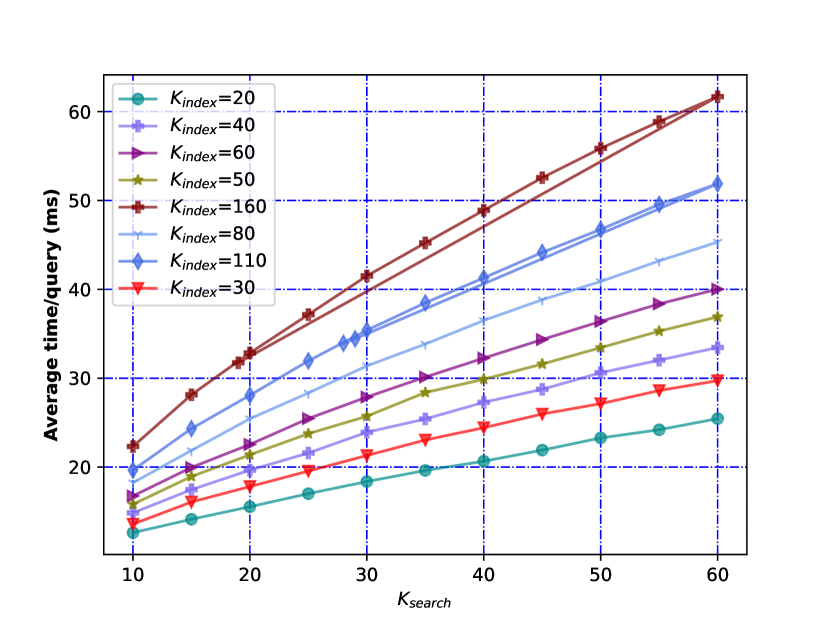
(a)

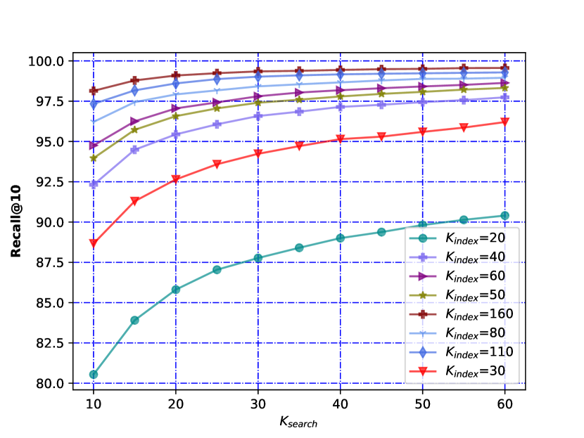
(b)

Figure 3: The effect of $\mathcal{K}_{index}$ and $\mathcal{K}_{search}$ on ATPQ (a) and Recall@10 (b) on 1,000,000 samples of OpenI-ConvNeXt dataset.

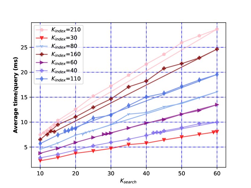
(a)

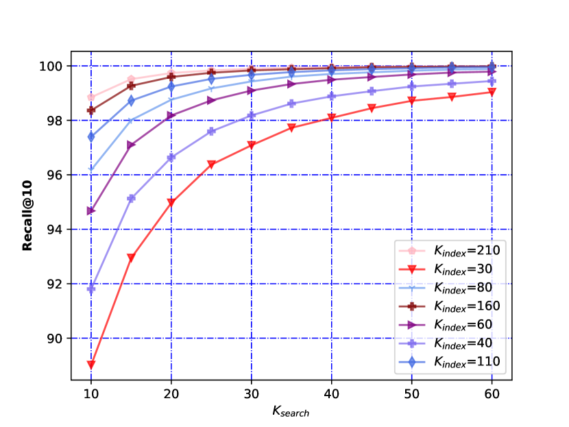
(b)

Figure 4: The effect of $\mathcal{K}_{index}$ and $\mathcal{K}_{search}$ on ATPQ (a) and Recall@10 (b) on 1,000,000 samples of the OpenI-ResNet dataset.

5.1.2 Effect of dataset size and feature dimensions

To understand the effect of the dataset size and feature dimensions on the DLS approach, we performed an in-depth analysis by varying the dataset size from $250K$ to $12.85M$ on the OpenI datasets having feature dimensions $512$ and $1,536$. We observe that the average time per query increases with an increase in dataset size as the algorithm needs to perform more distance computations to retrieve the nearest neighbors. With respect to the increase in feature dimensions from $512$ to $1,536$, we notice that the average time per query increases $2.27$, $3.87$, $4.74$ times on $\mathcal{K}_{search}=10$ for $1M$, $3M$ and $12M$ dataset sizes respectively. We have provided the trends for both the OpenI datasets in Fig. 5 and 6.

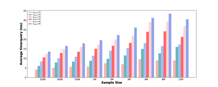
Figure 5: Effect of the sample size on the average time per query for OpenI-ResNet dataset.

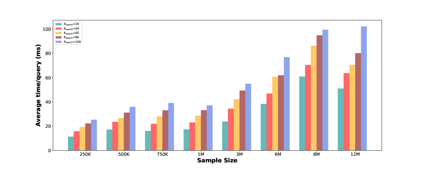
Figure 6: Effect of the sample size on the average time per query for OpenI-ConvNeXt dataset.

5.2 Medical Image Feature Extractors

Table 5) presents the results from multiple feature extractors on the ImageCLEF 2011 medical image retrieval task.

For the ResNet50 model, mean and sum pooling performed better than max pooling on multiple metrics, with a maximum of $0.0518$ and $0.1500$ MAP and P@20 scores using mean pooling with the ResNet50 model. We observed that the ViT-Base model performs better than its counterpart ViT-Large and ViT-Huge models. It achieves the maximum MAP of $0.0713$ compared to the ResNet-Mean, which achieved a MAP score of $0.0518$. The ConvNeXt-L (IN-22K) model achieved the maximum evaluation scores amongst all the variants of ConvNeXt and their counterpart feature extractors. The ConvNeXt-L (IN-22K) model outperformed the best ResNet model by $0.032$, $0.02$, and $0.0674$ in terms of MAP, P@20, and bpref, respectively. It outperformed the best ViT model by $0.0125$, $0.02$, and $0.0126$ in terms of MAP, P@20, and bpref, respectively. Our results are somewhat higher than the best performing system at CLEF 2011 ($0.05$, $0.0533$, and $0.1346$ in terms of MAP, P@10, and bpref, respectively.)

We report the ConvNeXt-L (IN-22K) with mean pooling results (row 1) in Table 6. We aggregated the features with multiple pooling strategies discussed in Section 3.3.2 and report the results in Table 6. We did not observe any improvements with other feature aggregation strategies over the mean pooling. Since the mean pooling operation performed by the ConvNeXt-L model also utilizes the pre-trained LayerNorm parameters, we also performed the experiments with pre-trained LayerNorm parameters. With this approach, we recorded the improvement in terms of multiple evaluation metrics using the Generalized Mean pooling strategy over mean pooling. The Generalized Mean pooling strategy obtained an improvement of $0.0134$, $0.02$, and $0.01$ in terms of P@5, P@10, and P@20, respectively, in comparison to the mean pooling.

Models	MAP	P@5	P@10	P@20	Rprec	bpref
ResNet with Max-pooling	0.0463	0.1733	0.1533	0.1383	0.0841	0.1455
ResNet with Mean-pooling	0.0518	0.2000	0.1900	0.1500	0.0838	0.1479
ResNet with Sum-pooling	0.0517	0.2000	0.1900	0.1500	0.0838	0.1479
ViT-Base	0.0713	0.2133	0.1833	0.1433	0.1109	0.2027
ViT-Large	0.0679	0.1933	0.1833	0.1500	0.0907	0.1934
ViT-Huge	0.0666	0.1600	0.1467	0.1450	0.1146	0.1962
ConvNeXt-B	0.0459	0.1067	0.1033	0.0933	0.0759	0.1595
ConvNeXt-B (IN-22K)	0.0699	0.2133	0.1667	0.1500	0.1037	0.2041
ConvNeXt-L	0.0450	0.1267	0.1133	0.0950	0.0722	0.1568
ConvNeXt-L (IN-22K)	0.0838	0.2333	0.2033	0.1700	0.1186	0.2153
ConvNeXt-XL (IN-22K)	0.0802	0.2067	0.1700	0.1617	0.1091	0.2146
Kalpathy-Cramer et al. [49]	0.0338	–	0.1500	–	–	0.0807

Table 5: Performance comparison on CLEF 2011 dataset on medical image retrieval task. IN-22K refers to the model that is pre-trained on the ImageNet-22K dataset.

Models		MAP	P@5	P@10	P@20	Rprec	bpref
ConvNeXt-L (IN-22K)		0.0838	0.2333	0.2033	0.1700	0.1186	0.2153
Pooling	Max	0.0279	0.1267	0.1067	0.0933	0.0542	0.1290
	Sum	0.0698	0.2000	0.1800	0.1500	0.1033	0.1926
	Spatial-wise Attention	0.0677	0.2133	0.1733	0.1533	0.1024	0.1923
	Channel-wise Attention	0.0002	0.0000	0.0000	0.0000	0.0031	0.0143
	Generalized Mean	0.0521	0.1600	0.1167	0.1117	0.0833	0.1706
LayerNorm with Pooling	Max	0.0289	0.1133	0.1100	0.0900	0.0614	0.1133
	Sum	0.0836	0.2467	0.2133	0.1833	0.1126	0.2100
	Spatial-wise Attention	0.0821	0.2333	0.1967	0.1783	0.1110	0.2086
	Channel-wise Attention	0.0046	0.0200	0.0233	0.0200	0.0162	0.0554
	Generalized Mean	0.0838	0.2467	0.2233	0.1800	0.1153	0.2129

Table 6: Performance comparison of different feature aggregation (pooling) techniques on CLEF 2011 dataset on medical image retrieval task. The feature maps from model ConvNeXt-L (IN-22K) are extracted, and respective pooling operation was performed to report the numbers. The first row results are reported with mean pooling operation.

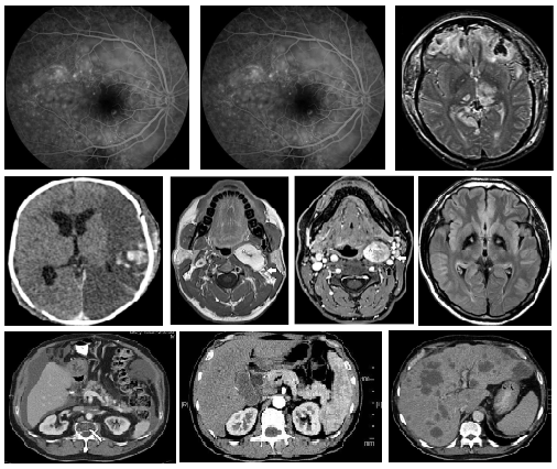
(a)

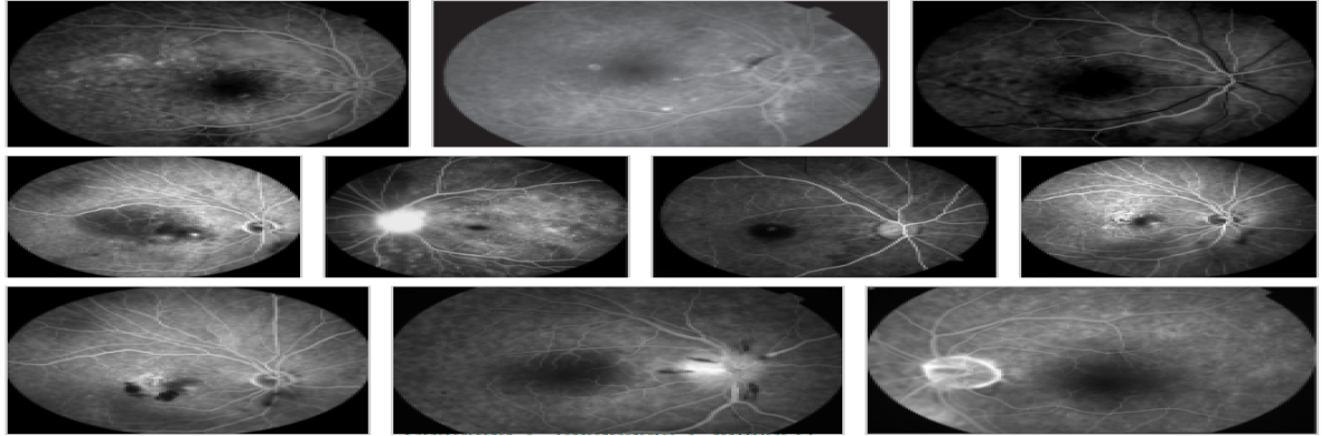
(b)

Figure 7: Comparison of the nearest images retrieved from the existing OpenI system (a) and our proposed system (b). The first image in each of the subfigures is the query image, and the remaining are the nearest images in the decreasing order of their similarity to the query image.

5.3 Effect of Medical Image Features and DenseLinkSearch on Open-i Service

Open-i service at the National Library of Medicine enables search and retrieval of abstracts and images from the open source literature and biomedical image collections. We aim to improve the Open-i image search service by the proposed medical feature extraction, and DenseLinkSearch approaches. We have shown the effect of the proposed approaches for retrieving similar images in Fig. 7. It is clearly illustrated that the proposed medical features extraction with the effective DenseLinkSearch is able to retrieve similar retinal images given an image of retina as query, while the current Open system retrieves mostly brain images as the nearest images to the same retinal image.

6 Conclusion

In this paper, we introduced an effective approach to nearest neighbor search that focuses on traversing the links created during indexing to reduce the distance computation for NNS. We evaluated multiple state-of-the-art approximate NNS algorithms and tree-based algorithms on multiple benchmark datasets in a comprehensive manner. The proposed DenseLinkSearch outperformed the existing approaches, where our approach achieves $\geq 99\%$ R@10 with the lowest average time/query on most of the benchmark datasets. In addition, we explored the role of image feature extractors for medical image retrieval tasks. We experimented with multiple pre-trained vision models and devised an effective approach for image feature extractors that outperformed the pre-trained vision model-based image feature extractors with a fair margin on multiple evaluation metrics.

Appendix A Hyper-parameters Details

	Artificial	Faces	Corel	MNIST	FMNIST	CovType
Ball Tree	leaf_size=9K	leaf_size=4500	leaf_size=58K	leaf_size=60K	leaf_size=45K	leaf_size=580K
KD Tree	leaf_size=9K	leaf_size=6K	leaf_size=58K	leaf_size=30K	leaf_size=45K	leaf_size=580K
RP Forest	leaf_size=900 n_trees=10	leaf_size=600 n_trees=15	leaf_size=3800 n_trees=15	leaf_size=6K n_trees=10	leaf_size=4K n_trees=15	leaf_size=29K n_trees=20
FAISS-LSH	n_bits=16384	n_bits=16384	n_bits=4096	n_bits=4096	n_bits=4096	n_bits=4096
FAISS-IVF	n_list=5	n_list=5	n_list=5	n_list=5	n_list=5	n_list=5
FAISS-IVFPQfs	n_list=5	n_list=5	n_list=10	n_list=5	n_list=5	n_list=100
Annoy	n_trees=500	n_trees=500	n_trees=500	n_trees=500	n_trees=500	n_trees=300
MRPT	-	-	-	-	-	-
HNSW	ef_construction=100 M=50	ef_construction=100 M=10	ef_construction=100 M=50	ef_construction=100 M=50	ef_construction=100 M=100	ef_construction=100 M=20
ScaNN	n_leaves=1 avq_threshold=0.20 dims_per_block=2	n_leaves=1 avq_threshold=0.20 dims_per_block=2	n_leaves=1 avq_threshold=0.20 dims_per_block=2	n_leaves=1 avq_threshold=0.2 dims_per_block=2	n_leaves=1 avq_threshold=0.2 dims_per_block=2	n_leaves=5000 avq_threshold=0.2 dims_per_block=2
DLS	$K_{index}$=50 $K_{search}$=20	$K_{index}$=50 $K_{search}$=20	$K_{index}$=50 $K_{search}$=10	$K_{index}$=40 $K_{search}$=15	$K_{index}$=50 $K_{search}$=10	$K_{index}$=40 $K_{search}$=50

Table 7: The hyper-parameters details that resulted in the best performance of the NNS approaches on benchmark datasets.

	TinyImages	Twitter	YearPred	SIFT	GIST	OpenI-ResNet	OpenI-ConvNeXt
Ball Tree	leaf_size=60K	leaf_size=570K	leaf_size=500K	leaf_size=700K	leaf_size=700K	NA	NA
KD Tree	leaf_size=60K	leaf_size=570K	leaf_size=500K	leaf_size=500K	leaf_size=500K	NA	NA
RP Forest	leaf_size=6K n_trees=15	leaf_size=57K n_trees=10	leaf_size=30K n_trees=15	leaf_size=5K n_trees=200	leaf_size=5K n_trees=200	NA	NA
FAISS-LSH	n_bits=4096	n_bits=4096	n_bits=4096	n_bits=4096	n_bits=4096	n_bits=4096	n_bits=4096
FAISS-IVF	n_list=5	n_list=5	n_list=5	n_list=5	n_list=5	n_list=5	n_list=25
FAISS-IVFPQfs	n_list=5	n_list=100	n_list=5	n_list=5	n_list=5	n_list=5	n_list=5
Annoy	n_trees=1000	n_trees=500	n_trees=500	n_trees=500	n_trees=1000	n_trees=1000	n_trees=500
MRPT	-	-	-	-	-	-	-
HNSW	ef_construction=100 M=100	ef_construction=100 M=50	ef_construction=100 M=50	ef_construction=100 M=200	ef_construction=100 M=200	ef_construction=100 M=100	ef_construction=100 M=100
ScaNN	n_leaves=1 avq_threshold=0.2 dims_per_block=2	n_leaves=75 avq_threshold=0.2 dims_per_block=2	n_leaves=1 avq_threshold=0.2 dims_per_block=2	n_leaves=1 avq_threshold=0.2 dims_per_block=2	n_leaves=1 avq_threshold=0.2 dims_per_block=2	n_leaves=1 avq_threshold=0.2 dims_per_block=2	n_leaves=1 avq_threshold=0.2 dims_per_block=2
DLS	$K_{index}$=20 $K_{search}$=50	$K_{index}$=30 $K_{search}$=20	$K_{index}$=30 $K_{search}$=25	$K_{index}$=40 $K_{search}$=30	$K_{index}$=40 $K_{search}$=55	$K_{index}$=110 $K_{search}$=35	$K_{index}$=30 $K_{search}$=110

Table 8: The hyper-parameters details that resulted in the best performance of the NNS approaches on benchmark datasets.

Appendix B Additional Results

	FAISS-LSH		FAISS-IVF		FAISS-IVFPQfs
	ATPQ (ms) $\downarrow$	R@10 (%) $\uparrow$	ATPQ (ms) $\downarrow$	R@10 (%) $\uparrow$	ATPQ (ms) $\downarrow$	R@10 (%) $\uparrow$
Artificial	3.754	49.63	0.061	39.86	0.030	30.11
Faces	3.772	47.56	0.044	89.46	0.027	42.27
Corel	6.699	66.23	0.217	90.50	0.0260	31.22
MNIST	7.396	68.16	4.683	86.02	0.292	79.29
FMNIST	7.921	43.86	4.986	92.99	0.314	81.12
CovType	64.746	65.35	6.532	99.22	0.036	2.528
TinyImages	10.501	27.62	3.074	73.11	0.217	50.76
Twitter	65.131	17.62	10.192	97.23	0.042	00.78
YearPred	58.845	22.97	7.299	90.48	0.241	8.731
SIFT	115.584	73.38	13.410	89.00	1.020	57.02
GIST	118.554	25.42	140.993	78.59	10.896	52.84
OpenI-ResNet	1684.21	56.26	869.72	85.80	56.07	58.37
OpenI-ConvNeXt	1379.24	61.48	2475.75	90.20	171.90	75.01

Table 9: Performance comparison of the FAISS implementation of multiple NNS approaches on benchmark datasets. The highlighted cells represent the approach having maximum R@10 amongst all the approaches.

Appendix C Pseudo codes of the Indexing and DenseLinkSearch

See pages - of figures/pseudocodes/Open_i_Search_Algorithm_v2.pdf

References

- Almalawi et al. [2015] Almalawi, A. M., Fahad, A., Tari, Z., Cheema, M. A., & Khalil, I. (2015). nnvwc: An efficient -nearest neighbors approach based on various-widths clustering. IEEE Transactions on Knowledge and Data Engineering, 28, 68–81.
- Antani et al. [2004] Antani, S., Long, L. R., & Thoma, G. R. (2004). Content-based image retrieval for large biomedical image archives. In MEDINFO 2004 (pp. 829–833). IOS Press.
- Antani et al. [2007] Antani, S. K., Deserno, T. M., Long, L. R., Güld, M. O., Neve, L., & Thoma, G. R. (2007). Interfacing global and local cbir systems for medical image retrieval. In Bildverarbeitung für die Medizin 2007 (pp. 166–171). Springer.
- Ba et al. [2016] Ba, J. L., Kiros, J. R., & Hinton, G. E. (2016). Layer normalization. arXiv preprint arXiv:1607.06450, .
- Babenko & Lempitsky [2014] Babenko, A., & Lempitsky, V. (2014). The inverted multi-index. IEEE transactions on pattern analysis and machine intelligence, 37, 1247–1260.
- Babenko et al. [2014] Babenko, A., Slesarev, A., Chigorin, A., & Lempitsky, V. (2014). Neural codes for image retrieval. In European conference on computer vision (pp. 584–599). Springer.
- [7] Bernhardsson, E. (). URL: https://github.com/spotify/annoy.
- Beygelzimer et al. [2006] Beygelzimer, A., Kakade, S., & Langford, J. (2006). Cover trees for nearest neighbor. In Proceedings of the 23rd international conference on Machine learning (pp. 97–104).
- Blackard & Dean [1999] Blackard, J. A., & Dean, D. J. (1999). Comparative accuracies of artificial neural networks and discriminant analysis in predicting forest cover types from cartographic variables. Computers and electronics in agriculture, 24, 131–151.
- Botta et al. [1993] Botta, M., Giordana, A., & Saitta, L. (1993). Learning fuzzy concept definitions. In [Proceedings 1993] Second IEEE International Conference on Fuzzy Systems (pp. 18–22). IEEE.
- Boytsov & Naidan [2013] Boytsov, L., & Naidan, B. (2013). Learning to prune in metric and non-metric spaces. Advances in Neural Information Processing Systems, 26.
- Bressan et al. [2019] Bressan, R. S., Bugatti, P. H., & Saito, P. T. (2019). Breast cancer diagnosis through active learning in content-based image retrieval. Neurocomputing, 357, 1–10.
- Buckley & Voorhees [2004] Buckley, C., & Voorhees, E. M. (2004). Retrieval evaluation with incomplete information. In Proceedings of the 27th annual international ACM SIGIR conference on Research and development in information retrieval (pp. 25–32).
- Cao et al. [2020] Cao, B., Araujo, A., & Sim, J. (2020). Unifying deep local and global features for image search. In European Conference on Computer Vision (pp. 726–743). Springer.
- Cao et al. [2014] Cao, Y., Steffey, S., He, J., Xiao, D., Tao, C., Chen, P., & Müller, H. (2014). Medical image retrieval: a multimodal approach. Cancer informatics, 13, CIN–S14053.
- Chen et al. [2021] Chen, W., Liu, Y., Wang, W., Bakker, E. M., Georgiou, T., Fieguth, P., Liu, L., & Lew, M. (2021). Deep image retrieval: A survey. ArXiv, .
- Ciaccia et al. [1997] Ciaccia, P., Patella, M., & Zezula, P. (1997). M-tree: An efficient access method for similarity search in metric spaces. In Vldb (pp. 426–435). volume 97.
- Clough et al. [2004] Clough, P., Sanderson, M., & Müller, H. (2004). The clef cross language image retrieval track (imageclef) 2004. In International Conference on Image and Video Retrieval (pp. 243–251). Springer.
- Conjeti et al. [2016] Conjeti, S., Mesbah, S., Negahdar, M., Rautenberg, P. L., Zhang, S., Navab, N., & Katouzian, A. (2016). Neuron-miner: an advanced tool for morphological search and retrieval in neuroscientific image databases. Neuroinformatics, 14, 369–385.
- Cortes & Vapnik [1995] Cortes, C., & Vapnik, V. (1995). Support-vector networks. Machine learning, 20, 273–297.
- Dasgupta & Freund [2008] Dasgupta, S., & Freund, Y. (2008). Random projection trees and low dimensional manifolds. In Proceedings of the fortieth annual ACM symposium on Theory of computing (pp. 537–546).
- Datar et al. [2004] Datar, M., Immorlica, N., Indyk, P., & Mirrokni, V. S. (2004). Locality-sensitive hashing scheme based on p-stable distributions. In Proceedings of the twentieth annual symposium on Computational geometry (pp. 253–262).
- Demner-Fushman et al. [2012] Demner-Fushman, D., Antani, S., Simpson, M., & Thoma, G. R. (2012). Design and development of a multimodal biomedical information retrieval system. Journal of Computing Science and Engineering, 6, 168–177.
- Depeursinge et al. [2011] Depeursinge, A., Zrimec, T., Busayarat, S., & Müller, H. (2011). 3d lung image retrieval using localized features. In Medical Imaging 2011: Computer-Aided Diagnosis (p. 79632E). International Society for Optics and Photonics volume 7963.
- Do & Cheung [2017] Do, T.-T., & Cheung, N.-M. (2017). Embedding based on function approximation for large scale image search. IEEE transactions on pattern analysis and machine intelligence, 40, 626–638.
- Dollár et al. [2009] Dollár, P., Tu, Z., Perona, P., & Belongie, S. (2009). Integral channel features, .
- Dosovitskiy et al. [2020] Dosovitskiy, A., Beyer, L., Kolesnikov, A., Weissenborn, D., Zhai, X., Unterthiner, T., Dehghani, M., Minderer, M., Heigold, G., Gelly, S. et al. (2020). An image is worth 16x16 words: Transformers for image recognition at scale. In International Conference on Learning Representations.
- Dua & Graff [2017] Dua, D., & Graff, C. (2017). UCI machine learning repository. URL: http://archive.ics.uci.edu/ml.
- Friedman et al. [1977] Friedman, J. H., Bentley, J. L., & Finkel, R. A. (1977). An algorithm for finding best matches in logarithmic expected time. ACM Transactions on Mathematical Software (TOMS), 3, 209–226.
- Fukunaga & Narendra [1975] Fukunaga, K., & Narendra, P. M. (1975). A branch and bound algorithm for computing k-nearest neighbors. IEEE transactions on computers, 100, 750–753.
- Gong et al. [2014] Gong, Y., Wang, L., Guo, R., & Lazebnik, S. (2014). Multi-scale orderless pooling of deep convolutional activation features. In European conference on computer vision (pp. 392–407). Springer.
- Guo et al. [2020] Guo, R., Sun, P., Lindgren, E., Geng, Q., Simcha, D., Chern, F., & Kumar, S. (2020). Accelerating large-scale inference with anisotropic vector quantization. In International Conference on Machine Learning (pp. 3887–3896). PMLR.
- Gupta et al. [2022] Gupta, D., Attal, K., & Demner-Fushman, D. (2022). A dataset for medical instructional video classification and question answering. arXiv preprint arXiv:2201.12888, .
- Gupta & Demner-Fushman [2022] Gupta, D., & Demner-Fushman, D. (2022). Overview of the MedVidQA 2022 shared task on medical video question-answering. In Proceedings of the 21st Workshop on Biomedical Language Processing (pp. 264–274). Dublin, Ireland: Association for Computational Linguistics. URL: https://aclanthology.org/2022.bionlp-1.25. doi:10.18653/v1/2022.bionlp-1.25.
- Gupta et al. [2021] Gupta, D., Suman, S., & Ekbal, A. (2021). Hierarchical deep multi-modal network for medical visual question answering. Expert Systems with Applications, 164, 113993.
- Haralick [1979] Haralick, R. M. (1979). Statistical and structural approaches to texture. Proceedings of the IEEE, 67, 786–804.
- He et al. [2016] He, K., Zhang, X., Ren, S., & Sun, J. (2016). Deep residual learning for image recognition. In Proceedings of the IEEE conference on computer vision and pattern recognition (pp. 770–778).
- Hendrycks & Gimpel [2016] Hendrycks, D., & Gimpel, K. (2016). Gaussian error linear units (gelus). arXiv preprint arXiv:1606.08415, .
- Hochreiter [1998] Hochreiter, S. (1998). The vanishing gradient problem during learning recurrent neural nets and problem solutions. International Journal of Uncertainty, Fuzziness and Knowledge-Based Systems, 6, 107–116.
- Hsu et al. [2007] Hsu, W., Long, L. R., Antani, S. et al. (2007). Spirs: a framework for content-based image retrieval from large biomedical databases. MedInfo, 12, 188–192.
- Huang et al. [2017] Huang, G., Liu, Z., Van Der Maaten, L., & Weinberger, K. Q. (2017). Densely connected convolutional networks. In Proceedings of the IEEE conference on computer vision and pattern recognition (pp. 4700–4708).
- Hwang et al. [2018] Hwang, Y., Baek, M., Kim, S., Han, B., & Ahn, H.-K. (2018). Product quantized translation for fast nearest neighbor search. In Proceedings of the AAAI Conference on Artificial Intelligence. volume 32.
- Hwang et al. [2012] Hwang, Y., Han, B., & Ahn, H.-K. (2012). A fast nearest neighbor search algorithm by nonlinear embedding. In 2012 IEEE Conference on Computer Vision and Pattern Recognition (pp. 3053–3060). IEEE.
- Hyvönen et al. [2016] Hyvönen, V., Pitkänen, T., Tasoulis, S., Jääsaari, E., Tuomainen, R., Wang, L., Corander, J., & Roos, T. (2016). Fast nearest neighbor search through sparse random projections and voting. In Big Data (Big Data), 2016 IEEE International Conference on (pp. 881–888). IEEE.
- Jegou et al. [2010] Jegou, H., Douze, M., & Schmid, C. (2010). Product quantization for nearest neighbor search. IEEE transactions on pattern analysis and machine intelligence, 33, 117–128.
- Jeong et al. [2006] Jeong, S., Kim, S.-W., Kim, K., & Choi, B.-U. (2006). An effective method for approximating the euclidean distance in high-dimensional space. In International Conference on Database and Expert Systems Applications (pp. 863–872). Springer.
- Johnson et al. [2019] Johnson, J., Douze, M., & Jégou, H. (2019). Billion-scale similarity search with GPUs. IEEE Transactions on Big Data, 7, 535–547.
- Kalpathy-Cramer et al. [2015] Kalpathy-Cramer, J., de Herrera, A. G. S., Demner-Fushman, D., Antani, S., Bedrick, S., & Müller, H. (2015). Evaluating performance of biomedical image retrieval systems—an overview of the medical image retrieval task at imageclef 2004–2013. Computerized Medical Imaging and Graphics, 39, 55–61.
- Kalpathy-Cramer et al. [2011] Kalpathy-Cramer, J., Müller, H., Bedrick, S., Eggel, I., de Herrera, A. G. S., & Tsikrika, T. (2011). Overview of the clef 2011 medical image classification and retrieval tasks. In CLEF (notebook papers/labs/workshop) (pp. 97–112).
- Kamel & Faloutsos [1993] Kamel, I., & Faloutsos, C. (1993). Hilbert R-tree: An improved R-tree using fractals. Technical Report.
- Kassim et al. [2020] Kassim, Y. M., Palaniappan, K., Yang, F., Poostchi, M., Palaniappan, N., Maude, R. J., Antani, S., & Jaeger, S. (2020). Clustering-based dual deep learning architecture for detecting red blood cells in malaria diagnostic smears. IEEE Journal of Biomedical and Health Informatics, 25, 1735–1746.
- Khan et al. [2011] Khan, M. I., Acharya, B., Singh, B. K., & Soni, J. (2011). Content based image retrieval approaches for detection of malarial parasite in blood images. International Journal of Biometrics and Bioinformatics (IJBB), 5, 97.
- Lambin et al. [2012] Lambin, P., Rios-Velazquez, E., Leijenaar, R., Carvalho, S., Van Stiphout, R. G., Granton, P., Zegers, C. M., Gillies, R., Boellard, R., Dekker, A. et al. (2012). Radiomics: extracting more information from medical images using advanced feature analysis. European journal of cancer, 48, 441–446.
- LeCun et al. [1998] LeCun, Y., Bottou, L., Bengio, Y., & Haffner, P. (1998). Gradient-based learning applied to document recognition. Proceedings of the IEEE, 86, 2278–2324.
- Lehmann et al. [2004] Lehmann, T. M., Güld, M. O., Thies, C., Fischer, B., Spitzer, K., Keysers, D., Ney, H., Kohnen, M., Schubert, H., & Wein, B. B. (2004). Content-based image retrieval in medical applications. Methods of information in medicine, 43, 354–361.
- Li et al. [2018a] Li, M., Zhang, Y., Sun, Y., Wang, W., Tsang, I. W., & Lin, X. (2018a). An efficient exact nearest neighbor search by compounded embedding. In International Conference on Database Systems for Advanced Applications (pp. 37–54). Springer.
- Li et al. [2018b] Li, Z., Zhang, X., Müller, H., & Zhang, S. (2018b). Large-scale retrieval for medical image analytics: A comprehensive review. Medical image analysis, 43, 66–84.
- Liu et al. [2018] Liu, Y., Wei, H., & Cheng, H. (2018). Exploiting lower bounds to accelerate approximate nearest neighbor search on high-dimensional data. Information Sciences, 465, 484–504.
- Liu et al. [2021] Liu, Z., Lin, Y., Cao, Y., Hu, H., Wei, Y., Zhang, Z., Lin, S., & Guo, B. (2021). Swin transformer: Hierarchical vision transformer using shifted windows. In Proceedings of the IEEE/CVF International Conference on Computer Vision (pp. 10012–10022).
- Liu et al. [2022] Liu, Z., Mao, H., Wu, C.-Y., Feichtenhofer, C., Darrell, T., & Xie, S. (2022). A convnet for the 2020s. In Proceedings of the IEEE/CVF Conference on Computer Vision and Pattern Recognition (pp. 11976–11986).
- Lou et al. [2018] Lou, Y., Bai, Y., Wang, S., & Duan, L.-Y. (2018). Multi-scale context attention network for image retrieval. In Proceedings of the 26th ACM international conference on Multimedia (pp. 1128–1136).
- Malkov et al. [2014] Malkov, Y., Ponomarenko, A., Logvinov, A., & Krylov, V. (2014). Approximate nearest neighbor algorithm based on navigable small world graphs. Information Systems, 45, 61–68.
- Malkov & Yashunin [2018] Malkov, Y. A., & Yashunin, D. A. (2018). Efficient and robust approximate nearest neighbor search using hierarchical navigable small world graphs. IEEE transactions on pattern analysis and machine intelligence, 42, 824–836.
- McDonald et al. [2015] McDonald, R. J., Schwartz, K. M., Eckel, L. J., Diehn, F. E., Hunt, C. H., Bartholmai, B. J., Erickson, B. J., & Kallmes, D. F. (2015). The effects of changes in utilization and technological advancements of cross-sectional imaging on radiologist workload. Academic radiology, 22, 1191–1198.
- Mesbah et al. [2015] Mesbah, S., Conjeti, S., Kumaraswamy, A., Rautenberg, P., Navab, N., & Katouzian, A. (2015). Hashing forests for morphological search and retrieval in neuroscientific image databases. In International Conference on Medical Image Computing and Computer-Assisted Intervention (pp. 135–143). Springer.
- Müller et al. [2012] Müller, H., de Herrera, A. G. S., Kalpathy-Cramer, J., Demner-Fushman, D., Antani, S. K., & Eggel, I. (2012). Overview of the imageclef 2012 medical image retrieval and classification tasks. In CLEF (online working notes/labs/workshop) (pp. 1–16).
- Müller et al. [2009] Müller, H., Kalpathy-Cramer, J., Eggel, I., Bedrick, S., Radhouani, S., Bakke, B., Kahn, C. E., & Hersh, W. (2009). Overview of the clef 2009 medical image retrieval track. In Workshop of the Cross-Language Evaluation Forum for European Languages (pp. 72–84). Springer.
- Nazari & Fatemizadeh [2010] Nazari, M. R., & Fatemizadeh, E. (2010). A cbir system for human brain magnetic resonance image indexing. International Journal of Computer Applications, 7, 33–37.
- Omohundro [1989] Omohundro, S. M. (1989). Five balltree construction algorithms. International Computer Science Institute Berkeley.
- Ortega et al. [1998] Ortega, M., Rui, Y., Chakrabarti, K., Porkaew, K., Mehrotra, S., & Huang, T. S. (1998). Supporting ranked boolean similarity queries in mars. IEEE Transactions on Knowledge and Data Engineering, 10, 905–925.
- Pedregosa et al. [2011] Pedregosa, F., Varoquaux, G., Gramfort, A., Michel, V., Thirion, B., Grisel, O., Blondel, M., Prettenhofer, P., Weiss, R., Dubourg, V., Vanderplas, J., Passos, A., Cournapeau, D., Brucher, M., Perrot, M., & Duchesnay, E. (2011). Scikit-learn: Machine learning in Python. Journal of Machine Learning Research, 12, 2825–2830.
- Pestov [2012] Pestov, V. (2012). Indexability, concentration, and vc theory. Journal of Discrete Algorithms, 13, 2–18.
- Prerau & Eskin [2000] Prerau, M. J., & Eskin, E. (2000). Unsupervised anomaly detection using an optimized k-nearest neighbors algorithm. Undergraduate Thesis, Columbia University: December, .
- Qayyum et al. [2017] Qayyum, A., Anwar, S. M., Awais, M., & Majid, M. (2017). Medical image retrieval using deep convolutional neural network. Neurocomputing, 266, 8–20.
- Radenović et al. [2018] Radenović, F., Tolias, G., & Chum, O. (2018). Fine-tuning cnn image retrieval with no human annotation. IEEE transactions on pattern analysis and machine intelligence, 41, 1655–1668.
- Rahman et al. [2011] Rahman, M. M., Antani, S. K., & Thoma, G. R. (2011). A learning-based similarity fusion and filtering approach for biomedical image retrieval using svm classification and relevance feedback. IEEE Transactions on Information Technology in Biomedicine, 15, 640–646.
- Rahman et al. [2008] Rahman, M. M., Desai, B. C., & Bhattacharya, P. (2008). Medical image retrieval with probabilistic multi-class support vector machine classifiers and adaptive similarity fusion. Computerized Medical Imaging and Graphics, 32, 95–108.
- Rahman et al. [2013] Rahman, M. M., You, D., Simpson, M. S., Antani, S. K., Demner-Fushman, D., & Thoma, G. R. (2013). Multimodal biomedical image retrieval using hierarchical classification and modality fusion. International Journal of Multimedia Information Retrieval, 2, 159–173.
- Rajaraman et al. [2018] Rajaraman, S., Antani, S. K., Poostchi, M., Silamut, K., Hossain, M. A., Maude, R. J., Jaeger, S., & Thoma, G. R. (2018). Pre-trained convolutional neural networks as feature extractors toward improved malaria parasite detection in thin blood smear images. PeerJ, 6, e4568.
- Razavian et al. [2016] Razavian, A. S., Sullivan, J., Carlsson, S., & Maki, A. (2016). Visual instance retrieval with deep convolutional networks. ITE Transactions on Media Technology and Applications, 4, 251–258.
- Ridnik et al. [2021] Ridnik, T., Ben-Baruch, E., Noy, A., & Zelnik-Manor, L. (2021). Imagenet-21k pretraining for the masses. In Thirty-fifth Conference on Neural Information Processing Systems Datasets and Benchmarks Track (Round 1).
- Russakovsky et al. [2015] Russakovsky, O., Deng, J., Su, H., Krause, J., Satheesh, S., Ma, S., Huang, Z., Karpathy, A., Khosla, A., Bernstein, M., Berg, A. C., & Fei-Fei, L. (2015). ImageNet Large Scale Visual Recognition Challenge. International Journal of Computer Vision (IJCV), 115, 211–252. doi:10.1007/s11263-015-0816-y.
- Santurkar et al. [2018] Santurkar, S., Tsipras, D., Ilyas, A., & Madry, A. (2018). How does batch normalization help optimization? Advances in neural information processing systems, 31.
- Sharif Razavian et al. [2014] Sharif Razavian, A., Azizpour, H., Sullivan, J., & Carlsson, S. (2014). Cnn features off-the-shelf: an astounding baseline for recognition. In Proceedings of the IEEE conference on computer vision and pattern recognition workshops (pp. 806–813).
- Simonyan & Zisserman [2014] Simonyan, K., & Zisserman, A. (2014). Very deep convolutional networks for large-scale image recognition. arXiv preprint arXiv:1409.1556, .
- Sproull [1991] Sproull, R. F. (1991). Refinements to nearest-neighbor searching ink-dimensional trees. Algorithmica, 6, 579–589.
- Szegedy et al. [2015] Szegedy, C., Liu, W., Jia, Y., Sermanet, P., Reed, S., Anguelov, D., Erhan, D., Vanhoucke, V., & Rabinovich, A. (2015). Going deeper with convolutions. In Proceedings of the IEEE conference on computer vision and pattern recognition (pp. 1–9).
- Szegedy et al. [2016] Szegedy, C., Vanhoucke, V., Ioffe, S., Shlens, J., & Wojna, Z. (2016). Rethinking the inception architecture for computer vision. In Proceedings of the IEEE conference on computer vision and pattern recognition (pp. 2818–2826).
- Vaswani et al. [2017] Vaswani, A., Shazeer, N., Parmar, N., Uszkoreit, J., Jones, L., Gomez, A. N., Kaiser, Ł., & Polosukhin, I. (2017). Attention is all you need. Advances in neural information processing systems, 30.
- Wang [2011] Wang, X. (2011). A fast exact k-nearest neighbors algorithm for high dimensional search using k-means clustering and triangle inequality. In The 2011 International Joint Conference on Neural Networks (pp. 1293–1299). IEEE.
- Wei et al. [2009] Wei, L., Yang, Y., & Nishikawa, R. M. (2009). Microcalcification classification assisted by content-based image retrieval for breast cancer diagnosis. Pattern recognition, 42, 1126–1132.
- Wightman [2019] Wightman, R. (2019). Pytorch image models. https://github.com/rwightman/pytorch-image-models. doi:10.5281/zenodo.4414861.
- Xiao et al. [2017] Xiao, H., Rasul, K., & Vollgraf, R. (2017). Fashion-mnist: a novel image dataset for benchmarking machine learning algorithms. arXiv preprint arXiv:1708.07747, .
- Xie et al. [2017] Xie, S., Girshick, R., Dollár, P., Tu, Z., & He, K. (2017). Aggregated residual transformations for deep neural networks. In Proceedings of the IEEE conference on computer vision and pattern recognition (pp. 1492–1500).
- Xue et al. [2008] Xue, Z., Long, L. R., Antani, S., Jeronimo, J., & Thoma, G. R. (2008). A web-accessible content-based cervicographic image retrieval system. In Medical Imaging 2008: PACS and Imaging Informatics (pp. 46–54). SPIE volume 6919.
- Yan et al. [2019] Yan, D., Wang, Y., Wang, J., Wang, H., & Li, Z. (2019). K-nearest neighbor search by random projection forests. IEEE Transactions on Big Data, 7, 147–157.
- Yianilos [1993] Yianilos, P. N. (1993). Data structures and algorithms for nearest neighbor. In Proceedings of the fourth annual ACM-SIAM Symposium on Discrete algorithms (p. 311). SIAM volume 66.
- Yu et al. [2020] Yu, J., Zhu, Z., Wang, Y., Zhang, W., Hu, Y., & Tan, J. (2020). Cross-modal knowledge reasoning for knowledge-based visual question answering. Pattern Recognition, 108, 107563.
- Yu et al. [2017] Yu, W., Yang, K., Yao, H., Sun, X., & Xu, P. (2017). Exploiting the complementary strengths of multi-layer cnn features for image retrieval. Neurocomputing, 237, 235–241.
- Yue-Hei Ng et al. [2015] Yue-Hei Ng, J., Yang, F., & Davis, L. S. (2015). Exploiting local features from deep networks for image retrieval. In Proceedings of the IEEE conference on computer vision and pattern recognition workshops (pp. 53–61).
- Zhang et al. [2022] Zhang, H., Dong, Y., & Xu, D. (2022). Accelerating exact nearest neighbor search in high dimensional euclidean space via block vectors. International Journal of Intelligent Systems, 37, 1697–1722.
- Zhang et al. [2019] Zhang, Z., Xie, Y., Zhang, W., & Tian, Q. (2019). Effective image retrieval via multilinear multi-index fusion. IEEE Transactions on Multimedia, 21, 2878–2890.
- Zhong et al. [2021] Zhong, A., Li, X., Wu, D., Ren, H., Kim, K., Kim, Y., Buch, V., Neumark, N., Bizzo, B., Tak, W. Y. et al. (2021). Deep metric learning-based image retrieval system for chest radiograph and its clinical applications in covid-19. Medical Image Analysis, 70, 101993.