Temporally Consistent Transformers for Video Generation

Abstract

To generate accurate videos, algorithms have to understand the spatial and temporal dependencies in the world. Current algorithms enable accurate predictions over short horizons but tend to suffer from temporal inconsistencies. When generated content goes out of view and is later revisited, the model invents different content instead. Despite this severe limitation, no established benchmarks on complex data exist for rigorously evaluating video generation with long temporal dependencies. In this paper, we curate 3 challenging video datasets with long-range dependencies by rendering walks through 3D scenes of procedural mazes, Minecraft worlds, and indoor scans. We perform a comprehensive evaluation of current models and observe their limitations in temporal consistency. Moreover, we introduce the Temporally Consistent Transformer (TECO), a generative model that substantially improves long-term consistency while also reducing sampling time. By compressing its input sequence into fewer embeddings, applying a temporal transformer, and expanding back using a spatial MaskGit, TECO outperforms existing models across many metrics. Videos are available on the website: https://wilson1yan.github.io/teco

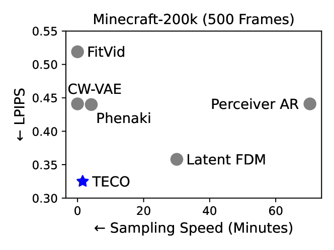
Figure 1: TECO generates temporally consistent videos of high fidelity (low LPIPS) over hundreds of frames while offering orders of magnitude faster sampling speed compared to previous video generation models.

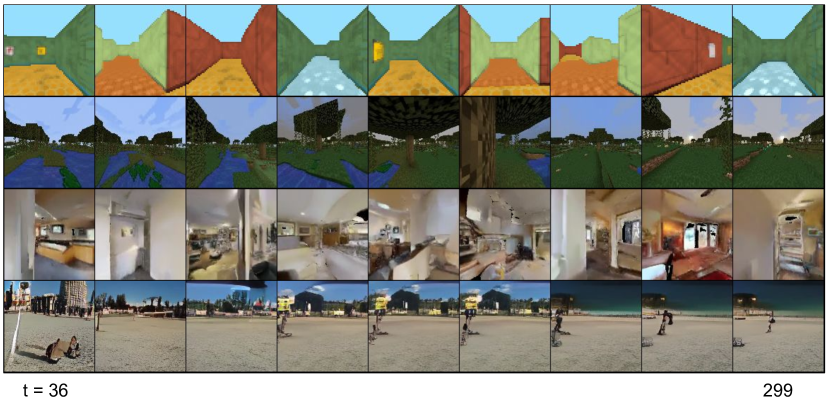
Figure 2: TECO generates sharp and consistent video predictions for hundreds of frames on challenging datasets. The figure shows evenly spaced frames of the 264 frame predictions, after being conditioned on 36 context frames. From top to bottom, the datasets are are DMLab, Minecraft, Habitat, and Kinetics-600.

1 Introduction

Recent work in video generation has seen tremendous progress (Ho et al., 2022; Clark et al., 2019; Yan et al., 2021; Le Moing et al., 2021; Ge et al., 2022; Tian et al., 2021; Luc et al., 2020) in producing high-fidelity and diverse samples on complex video data, which can largely be attributed to a combination of increased computational resources and more compute efficient high-capacity neural architectures. However, much of this progress has focused on generating short videos, where models perform well by basing their predictions on only a handful of previous frames.

Video prediction models with short context windows can generate long videos in a sliding window fashion. While the resulting videos can look impressive at first sight, they lack temporal consistency. We would like models to predict temporally consistent videos — where the same content is generated if a camera pans back to a previously observed location. On the other hand, the model should imagine a new part of the scene for locations that have not yet been observed, and future predictions should remain consistent to this newly imagined part of the scene.

Prior work has investigated techniques for modeling long-term dependencies, such as temporal hierarchies (Saxena et al., 2021) and strided sampling with frame-wise interpolation (Ge et al., 2022; Hong et al., 2022). Other methods train on sparse sets of frames selected out of long videos (Harvey et al., 2022; Skorokhodov et al., 2021; Clark et al., 2019; Saito & Saito, 2018; Yu et al., 2022), or model videos via compressed representations (Yan et al., 2021; Rakhimov et al., 2020; Le Moing et al., 2021; Seo et al., 2022; Gupta et al., 2022; Walker et al., 2021). Refer to Appendix L for more detailed discussion on related work.

Despite this progress, many methods still have difficulty scaling to datasets with many long-range dependencies. While Clockwork-VAE (Saxena et al., 2021) trains on long sequences, it is limited by training time (due to recurrence) and difficult to scale to complex data. On the other hand, transformer-based methods over latent spaces (Yan et al., 2021) scale poorly to long videos due to quadratic complexity in attention, with long videos containing tens of thousands of tokens. Methods that train on subsets of tokens are limited by truncated backpropagation through time (Hutchins et al., 2022; Rae et al., 2019; Dai et al., 2019) or naive temporal operations (Hawthorne et al., 2022).

In addition, there generally do not exist benchmarks for properly evaluating temporal consistency in video generation methods, where prior works either focus on generating long videos where short-term dependencies are sufficient for accurate prediction (Ge et al., 2022; Skorokhodov et al., 2021) and/or rely on metrics such as FVD (Unterthiner et al., 2019) which are more sensitive to image fidelity rather than capture long-range temporal dependencies.

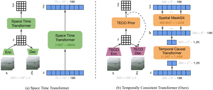
Figure 3: The architectural design of TECO. (a) Prior work on video generation models over VQ codes adopt a single spatio-temporal transformer over all codes. This is prohibitive when scaling to long sequences due to the quadratic complexity of attention. (b) We propose a novel and efficient architecture that aggressively downsamples in space before feeding into a temporal transformer, and then expands back out with a spatial MaskGit that is separately applied per frame. In the figure, the transformer blocks show the number of attention links. On training sequences of $300$ frames, TECO sees orders of magnitude more efficiency over existing models, allowing the use of larger models for a given compute budget.

In this paper, we introduce a set of novel long-horizon video generation benchmarks, as well as corresponding evaluation metrics to better capture temporal consistency. In addition, we propose Temporally Consistent Video Transformer (TECO), a vector-quantized latent dynamics model that effectively models long-term dependencies in a compact representation space using efficient transformers. The key contributions are summarized as follows:

• To better evaluate temporal consistency in video predictions, we propose 3 video datasets with long-range dependencies including metrics, generated from 3D scenes in DMLab (Beattie et al., 2016), Minecraft (Guss et al., 2019), and Habitat (Szot et al., 2021; Savva et al., 2019)

• We benchmark SOTA video generation models on the datasets and analyze capabilities of each in learning long-horizon dependencies.

• We introduce TECO, an efficient and scalable video generation model that learns compressed representations to allow for efficient training and generation. We show that TECO has strong performance on a variety of difficult video prediction tasks, and is able to leverage long-term temporal context to generate high quality videos with consistency while maintaining fast sampling speed.

2 Preliminaries

2.1 VQ-GAN

VQ-GAN (Esser et al., 2021; Van Den Oord et al., 2017) is an autoencoder that learns to compress data into discrete latents, consisting of an encoder $E$, decoder $G$, codebook $C$, and discriminator $D$. Given an image $x\in\mathbb{R}^{H\times W\times 3}$, the encoder $E$ maps $x$ to its latent representation $h\in\mathbb{R}^{H^{\prime}\times W^{\prime}\times D}$, which is quantized by nearest neighbors lookup in a codebook of embeddings $C=\{e_{i}\}^{K}_{i=1}$ to produce $z\in\mathbb{R}^{H^{\prime}\times W^{\prime}\times D}$. $z$ is fed through decoder $G$ to reconstruct $x$. A straight-through estimator (Bengio, 2013) is used to maintain gradient flow through the quantization step. The codebook optimizes the following loss:

$$\begin{aligned} \mathcal{L}_{\mathrm{VQ}}&=\left\lVert\,\operatorname{sg}(h)-e\,\right\rVert_{2}^{2}+\beta\left\lVert\,h-\operatorname{sg}(e)\,\right\rVert_{2}^{2}\end{aligned}$$ (1)

where $\beta=0.25$ is a hyperparameter, and $e$ is the nearest-neighbors embedding from $C$. For reconstruction, VQ-GAN replaces the original $\ell_{2}$ loss with a perceptual loss (Zhang et al., 2012), $\mathcal{L}_{\mathrm{LPIPS}}$. Finally, in order to encourage higher-fidelity samples, patch-level discriminator $D$ is trained to classify between real and reconstructed images, with:

$$\begin{aligned} \mathcal{L}_{\mathrm{GAN}}&=\log{D(x)}+\log(1-D(\hat{x}))\end{aligned}$$ (2)

Overall, VQ-GAN optimizes the following loss:

$$\begin{aligned} \min_{E,G,C}\max_{D}\,\,\,\mathcal{L}_{\mathrm{LPIPS}}+\mathcal{L}_{\mathrm{VQ}}+\lambda\mathcal{L}_{\mathrm{GAN}}\end{aligned}$$ (3)

where $\lambda=\frac{\left\lVert\,\nabla_{G_{L}}\mathcal{L}_{\mathrm{LPIPS}}\,\right\rVert_{2}}{\left\lVert\,\nabla_{G_{L}}\mathcal{L}_{\mathrm{GAN}}\,\right\rVert_{2}+\delta}$ is an adaptive weight, $G_{L}$ is the last decoder layer, $\delta=10^{-6}$, and $\mathcal{L}_{LPIPS}$ is the same distance metric described in Zhang et al. (2012).

2.2 MaskGit

MaskGit (Chang et al., 2022) models distributions over discrete tokens, such as produced by a VQ-GAN. It generates images with competitive sample quality to autoregressive models at a fraction of the sampling cost by using a masked token prediction objective during training. Formally, we denote $z\in\mathbb{Z}^{H\times W}$ as the discrete latent tokens representing an image. For each training step, we uniformly sample $t\in[0,1)$ and randomly generate a mask $m\in\{0,1\}^{H\times W}$ with $N=\lceil\gamma HW\rceil$ masked values, where $\gamma=\cos\left(\frac{\pi}{2}t\right)$. Then, MaskGit learns to predict the masked tokens with the following objective

$$\begin{aligned} \mathcal{L}_{\mathrm{mask}}=-\operatorname{E}_{z\in\mathcal{D}}\big{[}\log p(z\;|\;z\odotm)\big{]}.\end{aligned}$$ (4)

During inference, because MaskGit has been trained to model any set of unconditional and conditional probabilities, we can sample any subset of tokens per sampling iteration. (Chang et al., 2022) introduces a confidence-based sampling mechanism whereas other work (Lee et al., 2022) proposes an iterative sample-and-revise approach.

3 TECO

We present Temporally Consistent Video Transformer (TECO), a video generation model that more efficiently scales to training on longer horizon videos.

3.1 Architectural Overview

Our proposed framework is shown in Figure 3, where $x_{1:T}$ consists of a sequence of video frames. Our primary innovation centers around designing a more efficient architecture that can scale to long sequences. Prior SOTA methods (Yan et al., 2021; Ge et al., 2022; Villegas et al., 2022) over VQ-codes all train a single spatio-temporal transformer to model every code, however, this becomes prohibitively expensive with sequences containing tens of thousands of tokens. On the other hand, these models have shown to be able to learn highly multi-modal distributions and scale well on complex video. As such, we design the TECO architecture with the intention to retain its high-capacity scaling properties, while ensuring orders of magnitude more efficient training and inference. In the following sections, we motivate each component for our model, with several specific design choices to ensure efficiency and scalability. TECO consists of four components:

$$\begin{aligned} &\text{Encoder:}\quad&&z_{t}=E(x_{t},x_{t-1})\qquad\\ &\text{Temporal Transformer:}&&h_{t}=H(z_{\leq t})\\ &\text{Spatial MaskGit:}\quad&&p(z_{t}\mid h_{t-1})\\ &\text{Decoder:}&&p(x_{t}\mid z_{t},h_{t-1})\end{aligned}$$ (5)

Encoder We can achieve compressed representations by leveraging spatio-temporal redundancy in video data. To do this, we learn a CNN encoder $z_{t}=E(x_{t},x_{t-1})$ which encodes the current frame $x_{t}$ conditioned on the previous frame by channel-wise concatenating $x_{t-1}$, and then quantizes the output using codebook $C$ to produce $z_{t}$. We apply the VQ loss defined in Equation 1 per timestep. In addition, we $\ell_{2}$-normalize the codebook and embeddings to encourage higher codebook usage (Yu et al., 2021). The first frame is concatenated with zeros and does not quantize $z_{1}$ to prevent information loss.

Temporal Transformer Compressed, discrete latents are more lossy and tend to require higher spatial resolutions compared to continuous latents. Therefore, before modeling temporal information, we apply a single strided convolution to downsample each discrete latent $z_{t}$, where visually simpler datasets allow for more downsampling and visually complex datasets require less downsampling. Afterwards, we learn a large transformer to model temporal dependencies, and then apply a transposed convolution to upsample our representation back to the original resolution of $z_{t}$. In summary, we use the following architecture:

$$\begin{aligned} h_{t}&=H(z_{<t})=\text{ConvT}(\text{Transformer}(\text{Conv}(z_{<t})))\end{aligned}$$ (6)

Decoder The decoder is an upsampling CNN that reconstructs $\hat{x_{t}}=D(z_{t},h_{t})$, where $z_{t}$ can be interpreted as the posterior of timestep $t$, and $h_{t}$ the output of the temporal transformer which summarizes information from previous timesteps. $z_{t}$ and $h_{t}$ are concatenated channel-wise and into the decoder. Together with the encoder, the decoder optimizes the following cross entropy reconstruction loss

$$\begin{aligned} \mathcal{L}_{\mathrm{recon}}&=-\textstyle\frac{1}{T}\sum_{t=1}^{T}\log p(x_{t}\mid z_{t},h_{t}).\end{aligned}$$ (7)

which encourages $z_{t}$ features to encode relative information between frames since the temporal transformer output $h_{t}$ aggregates information over time, learning more compressed codes for efficient modeling over longer sequences.

Spatial MaskGit Lastly, we use a MaskGit (Chang et al., 2022) to model the prior, $p(z_{t}\mid h_{t})$. We show that using a MaskGit prior allows for not just faster but also higher quality sampling compared to an autoregressive prior. During every training iteration, we follow prior work to sample a random mask $m_{t}$ and optimize

$$\begin{aligned} \mathcal{L}_{\mathrm{prior}}=-\textstyle\frac{1}{T}\sum_{t=1}^{T}\log p(z_{t}\mid z_{t}\odot m_{t}).\end{aligned}$$ (8)

where $h_{t}$ is concatenated channel-wise with masked $z_{t}$ to predict the masked tokens. During generation, we follow Lee et al. (2022), where we initially generate each frame in chunks of 8 at a time and then go through 2 revise rounds of re-generating half the tokens each time.

Training Objective The final objective is the following:

$$\mathcal{L}_{\mathrm{TECO}} =\mathcal{L}_{\mathrm{VQ}}+\mathcal{L}_{\mathrm{recon}}+\mathcal{L}_{\mathrm{prior}}$$ (9)

3.2 DropLoss

We propose DropLoss, a simple trick to allow for more scalable and efficient training (Figure 4). Due to its architecture design, TECO can be separated into two components: (1) learning temporal representations, consisting of the encoder and the temporal transformer, and (2) predicting future frames, consisting of the dynamics prior and decoder. We can increase training efficiency by dropping out random timesteps that are not decoded and thus omitted from the reconstruction loss. For example, given a video of T frames, we compute $h_{t}$ for all $t\in\{1,\dots,T\}$, and then compute the losses $\mathcal{L}_{\mathrm{prior}}$ and $\mathcal{L}_{\mathrm{recon}}$ for only 10% of the indices. Because random indices are selected each iteration, the model still needs to learn to accurately predict all timesteps. This reduces training costs significantly because the decoder and dynamics prior require non-trivial computations. DropLoss is applicable to both a wide class of architectures and to tasks beyond video prediction.

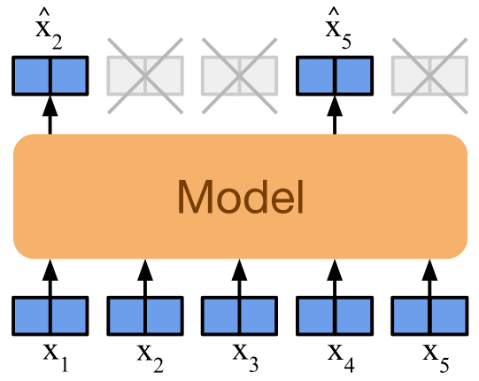
Figure 4: DropLoss improves training scalability on longer sequences by only computing the loss on a random subset of time indices for each training iteration. For TECO, we do not need to compute the decoder and MaskGit for dropped out timesteps.

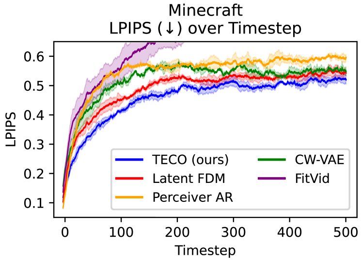
Figure 5: Quantitative comparisons between TECO and baseline methods in long-horizon temporal consistency, showing LPIPS between generated and ground-truth frames for each timestep. Timestep 0 corresponds to the first predicted frame (conditioning frames are not included in the plot). Our method is able to remain more temporally consistent over hundreds of timesteps of prediction compared to SOTA models.

4 Experiments

4.1 Datasets

We introduce three challenging video datasets to better measure long-range consistency in video prediction, centered around 3D environments in DMLab (Beattie et al., 2016), Minecraft (Guss et al., 2019), and Habitat (Savva et al., 2019), with videos of agents randomly traversing scenes of varying difficulty. These datasets require video prediction models to re-produce observed parts of scenes, and newly generate unobserved parts. In contrast, many existing video benchmarks do not have strong long-range dependencies, where a model with limited context is sufficient. Refer to Appendix M for further details on each dataset.

DMLab-40k DeepMind Lab is a simulator that procedurally generates random 3D mazes with random floor and wall textures. We generate 40k action-conditioned $64\times 64$ videos of $300$ frames of an agent randomly traversing $7\times 7$ mazes by choosing random points in the maze and navigating to them via the shortest path. We train all models for both action-conditioned and unconditional prediction (by periodically masking out actions) to enable both types of generations. We further discuss the use cases of both action and unconditional models in Section 4.3.

Minecraft-200k This popular game features procedurally generated 3D worlds that contain complex terrain such as hills, forests, rivers, and lakes. We collect 200k action-conditioned videos of length $300$ and resolution $128\times 128$ in Minecraft’s marsh biome. The player iterates between walking forward for a random number of steps and randomly rotating left or right, resulting in parts of the scene going out of view and coming back into view later. We train action-conditioned for all models for ease of interpreting and evaluating, though it is generally easy for video models to unconditionally learn these discrete actions.

Habitat-200k Habitat is a simulator for rendering trajectories through scans of real 3D scenes. We compile $\sim$1400 indoor scans from HM3D (Ramakrishnan et al., 2021), MatterPort3D (Chang et al., 2017), and Gibson (Xia et al., 2018) to generate 200k action-conditioned videos of $300$ frames at a resolution of $128\times 128$ pixels. We use Habitat’s in-built path traversal algorithm to construct action trajectories that move our agent between randomly sampled locations. Similar to DMLab, we train all video models to perform both unconditional and action-conditioned prediction.

Kinetics-600 Kinetics-600 (Carreira & Zisserman, 2017) is a highly complex real-world video dataset, originally proposed for action recognition. The dataset contains $\sim$400k videos of varying length of up to 300 frames. We evaluate our method in the video prediction without actions (as they do not exist), generating 80 future frames conditioned on 20. In addition, we filter out videos shorter than 100 frames, leaving 392k videos that are split for training and evaluation. We use a resolution of $128\times 128$ pixels. Although Kinetics-600 does not have many long-range dependencies, we evaluate our method on this dataset to show that it can scale to complex, natural video.

Table 1: Quantitative evaluation on all four datasets. Detailed results in Appendix J.

	DMLab				Minecraft
Method	FVD $\downarrow$	PSNR $\uparrow$	SSIM $\uparrow$	LPIPS $\downarrow$	FVD $\downarrow$	PSNR $\uparrow$	SSIM $\uparrow$	LPIPS $\downarrow$
FitVid	$176$	$12.0$	$0.356$	$0.491$	$956$	$13.0$	$0.343$	$0.519$
CW-VAE	$125$	$12.6$	$0.372$	$0.465$	$397$	$13.4$	$0.338$	$0.441$
Perceiver AR	$\hphantom{0}96$	$11.2$	$0.304$	$0.487$	76	$13.2$	$0.323$	$0.441$
Latent FDM	$181$	$17.8$	$0.588$	$0.222$	$167$	$13.4$	$0.349$	$0.429$
TECO (ours)	$\hphantom{0}\mathbf{48}$	$\mathbf{21.9}$	$\mathbf{0.703}$	$\mathbf{0.157}$	$116$	$\mathbf{15.4}$	$\mathbf{0.381}$	$\mathbf{0.340}$
	Habitat				Kinetics-600
Method	FVD $\downarrow$	PSNR $\uparrow$	SSIM $\uparrow$	LPIPS $\downarrow$	FVD $\downarrow$	PSNR $\uparrow$	SSIM $\uparrow$	LPIPS $\downarrow$
Perceiver AR	$164$	$\mathbf{12.8}$	$\mathbf{0.405}$	$0.676$	$\hbox to0.0pt{\hss 1}022$	$13.4$	$0.310$	$0.404$
Latent FDM	$433$	$12.5$	$0.311$	$\mathbf{0.582}$	$960$	$13.2$	$0.334$	$0.413$
TECO (ours)	$\hphantom{0}\mathbf{73}$	$\mathbf{12.8}$	$0.363$	$0.604$	$\mathbf{799}$	$\mathbf{13.8}$	$\mathbf{0.341}$	$\mathbf{0.381}$

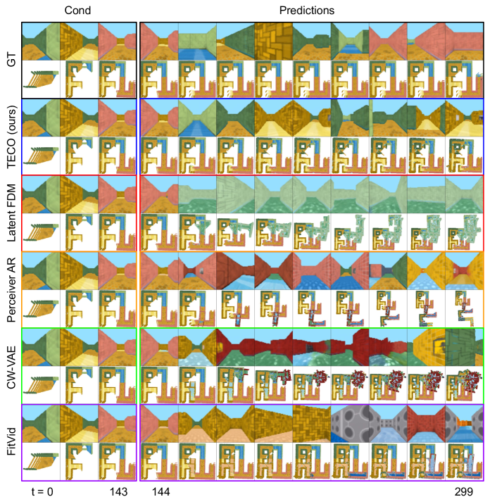
Figure 6: 3D visualization of predicted trajectories in DMLab for each model, generating 156 frames conditioned on 144. TECO is the only model that retain maze consistency with ground-truth, whereas baselines tend to extend out of the maze or create fictitious corridors that did not exist. Video predictions use only the first-person RGB frames. Refer to Section M.1 for more details on 3D evaluation. A video corresponding to this figure is available at: https://wilson1yan.github.io/teco.

4.2 Baselines

We compare against SOTA baselines selected from several different families of models: latent-variable-based variational models, autoregressive likelihood models, and diffusion models. In addition, for efficiency, we train all models on VQ codes using a pretrained VQ-GAN for each dataset. For our diffusion baseline, we follow (Rombach et al., 2022) and use a VAE instead of a VQ-GAN. Note that we do not have any GANs for our baselines, since to the best of our knowledge, there does not exist a GAN that trains on latent space instead of raw pixels, an important aspect for properly scaling to long video sequences.

Space-time Transformers We compare TECO to several variants of space-time transformers as depicted in Figure 3: VideoGPT (Yan et al., 2021) (autoregressive over space-time), Phenaki (Villegas et al., 2022) (MaskGit over space-time full attention), MaskViT (Gupta et al., 2022) (MaskGit over space-time axial attention), and Hourglass transformers (Nawrot et al., 2021) (hierarchical autoregressive over space-time). Note that we do not include the text-conditioning for Phenaki as it is irrelevant in our case. We only evaluate these models on DMLab, as Table 2 and Table 1 show that Perceiver-AR (a space-time transformer with improvements specifically for learning long dependencies) is a stronger baseline.

FitVid FitVid (Babaeizadeh et al., 2021) is a state-of-the-art variational video model based on CNNs and LSTMs that scales to complex video by leveraging efficient architectural design choices in its encoder and decoder.

Clockwork VAE CW-VAE (Saxena et al., 2021) is a variational video model that is designed to learn long-range dependencies through a hierarchy of latent variables with exponentially slower tick speeds for each new level.

Perceiver AR We use Perceiver AR (Hawthorne et al., 2022) as our AR baseline over VQ-GAN discrete latents, which has been show to be an effective generative model that can efficiently incorporate long-range sequential dependencies. Conceptually, this baseline is similar to HARP (Seo et al., 2022) with a Perceiver AR as the prior instead of a sparse transformer (Child et al., 2019). We choose Perceiver AR over other autoregressive baselines such as VideoGPT (Yan et al., 2021) or TATS (Ge et al., 2022) primarily due to the prohibitive costs of transformers when applied to tens of thousands of tokens.

Latent FDM We train a Latent FDM model for our diffusion baseline. Although FDM (Harvey et al., 2022) is originally trained on pixel observations, we also train in latent space for a more fair comparison with our method and other baselines, as training on long sequences in pixel space is too expensive. We follow LDM (Rombach et al., 2022) to separately train an autoencoder to encode each frame into a set of continuous latents.

Table 2: TECO substantially outperforms similar video generation models that use space-time transformers.

Model	FVD$\downarrow$	PSNR$\uparrow$	SSIM$\uparrow$	LPIPS$\downarrow$
TATS	156	11.1	0.296	0.468
Phenaki	725	11.0	0.202	0.474
MaskViT	76	12.4	0.360	0.435
Hourglass	110	11.7	0.335	0.458
TECO (ours)	48	21.9	0.703	0.157

4.3 Experimental Setup

Training All models are trained for 1 million iterations under fixed compute budgets allocated for each dataset (measured in TPU-v3 days) on TPU-v3 instances ranging from v3-8 to v3-128 TPU pods (similar to 4 V100s to 64 V100s) with training times of roughly 3-5 days. For DMLab, Minecraft, and Habitat we train all models on full 300 frames videos, and 100 frames for Kinetics-600. Our VQ-GANs are trained on 8 A5000 GPUs, taking about 2-4 days for each dataset, and downsample all videos to $16\times 16$ grids of discrete latents per frame regardless of original video resolution. More details on exact hyperparameters and compute budgets for each dataset can be found in Appendix N.

Evaluation

Standard methods for evaluating video prediction quality (FVD (Unterthiner et al., 2019) or per-frame metrics PSNR (Huynh-Thu & Ghanbari, 2008), SSIM (Wang et al., 2004), and LPIPS (Zhang et al., 2012)) do not measure long-consistency well. FVD is more sensitive to image fidelity, and relies on an I3D network trained on short Kinetics-600 clips. Evaluations using PSNR, SSIM, and LPIPS generally require sampling hundreds of futures and compare the sample that most accurately matches ground-truth. However, this does not align well with the goal of temporal consistency, as we would like the model to deterministically re-generate observed parts of the environment, and not accidentally generate the correct future after many samples.

Therefore, we propose a modified evaluation metric using PSNR, SSIM, and LPIPS that better measures temporal consistency in video generation by leveraging sufficient conditioning. Intuitively, if a video model is conditioned with enough information, future predictions should be approximately deterministic, meaning that only one sample should be needed to expect an accurate match with ground-truth. In the case of 3D environments, we can approximately make generation deterministic by conditioning on past frames (after the model has already seen most of the 3D environment) and actions (to remove stochasticity of movement). As such, for DMLab, Minecraft, and Habitat, we condition on 144 past frames as well as actions, and measure PSNR, SSIM, and LPIPS with 156 future ground-truth frames. However, note that per-frame metrics only capture temporal consistency, and do not capture a video model’s ability to model the stochasticity of video data. Therefore, we also compute FVD on 300 frame videos, conditioned on 36 frames (264 predicted frames). For Kinetics-600, we evaluate FVD on 100 frame videos, conditioned on 20 frames (80 predicted frames). We compute all metrics over batches of $256$ examples, averaged over 4 runs to make $1024$ total samples.

4.4 Benchmark Results

DMLab & Minecraft Table 1 shows quantitative results on the DMLab and Minecraft datasets. TECO performs the best across all metrics for both datasets when training on the full 300 frame videos. Figure 6 shows sample trajectories and 3D visualizations of the generated DMLab mazes, where TECO is able to generate more consistent 3D mazes. For both datasets, CW-VAE, FitVid, and Perceiver AR can produce sharp predictions, but do not model long-horizon context well, with per-frame metrics sharply dropping as the future prediction horizon increases as seen in Figure C.1. Latent FDM has consistent predictions, but high FVD most likely due to FVD being sensitive to high frequency errors.

Habitat Table 1 shows results for our Habitat dataset. We only evaluate our strongest baselines, Perceiver AR and Latent FDM due to the need to implement model parallelism. Because of high complexity of Habitat videos, all models generally perform equally as bad in per-frame metrics. However, TECO has significantly better FVD. Qualitatively, Latent FDM quickly collapses to blurred predictions with poor sample quality, and Perceiver AR generates high quality frames, though less temporally consistent than TECO: agents in Habitat videos navigate to far points in the scene and back whereas Perceiver AR tends to generate samples where the agent constantly turns. TECO generates traversals of a scene that match the data distribution more closely.

Kinetics-600 Table 1 shows FVD for predicting $80$ $128\times 128$ frames conditioned on $20$ for Kinetics-600. Although Kinetics-600 does not have many long-range dependencies, we found that TECO is able to produce more stable generations that degrade slower by incorporating longer contexts. In contrast, Perceiver AR tends to degrade quickly, with Latent FDM performing in between.

Sampling Speed Figure 5 reports sampling speed for all models on Minecraft. We observed similar results for the different model sizes used on other datasets. FitVid and CW-VAE are both significantly faster that other methods, but have poor sample quality. On the other end, Perceiver AR and Latent FDM can produce high quality samples, but are 20-60x slower than TECO, which has comparably fast sampling speed while retaining high sample quality.

4.5 Ablations

In this section, we perform ablations on various architectural decisions of our model. For simplicity, we evaluate our methods on short sequences of 16 frames from Something-Something-v2 (SSv2), as it provides insight into scaling our method on complex real-world data more similar to Kinetics-600 while being computationally cheaper to run.

Details can be found in the Appendix, Table F.1. We demonstrate that using VQ-latent dynamics with a MaskGit prior outperforms other formulations for latent dynamics models such as variational methods. In addition, we show that conditional encodings learn better representations for video predictions. We also ablate the codebook size, showing that although there exists an optimal codebook size, it does not matter too much as along as there are not too many codes, which may the prior more difficult to learn. Lastly, we show the benefits of DropLoss, with up to 60% faster training and a minimal increase in FVD. The benefits are greater for longer sequences, and allow video models to better account for long horizon context with little cost in performance.

4.6 Further Insights

We highlight a few key experimental insights for designing long-horizon video generation models. Further details can be found in Appendix I and Appendix G.

Trade-off between fidelity and learning long-range dependencies Given a network with fixed capacity, there exists an inherent trade-off between generating high fidelity and temporally consistent videos. We find that long-horizon information can be prioritized through bottlenecking representations, whereas allocating more computation towards higher resolution representations encourages higher fidelity. Due to TECO learning more compact representations, it achieves a better trade-off between fidelity and temporal consistency compared to our baseline models, demonstrated by better PSNR / SSIM / LPIPS, in addition to FVD.

Although frame quality saturates early-on, long-term consistency improves when training longer During training, we observe an interesting phenomenon where short-horizon metrics tend to saturate earlier on during training, while long-horizon metrics continue to improve until end of training. We hypothesize that this may be due to the likelihood objective, where modeling bits from neighboring frames is easier than learning long-horizon bits scattered throughout the video. This finding motivates the use of an efficient video architecture for TECO, which can be trained for more gradient steps given a fixed computational budget.

5 Discussion

We introduced TECO, an efficient video prediction model that leverages hundreds of frames of temporal context, as well as a comprehensive benchmark to evaluate long-horizon consistency. Our evaluation demonstrated that TECO accurately incorporates long-range context, outperforming SOTA baselines across a wide range of datasets. In addition, we introduce several difficult video datasets, which we hope make it easier to evaluate temporal consistency in future video prediction models. We identify several limitations as directions for future work:

• Although we show that PSNR, SSIM, and LPIPS can be reliable metrics to measure consistency when video models are properly conditioned, there remains room for better evaluation metrics that provide a reliable signal as the prediction horizon grows, since new parts of a scene that are generated are unlikely to correlate with ground truth.

• Our focus was on learning a compressed tokens and an expressive prior, which we combined with a simple full attention transformer as the sequence model. Leveraging prior work on efficient sequence models (Choromanski et al., 2020; Wang et al., 2020; Zhai et al., 2021; Gu et al., 2021; Hawthorne et al., 2022) would likely allow for further scaling.

• We trained all models on top of pretrained VQ-GAN codes to reduce the data dimensionality. This compression step lets us train on longer sequences at a cost of reconstruction error, which causes noticeable artifacts in Kinetics-600, such as corrupted text and incoherent faces. Although TECO can train directly on pixels, a $\ell_{2}$ loss results in slightly blurry predictions. Training directly on pixels with diffusion or GAN losses would be promising.

6 Acknowledgements

This work was in part supported by Panasonic through BAIR Commons, Darpa RACER, the Hong Kong Centre for Logistics Robotics, and BMW. In addition, we thank teh TRC program (https://sites.research.google/trc/about/) and Cirrascale Cloud Services (https://cirrascale.com/) for providing compute resources.

Table of Contents

A Sampling Process
B Samples
C Performance versus Horizon
D Performance versus Training Sequence Length
E Sampling Time
F Ablations
G Metrics During Training
H High Quality Spatio-Temporal Compression
I Trade-off Between Fidelity and Learning Long-Range Dependencies
J Full Experimental Results
K Scaling Results
L Related Work
M Dataset Details
N Hyperparameters

Appendix A Sampling Process

Given a sequence of conditioning frames, $o_{1},\dots,o_{t}$, we encode each frame using the pretrained VQ-GAN to produce $x_{1},\dots,x_{t}$, and then use the conditional encoder to compute $z_{1},\dots,z_{t}$. In order to generate the next frame, we use the temporal transformer to compute $h_{t}$, and feed it into the MaskGit dynamics prior to predict $\hat{z}_{t+1}$. Let $z_{t+1}=\hat{z}_{t+1}$ and feed it through the temporal tranformer and MaskGit to predict $\hat{z}_{t+2}$. We repeat this process until the entire trajectory is predicted, $\hat{z}_{t+1},\dots,\hat{z}_{T}$. In order to decode back into frames, we first decode into the VQ-GAN latents, and then decode to RGB using the VQ-GAN decoder. Note that generation can be completely done in latent space, and rendering back to RGB can be done in parallel over time once the latents for all timesteps are computed.

Appendix B Samples

B.1 DMLab

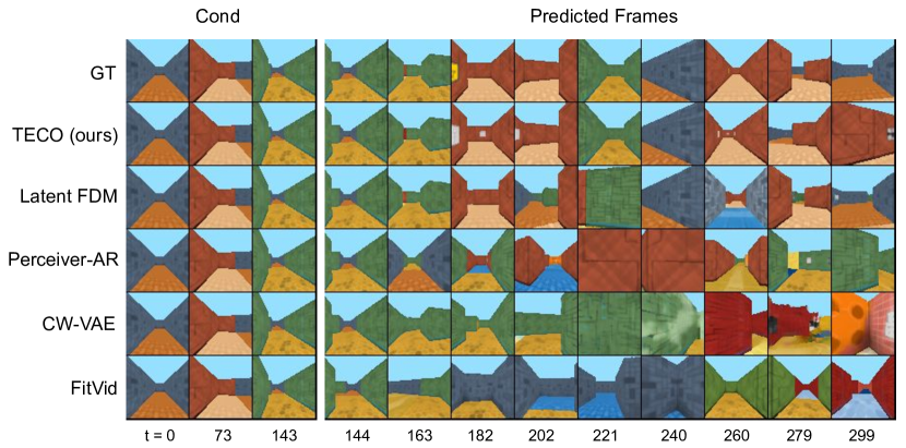
Figure B.1: 156 frames generated conditioned on 144 (action-conditioned)

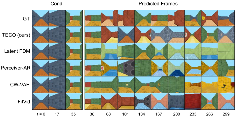
Figure B.2: 264 frames generated conditioned on 36 (no action-conditioning)

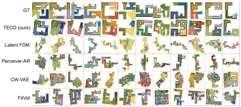
Figure B.3: 3D visualizations of the resulting generated DMLab mazes

B.2 Minecraft

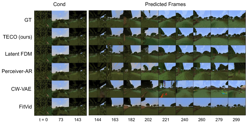
Figure B.4: 156 frames generated conditioned on 144 (action-conditioned)

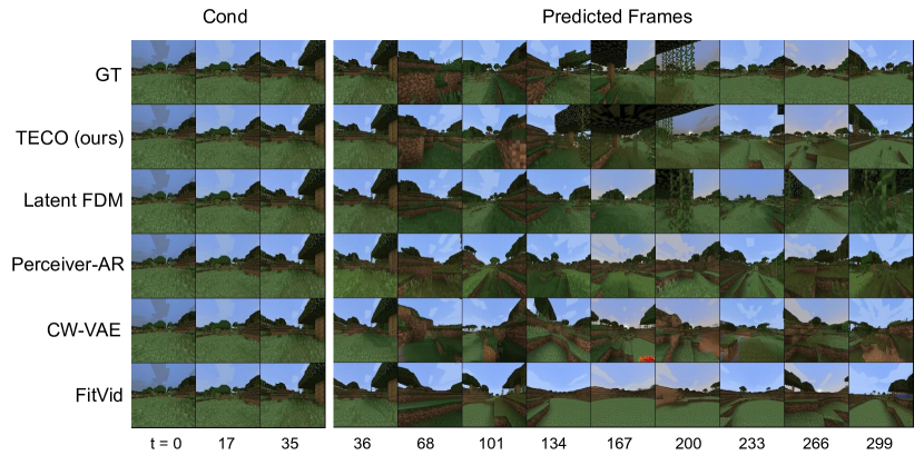
Figure B.5: 264 frames generated conditioned on 36 (action-conditioned)

B.3 Habitat

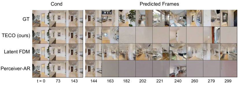
Figure B.6: 156 frames generated conditioned on 144 (action-conditioned)

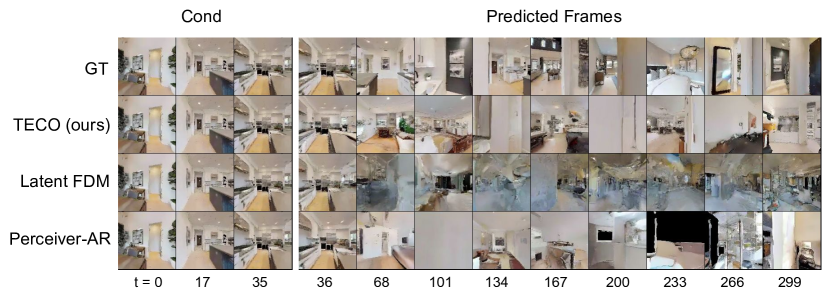
Figure B.7: 264 frames generated conditioned on 36 (no action-conditioning)

B.4 Kinetics-600

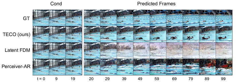
Figure B.8: 80 frames generated conditioned on 20 (no top-k sampling)

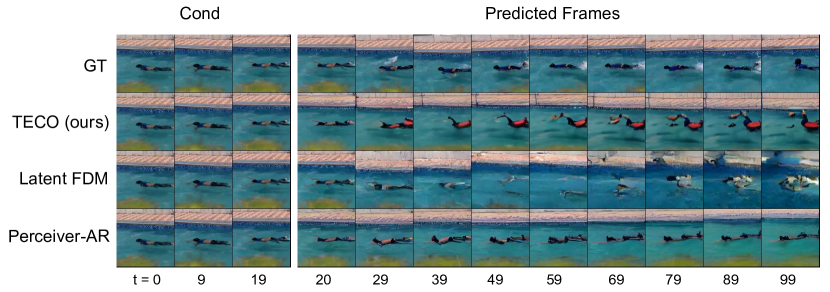
Figure B.9: 80 frames generated conditioned on 20 (with top-k sampling)

Appendix C Performance versus Horizon

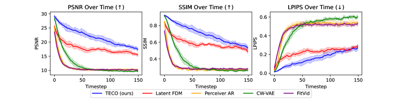
(a) DMLab

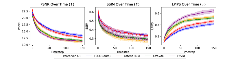
(b) Minecraft

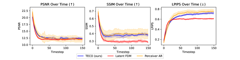
(c) Habitat

Figure C.1: All plots shows PSNR, SSIM, and LPIPS on 150 predicted frames conditioned on 144 frames. The 144 conditioned frames are not shown on the graphs and timestep 0 corresponds to the first predicted frame

Figure C.1 shows PSNR, SSIM, and LPIPS as a function of prediction horizon for each dataset. Generally, each plot reflected the corresponding aggregated metrics in Table 1. For DMLab, TECO shows much better temporal consistency for the full trajectory, with Latent FDM coming in second. CW-VAE is able retain some consistency but drops fairly quickly. Lastly, FitVid and Perceiver AR lose consistency very quickly. We see a similar trend in Minecraft, with Latent FDM coming closer in matching TECO. For Habitat, all methods generally have trouble producing consistent predictions, primarily due to the difficulty of the environment.

Appendix D Performance versus Training Sequence Length

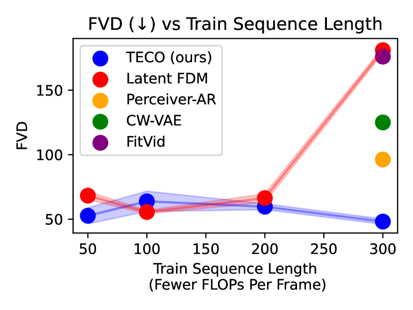
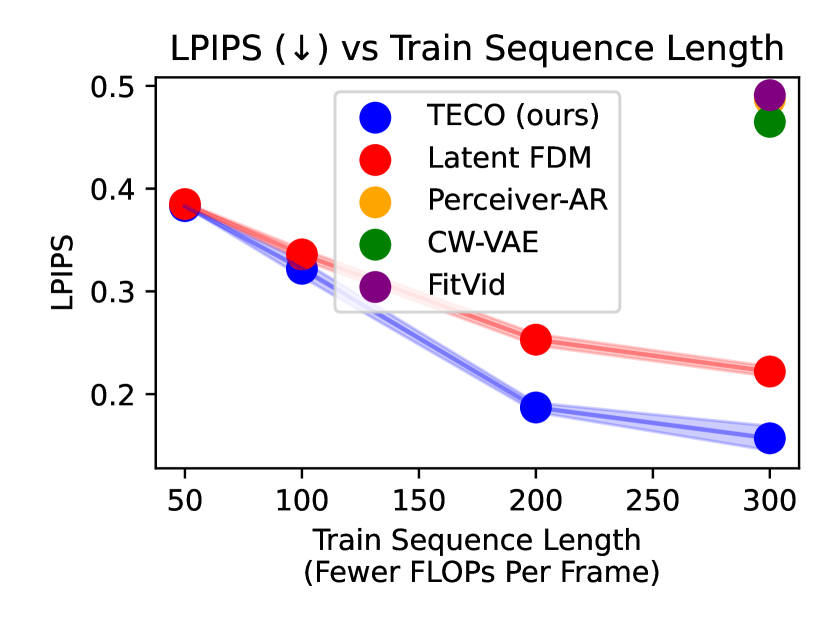
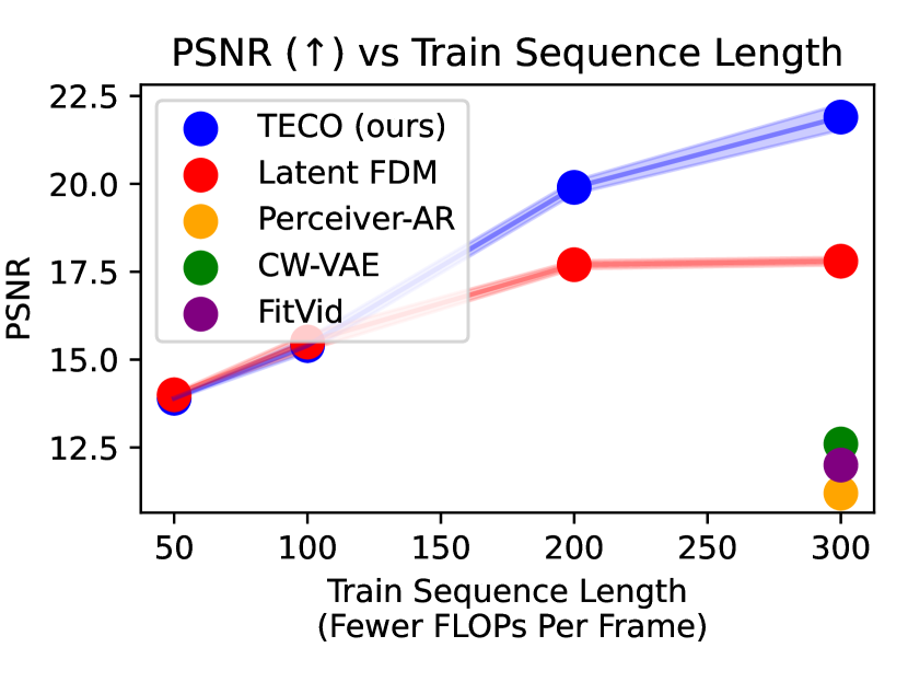
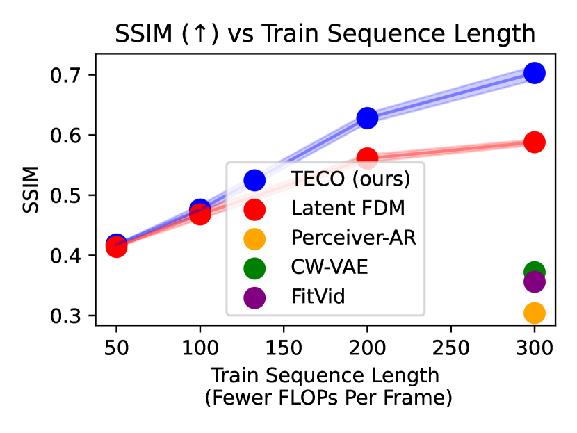
Figure D.1: DMLab

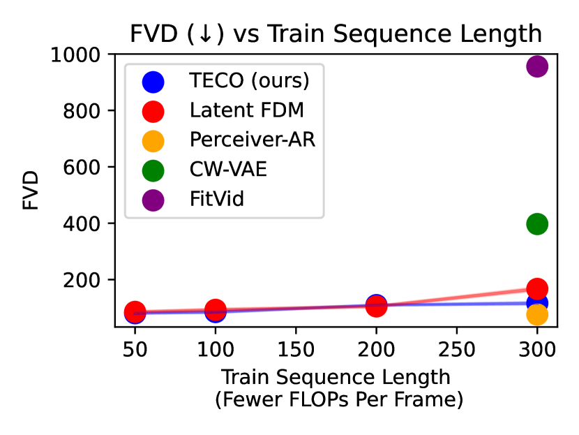
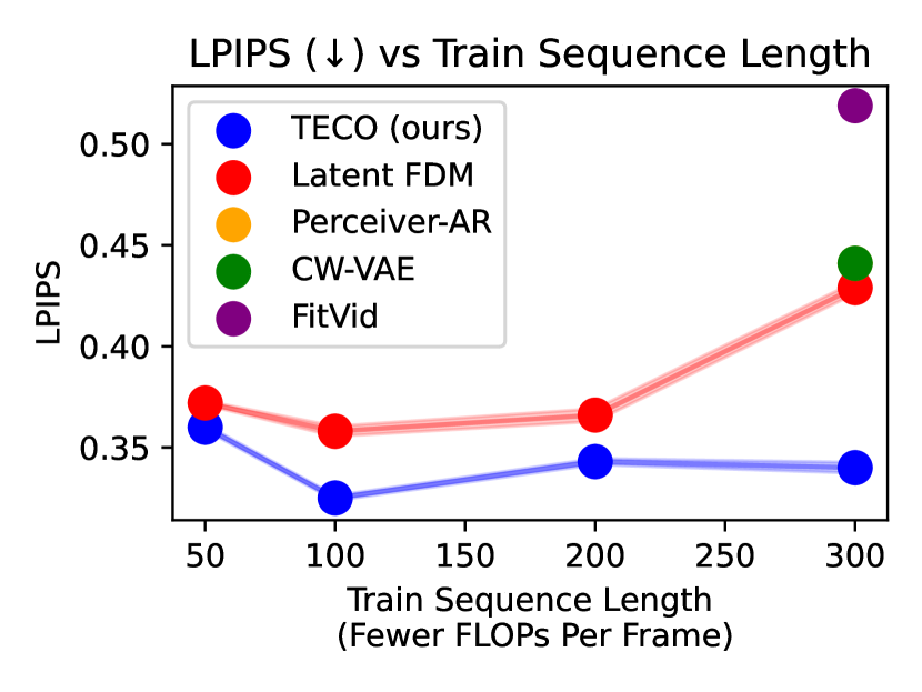
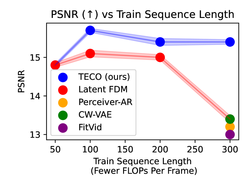
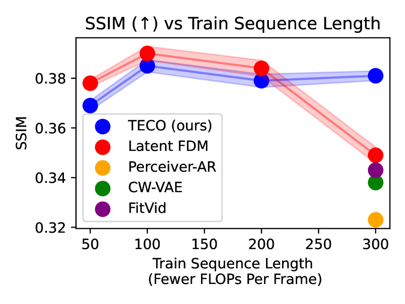
Figure D.2: Minecraft

Figure D.1 and Figure D.2 show plots comparing performance with training models on different sequence lengths. Under a fixed compute budget and batch size, training on shorter videos enables us to scale to larger models. This can also be interpreted as model capacity or FLOPs allocated per image. In general, training on shorter videos enables higher quality frames (per-image) but at a cost of worse temporal consistency due to reduced context length. We can see a very clear trend in DMLab, in that TECO is able to better scale on longer sequences, and correspondingly benefits from it. Latent FDM has trouble when training on full sequences. We hypothesize that this may be due to diffusion models being less amenable towards downsamples, it it needs to model and predict noise. In Minecraft, we see the best performance at around 50-100 training frames, where a model has higher fidelity image predictions, and also has sufficient context.

Appendix E Sampling Time

	Sampling Time per Frame (ms)
TECO (ours)	$186$
Latent FDM	$3606$
Perceiver-AR	$8443$
CW-VAE	$0.062$
FitVid	$0.074$

Appendix F Ablations

DropLoss Rate	FVD	Train Step (ms)
0.8	$187$	$125$
0.6	$186$	$143$
0.4	$184$	$155$
0.2	$184$	$167$
0.0	$182$	$182$

(a) DropLoss Rates

Posteriors	FVD
VQ (+ MaskGit prior) (ours)	$189$
OneHot (+ MaskGit prior)	$199$
OneHot (+ Block AR prior)	$209$
OneHot (+ Independent prior)	$228$
Argmax (+ MaskGit prior)	$336$

(b) Posteriors

Dynamics Prior	FVD
MaskGit (ours)	$189$
Independent	$220$
Autoregressive	$207$

(c) Prior Networks

Conditional Encoding	FVD
Yes (ours)	189
No	208

(d) Conditional Encoding

Number of Codes	FVD
64	191
256	195
1024	186
4096	200

(e) VQ Codebook Size

Table F.1: Ablations comparing alternative prior, posterior, and codebook designs

	FVD
Size	$2\times 2$	$4\times 4$
Base	204	189
Small Enc	214	191
Small Dec	232	198

(a) Encoder and Decoder

		FVD
Layers	Width	$2\times 2$	$4\times 4$
8	768	204	189
8	384	260	196
2	768	216	202

(b) Temporal Transformer

		FVD
Layers	Width	$2\times 2$	$4\times 4$
8	768	204	189
8	384	228	193
2	768	228	201

(c) MaskGit Prior

Table F.2: Ablations on scaling different parts of TECO.

	FVD ($\downarrow$)	PSNR ($\uparrow$)	SSIM ($\uparrow$)	LPIPS ($\downarrow$)	Train Step Time (ms)
TECO (ours)	$48$	$\mathbf{21.9}$	$\mathbf{0.703}$	$\mathbf{0.157}$	$\mathbf{151}$
MaskGit	$950$	$19.3$	$0.605$	$0.274$	$167$
Autoregressive	44	$20.1$	$0.640$	$0.197$	$267$

Table F.3: DMLab dataset comparisons against similar model as TECO without latent dynamics, and Maskgit or AR model on VQ-GAN tokens directly.

Table F.3 shows comparisons between TECO and alternative architectures that do not use latent dynamics. Architecturally, MaskGit and Autoregressive are very similar to TECO, with a few small changes: (1) there is no CNN decoder and (2) MaskGit and AR directly predict the VQ-GAN latents (as opposed to the learned VQ latents in TECO). In terms of training time, MaskGit and AR are a little slower since they operate on $16\times 16$ latents instead of $8\times 8$ latents for TECO. In addition, conditioning for the AR model is done using cross attention, as channel-wise concatenation does not work well due to unidirectioal masking. Both models without latent dynamics have worse temporal consistency, as well as overall sample quality. We hypothesize that TECO has better temporal consistency due to weak bottlenecking of latent representation, as a lot of time can be spent modeling likelihood of imperceptible image / video statistics. MaskGit shows very high FVD due to a tendency to collapse in later frames of prediction, which FVD is sensitive to.

Appendix G Metrics During Training

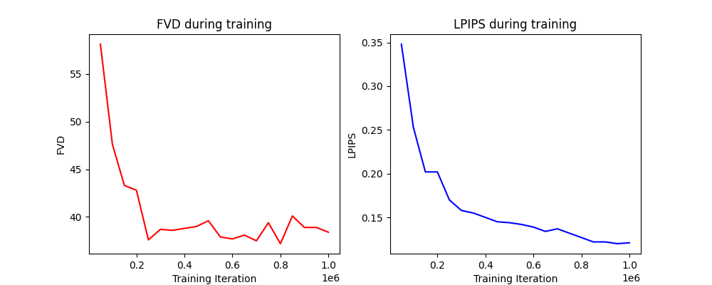
Figure G.1: Comparing FVD and LPIPS evaluation metrics over the course of training. FVD tends to saturate earlier (200k) while LPIPS keeps on improving up until 1M iterations.

Figure G.1 shows plots of FVD (over chunks of generatd 16 frame video) and LPIPS during training, evaluated at saved model checkpoints every 50k iterations over 1M iterations. We can see that although FVD (measuring frame fidelity) tends to saturate early on during training (at around 200k iterations), the long-term consistency metric (LPIPS) continues to improve until the end of training. We hypothesize that this may be due to the model first learning the ”easier bits” more local in time, and then learning long-horizon bits once the easier bits have been learned.

Appendix H High Quality Spatio-Temporal Compression

Model	Dataset	FVD$\downarrow$
TATS	DMLab	54
	Minecraft	226
TECO	DMLab	7
	Minecraft	53

Table H.1: Reconstruction FVD comparing TATS Video VQGAN to TECO

Table H.1 compares reconstruction FVD between TECO and TATS. At the same compression rate (same number of discrete codes), TECO learns far better spatio-temporal codes that TATS, with more of a difference on more visually complex scenes (Minecraft vs DMLab).

Appendix I Trade-off Between Fidelity and Learning Long-Range Dependencies

Downsample Resolution	FVD$\downarrow$	PSNR$\uparrow$	SSIM$\uparrow$	LPIPS$\downarrow$
$1\times 1$	44	20.4	0.666	0.170
$2\times 2$	38	18.6	0.597	0.221
$4\times 4$	33	17.7	0.578	0.242

Table I.1: Comparing different input resolutions to the temporal transformer

Latent FDM Arch	FVD$\downarrow$	PSNR$\uparrow$	SSIM$\uparrow$	LPIPS$\downarrow$
More downsampling + lower resolution computations	181	17.8	0.588	0.222
Less downsample + higher resolution computations	94	15.6	0.501	0.277

Table I.2: omparing different Latent FDM architectures with more computation at different resolutions

Table I.1 and Table I.2 show a trade-off between fidelity (frame or image quality) and temporal consistency (long-range dependencies) for video prediction architectures (both TECO, and Latent FDM).

Appendix J Full Experimental Results

	TPU-v3 Days	Params	FVD $\downarrow$	PSNR $\uparrow$	SSIM $\uparrow$	LPIPS $\uparrow$
TECO (ours)	$32$	169M	$\mathbf{27.5\pm 1.77}$	$\mathbf{22.4\pm 0.368}$	$\mathbf{0.709\pm 0.0119}$	$\mathbf{0.155\pm 0.00958}$
Latent FDM	$32$	31M	$181\pm 2.20$	$17.8\pm 0.111$	$0.588\pm 0.00453$	$0.222\pm 0.00493$
Perceiver-AR	$32$	30M	$96.3\pm 3.64$	$11.2\pm 0.00381$	$0.304\pm 0.0000456$	$0.487\pm 0.00123$
CW-VAE	$32$	111M	$125\pm 7.95$	$12.6\pm 0.0585$	$0.372\pm 0.000330$	$0.465\pm 0.00156$
FitVid	$32$	165M	$176\pm 4.86$	$12.0\pm 0.0126$	$0.356\pm 0.00171$	$0.491\pm 0.00108$

Table J.1: DMLab

	TPU-v3 Days	Params	FVD $\downarrow$	PSNR $\uparrow$	SSIM $\uparrow$	LPIPS $\uparrow$
TECO (ours)	$80$	274M	$116\pm 5.08$	$\mathbf{15.4\pm 0.0603}$	$\mathbf{0.381\pm 0.00192}$	$\mathbf{0.340\pm 0.00264}$
Latent FDM	$80$	33M	$167\pm 6.26$	$13.4\pm 0.0904$	$0.349\pm 0.00327$	$0.429\pm 0.00284$
Perceiver-AR	$80$	166M	$\mathbf{76.3\pm 1.72}$	$13.2\pm 0.0711$	$0.323\pm 0.00336$	$0.441\pm 0.00207$
CW-VAE	$80$	140M	$397\pm 15.5$	$13.4\pm 0.0610$	$0.338\pm 0.00274$	$0.441\pm 0.00367$
FitVid	$80$	176M	$956\pm 15.8$	$13.0\pm 0.00895$	$0.343\pm 0.00380$	$0.519\pm 0.00367$

Table J.2: Minecraft

	TPU-v3 Days	Params	FVD $\downarrow$	PSNR $\uparrow$	SSIM $\uparrow$	LPIPS $\uparrow$
TECO (ours)	$275$	386M	$\mathbf{76.3\pm 1.72}$	$\mathbf{12.8\pm 0.0139}$	$0.363\pm 0.00122$	$0.604\pm 0.00451$
Latent FDM	$275$	87M	$433\pm 2.67$	$12.5\pm 0.0121$	$0.311\pm 0.000829$	$\mathbf{0.582\pm 0.000492}$
Perceiver-AR	$275$	200M	$164\pm 12.6$	$\mathbf{12.8\pm 0.0423}$	$\mathbf{0.405\pm 0.00248}$	$0.676\pm 0.00282$

Table J.3: Habitat

	TPU-v3 Days	Params	FVD $\downarrow$
TECO (ours)	$640$	1.09B	$649\pm 16.5$
Latent FDM	$640$	831M	$960\pm 52.7$
Perceiver-AR	$640$	1.06B	$\mathbf{607\pm 6.98}$

(a) Using top-k sampling for Perceiver AR and TECO

	TPU-v3 Days	Params	FVD $\downarrow$
TECO (ours)	$640$	1.09B	$\mathbf{799\pm 23.4}$
Latent FDM	$640$	831M	$960\pm 52.7$
Perceiver-AR	$640$	1.06B	$1022\pm 32.4$

(b) No top-k sampling

Table J.4: Kinetics

Figure J.1: FVD on Kinetics-600 with different top-k values for Perceiver-AR and TECO

Appendix K Scaling Results

	TPU-v3 Days	Train Seq Len	Params	FVD $\downarrow$	PSNR $\uparrow$	SSIM $\uparrow$	LPIPS $\downarrow$
TECO (ours)	$32$	300	169M	$\mathbf{48.2\pm 2.02}$	$\mathbf{21.9\pm 0.368}$	$\mathbf{0.703\pm 0.0114}$	$\mathbf{0.157\pm 0.0119}$
		200	169M	$59.7\pm 2.29$	$19.9\pm 0.186$	$0.628\pm 0.00821$	$0.187\pm 0.00460$
		100	86M	$63.9\pm 7.84$	$15.4\pm 0.199$	$0.476\pm 0.00745$	$0.322\pm 0.00792$
		50	195M	$52.7\pm 6.23$	$13.9\pm 0.0311$	$0.418\pm 0.000659$	$0.383\pm 0.000302$
Latent FDM	$32$	300	31M	$181\pm 2.20$	$17.8\pm 0.111$	$0.588\pm 0.00453$	$0.222\pm 0.00493$
		200	62M	$66.4\pm 3.31$	$17.7\pm 0.114$	$0.561\pm 0.00623$	$0.253\pm 0.00550$
		100	80M	$55.6\pm 1.36$	$15.5\pm 0.233$	$0.468\pm 0.00776$	$0.336\pm 0.00511$
		50	110M	$68.3\pm 3.19$	$14.0\pm 0.0445$	$0.414\pm 0.424$	$0.385\pm 0.00151$

Table K.1: DM Lab scaling

	TPU-v3 Days	Train Seq Len	Params	FVD $\downarrow$	PSNR $\uparrow$	SSIM $\uparrow$	LPIPS $\downarrow$
TECO (ours)	$80$	300	274M	$116\pm 5.08$	$15.4\pm 0.0603$	$0.381\pm 0.00192$	$0.340\pm 0.00264$
		200	261M	$109.5\pm 1.46$	$15.4\pm 0.0906$	$0.379\pm 0.00263$	$0.343\pm 0.00148$
		100	257M	$85.1\pm 4.09$	$\mathbf{15.7\pm 0.0516}$	$0.385\pm 0.00244$	$\mathbf{0.325\pm 0.00121}$
		50	140M	$80.7\pm 1.42$	$14.8\pm 0.0404$	$0.369\pm 0.00197$	$0.360\pm 0.00133$
Latent FDM	$80$	300	33M	$167\pm 6.26$	$13.4\pm 0.0904$	$0.349\pm 0.00327$	$0.429\pm 0.00284$
		200	80M	$104.9\pm 3.21$	$15.0\pm 0.0701$	$0.384\pm 0.00320$	$0.366\pm 0.00311$
		100	69M	$92.8\pm 4.40$	$15.1\pm 0.0866$	$\mathbf{0.390\pm 0.00281}$	$0.358\pm 0.00250$
		50	186M	$85.6\pm 2.25$	$14.8\pm 0.0578$	$0.378\pm 0.00144$	$0.372\pm 0.000966$

Table K.2: Minecraft scaling

Appendix L Related Work

Video Generation Prior video generation methods can be divided into a few classes of models: variational models, exact likelihood models, and GANs. SV2P (Babaeizadeh et al., 2017), SVP (Denton & Fergus, 2018), SVG (Villegas et al., 2019), and FitVid (Babaeizadeh et al., 2021) are variational video generation methods models videos through stochastic latent dynamics, optimized using the ELBO (Kingma & Welling, 2013) objective extended in time. SAVP (Lee et al., 2018) adds an adversarial (Goodfellow et al., 2014) loss to encourage more realistic and high-fidelity generation quality. Diffusion models (Ho et al., 2020; Sohl-Dickstein et al., 2014) have recently emerged as a powerful class of variational generative models which learn to iteratively denoise an initial noise sample to generate high-quality images. There have been several recent works that extend diffusion models to video, through temporal attention (Ho et al., 2022; Harvey et al., 2022), 3D convolutions (Höppe et al., 2022), or channel stacking (Voleti et al., 2022). Unlike variational models, autoregressive models (AR) and flows (Kumar et al., 2019) model videos by optimizing exact likelihood. Video Pixel Networks (Kalchbrenner et al., 2017) and Subscale Video Transformers (Weissenborn et al., 2019) autoregressively model each pixel. For more compute efficient training, some prior methods (Yan et al., 2021; Le Moing et al., 2021; Seo et al., 2022; Rakhimov et al., 2020; Walker et al., 2021) propose to learn an AR model in a spatio-temporally compressed latent space of a discrete autoencoder, which has shown to be orders of magnitudes more efficient compared to pixel-based methods. Instead of a VQ-GAN, (Le Moing et al., 2021), learns a frame conditional autoencoder through a flow mechanism. Lastly, GANs (Goodfellow et al., 2014) offer an alternative method to training video models. MoCoGAN (Tulyakov et al., 2018) generates videos by disentangling style and motion. MoCoGAN-HD (Tian et al., 2021) can efficiently extend to larger resolutions by learning to navigate the latent space of a pretrained image generator. TGANv2 (Saito & Saito, 2018), DVD-GAN (Clark et al., 2019), StyleGAN-V (Skorokhodov et al., 2021), and TrIVD-GAN (Luc et al., 2020) introduce various methods to scale to complex video, such as proposing sparse training, or more efficient discriminator design.

The main focus of this work lies with video prediction, a specific interpretation of conditional video generation. Most prior methods are trained autoregressive in time, so they can be easily extended to video prediction. Video Diffusion, although trained unconditionally proposes reconstruction guidance for prediction. GANs generally require training a separate model for video prediction. However, some methods such as MoCoGAN-HD and DI-GAN can approximate frame conditioning by inverting the generator to compute a corresponding latent for a frame.

Long-Horizon Video Generation CW-VAE (Saxena et al., 2021) learns a hierarchy of stochastic latents to better model long term temporal dynamics, and is able to generate videos with long-term consistency for hundreds of frames. TATS (Ge et al., 2022) extends VideoGPT which allows for sampling of arbitrarily long videos using a sliding window. In addition, TATs and CogVideo (Hong et al., 2022) propose strided sampling as a simple method to incorporate longer horizon contexts. StyleGAN-V (Skorokhodov et al., 2021) and DI-GAN (Yu et al., 2022) learn continuous-time representations for videos which allow for sampling of arbitrary long videos as well. (Brooks et al., 2022) proposes an efficient video GAN architecture that is able to generate high resolution videos of 128 frames on complex video data for dynamic scenes and horseback riding. FDM (Harvey et al., 2022) proposes a diffusion model that is trained to be able to flexibly condition on a wide range of sampled frames to better incorporate context of arbitrarily long videos. (Lee et al., 2021) is able to leverage a hierarchical prediction framework using semantic segmentations to generate long videos.

Long-Horizon Video Understanding Outside of generative modeling, prior work such as MeMViT (Wu et al., 2022) and Vis4mer (Mohaiminul Islam & Bertasius, 2022) introduce architectures for modeling long-horizon dependencies in videos.

Appendix M Dataset Details

M.1 DMLab

We generate random $7\times 7$ mazes split into four quadrants, with each quadrant containing a random combination of wall and floor textures. We generate 40k trajectories of 300 frames, each $64\times 64$ images. Actions in this environment consist of $20^{\circ}$ left turn, $20^{\circ}$ right turn, and walk forward. In order to maximally traverse the maze, we code an agent that traverses to the furthest unvisited point in the maze, with some added noise for stochasticity. Since the maze is a grid, we can easily hard-code a navigation policy to move to any specified point in the maze.

For 3D visualizations, we also collect depth, camera intrinsics and camera extrinsics (pose) for each timestep. Given this information, we can project RGB points into a 3D coordinate space and reconstruct the maze as a 3D pointcloud. Note that since videos are generated only using RGB as input, they do not have groundtruth depth and pose. Therefore, we train depth and pose estimators that are used during evaluation. Specifically, we train a depth estimator to map from RGB frame to depth, and a pose estimator that takes in two adjacent RGB frames and predicts the relative change in orientation. During evaluation, we are given an initial ground truth orientation that we apply sequentially to predicted frames.

Although the GQN Mazes (Eslami et al., 2018) already exists as a video prediction dataset, it is difficult to properly measure temporal consistency. The 3D scenes are relatively simple, and it does not have actions to help reduce stochasticity in using metrics such as PSNR, SSIM, and LPIPS. As a result, FVD is the reliable metric used in GQN Mazes, but tends to be sensitive to noise in video predictions. In addition, we perform 3D visualizations using our dataset that are not possible with GQN Mazes.

M.2 Minecraft

We generate 200k trajectories (each of a different Minecraft world) of 300 $128\times 128$ frames in the Minecraft marsh biome. We hardcode an agent to randomly traverse the surroundings by taking left, right, and forward actions with different probabilities. In addition, we let the agent constantly jump, which we found to help traverse simple hills, and prevent itself from drowning. We specifically chose the marsh biome, as it contains hilly turns with sparse collections of trees that act as clear landmarks for consistent generation. Forest and jungle biomes tend to be too dense for any meanginfully clear consistency, as all surroundings look nearly identical. On the other hand, plains biomes had the opposite issue where the surroundings were completely flat. Mountain biomes were too hilly and difficult to traverse.

We opt to introduce an alternative to the MineRL Navigate (Guss et al., 2019) since this dataset primarily consists of human demonstrations of people navigating to specific points. This means that trajectories usually follow a relatively straight line, so there are not many long-term dependencies in this dataset, as only a few past frames of context are necessary for prediction.

M.3 Habitat

Habitat is a 3D simulator that can render realistic trajectories in scans of 3D scenes. We compile roughly 1400 3D scans from HM3D (Ramakrishnan et al., 2021), MatterPort3D (Chang et al., 2017) and Gibson (Xia et al., 2018), and generate a total of 200k trajectories of $300$ $128\times 128$ frames. We use the in-built path traversal algorithm provided in Habitat to construct action trajectories that allow our agent to move between randomly sampled locations in the 3D scene. Similar to Minecraft and DMLab, the agent action space consists of left turn, right turn, and move forward.

Appendix N Hyperparameters

N.1 VQ-GAN & VAE

	DMLab / Minecraft	Habitat / Kinetics-600
GPU Days	16	32
Resolution	64 / 128	128
Batch Size	64	64
LR	$3\times 10^{-4}$	$3\times 10^{-4}$
Num Res Blocks	2	2
Attention Resolutions	16	16
Channel Mult	1,2,2,2	1,2,3,4
Base Channels	128	128
Latent Size (VQ-GAN)	$16\times 16$	$16\times 16$
Embedding Dim (VQ-GAN)	256	256
Codebook Size (VQ-GAN)	1024	8192
Latent Size (VAE)	$16\times 16\times 4$	$16\times 16\times 8$

N.2 TECO

Hyperparameters		DMLab	Minecraft	Habitat	Kinetics-600
	TPU-v3 Days	32	80	275	640
	Params	169M	274M	386M	1.09B
	Resolution	64	128	128	128
	Batch Size	32	32	32	32
	Sequence Length	300	300	300	100
	LR	$1\times 10^{-4}$	$1\times 10^{-4}$	$1\times 10^{-4}$	$1\times 10^{-4}$
	LR Schedule	cosine	cosine	cosine	cosine
	Warmup Steps	10k	10k	10k	10k
	Total Training Steps	1M	1M	1M	1M
	DropLoss Rate	0.9	0.9	0.9	0.9
Encoder	Depths	256, 512	256, 512	256, 512	256, 512
	Blocks	2	4	4	8
Codebook	Size	1024	1024	1024	1024
	Embedding Dim	32	32	32	32
Decoder	Depths	256, 512	256, 512	256, 512	256, 512
	Blocks	4	8	8	10
Temporal Transformer	Downsample Factor	8	8	4	2
	Hidden Dim	1024	1024	1024	1536
	Feedforward Dim	4096	4096	4096	6144
	Heads	16	16	16	24
	Layers	8	12	8	24
	Dropout	0	0	0	0
MaskGit	Mask Schedule	cosine	cosine	cosine	cosine
	Hidden Dim	512	768	1024	1024
	Feedforward Dim	2048	3072	4096	4096
	Heads	8	12	16	16
	Layers	8	6	16	24
	Dropout	0	0	0	0

		Train Sequence Length (Fewer FLOPs per Frame)
Hyperparameters		300	200	100	50
	TPU-v3 Days	32	32	32	32
	Params	169M	169M	86M	195M
	Resolution	64	64	64	64
	Batch Size	32	32	32	32
	LR	$1\times 10^{-4}$	$1\times 10^{-4}$	$1\times 10^{-4}$	$1\times 10^{-4}$
	LR Schedule	cosine	cosine	cosine	cosine
	Warmup Steps	10k	10k	10k	10k
	Total Training Steps	1M	1M	1M	1M
	DropLoss Rate	0.9	0.85	0.85	0.85
Encoder	Depths	256, 512	256, 512	256, 512	256, 512
	Blocks	2	2	2	2
Codebook	Size	1024	1024	1024	1024
	Embedding Dim	32	32	32	32
Decoder	Depths	256, 512	256, 512	256, 512	256, 512
	Blocks	4	4	4	4
Temporal Transformer	Downsample Factor	8	8	2	2
	Hidden Dim	1024	1024	512	1024
	Feedforward Dim	4096	4096	2048	4096
	Heads	16	16	8	16
	Layers	8	8	8	8
	Dropout	0	0	0	0
MaskGit	Mask Schedule	cosine	cosine	cosine	cosine
	Hidden Dim	512	512	512	768
	Feedforward Dim	2048	2048	2048	3072
	Heads	8	8	8	12
	Layers	8	8	8	8
	Dropout	0	0	0	0

Table N.1: Hyperparameters for scaling TECO on DMLab

		Train Sequence Length (Fewer FLOPs per Frame)
Hyperparameters		300	200	100	50
	TPU-v3 Days	80	80	80	80
	Params	274M	261M	257M	140M
	Resolution	128	128	128	128
	Batch Size	32	32	32	32
	LR	$1\times 10^{-4}$	$1\times 10^{-4}$	$1\times 10^{-4}$	$1\times 10^{-4}$
	LR Schedule	cosine	cosine	cosine	cosine
	Warmup Steps	10k	10k	10k	10k
	Total Training Steps	1M	1M	1M	1M
	DropLoss Rate	0.9	0.85	0.25	0.25
Encoder	Depths	256, 512	256, 512	256, 512	256, 512
	Blocks	4	4	4	4
Codebook	Size	1024	1024	1024	1024
	Embedding Dim	32	32	32	32
Decoder	Depths	256, 512	256, 512	256, 512	256, 512
	Blocks	8	8	8	8
Temporal Transformer	Downsample Factor	8	4	2	2
	Hidden Dim	1024	1024	1024	512
	Feedforward Dim	4096	4096	4096	2048
	Heads	16	16	16	8
	Layers	12	12	12	12
	Dropout	0	0	0	0
MaskGit	Mask Schedule	cosine	cosine	cosine	cosine
	Hidden Dim	768	768	768	768
	Feedforward Dim	3072	3072	3072	3072
	Heads	12	12	12	12
	Layers	6	6	6	8
	Dropout	0	0	0	0

Table N.2: Hyperparameters for scaling TECO on Minecraft

N.3 Latent FDM

Hyperparameters	DMLab	Minecraft	Habitat	Kinetics-600
TPU-v3 Days	32	80	275	640
Params	31M	33M	87M	831M
Resolution	64	128	128	128
Batch Size	32	32	32	32
LR	$1\times 10^{-4}$	$1\times 10^{-4}$	$1\times 10^{-4}$	$1\times 10^{-4}$
LR Schedule	cosine	cosine	cosine	cosine
Optimizer	Adam	Adam	Adam	Adam
Warmup Steps	10k	10k	10k	10k
Total Training Steps	1M	1M	1M	1M
Base Channels	128	128	128	256
Num Res Blocks	1,1,1,2	1,1,2,2	1,2,2,4	2,2,2,2
Head Dim	64	64	64	64
Attention Resolutions	4,2	4,2	4,2	8,4,2
Dropout	0	0	0	0
Channel Mult	1,1,1,2	1,2,2,2	1,2,2,4	1,2,3,8

Table N.3: Hyperparameters for Latent FDM

	Train Sequence Length (Fewer FLOPs per Frame)
Hyperparameters	300	200	100	50
TPU-v3 Days	32	32	32	32
Params	31M	62M	80M	110M
Resolution	64	64	64	64
Batch Size	32	32	32	32
LR	$1\times 10^{-4}$	$1\times 10^{-4}$	$1\times 10^{-4}$	$1\times 10^{-4}$
LR Schedule	cosine	cosine	cosine	cosine
Optimizer	Adam	Adam	Adam	Adam
Warmup Steps	10k	10k	10k	10k
Total Training Steps	1M	1M	1M	1M
Base Channels	128	128	128	192
Num Res Blocks	1,1,1,2	1,1,2,2,4	2,2,2,2	3,3,3,3
Head Dim	64	64	64	64
Attention Resolutions	4,2	4,1	4,2	8,4,2
Dropout	0	0	0	0
Channel Mult	1,1,1,2	1,1,2,2,4	1,2,3,4	1,2,3,4

Table N.4: Hyperparameters for scaling Latent FDM on DMLab

	Train Sequence Length (Fewer FLOPs per Frame)
Hyperparameters	300	200	100	50
TPU-v3 Days	80	80	80	80
Params	33M	80M	69M	186M
Resolution	128	128	128	128
Batch Size	32	32	32	32
LR	$1\times 10^{-4}$	$1\times 10^{-4}$	$1\times 10^{-4}$	$1\times 10^{-4}$
LR Schedule	cosine	cosine	cosine	cosine
Optimizer	Adam	Adam	Adam	Adam
Warmup Steps	10k	10k	10k	10k
Total Training Steps	1M	1M	1M	1M
Base Channels	128	128	128	192
Num Res Blocks	1,1,2,2	2,2,2,2	3,3,3,3	2,2,2,2
Head Dim	64	64	64	64
Attention Resolutions	4,2	4,2	8,4,2	8,4,2
Dropout	0	0	0	0
Channel Mult	1,2,2,2	1,2,3,4	1,2,2,3	1,2,3,4

Table N.5: Hyperparameters for scaling Latent FDM on Minecraft

N.4 CW-VAE

Hyperparameters		DMLab	Minecraft
	TPU-v3 Days	32	80
	Params	111M	140M
	Resolution	64	128
	Batch Size	32	32
	LR	$1\times 10^{-4}$	$1\times 10^{-4}$
	LR Schedule	cosine	cosine
	Optimizer	Adam	Adam
	Warmup Steps	10k	10k
	Total Training Steps	1M	1M
Encoder	Kernels	4,4,4	4,4,4
	Filters	256,512,1024	256,512,1024
Decoder	Depths	256,512	256,512
	Blocks	4	8
Dynamics	Levels	3	3
	Abs Factor	6	6
	Enc Dense Layers	3	3
	Enc Dense Embed	1024	1024
	Cell Stoch Size	128	256
	Cell Deter Size	1024	1024
	Cell Embed Size	1024	1024
	Cell Min Stddev	0.001	0.001

Table N.6: Hyperparameters for CW-VAE

N.5 FitVid

Hyperparameters	DMLab	Minecraft
TPU-v3 Days	32	80
Params	165M	176M
Resolution	64	128
Batch Size	32	32
LR	$1\times 10^{-4}$	$1\times 10^{-4}$
LR Schedule	cosine	cosine
Optimizer	Adam	Adam
Warmup Steps	10k	10k
Total Training Steps	1M	1M
g Dim	256	256
RNN Size	512	768
z Dim	64	128
Filters	128,128,256,512	128,128,256,512

Table N.7: Hyperparameters for FitVid

References

- Babaeizadeh et al. (2017) Babaeizadeh, M., Finn, C., Erhan, D., Campbell, R. H., and Levine, S. Stochastic variational video prediction. arXiv preprint arXiv:1710.11252, 2017.
- Babaeizadeh et al. (2021) Babaeizadeh, M., Saffar, M. T., Nair, S., Levine, S., Finn, C., and Erhan, D. Fitvid: Overfitting in pixel-level video prediction. arXiv preprint arXiv:2106.13195, 2021.
- Beattie et al. (2016) Beattie, C., Leibo, J. Z., Teplyashin, D., Ward, T., Wainwright, M., Küttler, H., Lefrancq, A., Green, S., Valdés, V., Sadik, A., et al. Deepmind lab. arXiv preprint arXiv:1612.03801, 2016.
- Bengio (2013) Bengio, Y. Estimating or propagating gradients through stochastic neurons. arXiv preprint arXiv:1305.2982, 2013.
- Brooks et al. (2022) Brooks, T., Hellsten, J., Aittala, M., Wang, T.-C., Aila, T., Lehtinen, J., Liu, M.-Y., Efros, A. A., and Karras, T. Generating long videos of dynamic scenes. arXiv preprint arXiv:2206.03429, 2022.
- Carreira & Zisserman (2017) Carreira, J. and Zisserman, A. Quo vadis, action recognition? a new model and the kinetics dataset. In proceedings of the IEEE Conference on Computer Vision and Pattern Recognition, pp. 6299–6308, 2017.
- Chang et al. (2017) Chang, A., Dai, A., Funkhouser, T., Halber, M., Niessner, M., Savva, M., Song, S., Zeng, A., and Zhang, Y. Matterport3d: Learning from rgb-d data in indoor environments. arXiv preprint arXiv:1709.06158, 2017.
- Chang et al. (2022) Chang, H., Zhang, H., Jiang, L., Liu, C., and Freeman, W. T. Maskgit: Masked generative image transformer. In Proceedings of the IEEE/CVF Conference on Computer Vision and Pattern Recognition, pp. 11315–11325, 2022.
- Child et al. (2019) Child, R., Gray, S., Radford, A., and Sutskever, I. Generating long sequences with sparse transformers. arXiv preprint arXiv:1904.10509, 2019.
- Choromanski et al. (2020) Choromanski, K., Likhosherstov, V., Dohan, D., Song, X., Gane, A., Sarlos, T., Hawkins, P., Davis, J., Mohiuddin, A., Kaiser, L., et al. Rethinking attention with performers. arXiv preprint arXiv:2009.14794, 2020.
- Clark et al. (2019) Clark, A., Donahue, J., and Simonyan, K. Adversarial video generation on complex datasets, 2019.
- Dai et al. (2019) Dai, Z., Yang, Z., Yang, Y., Carbonell, J., Le, Q. V., and Salakhutdinov, R. Transformer-xl: Attentive language models beyond a fixed-length context. arXiv preprint arXiv:1901.02860, 2019.
- Denton & Fergus (2018) Denton, E. and Fergus, R. Stochastic video generation with a learned prior. arXiv preprint arXiv:1802.07687, 2018.
- Eslami et al. (2018) Eslami, S. A., Jimenez Rezende, D., Besse, F., Viola, F., Morcos, A. S., Garnelo, M., Ruderman, A., Rusu, A. A., Danihelka, I., Gregor, K., et al. Neural scene representation and rendering. Science, 360(6394):1204–1210, 2018.
- Esser et al. (2021) Esser, P., Rombach, R., and Ommer, B. Taming transformers for high-resolution image synthesis. In Proceedings of the IEEE/CVF Conference on Computer Vision and Pattern Recognition, pp. 12873–12883, 2021.
- Ge et al. (2022) Ge, S., Hayes, T., Yang, H., Yin, X., Pang, G., Jacobs, D., Huang, J.-B., and Parikh, D. Long video generation with time-agnostic vqgan and time-sensitive transformer. arXiv preprint arXiv:2204.03638, 2022.
- Goodfellow et al. (2014) Goodfellow, I., Pouget-Abadie, J., Mirza, M., Xu, B., Warde-Farley, D., Ozair, S., Courville, A., and Bengio, Y. Generative adversarial nets. In Advances in neural information processing systems, pp. 2672–2680, 2014.
- Gu et al. (2021) Gu, A., Goel, K., and Ré, C. Efficiently modeling long sequences with structured state spaces. arXiv preprint arXiv:2111.00396, 2021.
- Gupta et al. (2022) Gupta, A., Tian, S., Zhang, Y., Wu, J., Martín-Martín, R., and Fei-Fei, L. Maskvit: Masked visual pre-training for video prediction. arXiv preprint arXiv:2206.11894, 2022.
- Guss et al. (2019) Guss, W. H., Houghton, B., Topin, N., Wang, P., Codel, C., Veloso, M., and Salakhutdinov, R. Minerl: A large-scale dataset of minecraft demonstrations. arXiv preprint arXiv:1907.13440, 2019.
- Harvey et al. (2022) Harvey, W., Naderiparizi, S., Masrani, V., Weilbach, C., and Wood, F. Flexible diffusion modeling of long videos. arXiv preprint arXiv:2205.11495, 2022.
- Hawthorne et al. (2022) Hawthorne, C., Jaegle, A., Cangea, C., Borgeaud, S., Nash, C., Malinowski, M., Dieleman, S., Vinyals, O., Botvinick, M., Simon, I., et al. General-purpose, long-context autoregressive modeling with perceiver ar. arXiv preprint arXiv:2202.07765, 2022.
- Ho et al. (2020) Ho, J., Jain, A., and Abbeel, P. Denoising diffusion probabilistic models. arXiv preprint arXiv:2006.11239, 2020.
- Ho et al. (2022) Ho, J., Salimans, T., Gritsenko, A., Chan, W., Norouzi, M., and Fleet, D. J. Video diffusion models. arXiv preprint arXiv:2204.03458, 2022.
- Hong et al. (2022) Hong, W., Ding, M., Zheng, W., Liu, X., and Tang, J. Cogvideo: Large-scale pretraining for text-to-video generation via transformers. arXiv preprint arXiv:2205.15868, 2022.
- Höppe et al. (2022) Höppe, T., Mehrjou, A., Bauer, S., Nielsen, D., and Dittadi, A. Diffusion models for video prediction and infilling. arXiv preprint arXiv:2206.07696, 2022.
- Hutchins et al. (2022) Hutchins, D., Schlag, I., Wu, Y., Dyer, E., and Neyshabur, B. Block-recurrent transformers. arXiv preprint arXiv:2203.07852, 2022.
- Huynh-Thu & Ghanbari (2008) Huynh-Thu, Q. and Ghanbari, M. Scope of validity of psnr in image/video quality assessment. Electronics letters, 44(13):800–801, 2008.
- Kalchbrenner et al. (2017) Kalchbrenner, N., Oord, A., Simonyan, K., Danihelka, I., Vinyals, O., Graves, A., and Kavukcuoglu, K. Video pixel networks. In International Conference on Machine Learning, pp. 1771–1779. PMLR, 2017.
- Kingma & Welling (2013) Kingma, D. P. and Welling, M. Auto-encoding variational Bayes. Proceedings of the 2nd International Conference on Learning Representations, 2013.
- Kumar et al. (2019) Kumar, M., Babaeizadeh, M., Erhan, D., Finn, C., Levine, S., Dinh, L., and Kingma, D. Videoflow: A flow-based generative model for video. arXiv preprint arXiv:1903.01434, 2(5):3, 2019.
- Le Moing et al. (2021) Le Moing, G., Ponce, J., and Schmid, C. Ccvs: Context-aware controllable video synthesis. Advances in Neural Information Processing Systems, 34, 2021.
- Lee et al. (2018) Lee, A. X., Zhang, R., Ebert, F., Abbeel, P., Finn, C., and Levine, S. Stochastic adversarial video prediction. arXiv preprint arXiv:1804.01523, 2018.
- Lee et al. (2022) Lee, D., Kim, C., Kim, S., Cho, M., and Han, W.-S. Draft-and-revise: Effective image generation with contextual rq-transformer. arXiv preprint arXiv:2206.04452, 2022.
- Lee et al. (2021) Lee, W., Jung, W., Zhang, H., Chen, T., Koh, J. Y., Huang, T., Yoon, H., Lee, H., and Hong, S. Revisiting hierarchical approach for persistent long-term video prediction. In International Conference on Learning Representations, 2021. URL https://openreview.net/forum?id=3RLN4EPMdYd.
- Luc et al. (2020) Luc, P., Clark, A., Dieleman, S., Casas, D. d. L., Doron, Y., Cassirer, A., and Simonyan, K. Transformation-based adversarial video prediction on large-scale data. arXiv preprint arXiv:2003.04035, 2020.
- Mohaiminul Islam & Bertasius (2022) Mohaiminul Islam, M. and Bertasius, G. Long movie clip classification with state-space video models. arXiv e-prints, pp. arXiv–2204, 2022.
- Nawrot et al. (2021) Nawrot, P., Tworkowski, S., Tyrolski, M., Kaiser, Ł., Wu, Y., Szegedy, C., and Michalewski, H. Hierarchical transformers are more efficient language models. arXiv preprint arXiv:2110.13711, 2021.
- Rae et al. (2019) Rae, J. W., Potapenko, A., Jayakumar, S. M., and Lillicrap, T. P. Compressive transformers for long-range sequence modelling. arXiv preprint arXiv:1911.05507, 2019.
- Rakhimov et al. (2020) Rakhimov, R., Volkhonskiy, D., Artemov, A., Zorin, D., and Burnaev, E. Latent video transformer. arXiv preprint arXiv:2006.10704, 2020.
- Ramakrishnan et al. (2021) Ramakrishnan, S. K., Gokaslan, A., Wijmans, E., Maksymets, O., Clegg, A., Turner, J., Undersander, E., Galuba, W., Westbury, A., Chang, A. X., et al. Habitat-matterport 3d dataset (hm3d): 1000 large-scale 3d environments for embodied ai. arXiv preprint arXiv:2109.08238, 2021.
- Rombach et al. (2022) Rombach, R., Blattmann, A., Lorenz, D., Esser, P., and Ommer, B. High-resolution image synthesis with latent diffusion models. In Proceedings of the IEEE/CVF Conference on Computer Vision and Pattern Recognition, pp. 10684–10695, 2022.
- Saito & Saito (2018) Saito, M. and Saito, S. Tganv2: Efficient training of large models for video generation with multiple subsampling layers. arXiv preprint arXiv:1811.09245, 2018.
- Savva et al. (2019) Savva, M., Kadian, A., Maksymets, O., Zhao, Y., Wijmans, E., Jain, B., Straub, J., Liu, J., Koltun, V., Malik, J., Parikh, D., and Batra, D. Habitat: A Platform for Embodied AI Research. In Proceedings of the IEEE/CVF International Conference on Computer Vision (ICCV), 2019.
- Saxena et al. (2021) Saxena, V., Ba, J., and Hafner, D. Clockwork variational autoencoders. Advances in Neural Information Processing Systems, 34:29246–29257, 2021.
- Seo et al. (2022) Seo, Y., Lee, K., Liu, F., James, S., and Abbeel, P. Harp: Autoregressive latent video prediction with high-fidelity image generator. International Conference on Image Processing, 2022.
- Skorokhodov et al. (2021) Skorokhodov, I., Tulyakov, S., and Elhoseiny, M. Stylegan-v: A continuous video generator with the price, image quality and perks of stylegan2. arXiv preprint arXiv:2112.14683, 2021.
- Sohl-Dickstein et al. (2014) Sohl-Dickstein, J., Weiss, E., Maheswaranathan, N., and Ganguli, S. Modeling arbitrary probability distributions using nonequilibrium thermodynamics. Unpublished Manuscript, 2014.
- Szot et al. (2021) Szot, A., Clegg, A., Undersander, E., Wijmans, E., Zhao, Y., Turner, J., Maestre, N., Mukadam, M., Chaplot, D., Maksymets, O., Gokaslan, A., Vondrus, V., Dharur, S., Meier, F., Galuba, W., Chang, A., Kira, Z., Koltun, V., Malik, J., Savva, M., and Batra, D. Habitat 2.0: Training home assistants to rearrange their habitat. In Advances in Neural Information Processing Systems (NeurIPS), 2021.
- Tian et al. (2021) Tian, Y., Ren, J., Chai, M., Olszewski, K., Peng, X., Metaxas, D. N., and Tulyakov, S. A good image generator is what you need for high-resolution video synthesis. arXiv preprint arXiv:2104.15069, 2021.
- Tulyakov et al. (2018) Tulyakov, S., Liu, M.-Y., Yang, X., and Kautz, J. Mocogan: Decomposing motion and content for video generation. In Proceedings of the IEEE conference on computer vision and pattern recognition, pp. 1526–1535, 2018.
- Unterthiner et al. (2019) Unterthiner, T., van Steenkiste, S., Kurach, K., Marinier, R., Michalski, M., and Gelly, S. Fvd: A new metric for video generation. 2019.
- Van Den Oord et al. (2017) Van Den Oord, A., Vinyals, O., et al. Neural discrete representation learning. In Advances in Neural Information Processing Systems, pp. 6306–6315, 2017.
- Villegas et al. (2019) Villegas, R., Pathak, A., Kannan, H., Erhan, D., Le, Q. V., and Lee, H. High fidelity video prediction with large stochastic recurrent neural networks. Advances in Neural Information Processing Systems, 32:81–91, 2019.
- Villegas et al. (2022) Villegas, R., Babaeizadeh, M., Kindermans, P.-J., Moraldo, H., Zhang, H., Saffar, M. T., Castro, S., Kunze, J., and Erhan, D. Phenaki: Variable length video generation from open domain textual description. arXiv preprint arXiv:2210.02399, 2022.
- Voleti et al. (2022) Voleti, V., Jolicoeur-Martineau, A., and Pal, C. Masked conditional video diffusion for prediction, generation, and interpolation. arXiv preprint arXiv:2205.09853, 2022.
- Walker et al. (2021) Walker, J., Razavi, A., and Oord, A. v. d. Predicting video with vqvae. arXiv preprint arXiv:2103.01950, 2021.
- Wang et al. (2020) Wang, S., Li, B. Z., Khabsa, M., Fang, H., and Ma, H. Linformer: Self-attention with linear complexity. arXiv preprint arXiv:2006.04768, 2020.
- Wang et al. (2004) Wang, Z., Bovik, A. C., Sheikh, H. R., and Simoncelli, E. P. Image quality assessment: from error visibility to structural similarity. IEEE transactions on image processing, 13(4):600–612, 2004.
- Weissenborn et al. (2019) Weissenborn, D., Täckström, O., and Uszkoreit, J. Scaling autoregressive video models. arXiv preprint arXiv:1906.02634, 2019.
- Wu et al. (2022) Wu, C.-Y., Li, Y., Mangalam, K., Fan, H., Xiong, B., Malik, J., and Feichtenhofer, C. Memvit: Memory-augmented multiscale vision transformer for efficient long-term video recognition. In Proceedings of the IEEE/CVF Conference on Computer Vision and Pattern Recognition, pp. 13587–13597, 2022.
- Xia et al. (2018) Xia, F., Zamir, A. R., He, Z., Sax, A., Malik, J., and Savarese, S. Gibson env: Real-world perception for embodied agents. In Proceedings of the IEEE conference on computer vision and pattern recognition, pp. 9068–9079, 2018.
- Yan et al. (2021) Yan, W., Zhang, Y., Abbeel, P., and Srinivas, A. Videogpt: Video generation using vq-vae and transformers. arXiv preprint arXiv:2104.10157, 2021.
- Yu et al. (2021) Yu, J., Li, X., Koh, J. Y., Zhang, H., Pang, R., Qin, J., Ku, A., Xu, Y., Baldridge, J., and Wu, Y. Vector-quantized image modeling with improved vqgan. arXiv preprint arXiv:2110.04627, 2021.
- Yu et al. (2022) Yu, S., Tack, J., Mo, S., Kim, H., Kim, J., Ha, J.-W., and Shin, J. Generating videos with dynamics-aware implicit generative adversarial networks. arXiv preprint arXiv:2202.10571, 2022.
- Zhai et al. (2021) Zhai, S., Talbott, W., Srivastava, N., Huang, C., Goh, H., Zhang, R., and Susskind, J. An attention free transformer. arXiv preprint arXiv:2105.14103, 2021.
- Zhang et al. (2012) Zhang, R., Isola, P., Efros, A. A., Shechtman, E., and Wang, O. The unreasonable effectiveness of deep features as a perceptual metric. In Proceedings of the IEEE conference on computer vision and pattern recognition, pp. 586–595, 2012.