Entropy and Temperature in finite isolated quantum systems

Abstract

We investigate how the temperature calculated from the microcanonical entropy compares with the canonical temperature for finite isolated quantum systems. We concentrate on systems with sizes that make them accessible to numerical exact diagonalization. We thus characterize the deviations from ensemble equivalence at finite sizes. We describe multiple ways to compute the microcanonical entropy and present numerical results for the entropy and temperature computed in these various ways. We show that using an energy window whose width has a particular energy dependence results in a temperature with minimal deviations from the canonical temperature.

I Introduction

In recent years, there has been considerable interest in understanding how statistical mechanics emerges from the quantum dynamics of isolated many-body systems. Such considerations invariably require a correspondence between energy, a quantity well-defined in quantum mechanics, and temperature, which is necessary for a statistical-mechanical description. Since temperature is not a priori defined in quantum mechanics, assigning temperatures to energies is a nontrivial issue.

Ideas regarding thermalization in isolated quantum systems, e.g., the eigenstate thermalization hypothesis (ETH) [1, 2, 3, 4, 5, 6, 7, 8, 9] and its extensions or variants are often tested or verified using numerical “exact diagonalization” calculations [5, 10, 11, 12, 13, 14, 15, 16, 17, 18, 19, 19, 20, 21, 22, 23, 24, 25, 26, 27, 28, 29, 30, 31, 32, 33, 6, 34, 35, 36, 37, 38, 39, 40, 41, 42, 43, 44, 45, 46, 47, 48, 49, 50]. As a result, quantum systems with Hilbert space dimensions between $\sim 10^{3}$ and $\sim 10^{5}$ have acquired particular relevance. It is therefore important to ask how meaningful various definitions of thermodynamic quantities like temperature or entropy are for finite systems, particularly systems of sizes typically treated by full numerical diagonalization. In this work, we critically examine different ways of calculating entropy from the energy eigenvalues of finite systems and compare the temperature derived from the entropy with the so-called ‘canonical’ temperature.

The most common definition of temperature for finite isolated quantum systems is the canonical temperature. This is obtained for any energy $E$ by inverting the canonical equation

$$E=\langle H\rangle\ =\ \frac{\tr(e^{-\beta H}H)}{\tr(e^{-\beta H})}\ =\ \frac{\sum_{n}e^{-\beta E_{n}}E_{n}}{\sum_{n}e^{-\beta E_{n}}}.$$ (1)

If the eigenvalues $\{E_{n}\}$ of a system are known, then this relationship provides a map between energy and the canonical temperature $T_{c}=(k_{B}\beta_{c})^{-1}$. (Here $k_{B}$ is the Boltzmann constant.) The relationship (1) originates in statistical mechanics from the context of a system with a bath. However, it is widely used in the study of thermalization of isolated (bath-less) quantum systems, to obtain an energy-temperature correspondence [5, 11, 10, 15, 13, 16, 18, 19, 17, 51, 24, 28, 26, 52, 53, 6, 36, 54, 55, 45].

An alternate way to define temperature is to use the thermodynamic relation [56, 57, 58, 59, 60, 61]

$$T=\left(\frac{\partial E}{\partial S}\right)_{X_{i}}=\left(\frac{\partial S}{\partial E}\right)_{X_{i}}^{-1}.$$ (2)

Here $S$ is the (thermal) entropy, and the subscript $X_{i}$ denotes the system parameters that should be held constant. For an isolated (i.e. microcanonical) quantum system, defining the entropy $S(E)$ at a particular energy $E$ involves counting the number of eigenstates (‘microstates’) within an energy window $\Delta E$ around that energy $E$. This raises the question of how to choose the width $\Delta E$, or possibly avoiding an explicit choice of $\Delta E$ and instead estimating the density of states. In the large-size (thermodynamic) limit, these choices can be shown to become inconsequential. This paper aims to explore the consequences of these choices for finite sizes, focusing on systems of Hilbert space dimensions $\sim 10^{4}$ typical for full numerical diagonalization studies.

Motivated by the analysis of Ref. [62], we consider four choices for defining the entropy. In each case, we compare the resulting temperature obtained using Eq. (2) with the canonical temperature obtained directly from inverting Eq. (1).

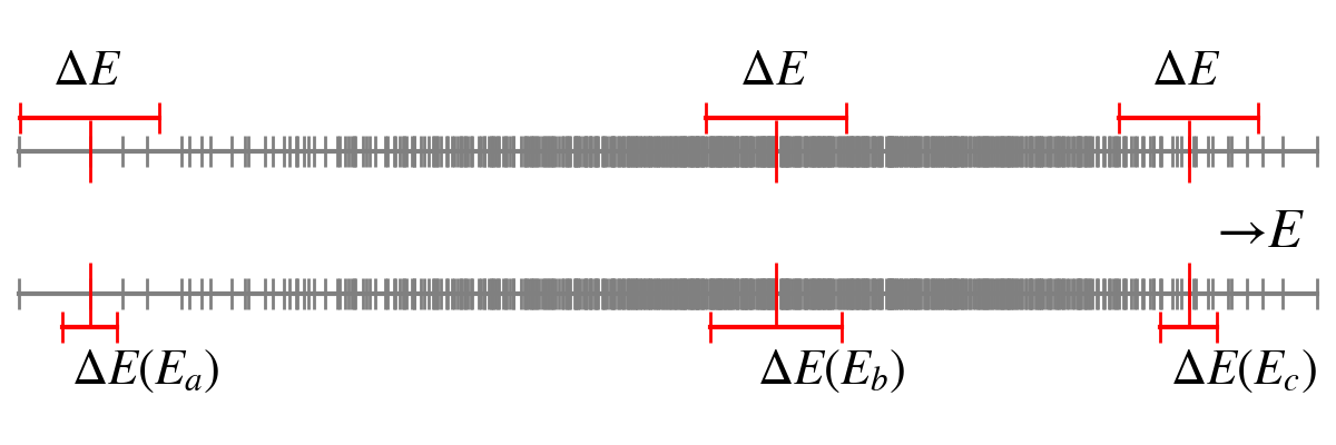
Figure 1: Illustration of two ways of choosing the energy window $\Delta E$ used to define the microcanonical entropy. The top figure shows the obvious choice: the width $\Delta E$ is the same at all energies. The lower schematic illustrates an energy-dependent width: $\Delta E(E)\propto\sqrt{T_{c}^{2}C_{c}}$, where the temperature $T_{c}$ is the canonical temperature corresponding to energy $E$ and $C_{c}$ is the heat capacity at $T=T_{c}$. The window is shown at three energy values $E_{a}$, $E_{b}$, and $E_{c}$, which are in the regions of low temperature, infinite temperature, and low negative temperature. Each vertical tick marks an eigenvalue.

First, we consider counting eigenstates in an arbitrarily chosen but constant (energy-independent) width window, as illustrated in Figure 1(top). This is the most obvious choice but turns out to be far from optimal — the resulting temperature deviates strongly at finite sizes from the canonical temperature.

Second, noting that the leading correction to the large-size limit can be made to disappear by choosing $\Delta E\propto\sqrt{T_{c}^{2}C_{c}}$ [62], we examine the result of using such an energy-dependent window width. (Here $C_{c}$ is the heat capacity.) Such an energy-dependent window is illustrated in Figure 1(bottom). We show that this choice works extremely well for the sizes of interest, modulo some caveats regarding the proportionality constant.

Finally, we can compute the microcanonical entropy using standard numerical estimation procedures for the d.o.s. via approximations to the integrated d.o.s. or cumulative spectral function. We first formulate the definition without reference to a specific energy window $\Delta E$ and show that this choice is sub-optimal. We analyze the reason for the strong finite-size mismatch in this case. Secondly, we show that using the energy-dependent $\Delta E\propto\sqrt{T_{c}^{2}C_{c}}$, designed to account for finite-size effects, results in excellent agreement between the temperatures even at the small sizes investigated, without any fine-tuning of proportionality constants.

This article is organized as follows. Section II recounts the definitions and saddle-point expressions that lead to the various choices for calculating the microcanonical entropy. We also provide details (II.3) of the quantum many-body systems that we use for numerical exploration — we provide results for multiple systems with different geometries, to ensure that the resulting conclusions are not artifacts of a particular lattice or Hamiltonian. In the next three sections, we describe the procedures for, and the results of, the four ways of calculating entropy. First, Section III describes counting eigenstates in a constant-width energy window $\Delta E$. Second, Section IV describes counting eigenstates in an energy-dependent window $\Delta E(E)$, designed to cancel out the explicit $\Delta E$-dependence of the resultant temperature, following/extending the suggestion of Ref. [62]. Third, Section V outlines using a smoothened cumulative d.o.s. $\Omega(E)$ to calculate the d.o.s. $g(E)$. We can then choose either to neglect $\Delta E$, which we explain leads to deviations, or make use of the derived energy dependent $\Delta E(E)$ designed to account for these deviations. Section VI provides concluding discussion and some context.

II Preliminaries

We first recall the standard definition of microcanonical entropy and highlight the roles of the density of states $g(E)$ and of the energy window $\Delta E$ (subsection II.1). We then recall (II.2) the saddle-point formulation often used to show the equivalence of microcanonical and canonical ensembles in the large-size limit [62], and extend beyond the leading order in order to analyze the effect of $\Delta E$ at finite sizes. Subsection II.3 describes the quantum systems to be used in subsequent sections to provide numerical examples.

II.1 Entropy, density of states, and the energy window

The microcanonical entropy $S(E)$ of a system at energy $E$ is [62, 57, 58, 59, 60, 61]

$$S(E)=k_{B}\ln\Gamma(E),$$ (3)

where $\Gamma(E)$ is the statistical weight, which is the number of microstates at energy $E$. For a quantum system, microstates are to be interpreted as eigenstates. For a quantum system with a discrete spectrum, counting the number of eigenstates is problematic because at any particular energy there is usually zero or one eigenstate, or perhaps a handful if there are degeneracies. Thus, $S(E)$ would be $=-\infty$ for all values of energy except at a countable number of discrete energy values. This issue is usually resolved [62, 59, 60] by taking $\Gamma(E)$ to be the number of eigenstates in an energy window $\Delta E$ around $E$, rather than the number of eigenstates exactly at energy $E$. Thus we define

$$\Gamma(E) =\int_{E-\Delta E/2}^{E+\Delta E/2}g(E^{\prime})dE^{\prime}$$

$$=\int_{E-\Delta E/2}^{E+\Delta E/2}\sum_{n}\delta(E^{\prime}-E_{n})dE^{\prime},$$ (4)

where the sum is understood to to include all the eigenvalues of the system Hamiltonian that lie in the window, i.e., all $E_{n}$ satisfying $E_{n}\in(E-\frac{\Delta E}{2},E+\frac{\Delta E}{2})$ . It is then common to approximate this integral [62, 64, 65, 66, 67] via

$$\Gamma(E)\approx\Delta Eg(E)=\Delta E\sum_{n}\delta(E-E_{n}).$$ (5)

Here, $g(E)$ is the density of states — the number of many-body eigenstates per unit energy interval. Although defined as a sum over delta functions, the density of states can be thought of as a smooth function of energy over energy scales much larger than the typical level spacing. In numerical work, this is often achieved by broadening the delta functions into Gaussians or Lorentzians of finite width [68, 69, 70, 24, 71, 72, 73, 74, 75]. Alternatively, we can define $\Omega(E)$ as the number of eigenstates with energy less than $E$, i.e., the integrated density of states. Fitting a smooth function to the staircase form of $\Omega(E)$, one can obtain a smooth density of states as the derivative; $g(E)=\Omega^{\prime}(E)$.

The entropy now depends on an energy window $\Delta E$, so we are thus faced with choosing an appropriate $\Delta E$. The purpose of introducing a finite energy width was to smooth out the discreteness of the energy spectrum, so $\Delta E$ should be large enough to include a large number of eigenstates. On the other hand, we want $\Delta E$ to be sufficiently small so that the density of states (regarded as a smooth function of energy) does not vary appreciably within the window, i.e., $\Delta E$ should be much smaller than the scale of the bandwidth of the system. Other than these general principles, we have the freedom to choose $\Delta E$, and in general, the entropy $S$ will depend on the choice.

As we will explain next (II.2), the sub-leading contributions to the entropy, which contain $\Delta E$, vanish in the large system size limit. So, for infinite systems, it will generally not matter what $\Delta E$ is, but the choice can drastically affect the entropy and resultant temperature for finite quantum systems. This paper aims to investigate and clarify the effect of this choice for finite systems whose Hilbert space sizes make them accessible to full numerical diagonalization.

II.2 Saddle point expressions

To understand the role of $\Delta E$, it is helpful to express the entropy as an integral over (complex) inverse temperature and perform saddle-point approximations [62, 56, 58], extending the order beyond what is necessary in the thermodynamic limit, to account for finite sizes.

Replacing the delta function in Eq. (5) with $\delta(x)=\int_{-\infty}^{\infty}(2\pi)^{-1}e^{i\beta x}d\beta$, and defining the free energy as $F(\beta)=-\beta^{-1}\ln(\sum_{n}e^{-\beta E_{n}})$, we can write the entropy as

$$e^{S/k_{B}}=\Gamma(E)=\Delta E\int_{-i\infty}^{i\infty}\frac{d\beta}{2\pi}e^{\beta(E-F(\beta))}.$$ (6)

To apply the saddle-point approximation, one first finds the critical point of the exponent $h(\beta)=\beta(E-F(\beta))$. The condition is

$$E-F(\beta)-\beta\frac{\partial F}{\partial\beta}=0\ ,$$ (7)

which is equivalent to Eq. (1) defining the canonical temperature. Thus the saddle point is at $\beta=\beta_{c}$, the canonical inverse temperature. The leading order saddle-point approximation is thus

$$\frac{S}{k_{B}}=\beta_{c}E-\beta_{c}F(\beta_{c})$$ (8)

with $\beta_{c}$ being the solution of Eq. (7) or Eq. (1). This matches the standard thermodynamic relation, and is consistent with the energy derivative of $S$ being the inverse temperature $\beta_{c}$.

To examine the effect of $\Delta E$, one needs to extend the calculation to the next order. One expands $h(\beta)$ as a Taylor series about $\beta_{c}$, up to second order, as the first order term is zero by definition. Introducing the heat capacity $C=\frac{\partial E}{\partial T}=-T\frac{\partial^{2}F}{\partial T^{2}}$, one obtains [62]

$$e^{S/k_{B}}\approx\frac{\Delta E}{2\pi}e^{\beta_{c}(E-F(\beta_{c}))}\int_{-\infty}^{\infty}dye^{-k_{B}T_{c}^{2}C_{c}y^{2}/2}.$$ (9)

Here, $T_{c}$ and $C_{c}$ are the values at the saddle point $\beta_{c}$. Evaluating the Gaussian integral, one obtains

$$\frac{S}{k_{B}}=\beta_{c}E-\beta_{c}F(\beta_{c})+\ln\Delta E-\ln\sqrt{2\pi k_{B}T_{c}^{2}C_{c}}.$$ (10)

Here $\beta_{c}$ is determined by the energy, and hence so are $T_{c}$ and $C_{c}$. The two leading terms are both extensive in system size. The first correction term $\ln\Delta E$ is sub-extensive as long as $\Delta E$ is not chosen to grow exponentially or faster with system size. The second correction term grows logarithmically with system size, as the heat capacity is extensive. However, as it appears in the argument of a logarithm, its dependence on $L$ disappears when differentiated with respect to $E$. This means that when differentiating Eq. (10) to obtain $\beta$, the contribution from the last term does not grow with $L$, not even logarithmically. Thus, at large enough sizes, the leading-order saddle-point approximation suffices, and the choice of energy window $\Delta E$ plays no role.

However, the two correction terms should be considered when calculating the entropy at finite sizes. From Eq. (10), we see that choosing $\Delta E$ to be an energy-independent constant (the most obvious choice, explored in Section III) would leave an energy-dependent correction term, causing deviations from the canonical temperature. We also see (as pointed out in Ref. [62] and explored below in Section IV) that the energy dependence of the correction terms could be canceled by a judicious choice of energy dependence for the width $\Delta E$.

II.3 Hamiltonians and numerics

To investigate the effect of different choices for defining the microcanonical entropy in finite systems, we use several spin-1/2 lattice systems consisting of $L$ spins, $N$ of which are up. The spins interact via XXZ interactions, which have a $U(1)$ symmetry conserving $N$. We check all results and show data for 1D, 2D, and fully-connected geometries, to demonstrate that our results are very general and not particular to any model. In the case of the 1D chain, we also include magnetic fields in the $z$ and $x$ directions; the latter break the $U(1)$ symmetry. The Hilbert space dimension is $D=\binom{L}{N}$ when $N$ is conserved and $D=2^{L}$ otherwise.

The system parameters are always chosen such that the level spacing statistics match that expected of chaotic quantum systems. This ensures there are no complications due to proximity to integrability or localization.

Staggered field XXZ chain: Starting with the open-boundary XXZ chain (anisotropic Heisenberg chain)

$$H_{H}=J\sum_{j=1}^{L-1}(S^{x}_{j}S^{x}_{j+1}+S^{y}_{j}S^{y}_{j+1})+\Delta\sum_{j=1}^{L-1}S^{z}_{j}S^{z}_{j+1}$$ (11)

we introduce magnetic fields in both the transverse ($x$) and longitudinal ($z$) directions. To remove symmetries in the model we stagger the two fields along the even and odd sites respectively, and in addition, we break the staggered pattern at the start of the chain by inserting $x$ and $z$ fields on the first and second sites respectively:

$$H_{S}=H_{H}+\sum_{j}h_{z}S^{z}_{2j+1}+\sum_{j}h_{x}S^{x}_{2j}+h_{x}S^{x}_{1}+h_{z}S^{z}_{2}.$$ (12)

Square Lattice: This model is a two-dimensional square lattice with open boundary conditions and XXZ interactions:

$$H_{\text{SQ}}=\sum_{\langle j,k\rangle}J_{jk}(S^{x}_{j}S^{x}_{k}+S^{y}_{j}S^{y}_{k})+\Delta_{jk}S^{z}_{j}S^{z}_{k}$$ (13)

where $\langle\rangle$ means that we restrict the summation to nearest-neighbor pairs. In order to remove any symmetries, we draw the values $J_{jk}$, $\Delta_{jk}$ from the uniform distributions $[0,2]$, $[0,1]$ respectively.

Fully connected Lattice: This model consists of a network of spins, where each spin $j$ is connected to every other spin $k$:

$$H_{\text{FC}}=\sum_{j}\sum_{k\neq j}J_{jk}(S^{x}_{j}S^{x}_{k}+S^{y}_{j}S^{y}_{k})+\Delta_{jk}S^{z}_{j}S^{z}_{k}$$ (14)

We draw the values $J_{jk}$, $\Delta_{jk}$ from the uniform distribution $[-0.4,0.4]$ and $[-0.1,0.1]$ respectively.

Units: For numerical work, we use $k_{B}=1$. We express energies in units of spin couplings. Thus, if the coupling $J$ (or $J_{jk}$) is set to 1, when we plot energy values, they are $E/J$; whereas if the couplings have other values, then the energy is to be thought of as the energy divided by a hypothetical coupling equal to $1$. In this way, the units of all energies, temperatures, and entropies presented in the figures are determined.

III Constant width window

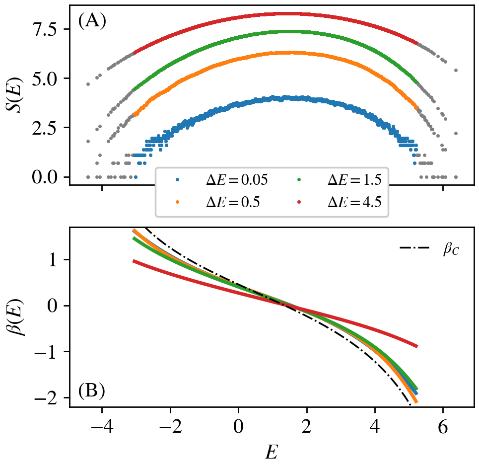
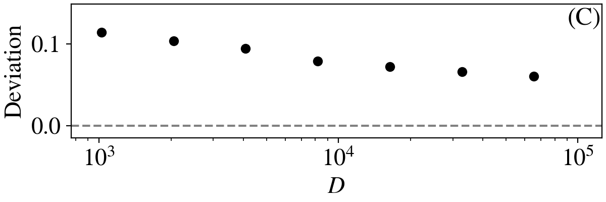
Figure 2: (A) Microcanonical entropy $S(E)$ calculated with constant (energy-independent) $\Delta E$. Evaluated only at the eigenenergies $E=E_{n}$. (B) Resultant inverse temperature $\beta(E)$ obtained as derivative of 6th-order polynomial fitted to $S(E)$ data. 25 eigenstates from both ends of the spectrum (shown in gray in (A)) were excluded from the fit. (A,B) $5\times$4 square XXZ lattice, Eq. (13), with $L=5\times 4$, $N=4$. (C): Root-mean-square (RMS) distance between $\beta(E)$ and the canonical temperature, versus Hilbert space dimension $D=2^{L}$, with $\Delta E=0.5$. Spin chain with $L$ spins, Eq. (12), $J=1$, $\Delta=0.95$, $h_{z}=h_{x}=0.5$. Units used in this and all subsequent figures are explained in subsection II.3.

We start by discussing the obvious choice for defining entropy — counting eigenstates in a constant energy-independent width $\Delta E$. Eq. (10) implies that an energy-independent $\Delta E$ acts as an energy-independent shift of the entropy, and hence does not affect the temperature. However, the last term in Eq. (10) is energy-dependent, hence the temperature will differ from the canonical temperature which corresponds to the leading (first two) terms. This deviation should vanish in the large-size limit, but the extent of this deviation for finite sizes is not a priori clear. We show below using explicit numerical examples that using an energy-independent width is a poor choice for the system sizes under study here (sizes accessible to exact diagonalization), as the resulting temperature deviates significantly from the canonical temperature.

Examples of entropy found by counting the number of eigenvalues within the window $[E-\Delta E/2,E+\Delta E/2]$, are shown in Figure 2(A) for an open-boundary square spin-$\frac{1}{2}$ lattice with random XXZ interactions. Here and in later figures, we plot one point for each eigenvalue, so that there is at least one eigenvalue in each window — the minimum value of entropy is $\ln 1=0$ and we thus avoid the possibility of obtaining entropy $\ln 0=-\infty$.

To calculate the temperature from the entropy, we fit a polynomial to the $S(E)$ points and then take the derivative of the polynomial; results are shown in Figure 2(B).

Increasing $\Delta E$ by a factor approximately increases the number of eigenvalues in each window by that factor, so that the $S(E)$ curve undergoes an approximately constant upward shift. This leaves the temperature $[S^{\prime}(E)]^{-1}$ approximately unchanged. Accordingly, for moderate $\Delta E$, the calculated $\beta(E)$ curves are robust to changes in $\Delta E$. For the largest $\Delta E(=4.5)$ shown, this argument does not work as the window is significant compared to the variation scale of the density of states $g(E)$, so that $g(E)$ cannot be considered constant within each window. This leads to a markedly different $\beta(E)$ curve for the very large $\Delta E$ case. This effect is not captured by the saddle-point analysis or Eq. (10).

Even for moderate $\Delta E$, the deviation from the canonical $\beta_{C}(E)$ curve is considerable. This shows that using a constant energy window width is not a feasible approach to defining entropy for finite quantum systems having Hilbert space dimensions $\sim{}O(10^{4})$. The results of Figure 2(B) provide a visual presentation of the extent of the discrepancy for such sizes. In Figure 2(C) we show the root-mean-square deviation of the inverse temperatures obtained with a constant $\Delta E$ from the canonical $\beta_{C}(E)$ values, as a function of Hilbert space dimension. (We show data for a spin chain, for which finite size scaling is numerically more convenient than for a square lattice.) The deviation decreases with increasing size, as expected, but very slowly.

A remark on the edges of the spectrum is in order. In the edge regions, as there are only a few eigenvalues in each window, the values of entropy are noticeably discrete, $\ln n$ where $n$ is a small integer. For a regime with such discrete behavior, statistical-mechanical considerations are not meaningful — we expect entropy to be a continuous function of energy. We therefore omit the edges from the polynomial fit to $S(E)$. In Figure 2 we have omitted 25 eigenstates from each edge of the spectrum. This is approximately the energy region for which $S(E)\lesssim\ln 10$ for the $\Delta E=0.5$ case. Later in the paper, the same criterion will be used to exclude the spectral edges.

IV Energy dependent window

We now describe counting eigenstates in an energy-dependent $\Delta E\propto\sqrt{T_{c}^{2}C_{c}}$.

IV.1 Rationale

In Eq. (10), the leading-order terms (first two terms) yield the canonical temperature upon differentiation by energy, but there are two correction terms, $\ln\Delta E$ and $-\ln\sqrt{2\pi{k_{B}}T_{c}C_{c}}$. Ref. [62] suggests choosing the two terms to be equal so that the corrections vanish and the canonical temperature is recovered.

We note, however, that the correction terms need not cancel exactly — they will not affect the temperature $[S^{\prime}(E)]^{-1}$ as long as they sum to an energy-dependent constant. Thus we could choose

$$\Delta E(E)\equiv\alpha^{-1}\sqrt{2\pi k_{B}T_{c}^{2}C_{c}}.$$ (15)

with $\alpha$ being some constant. The window $\Delta E$ is then energy-dependent because $T_{c}$ and $C_{c}$ are energy-dependent. The proposal of Ref. [62] corresponds to $\alpha=1$.

The energy-dependent $\Delta E$ can also be motivated by the physical idea that the energy window should be determined by the fluctuation of energy in the canonical ensemble, as suggested, e.g., in Refs. [64, 65]. It turns out [58] that the distribution in energy in the canonical ensemble has width $\propto\sqrt{T^{2}C}$. Thus, choosing the energy uncertainty as the energy window leads to the same prescription as Eq. (15).

Labeling the number of states in an energy-dependent energy window $\Delta E(E)$ as $\tilde{\Gamma}(E)$, the entropy is obtained as

$$\tilde{S}(E)=k_{B}\ln\left(\tilde{\Gamma}(E)\right).$$ (16)

Differentiation gives the corresponding inverse temperature $\tilde{\beta}$. In the following subsection we will describe doing this numerically, and discuss the results obtained.

We do not know of a principle guiding the choice of $\alpha$. We will show that, for the sizes of primary interest to us, $\alpha$ needs to be larger than $1$.

The reason is that for $\alpha=1$, the energy window $\Delta E(E)$ turns out to be too broad, exceeding the energy scale at which the density of states varies, leading to poor results similar to the large constant $\Delta E$ case in Figure 2. This is clear from Eq. (15); the right-hand side scales like $\sqrt{L}$ as $C_{c}$ is extensive, while the variance of the density of states typically scales linearly with $L$. Thus, for the system sizes under consideration here, $\sqrt{L}$ can not be considered negligible compared with $L$. For larger system sizes, the acceptable range of $\alpha$ broadens, compatible with our expectation that the choice of $\Delta E$ should be less important for larger sizes.

IV.2 Numerical calculation and results

In order to obtain $\Delta E(E)$ as defined in Eq. (15), we first need to calculate the heat capacity $C_{c}$ and the canonical temperature. We start by numerically computing the energy $E$ as a function of $\beta$ (or of $T$) via Eq. (1), using the numerically calculated eigenvalues of the Hamiltonian $H$. This leaves us with a (numerical approximation to a) smooth injective function $E(T)$. As usual, inverting this numerically provides the canonical temperature $T_{c}$ as a function of $E$. In addition, estimating the derivative of $E(T)$ provides us with the heat capacity $C=\partial E/\partial T$, which we evaluate at the canonical value $T_{c}$. Figure 3(A) shows an example of $C_{c}$ as a function of energy, calculated in this way. The function is non-monotonic, going to zero at both zero and infinite temperatures.

Figure 3: (A): Specific heat $C=\partial E/\partial T$. (B): $\Delta E(E)=\alpha^{-1}\sqrt{2\pi k_{B}T_{c}^{2}C_{c}}$, for $\alpha=5$, numerically computed. Dashed curve: 12-th order polynomial fit, used to avoid the spurious divergence. Data for $5\times$4 square XXZ lattice, Eq. (13), with $N=4$.

We can now calculate $\Delta E(E)$ via (15) for all energies. Figure 3(B) shows an example.

At the center of the spectrum, $T_{c}\to\infty$ and $C_{c}\to 0$, leading to a finite $\Delta E(E)\propto\sqrt{T_{c}^{2}C_{c}}$. Due to the numerical discreteness of computed $E$ and $T$ functions, the computed $\Delta E(E)$ acquires a spurious divergence at this point. This effect can be confined to a smaller energy region by using a finer grid of $T$ (or $E$) values. We avoid the effect by fitting a polynomial, excluding points within the direct vicinity of the discontinuity. An example is shown in Figure 3(B). The fitted polynomial is then used as $\Delta E(E)$.

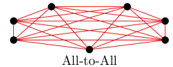
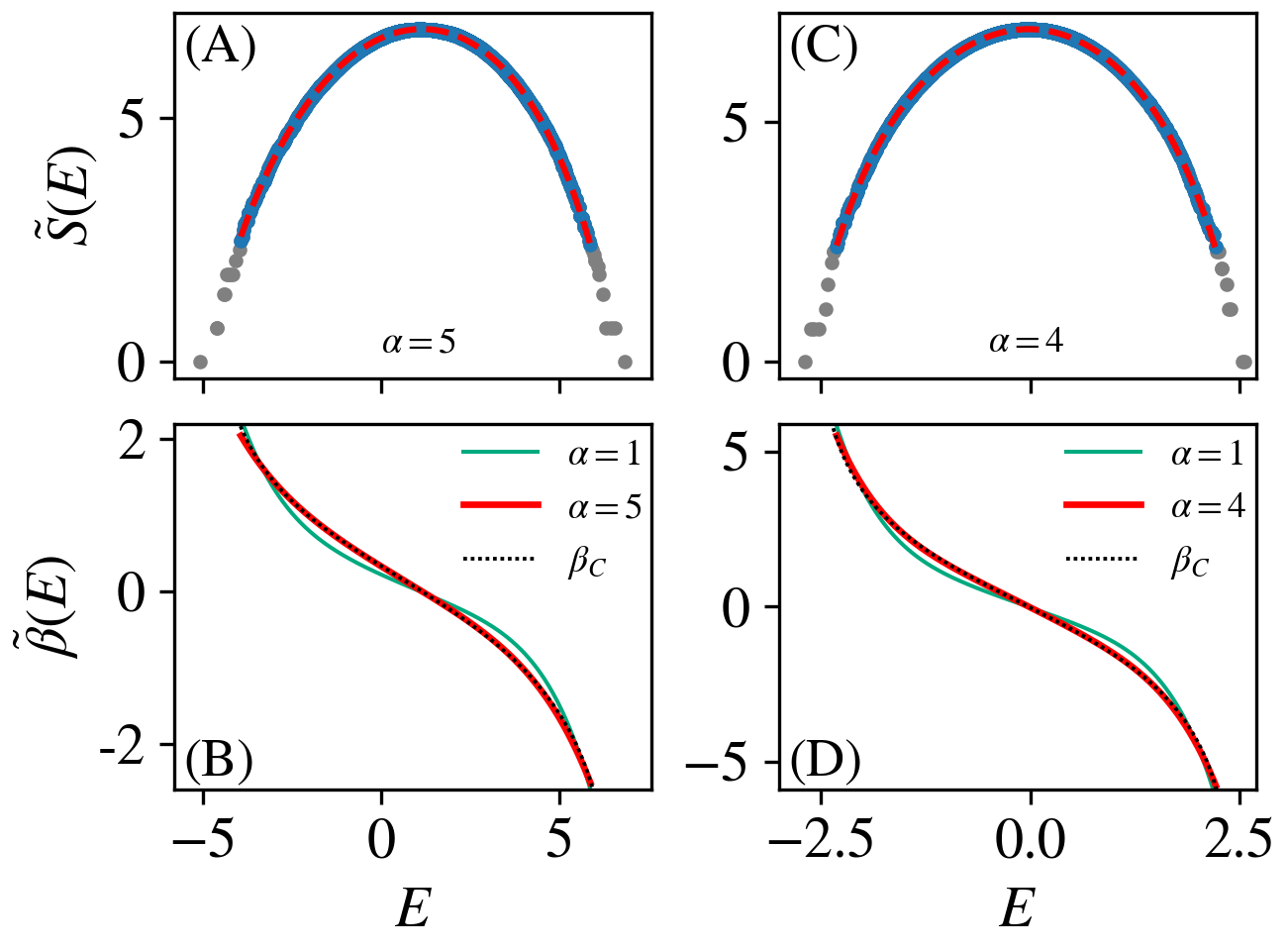
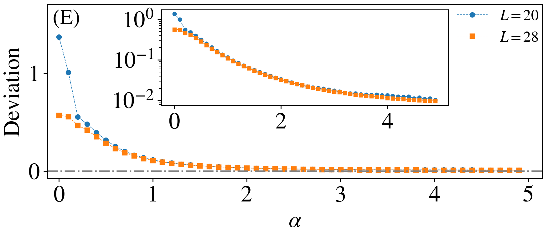
Figure 4: Using an energy-dependent window, Eq. (15). Left panels (A,B) and right panels (C,D) show data for two different systems. (A,C): Microcanonical entropy calculated with $\Delta E(E)=\alpha^{-1}\sqrt{2\pi k_{B}T_{c}^{2}C_{c}}$ along with 6th-order polynomial fit. Fit excludes gray points. (B,D) Resultant temperature $\tilde{\beta}(E)$, with two different values of $\alpha$ in each case, compared with canonical temperature $\beta_{C}(E)$. (A,B) Data for $5\times$4 square XXZ lattice, Eq. (13), with $N=4$. (C,D) Fully connected lattice, , Eq. (14), with $L=16$, $N=5$. (E) RMS distance between $\tilde{\beta}(E)$ and $\beta_{C}(E)$ plotted against $\alpha$ for two square lattices, Eq. (13), a $5\times 4$ lattice with $N=4$, and a $7\times 4$ lattice with $N=5$. Inset: logarithmic scale.

We are now equipped to compute the entropy using an energy dependent energy window, $\Delta E(E)=\alpha^{-1}\sqrt{2\pi k_{B}T_{c}^{2}C_{c}}$. In Figure 4(A,C), we show the numerically computed entropy $\tilde{S}$. The data shown is for a chaotic square lattice of spins-1/2’s with XXZ-like connections between nearest neighbor spins, and also for a fully connected lattice with XXZ-like connections between every pair of sites. We used $\alpha=5$ and $\alpha=4$ in the two cases.

As before, we numerically fit a polynomial to our entropy data, excluding values at the edge of the spectrum, and then take its derivative to obtain a temperature. The resultant inverse temperature $\tilde{\beta}$ are shown in Figures 4 (B,D). For $\alpha\sim 5$, the temperature matches the canonical temperature remarkably well.

We found that the procedure provides an excellent match between $\tilde{\beta}$ and $\beta_{c}$ when $\alpha$ is larger than some minimum value, as shown by the vanishing root-mean-square deviation in Figure 4(E). Beyond this minimal $\alpha$ the exact choice is somewhat arbitrary, as long as the window is not made ultra-small. Figure 4(E) shows that this minimal value (the value of $\alpha$ at which the deviation drops to zero) is smaller for larger systems. This is consistent with the expectation that the exact choice of the window $\Delta E$ is increasingly irrelevant as the system size is increased.

To summarize: this numerical analysis shows that using an energy-dependent window is a very successful strategy for defining entropy in a finite-size system. We observed good agreement between the resultant temperature and the canonical temperature for all systems we checked, including various 1D chaotic spin chains, and a handful of 2D lattices, including that presented in Figure 4.

V Using the integrated density of states

Here, we formulate the entropy in terms of the integrated d.o.s. $\Omega(E)$ and describe how to numerically obtain a smoothened approximation to the d.o.s. $g(E)=\Omega^{\prime}(E)$. First, we approximate the entropy by neglecting the $\Delta E$ contribution, and explain that this leads to finite-size deviations. Second, we use the smoothened $\Omega^{\prime}(E)$ with the energy-dependent $\Delta E(E)$ designed to account for the finite size deviations, and show that it leads to excellent agreement with the canonical temperature.

V.1 Formulation

An alternative to counting eigenstates in an explicit energy window is to use the expression for the entropy in terms of the (integrated) density of states:

$$S =k_{B}\ln\Gamma(E)=k_{B}\ln\bigg(g(E)\Delta E\bigg{missing})$$

$$=k_{B}\ln g(E)+k_{B}\ln\Delta E$$

$$=k_{B}\ln(\frac{\partial\Omega(E)}{\partial E})+k_{B}\ln\Delta E.$$ (17)

Here,

$$\Omega(E)=\sum_{n=1}^{D}\Theta(E-E_{n})$$ (18)

is the number of eigenstates $\ket{E_{n}}$ with energy less than $E$, i.e., the integrated d.o.s. or cumulative d.o.s., also known as the cumulative level density [76, 77, 78, 79, 80, 81, 82, 83, 84, 85, 86, 87] or the cumulative spectral function [88, 89, 13, 90, 91, 92, 93, 39, 94, 85, 95, 96].

Figure 5: Upper: Cumulative density of states $\Omega(E)$ (normalized by Hilbert space dimension), fitted by a polynomial $f(E)$ of degree 10. Inset: zoom. Lower: $\Omega^{\prime}(E)/D$ from derivative of fitted function, compared with histogram (distribution) of eigenvalues, $P(E_{n})$. Data for $7\times 4$ square XXZ lattice, Eq. (13), with $N=5$.

From the eigenvalue spectrum of the system Hamiltonian, computed numerically using exact diagonalization, the integrated d.o.s. $\Omega(E)$ can be obtained as a function of $E$. It is a series of steps with constant integer values between eigenvalues and a step to the next integer at every eigenvalue. In order to obtain a derivative of this non-smooth function, we will fit an analytic function to the computed $\Omega(E)$ data, and then simply take its derivative. Fitting an analytic function to $\Omega(E)$ is common practice in the unfolding procedure utilized for computing level spacing statistics [97, 98, 69, 99, 92, 39].

We found that using a function of the form

$$\frac{D}{2}\big{[}1+\tanh(f(E))\big{]}$$ (19)

works remarkably well to fit the numerical $\Omega(E)$ data, where $f(E)$ is some polynomial in $E$. If $f(E)$ is a monotonically increasing polynomial, then the form of the function automatically imposes the correct low-energy and high-energy behavior of the smoothened $\Omega(E)$. This functional form was inspired by its use in [93] to unfold a many-body spectrum. Once the fitting function $f(E)$ is determined, the density of states is obtained as the derivative:

$$g(E)=\Omega^{\prime}(E)=\frac{D}{2}\sech^{2}(f(E))f^{\prime}(E)$$ (20)

An example of numerically calculated $\Omega(E)$ and the fitted function are shown in Figure 5 (top). The resulting derivative $\Omega^{\prime}(E)$ is compared with the normalized histogram of eigenvalues (bottom). In both panels, we normalize the functions by $D$, so that the function itself is plotted between $0$ and $1$, and its derivative can be directly compared with the normalized eigenvalue distribution $P(E_{n})$. With $\Omega^{\prime}(E)$ in hand, we are now equipped to compute the entropy and resultant temperature. In the following subsections we present two ways to do so.

V.2 Using the integrated D.O.S. while avoiding $\Delta E$

The density of states increases exponentially with the system size; hence the first term in Eq. (V.1) is extensive. On the other hand, $\ln\Delta E$ is presumably either constant or at most weakly increasing with system size. Thus, at sufficiently large system sizes the second term can be neglected so that the first term approximates the entropy:

$$S\approx S_{\Omega}=k_{B}\ln g(E)=k_{B}\ln(\frac{\partial\Omega(E)}{\partial E}).$$ (21)

One can thus use a continuous approximation for $\Omega(E)$ to define a continuous $S_{\Omega}(E)$, without choosing an explicit energy window $\Delta E$.

$S_{\Omega}$ is the logarithm of $g(E)=\Omega^{\prime}(E)$, and $\beta_{\Omega}$ is thus the derivative of this. For the analytical approximation to $\Omega^{\prime}(E)$, Eq. (20), one obtains

$$\beta_{\Omega}(E)=\frac{f^{\prime\prime}(E)}{f^{\prime}(E)}-2f^{\prime}(E)\cdot\tanh(f(E)).$$ (22)

Examples of the computed entropy $S_{\Omega}$ are shown in Figure 6(A,C). The numerical results shown are for a 1D spin chain, and a square lattice, both with nearest neighbor XXZ-like connections and open boundary conditions. The resultant inverse temperatures $\beta_{\Omega}$ are shown in panels (B,D). While $\beta_{\Omega}$ has the correct overall form, the deviations from the canonical curves are clearly visible.

The extent of the deviation is shown quantitatively in Figure 6(E) by plotting the root-mean-square (RMS) distance between the canonical and resultant temperature, versus Hilbert space dimension $D$, for an $L$-site spin chain ($D=2^{L}$). The deviation decreases very slowly — it would take very large system sizes for the two temperatures to be considered ‘close’.

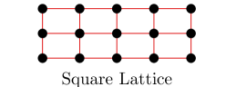
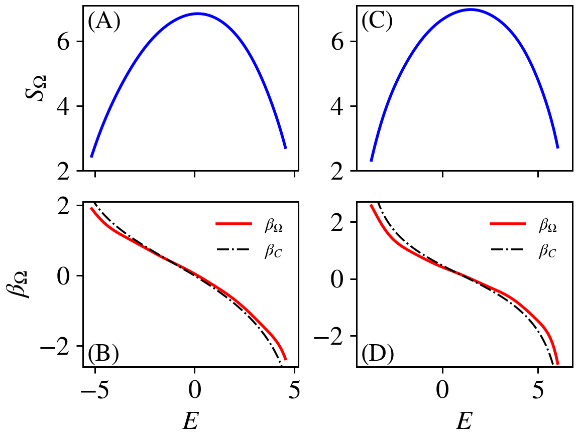
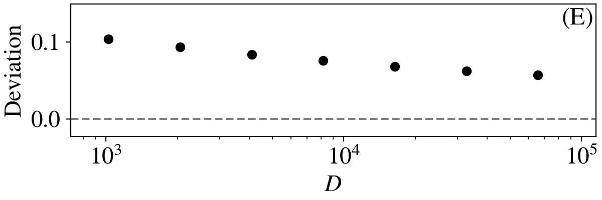
Figure 6: Entropy and temperature using a continuous approximation to the cumulative density of states. (A,C) $S_{\Omega}=\ln\Omega^{\prime}(E)$. (B,D) Resultant inverse temperature $\beta_{\Omega}=\partial_{E}S_{\Omega}$ compared with the canonical temperature $\beta_{C}$. (A,B) Staggered field XXZ chain, Eq. (12), with $L=12$, $J=1$, $\Delta=0.95$, $h_{z}=h_{x}=0.5$. (C,D) $5\times 4$ square XXZ lattice, Eq. (13), with $N=4$. (E) RMS distance between $\beta_{\Omega}(E)$ and $\beta_{C}(E)$, versus $D$ $(2^{L})$, for the spin chain, Eq. (12), with the same parameters as in (A,B) and variable $L$.

We now discuss two ways of understanding this finite size deviation. First, using Eq. (21) for the entropy means omitting the $\ln\Delta E$ term from the definition, Eq. (V.1), which can be written as

$$S=S_{\Omega}+k_{B}\ln\Delta E.$$ (23)

Since we avoided making an explicit choice for $\Delta E$, it is not obvious what the effect of dropping the second term is, but we can analyze different cases:

• If we consider $\Delta E$ to be energy-independent, then $S_{\Omega}$ will lead to the same temperature as obtained from the full microcanonical entropy $S$. However, we know from Section III that $S$ obtained using an energy-independent $\Delta E$ leads to considerable finite-size deviations in the temperature.

• On the other hand, if $\Delta E$ were to be energy-dependent, e.g., if it were designed to cancel the sub-leading deviations from the canonical ensemble as in Section IV, then $S_{\Omega}^{\prime}(E)$ will differ from $S^{\prime}(E)$, and we would again get finite-size deviations.

Thus, it appears that $S_{\Omega}^{\prime}(E)$ can be expected to deviate from $\beta_{c}$ in either case.

Second, we note that Eq. (21) applies the logarithm to a dimensionful quantity, which strictly speaking is not allowed. For consistency, one needs to multiply the argument of the logarithm in Eq. (21) by a quantity having the dimensions of energy; let us call this quantity $\epsilon$. Then Eq. (21) should really have the form

$$S_{\Omega}=\ln\left[g(E)\epsilon\right]=\ln\left[\Omega^{\prime}(E)\epsilon\right].$$ (24)

One can then carry out the same saddle point approximation as previously performed (subsection II.2) with the original definition of $S$, leading to

$$\frac{S_{\Omega}}{k_{B}}\approx\beta_{c}E-\beta_{c}F(\beta_{c}))+\ln\epsilon-\ln\sqrt{2\pi k_{B}T_{c}^{2}C_{c}}.$$ (25)

Unless $\epsilon$ is carefully chosen (as we did for $\Delta E$ in Section IV), the last term will lead to finite-size deviations. The procedure in this section avoids specifying $\Delta E$ and ignores the need for the quantity $\epsilon$. Thus, one would expect deviations due to the $-\ln\sqrt{T_{c}^{2}C_{c}}$ term, essentially of the same type as that encountered in III when using an explicit energy-independent value of $\Delta E$.

V.3 Using the integrated D.O.S. with an energy dependent window

Now, rather than neglect $\Delta E$ in Eq. (V.1), we retain the term, i.e., we consider the entropy in terms of the integrated d.o.s. as

$$S(E)=k_{B}\ln(g(E)\Delta E)=k_{B}\ln(\frac{\partial\Omega(E)}{\partial E}\Delta E).$$ (26)

We have a smooth approximation to $\Omega^{\prime}(E)$, and as proposed in Section IV, we could choose an energy-dependent $\Delta E(E)\propto\sqrt{T_{c}^{2}C_{c}}$ to account for the finite size deviations. Here, the constants of proportionality will only result in a shift in entropy, as we are not counting eigenstates in an energy window of width $\Delta E(E)$ around $E$. In that case, we had to choose a constant $\alpha$, such that the window width was not comparable to the bandwidth of the spectrum.

Here, rather than count the number of eigenstates, we use the derivative of our smoothed approximation to the integrated d.o.s. to compute $g(E)$. The proportionality constants in this case are arbitrary, thus our entropy can now be written as

$$S_{\Omega}(E)=\ln\left[\Omega^{\prime}(E)\sqrt{T_{c}^{2}C_{c}}\right].$$ (27)

Again, we use $\Omega^{\prime}(E)=\frac{D}{2}\sech^{2}(f(E))f^{\prime}(E)$. Determining the canonical temperature $T_{c}$ and heat capacity $C_{c}$ numerically has been previously discussed (subsection IV.2). Thus we can calculate the entropy (27) and by fitting a polynomial to the resulting curve, we can derive the inverse temperature.

Examples of the computed entropy $S_{\Omega}(E)$ are shown in Figure 7(A,C). The numerical results shown are for a 1D spin chain and a square lattice, both with nearest neighbor XXZ-like connections and open boundary conditions. The resultant inverse temperatures $\beta_{\Omega}(E)$ are shown in panels (B,D). We see that $\beta_{\Omega}(E)$ aligns very well with the canonical temperature $\beta_{c}$. A pleasing aspect of this method is that it requires no fine-tuning of constants, as they only result in a shift of entropy.

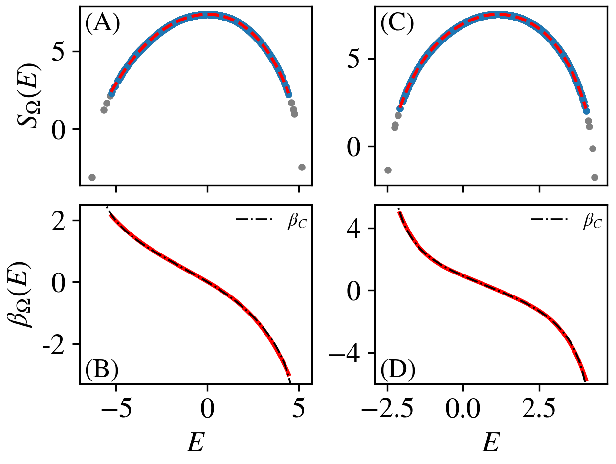
Figure 7: Entropy and temperature using a continuous approximation to the cumulative density of states and an energy dependent $\Delta E(E)=\sqrt{T_{c}^{2}C_{c}}$. (A,C) $S_{\Omega}(E)=\ln(\Omega^{\prime}(E)\Delta E(E))$. (B,D) Resultant inverse temperature $\beta_{\Omega}(E)=\partial_{E}S_{\Omega}(E)$ compared with the canonical temperature $\beta_{C}$. (A,B) Staggered field XXZ chain, Eq. (12), with $L=12$, $J=1$, $\Delta=0.95$, $h_{z}=h_{x}=0.5$. (C,D) $5\times 4$ square XXZ lattice, Eq. (13), with $N=4$.

VI Concluding Discussion & Context

The equivalence of microcanonical and canonical ensembles emerges in the infinite-size limit. Since statistical mechanics in isolated systems is being intensively discussed through finite-size examples obtained by numerical diagonalization, it is important to understand deviations from ensemble equivalence in systems of such sizes. In this work, we contribute to this question by investigating and comparing various ways of computing the microcanonical entropy, and then comparing the resultant temperatures (via Eq. (2)) to the canonical temperature (Eq. (1)).

The microcanonical entropy $S(E)$ is defined as in Eqs. (3) and (5). Inspired by the discussion of Ref. [62], we explored four ways of calculating $S(E)$ numerically: in terms of a constant-width energy window (Section III), using an energy-dependent window with the energy-dependence designed to cancel sub-leading terms (Section IV), and using the integrated density of states, first with an approximation that avoids the energy window altogether, and alternatively, in combination with an energy-dependent window (Section V).

We have demonstrated that counting eigenstates using the energy-dependent window, $\Delta E(E)=\alpha^{-1}\sqrt{2\pi k_{B}T_{c}^{2}C_{c}}$, works extremely well for the sizes under consideration. The use of this energy-dependent window was suggested by Ref. [62] with $\alpha=1$, designed to exactly cancel the sub-leading terms in Eq. (10). We have shown (Figure 4) that, for the sizes under question, a larger $\alpha$ is required, because for $\alpha=1$ the windows exceed the energy scale of variation of the density of states. A consequence of this result is that, since we have no further criterion for fixing $\alpha$, the microcanonical entropy is only defined up to an arbitrary additive constant. The constant is sub-extensive (and thus unimportant in the infinite-size limit), and an additive constant does not affect the temperature. In fact, a pleasing aspect of the suggestion of Ref. [62] was a reasonable criterion for defining entropy without such an arbitrary constant. For the size ranges under consideration in this work, the $\alpha=1$ prescription is not usable, so we are forced to accept an arbitrary shift.

However, using the entropy $S_{\Omega}(E)$ in Section V.3, combining the use of an energy-dependent $\Delta E(E)$ with an approximation to the d.o.s. constructed from the integrated d.o.s. $\Omega$, we observed excellent agreement between the resulting temperature and the canonical temperature. Here, the constants in $\Delta E(E)$ do not affect the resulting temperature, as they simply shift the entropy; this method is thus free from any fine-tuning of constants.

The other two procedures (counting eigenstates in an energy-independent $\Delta E$ and $S\approx S_{\Omega}$) both lead to very noticeable finite-size deviations. The deviations in the constant-$\Delta E$ case are expected from the sub-leading corrections. For the procedure in Section V using $S\approx k_{B}\ln(\Omega^{\prime}(E))$, we have argued that the deviations are essentially of the same type as that in the constant-$\Delta E$ case.

Numerical calculations of microcanonical entropy and/or temperature have appeared in the recent literature [65, 95, 66, 67]. Refs. [95, 67] have used the $S\approx S_{\Omega}$ approximation. The resulting temperature shown in Ref. [95] (Figure 4) appears to have similar deviations from the canonical temperature as we have presented and analyzed in Section V. The density of states is approximated in Ref. [95] via a polynomial fit to the cumulative spectral function and in Ref. [67] via the kernel polynomial method [100, 101]. In Ref. [65], the microcanonical entropy has been calculated with $\Delta E$ “determined by the energy uncertainty” — this is presumably equivalent to the energy-dependent window we explored in Section IV.

For finite quantum systems, the entanglement entropy of a subsystem is often discussed as representing the thermal entropy [102, 103, 36, 54, 55]. The reason is that, in a chaotic (thermalizing) quantum system, it is expected that the reduced density matrix of subsystems smaller than half the system should resemble thermal density matrices [104, 105, 53, 35, 36, 55, 106]. It is amusing to note that the entanglement entropy is obtained from eigenstates, whereas the entropies and temperatures studied in this work are derived from eigenenergies. Ref. [36] describes the finite-size behavior of the deviation of the entanglement entropy from the canonical entropy for a particular spin chain. The behavior of the temperature derived using Eq. (2) from the entanglement entropy (interpreted as the entropy) would be interesting to examine in future work.

It has been argued that entropy for finite-size systems should be defined as $S\sim\ln\Omega(E)$ [107, 108, 109, 110, 111, 112], instead of the more common $S\sim\ln\Omega^{\prime}(E)$ examined here. This approach avoids the appearance of negative temperatures even in systems with finite Hilbert space dimension. It may be interesting to ask how the deviations from ensemble equivalence behave under this alternate definition.

References

- Deutsch [1991] J. M. Deutsch, Quantum statistical mechanics in a closed system, Phys. Rev. A 43, 2046 (1991).
- Srednicki [1994] M. Srednicki, Chaos and quantum thermalization, Phys. Rev. E 50, 888 (1994).
- Srednicki [1996] M. Srednicki, Thermal fluctuations in quantized chaotic systems, Journal of Physics A: Mathematical and General 29, L75 (1996).
- Srednicki [1999] M. Srednicki, The approach to thermal equilibrium in quantized chaotic systems, Journal of Physics A: Mathematical and General 32, 1163 (1999).
- Rigol et al. [2008] M. Rigol, V. Dunjko, and M. Olshanii, Thermalization and its mechanism for generic isolated quantum systems, Nature 452, 854 (2008).
- D’Alessio et al. [2016] L. D’Alessio, Y. Kafri, A. Polkovnikov, and M. Rigol, From quantum chaos and eigenstate thermalization to statistical mechanics and thermodynamics, Advances in Physics 65, 239 (2016).
- Reimann [2015] P. Reimann, Eigenstate thermalization: Deutsch’s approach and beyond, New Journal of Physics 17, 055025 (2015).
- Deutsch [2018] J. M. Deutsch, Eigenstate thermalization hypothesis, Reports on Progress in Physics 81, 082001 (2018).
- Mori et al. [2018] T. Mori, T. N. Ikeda, E. Kaminishi, and M. Ueda, Thermalization and prethermalization in isolated quantum systems: a theoretical overview, Journal of Physics B: Atomic, Molecular and Optical Physics 51, 112001 (2018).
- Rigol [2009a] M. Rigol, Quantum quenches and thermalization in one-dimensional fermionic systems, Phys. Rev. A 80, 053607 (2009a).
- Rigol [2009b] M. Rigol, Breakdown of thermalization in finite one-dimensional systems, Phys. Rev. Lett. 103, 100403 (2009b).
- Biroli et al. [2010] G. Biroli, C. Kollath, and A. M. Läuchli, Effect of rare fluctuations on the thermalization of isolated quantum systems, Phys. Rev. Lett. 105, 250401 (2010).
- Santos and Rigol [2010a] L. F. Santos and M. Rigol, Onset of quantum chaos in one-dimensional bosonic and fermionic systems and its relation to thermalization, Phys. Rev. E 81, 036206 (2010a).
- Santos and Rigol [2010b] L. F. Santos and M. Rigol, Localization and the effects of symmetries in the thermalization properties of one-dimensional quantum systems, Phys. Rev. E 82, 031130 (2010b).
- Rigol and Santos [2010] M. Rigol and L. F. Santos, Quantum chaos and thermalization in gapped systems, Phys. Rev. A 82, 011604 (2010).
- Roux [2010] G. Roux, Finite-size effects in global quantum quenches: Examples from free bosons in an harmonic trap and the one-dimensional Bose-Hubbard model, Phys. Rev. A 81, 053604 (2010).
- Neuenhahn and Marquardt [2012] C. Neuenhahn and F. Marquardt, Thermalization of interacting fermions and delocalization in Fock space, Phys. Rev. E 85, 060101 (2012).
- Rigol and Srednicki [2012] M. Rigol and M. Srednicki, Alternatives to eigenstate thermalization, Phys. Rev. Lett. 108, 110601 (2012).
- Santos et al. [2012] L. F. Santos, A. Polkovnikov, and M. Rigol, Weak and strong typicality in quantum systems, Phys. Rev. E 86, 010102 (2012).
- Genway et al. [2012] S. Genway, A. F. Ho, and D. K. K. Lee, Thermalization of local observables in small hubbard lattices, Phys. Rev. A 86, 023609 (2012).
- Steinigeweg et al. [2013] R. Steinigeweg, J. Herbrych, and P. Prelovšek, Eigenstate thermalization within isolated spin-chain systems, Phys. Rev. E 87, 012118 (2013).
- Kim et al. [2014] H. Kim, T. N. Ikeda, and D. A. Huse, Testing whether all eigenstates obey the eigenstate thermalization hypothesis, Phys. Rev. E 90, 052105 (2014).
- Beugeling et al. [2014] W. Beugeling, R. Moessner, and M. Haque, Finite-size scaling of eigenstate thermalization, Phys. Rev. E 89, 042112 (2014).
- Sorg et al. [2014] S. Sorg, L. Vidmar, L. Pollet, and F. Heidrich-Meisner, Relaxation and thermalization in the one-dimensional Bose-Hubbard model: A case study for the interaction quantum quench from the atomic limit, Phys. Rev. A 90, 033606 (2014).
- Steinigeweg et al. [2014] R. Steinigeweg, A. Khodja, H. Niemeyer, C. Gogolin, and J. Gemmer, Pushing the limits of the eigenstate thermalization hypothesis towards mesoscopic quantum systems, Phys. Rev. Lett. 112, 130403 (2014).
- Fratus and Srednicki [2015] K. R. Fratus and M. Srednicki, Eigenstate thermalization in systems with spontaneously broken symmetry, Phys. Rev. E 92, 040103 (2015).
- Beugeling et al. [2015] W. Beugeling, R. Moessner, and M. Haque, Off-diagonal matrix elements of local operators in many-body quantum systems, Phys. Rev. E 91, 012144 (2015).
- Nandkishore and Huse [2015] R. Nandkishore and D. A. Huse, Many-body localization and thermalization in quantum statistical mechanics, Annual Review of Condensed Matter Physics 6, 15 (2015).
- Johri et al. [2015] S. Johri, R. Nandkishore, and R. N. Bhatt, Many-body localization in imperfectly isolated quantum systems, Phys. Rev. Lett. 114, 117401 (2015).
- Luck [2016] J. M. Luck, An investigation of equilibration in small quantum systems: the example of a particle in a 1d random potential, Journal of Physics A: Mathematical and Theoretical 49, 115303 (2016).
- Mondaini et al. [2016] R. Mondaini, K. R. Fratus, M. Srednicki, and M. Rigol, Eigenstate thermalization in the two-dimensional transverse field ising model, Phys. Rev. E 93, 032104 (2016).
- Chandran et al. [2016] A. Chandran, M. D. Schulz, and F. J. Burnell, The eigenstate thermalization hypothesis in constrained hilbert spaces: A case study in non-abelian anyon chains, Phys. Rev. B 94, 235122 (2016).
- Luitz and Bar Lev [2016] D. J. Luitz and Y. Bar Lev, Anomalous thermalization in ergodic systems, Phys. Rev. Lett. 117, 170404 (2016).
- Mondaini and Rigol [2017] R. Mondaini and M. Rigol, Eigenstate thermalization in the two-dimensional transverse field ising model. ii. off-diagonal matrix elements of observables, Phys. Rev. E 96, 012157 (2017).
- Dymarsky et al. [2018] A. Dymarsky, N. Lashkari, and H. Liu, Subsystem eigenstate thermalization hypothesis, Phys. Rev. E 97, 012140 (2018).
- Garrison and Grover [2018] J. R. Garrison and T. Grover, Does a single eigenstate encode the full Hamiltonian?, Phys. Rev. X 8, 021026 (2018).
- Yoshizawa et al. [2018] T. Yoshizawa, E. Iyoda, and T. Sagawa, Numerical large deviation analysis of the eigenstate thermalization hypothesis, Phys. Rev. Lett. 120, 200604 (2018).
- Khaymovich et al. [2019] I. M. Khaymovich, M. Haque, and P. A. McClarty, Eigenstate thermalization, random matrix theory, and behemoths, Phys. Rev. Lett. 122, 070601 (2019).
- Jansen et al. [2019] D. Jansen, J. Stolpp, L. Vidmar, and F. Heidrich-Meisner, Eigenstate thermalization and quantum chaos in the holstein polaron model, Phys. Rev. B 99, 155130 (2019).
- Mierzejewski and Vidmar [2020] M. Mierzejewski and L. Vidmar, Quantitative impact of integrals of motion on the eigenstate thermalization hypothesis, Phys. Rev. Lett. 124, 040603 (2020).
- Brenes et al. [2020a] M. Brenes, S. Pappalardi, J. Goold, and A. Silva, Multipartite entanglement structure in the eigenstate thermalization hypothesis, Phys. Rev. Lett. 124, 040605 (2020a).
- Santos et al. [2020] L. F. Santos, F. Pérez-Bernal, and E. J. Torres-Herrera, Speck of chaos, Phys. Rev. Research 2, 043034 (2020).
- LeBlond and Rigol [2020] T. LeBlond and M. Rigol, Eigenstate thermalization for observables that break hamiltonian symmetries and its counterpart in interacting integrable systems, Phys. Rev. E 102, 062113 (2020).
- Brenes et al. [2020b] M. Brenes, T. LeBlond, J. Goold, and M. Rigol, Eigenstate thermalization in a locally perturbed integrable system, Phys. Rev. Lett. 125, 070605 (2020b).
- Noh [2021] J. D. Noh, Eigenstate thermalization hypothesis and eigenstate-to-eigenstate fluctuations, Phys. Rev. E 103, 012129 (2021).
- Sugimoto et al. [2021] S. Sugimoto, R. Hamazaki, and M. Ueda, Test of the eigenstate thermalization hypothesis based on local random matrix theory, Phys. Rev. Lett. 126, 120602 (2021).
- Schönle et al. [2021] C. Schönle, D. Jansen, F. Heidrich-Meisner, and L. Vidmar, Eigenstate thermalization hypothesis through the lens of autocorrelation functions, Phys. Rev. B 103, 235137 (2021).
- Nakerst and Haque [2021] G. Nakerst and M. Haque, Eigenstate thermalization scaling in approaching the classical limit, Phys. Rev. E 103, 042109 (2021).
- Wang et al. [2022] J. Wang, M. H. Lamann, J. Richter, R. Steinigeweg, A. Dymarsky, and J. Gemmer, Eigenstate thermalization hypothesis and its deviations from random-matrix theory beyond the thermalization time, Phys. Rev. Lett. 128, 180601 (2022).
- Sugimoto et al. [2022] S. Sugimoto, R. Hamazaki, and M. Ueda, Eigenstate thermalization in long-range interacting systems, Phys. Rev. Lett. 129, 030602 (2022).
- Khatami et al. [2013] E. Khatami, G. Pupillo, M. Srednicki, and M. Rigol, Fluctuation-dissipation theorem in an isolated system of quantum dipolar bosons after a quench, Phys. Rev. Lett. 111, 050403 (2013).
- Essler and Fagotti [2016] F. H. L. Essler and M. Fagotti, Quench dynamics and relaxation in isolated integrable quantum spin chains, Journal of Statistical Mechanics: Theory and Experiment 2016, 064002 (2016).
- Kaufman et al. [2016] A. M. Kaufman, M. E. Tai, A. Lukin, M. Rispoli, R. Schittko, P. M. Preiss, and M. Greiner, Quantum thermalization through entanglement in an isolated many-body system, Science 353, 794 (2016).
- Lu and Grover [2019] T.-C. Lu and T. Grover, Renyi entropy of chaotic eigenstates, Phys. Rev. E 99, 032111 (2019).
- Seki and Yunoki [2020] K. Seki and S. Yunoki, Emergence of a thermal equilibrium in a subsystem of a pure ground state by quantum entanglement, Phys. Rev. Research 2, 043087 (2020).
- Reif [1965] F. Reif, Fundamentals of statistical and thermal physics (New York, McGraw-Hill, 1965).
- Reichl [1998] L. E. Reichl, A Modern Course in Statistical Physics (John Wiley & Sons, 1998).
- Huang [1987] K. Huang, Statistical Mechanics (John Wiley & Sons, 1987).
- Pathria [1996] R. K. Pathria, Statistical Mechanics (Butterworth-Heinemann, Oxford, 1996).
- Landau and Lifshitz [1969] L. D. Landau and E. M. Lifshitz, Statistical Physics (Pergamon, Oxford, 1969).
- Kardar [2007] M. Kardar, Statistical Physics of Particles (Cambridge University Press, 2007).
- Gurarie [2007] V. Gurarie, The equivalence between the canonical and microcanonical ensembles when applied to large systems, American Journal of Physics 75, 747 (2007).
- Note [1] It is also common to use the window . We choose to work with the window . This choice presumably does not have significant effects.
- Polkovnikov [2011] A. Polkovnikov, Microscopic diagonal entropy and its connection to basic thermodynamic relations, Annals of Physics 326, 486 (2011).
- Santos et al. [2011] L. F. Santos, A. Polkovnikov, and M. Rigol, Entropy of isolated quantum systems after a quench, Phys. Rev. Lett. 107, 040601 (2011).
- Russomanno et al. [2021] A. Russomanno, M. Fava, and M. Heyl, Quantum chaos and ensemble inequivalence of quantum long-range Ising chains, Phys. Rev. B 104, 094309 (2021).
- Mitchison et al. [2022] M. T. Mitchison, A. Purkayastha, M. Brenes, A. Silva, and J. Goold, Taking the temperature of a pure quantum state, Phys. Rev. A 105, L030201 (2022).
- Bruus and Angl‘es d’Auriac [1997] H. Bruus and J.-C. Angl‘es d’Auriac, Energy level statistics of the two-dimensional hubbard model at low filling, Phys. Rev. B 55, 9142 (1997).
- Gómez et al. [2002] J. M. G. Gómez, R. A. Molina, A. Relaño, and J. Retamosa, Misleading signatures of quantum chaos, Phys. Rev. E 66, 036209 (2002).
- Wang et al. [2010] C.-C. J. Wang, R. A. Duine, and A. H. MacDonald, Quantum vortex dynamics in two-dimensional neutral superfluids, Phys. Rev. A 81, 013609 (2010).
- Shchadilova et al. [2014] Y. E. Shchadilova, P. Ribeiro, and M. Haque, Quantum quenches and work distributions in ultralow-density systems, Phys. Rev. Lett. 112, 070601 (2014).
- Steinke et al. [2017] C. Steinke, D. Mourad, M. Rösner, M. Lorke, C. Gies, F. Jahnke, G. Czycholl, and T. O. Wehling, Noninvasive control of excitons in two-dimensional materials, Phys. Rev. B 96, 045431 (2017).
- Pixley et al. [2017] J. H. Pixley, Y.-Z. Chou, P. Goswami, D. A. Huse, R. Nandkishore, L. Radzihovsky, and S. Das Sarma, Single-particle excitations in disordered weyl fluids, Phys. Rev. B 95, 235101 (2017).
- Liu and Lu [2022] T. Liu and H.-Z. Lu, Analytic solution to pseudo-landau levels in strongly bent graphene nanoribbons, Phys. Rev. Research 4, 023137 (2022).
- Xiong et al. [2022] F. Xiong, C. Honerkamp, D. M. Kennes, and T. Nag, Understanding the three-dimensional quantum hall effect in generic multi-weyl semimetals, Phys. Rev. B 106, 045424 (2022).
- Gräf et al. [1992] H.-D. Gräf, H. L. Harney, H. Lengeler, C. H. Lewenkopf, C. Rangacharyulu, A. Richter, P. Schardt, and H. A. Weidenmüller, Distribution of eigenmodes in a superconducting stadium billiard with chaotic dynamics, Phys. Rev. Lett. 69, 1296 (1992).
- Relaño et al. [2004] A. Relaño, J. Dukelsky, J. M. G. Gómez, and J. Retamosa, Stringent numerical test of the poisson distribution for finite quantum integrable hamiltonians, Phys. Rev. E 70, 026208 (2004).
- Le et al. [2005] A.-T. Le, T. Morishita, X.-M. Tong, and C. D. Lin, Signature of chaos in high-lying doubly excited states of the helium atom, Phys. Rev. A 72, 032511 (2005).
- Santhanam and Bandyopadhyay [2005] M. S. Santhanam and J. N. Bandyopadhyay, Spectral fluctuations and noise in the order-chaos transition regime, Phys. Rev. Lett. 95, 114101 (2005).
- Mulhall [2009] D. Mulhall, Using the statistic to test for missed levels in mixed sequence neutron resonance data, Phys. Rev. C 80, 034612 (2009).
- Wang and Gong [2010] J. Wang and J. Gong, Generating a fractal butterfly floquet spectrum in a class of driven su(2) systems, Phys. Rev. E 81, 026204 (2010).
- Enciso et al. [2010] A. Enciso, F. Finkel, and A. González-López, Level density of spin chains of haldane-shastry type, Phys. Rev. E 82, 051117 (2010).
- Jain and Samajdar [2017] S. R. Jain and R. Samajdar, Nodal portraits of quantum billiards: Domains, lines, and statistics, Rev. Mod. Phys. 89, 045005 (2017).
- Ormand and Brown [2020] W. E. Ormand and B. A. Brown, Microscopic calculations of nuclear level densities with the lanczos method, Phys. Rev. C 102, 014315 (2020).
- Corps et al. [2020] A. L. Corps, R. A. Molina, and A. Relaño, Thouless energy challenges thermalization on the ergodic side of the many-body localization transition, Phys. Rev. B 102, 014201 (2020).
- Magner et al. [2021] A. G. Magner, A. I. Sanzhur, S. N. Fedotkin, A. I. Levon, and S. Shlomo, Semiclassical shell-structure micro-macroscopic approach for the level density, Phys. Rev. C 104, 044319 (2021).
- Corps and Relaño [2021] A. L. Corps and A. Relaño, Long-range level correlations in quantum systems with finite hilbert space dimension, Phys. Rev. E 103, 012208 (2021).
- Ciliberti and Grigera [2004] S. Ciliberti and T. S. Grigera, Localization threshold of instantaneous normal modes from level-spacing statistics, Phys. Rev. E 70, 061502 (2004).
- Gusso et al. [2006] A. Gusso, M. G. E. da Luz, and L. G. C. Rego, Quantum chaos in nanoelectromechanical systems, Phys. Rev. B 73, 035436 (2006).
- Frye et al. [2016] M. D. Frye, M. Morita, C. L. Vaillant, D. G. Green, and J. M. Hutson, Approach to chaos in ultracold atomic and molecular physics: Statistics of near-threshold bound states for Li+CaH and Li+CaF, Phys. Rev. A 93, 052713 (2016).
- Dettmann et al. [2017] C. P. Dettmann, O. Georgiou, and G. Knight, Spectral statistics of random geometric graphs, EPL (Europhysics Letters) 118, 18003 (2017).
- Abuelenin [2018] S. M. Abuelenin, On the spectral unfolding of chaotic and mixed systems, Physica A: Statistical Mechanics and its Applications 492, 564 (2018).
- Chaudhuri et al. [2018] S. Chaudhuri, V. I. Giraldo-Rivera, A. Joseph, R. Loganayagam, and J. Yoon, Abelian tensor models on the lattice, Phys. Rev. D 97, 086007 (2018).
- Wilhelm et al. [2019] J. Wilhelm, L. Holicki, D. Smith, B. Wellegehausen, and L. von Smekal, Continuum goldstone spectrum of two-color qcd at finite density with staggered quarks, Phys. Rev. D 100, 114507 (2019).
- Kourehpaz et al. [2022] M. Kourehpaz, S. Donsa, F. Lackner, J. Burgdörfer, and I. Březinová, Canonical density matrices from eigenstates of mixed systems, Entropy 24, 10.3390/e24121740 (2022).
- Łydżba and Sowiński [2022] P. Łydżba and T. Sowiński, Signatures of quantum chaos in low-energy mixtures of few fermions, Phys. Rev. A 106, 013301 (2022).
- Haake [1991] F. Haake, Quantum signatures of chaos (Springer Berlin, 1991).
- Guhr et al. [1998] T. Guhr, A. Müller–Groeling, and H. A. Weidenmüller, Random-matrix theories in quantum physics: common concepts, Physics Reports 299, 189 (1998).
- Abul-Magd and Abul-Magd [2014] A. A. Abul-Magd and A. Y. Abul-Magd, Unfolding of the spectrum for chaotic and mixed systems, Physica A: Statistical Mechanics and its Applications 396, 185 (2014).
- Weiße et al. [2006] A. Weiße, G. Wellein, A. Alvermann, and H. Fehske, The kernel polynomial method, Rev. Mod. Phys. 78, 275 (2006).
- Yang et al. [2020] Y. Yang, S. Iblisdir, J. I. Cirac, and M. C. Bañuls, Probing thermalization through spectral analysis with matrix product operators, Phys. Rev. Lett. 124, 100602 (2020).
- Deutsch [2010] J. M. Deutsch, Thermodynamic entropy of a many-body energy eigenstate, New Journal of Physics 12, 075021 (2010).
- Deutsch et al. [2013] J. M. Deutsch, H. Li, and A. Sharma, Microscopic origin of thermodynamic entropy in isolated systems, Phys. Rev. E 87, 042135 (2013).
- Linden et al. [2009] N. Linden, S. Popescu, A. J. Short, and A. Winter, Quantum mechanical evolution towards thermal equilibrium, Phys. Rev. E 79, 061103 (2009).
- Müller et al. [2015] M. P. Müller, E. Adlam, L. Masanes, and N. Wiebe, Thermalization and canonical typicality in translation-invariant quantum lattice systems, Communications in Mathematical Physics 340, 499 (2015).
- Burke et al. [2023] P. C. Burke, G. Nakerst, and M. Haque, Assigning temperatures to eigenstates, Phys. Rev. E 107, 024102 (2023).
- Pearson et al. [1985] E. M. Pearson, T. Halicioglu, and W. A. Tiller, Laplace-transform technique for deriving thermodynamic equations from the classical microcanonical ensemble, Phys. Rev. A 32, 3030 (1985).
- Talkner et al. [2008] P. Talkner, P. Hänggi, and M. Morillo, Microcanonical quantum fluctuation theorems, Phys. Rev. E 77, 051131 (2008).
- Dunkel and Hilbert [2014] J. Dunkel and S. Hilbert, Consistent thermostatistics forbids negative absolute temperatures, Nature Physics 10, 67 (2014).
- Hilbert et al. [2014] S. Hilbert, P. Hänggi, and J. Dunkel, Thermodynamic laws in isolated systems, Phys. Rev. E 90, 062116 (2014).
- Campisi [2015] M. Campisi, Construction of microcanonical entropy on thermodynamic pillars, Phys. Rev. E 91, 052147 (2015).
- Hänggi et al. [2016] P. Hänggi, S. Hilbert, and J. Dunkel, Meaning of temperature in different thermostatistical ensembles, Phil. Trans. R. Soc. A 374, 20150039 (2016).