Rate-Induced Tipping to Metastable Zombie Fires

Abstract

Zombie fires in peatlands disappear from the surface, smoulder underground during the winter, and ‘come back to life’ in the spring. They can release hundreds of megatonnes of carbon into the atmosphere per year and are believed to be caused by surface wildfires. Here, we propose rate-induced tipping (R-tipping) to a subsurface hot metastable state in bioactive peat soils as a main cause of Zombie fires. Our hypothesis is based on a conceptual soil-carbon model subjected to realistic changes in weather and climate patterns, including global warming scenarios and summer heatwaves.

Mathematically speaking, R-tipping to the hot metastable state is a nonautonomous instability, due to crossing an elusive quasithreshold, in a multiple-timescale dynamical system. To explain this instability, we provide a framework combining a special compactification technique with concepts from geometric singular perturbation theory. This framework allows us to reduce an R-tipping problem due to crossing a quasithreshold to a heteroclinic orbit problem in a singular limit. We identify generic cases of tracking-tipping transitions via: (i) unfolding of a codimension-two heteroclinic folded saddle-node type-I singularity for global warming, and (ii) analysis of a codimension-one saddle-to-saddle hetroclinic orbit for summer heatwaves, in turn revealing new types of excitability quasithresholds.

Competing Interests

We declare we have no competing interests.

Funding

EO’S acknowledges financial support from ATSR Ltd. SW acknowledges partial support by the EvoGamesPlus Innovative Training Network funded by the European Union’s Horizon 2020 research and innovation programme under the Marie Skłodowska-Curie grant agreement No 955708. KM acknowledges partial support from Enterprise Ireland grants IP 2018 0747 and IP 2021 1008.

1 Introduction

Tipping points, or critical transitions, are instabilities known to occur in natural and human systems subjected to changing external conditions, or external inputs. They may be explained in layman’s terms as an abrupt and large change in the state of a system in response to a small or slow change in the external input. The change in the state of the system may be permanent or transient.

Climate change is an important factor for tipping points in natural systems. An immense amount of research is being conducted to predict and prevent its worst effects. Hand in hand with this research effort, interest in tipping has accelerated due to theorised [35, 51] and observed [14, 12] tipping points in the earth system caused by climate change. Many of the tipping elements identified in [35], for example the loss of Arctic sea ice or the shutdown of the Atlantic Meridional Overturning Circulation, can be captured by elaborate, high-resolution mathematical models referred to as General Circulation Models (GCMs). In this paper, we use a conceptual soil-carbon model with time-varying climate as an external input to describe a tipping element that is not captured by GCMs: A release of gigatonnes of carbon from temperature-sensitive peat soils into the atmosphere via so-called “Zombie fires” [3] that disappear from the surface, smoulder underground during the winter, and “come back to life” in the spring.

Owing to the explicit time dependence of the external input, the ensuing dynamical system is nonautonomous. This means that analysis of tipping points requires, in general, techniques beyond classical autonomous stability theory [8, 43, 70]. Nonetheless, it is useful to consider the corresponding autonomous frozen system with fixed-in-time inputs. In the frozen system we identify a desired stable state, and refer to this state as the base state. When the external input changes over time, the shape and position of the base state may change too, and the nonautonomous system will try to track the moving base state. However, sometimes tracking is not possible and tipping occurs. For example, the base state may lose stability or disappear in a classical bifurcation at some critical level of the input. If this bifurcation is dangerous [60], the system tips to a different stable state, referred to as an alternative stable state. We then say the system undergoes bifurcation-induced tipping, or in short B-tipping [60, 33, 8]. Another, arguably more interesting example is when the external input changes faster than some critical rate, the nonautonomous system deviates too far from the changing base state, crosses some threshold or quasithreshold [24] and tips to an alternative state. Such tipping is caused entirely by the rate of change of the external input and we say the system undergoes rate-induced tipping, or in short R-tipping [8, 70]. Crucially, unlike B-tipping, R-tipping can occur to an alternative transient state that lasts for a finite time, after which the system returns to the base state [69, 41, 62, 25]. Such R-tipping is referred to as “reversible” in [70]. Systems that exhibit reversible R-tipping are also known as excitable systems [26]. The peat soil instability studied in this paper is an example of reversible R-tipping to an alternative metastable state that lasts for a long but finite time, that occurs due to crossing an elusive quasithreshold.

The main motivation for our study is a combination of two environmental features of the Arctic. First is the organic carbon content. Estimates for the organic carbon contained in Northern and Arctic permafrost peat soil alone range from approximately 500Gt [73] to approximately 1700Gt [59]. For comparison, the atmospheric carbon pool is estimated to be approximately 850 Gt [38]. Second is the rate of atmospheric warming and the increasing trends in summer heatwaves. Due to so called “Arctic Amplification” [56], both the so-far observed and future predicted warming for Arctic regions are approximately double the global mean [45]. This means that the Arctic is home to massive deposits of ancient peat carbon and is the fastest warming region on the planet. To visualise this combination of environmental features we combine in fig. 1 (colourscale) recent rates of global warming and (greyscale) the global distribution of peat soils. In addition to the increase in the mean global temperature, there is an increase in the intensity, frequency and duration of summer heatwaves in the Northern Hemisphere [47], with the Arctic temperature record a scorching $38^{\circ}$C in 2020 [1]. Since peat soils are bioactive and thus temperature sensitive [42], such conditions can lead to thermal runaway in the soil. This is the reason why northern latitude peat-soils were identified as a potential tipping element in [35]. To the best of our knowledge, the first example of R-tipping in peat soils: thermal runaway triggered by the rate of atmospheric warming, was reported, but not emphasised, by Khvorostyanov et al. [28, Fig.4(a)]. Later, Luke and Cox [36] proposed a conceptual soil-carbon model that exhibits a short-lived explosive release of soil carbon into the atmosphere above some critical rate of global warming, which they termed the “compost-bomb instability”; see also [17]. The dynamical mechanism responsible for this R-tipping instability was explained by Wieczorek et al. [69]. Additionally, it has been known that spontaneous combustion is the main cause of fires at composting facilities [13], which can then spread, e.g. the recent Wennington fire in London [54].

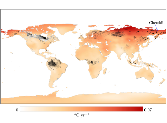
Figure 1: (Colourscale) Historical global rates of warming from the period 1951-1980 to the period 2017-2021 obtained using observations compiled by Berkeley Earth [4, 52], together with (black and gray) the global distribution of peat soils obtained from PEATMAP [72]. Note the largest warming rates at higher latitudes, in areas with a significant concentration of peat soils, such as (blue arrow) Cherskii in Northern Siberia.

In the first, mathematical modelling part of the paper in Sections 2 and 3, we:

• Modify the conceptual model introduced by Luke and Cox [36] with a more realistic microbial soil respiration function.

• Show that the modified conceptual model has a new alternative hot metastable state and reproduces the key features of the medium-complexity model from [28, Fig.4(a)].

• Demonstrate R-tipping to the hot metastable state in the modified conceptual model for realistic climate change scenarios including global warming and summer heatwaves.

• Based on the above, propose an explanation for “Zombie fires” in peatlands [3, 55, 39, 63].

In the second, mathematical analysis part of the paper in Sections 4–7, we identify non-obvious dynamical mechanisms that are responsible for the R-tipping instability to the hot metastable state. The main obstacles to analysis of this instability are twofold: the conceptual soil-carbon model is a nonautonomous dynamical system, so it does not have any equilibria or compact invariant sets, and the R-tipping is due to crossing an elusive quasithreshold in the phase space [41, 48]. To overcome these obstacles we combine three different strategies. Firstly, we consider external inputs that decay to a constant at infinity. Secondly, we compactify the problem to include the equilibrium base states for the autonomous limit systems from infinity [71]. These two strategies alone work for R-tipping due to crossing regular thresholds that are anchored at infinity by unstable compact invariant sets called regular R-tipping edge states [70, Sec.4]. However, quasithresholds do not contain such edge states [70, Sec.8]. Therefore, thirdly, we exploit large timescale separation in the model and apply concepts from geometric singular perturbation theory (GSPT). Specifically, we:

• Define R-tipping due to crossing a quasithreshold in the nonautonomous system in terms of slow manifolds and canard trajectories [68] for the autonomous compactified system.

• Identify singular R-tipping edge states: special points called folded singularities [58] that arise in the reduced (slow) system, and new saddle equilibria that arise in the layer (fast) system.

• Reduce an R-tipping problem due to crossing a quasithreshold to a heteroclinic orbit connecting the base state for the past limit system to a singular R-tipping edge state. We then use this reduction to identify four different cases of tracking-tipping transition:

  • For global warming, three (slow) cases are identified via unfolding of a codimension-two non-central heteroclinic folded saddle-node type-I singularity that arises in the reduced system.

  • For a summer heatwave, a fourth (fast) case is identified via analysis of a codimension-one heteroclinic orbit connecting the base state for the past limit system to a new saddle equilibrium that arises in the layer system.

• Show that a quasithreshold gives rise to critical ranges of rate of change of the external input rather than isolated critical rates. Furthermore, we reveal new types of quasithresholds through analysis of canard trajectories associated with singular R-tipping edge states.

2 The Nonautonomous Soil-Carbon Model

The starting point of our analysis is a discussion of the conceptual soil-carbon model introduced by Luke and Cox [36]. This model describes the time evolution of the soil temperature $T$ and soil carbon concentration $C$ in peat soils

$$\mu\frac{dT}{dt} =-\lambda(T-T_{a}(rt))+A\,C\,R_{s}(T),$$ (1)

$$\frac{dC}{dt} =\Pi-C\,R_{s}(T).$$ (2)

The model incorporates three soil processes and one time-varying external input. The first process describes balancing of the soil, $T$, and atmospheric, $T_{a}$, temperatures towards a thermal equilibrium according to Newton’s Law of Cooling, at a rate that depends on the soil-to-atmosphere heat transfer coefficient $\lambda$ and the specific heat capacity of the soil $\mu$. The second process describes a linear increase in the soil carbon concentration $C$ over time at a rate $\Pi$, due to carbon generated from decaying plant litter and other processes referred to as “Gross Primary Production” [53]. The third and only nonlinear process in the model describes temperature-sensitive microbial activity in the soil in terms of the soil respiration function $R_{s}(T)$. This process couples the dynamics of $T$ and $C$, and is discussed in detail in section 22.1. Atmospheric temperature $T_{a}(rt)$ is a time-varying external input, which represents weather anomalies or climate variation. The rate parameter $r>0$ quantifies the time scale of climatic variability and is the key input parameter in the model. An important aspect of our study is that we use realistic values of the soil parameters based on [36], which are given in Table 1 in the electronic appendix, a realistic soil respiration function $R_{s}(T)$ introduced in section 22.1, and realistic climate-change scenarios $T_{a}(rt)$ based on real weather data from Cherskii in Siberia [2]; see the arrow in fig. 1.

To facilitate the analysis, we introduce a small parameter $\epsilon=\mu/A\ll 1$ and rewrite the soil-carbon model (1)–(2) as a fast-slow nonautonomous dynamical system [69]:

$$\epsilon\frac{dT}{dt} =f_{1}(T,C,T_{a}(rt)):=-\frac{\lambda}{A}(T-T_{a}(rt))+C\,R_{s}(T),$$ (3)

$$\frac{dC}{dt} =f_{2}(T,C)\quad\quad\quad\,:=\Pi-C\,R_{s}(T),$$ (4)

where we define $f_{1}$ and $f_{2}$ for convenience. Note that system (1)–(2) or (3)–(4) does not have any equilibria (stationary solutions) owing to the time-varying external input $T_{a}(rt)$.

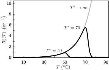
Figure 2: (Black) The modified non-monotone microbial soil respiration function $R_{s}^{*}(T)$ in (6) with $c=10$ and the die-off temperature $T^{*}=50^{\circ}$C and $70^{\circ}$C. (Grey) In the limit $T^{*}\to\infty$, we recover the unmodified monotone microbial soil respiration function $R_{s}^{\dagger}(T)$ in (5). See Table 1 in the electronic appendix for other parameter values.

2.1 Modified Microbial Respiration

Our contribution to the model introduced by Luke and Cox is a modification of the microbial soil respiration function from [36]. At low to moderate soil temperatures $T$, microbial soil respiration can be described by a $Q_{10}$ exponential function [30]:

$$R_{s}^{\dagger}(T)=R_{s}(0)\,e^{\alpha T}\quad\mbox{with}\quad\alpha=\ln{(Q_{10})}/10,$$ (5)

where the dimensionless, soil-specific parameter $Q_{10}$ may be estimated from experimental data [30]. While the monotone $R_{s}^{\dagger}(T)$ in (5) captures thermal runaway - the process responsible for the R-tipping instability, it becomes unrealistic at high $T$. Specifically, $T$ quickly increases to unrealistically high levels due to microbial soil respiration alone [36, 69]. To address this issue, we account for an important limitation, that is, soil microbes die above some die-off temperature $T=T^{*}$. Specifically, we construct a modified non-monotone microbial soil respiration function

$$R^{*}_{s}(T)={R}_{s}(0)\,\frac{e^{\alpha b}+e^{-c\alpha b}}{e^{-\alpha(T-b)}+e^{c\alpha(T-b)}}\quad\mbox{with}\quad b=T^{*}+\frac{\ln{c}}{\alpha+c\alpha},$$ (6)

that agrees with the $Q_{10}$ exponential growth (5) for $T<T^{*}$, has a maximum at $T=b\approx T^{*}$, and decays exponentially for $T>T^{*}$; see fig. 2. Such $R^{*}_{s}(T)$ captures thermal runaway and, additionally, stops it at high but realistic levels of $T$. This construction introduces two additional parameters, namely the die-off temperature $T^{*}$, and the ratio $c$ of the exponential decay rate for $T>T^{*}$ and exponential growth rate $\alpha$ for $T<T^{*}$. In the remainder of the paper, we use

$$R_{s}(T)=R_{s}^{*}(T).$$

2.2 The Autonomous Frozen System and the Moving Equilibrium

To gain insight into the tipping mechanisms in the nonautonomous system (3)–(4), or equivalently system (1)–(2), we set $r=0$ and consider properties of the resulting autonomous frozen system with fixed-in-time $T_{a}$. The frozen system has just one equilibrium

$$e(T_{a}) =(T^{e}(T_{a}),C^{e}(T_{a}))=\left(T_{a}+\frac{A\Pi}{\lambda},\frac{\Pi}{R_{s}(T_{a}+\frac{A\Pi}{\lambda})}\right),$$ (7)

which is the “base state” described in the introduction. The position of $e(T_{a})$ in the phase plane $(T,C)$ changes with $T_{a}$, but the equilibrium remains linearly stable and globally attractive (attracts all initial conditions) within the realistic range of $T_{a}$ used in our study. Thus, we can exclude the possibility of B-tipping from $e(T_{a})$ [8]. Next, we consider the stable equilibrium of the frozen system parameterised by time $t$ for a given input $T_{a}=T_{a}(rt)$, which we denote

$$e(T_{a}(rt)),$$ (8)

and refer to as the moving stable equilibrium [43, 70]. The moving stable equilibrium is not a solution to the nonautonomous system (3)–(4). However, it can serve as a useful point of reference. We follow the approach of [9, 43, 70] and relate solutions of the nonautonomous system (3)–(4) to $e(T_{a}(rt))$ for different rates $r>0$. For small $r$, solutions to (3)–(4) started near $e(T_{a}(rt))$ are guaranteed to stay near or track $e(T_{a}(rt))$ [70, Th.7.1]. However, a nonautonomous R-tipping instability in the form of a large transient departure from $e(T_{a}(rt))$ may appear for larger $r$.

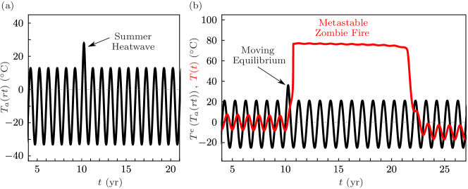
Figure 3: (a) Seasonal variations of atmospheric temperature $T_{a}(rt)$ with a summer heatwave in year 10, based on observations at Cherskii in Northern Siberia [2]. (b) Time evolution of (black) moving equilibrium soil temperature $T^{e}(T_{a}(rt))$ from (7) and (red) the actual soil temperature $T(t)$ obtained by solving (3)–(4) with the input $T_{a}(rt)$ from panel (a). The model is initialised at $t=-10\,$yr, and initial soil temperature is $T(-10)=-10^{\circ}$C. Initial soil carbon $C(-10)=120$ kg m^-2 corresponds to $\approx 3.64$ m soil depth assuming a volumetric carbon density of $33$ kg m^-3 [28, 75]. $R_{s}(T)=R_{s}^{*}(T)$ given in (6) with $T^{*}=70^{\circ}$C. See the electronic appendix for other parameter values in Table 1 and details of $T_{a}(rt)$ in section 1.3.

3 R-tipping to a Hot Metastable State and Zombie Fires

The more realistic $R_{s}(T)=R_{s}^{*}(T)$ introduced in section 2 gives rise to a hot metastable state at high soil temperatures $T\approx T^{*}$. This state is reminiscent of “Zombie fires” observed in tropical and arctic peatlands [3, 55, 39, 63]: such fires appear to be extinguished, but smoulder underground throughout the winter and re-emerge the following year [55]. Zombie fires are generally believed to happen as a result of surface wildfires [3]. However, as far as we know, there have been no attempts to explain this phenomenon. Here, we propose a hypothesis that R-tipping to a subsurface hot metastable state due to atmospheric warming is a main cause of Zombie fires. Our hypothesis is based on two remarkable results of the soil-carbon model (3)–(4) for realistic soil parameters and different climate-change scenarios $T_{a}(rt)$ based on real weather data [2].

R-tipping to a hot metastable state in the conceptual model (3)–(4) can be triggered by realistic climate patterns ranging from summer heatwaves to global warming scenarios. Figure 3 shows the soil temperature change in response to seasonal variations of the atmospheric temperature. Rather amazingly, a summer heatwave in year 10 breaks the seasonal response pattern and triggers a sudden transition to a hot metastable state that lasts for over a decade and releases most of the carbon from the soil into the atmosphere. Following this, the system settles to a lower than initial soil temperature pattern for a refractory period of over a century, during which time both soil carbon and soil temperature slowly increase back to their initial seasonal patterns. Figure 4 shows the mean soil temperature change in response to a slow increase in the mean atmospheric temperature of $4^{\circ}$C over 200 years. In this scenario, a sudden transition to a hot metastable state that lasts for over a decade is triggered, and astonishingly occurs after only a modest mean temperature increase of $\approx 1.1^{\circ}$C. Following this, the system settles to a lower than initial soil temperature for a refractory period of over a century, during which time both soil carbon and soil temperature slowly increase to their moving equilibrium levels.

R-tipping to a hot metastable state in the conceptual model (3)–(4) shows qualitative and quantitative agreement with the results of intermediate-complexity PDE models. The conceptual Ordinary Differential Equation (ODE) model (3)–(4) with the more realistic $R_{s}(T)=R_{s}^{*}(T)$ captures the key nonlinearities of the soil-carbon system. This is evidenced by the ODE model reproducing both qualitatively and quantitatively the peat soil instability predicted by a medium-complexity Partial Differential Equation (PDE) model of Siberian permafrost carbon dynamics under climate change [28, 29]. Specifically, fig. 5 shows that the ODE model manages to capture the four key features of the PDE dynamics: permafrost thawing, R-tipping to the hot metastable state that lasts for half a century, followed by a sudden soil cooling to slightly above the air temperature.

Figure 4: (a) A realisation within the range of uncertainty of the “very stringent” low-emissions RCP2.6 global warming scenario for Arctic regions [46, 45], based on observations at Cherskii in Northern Siberia [2]. (b) Time evolution of (black) the moving equilibrium soil temperature $T^{e}(T_{a}(rt))$ from (7) and (red) the actual soil temperature $T(t)$ obtained by solving (3)–(4) with the input $T_{a}(rt)$ from panel (a). Initial soil temperature is $T(0)=T_{a}^{-}+\frac{A\Pi}{\lambda}\approx-1.95^{\circ}$C. Initial soil carbon $C(0)=120$ kg m^-2 and $R_{s}(T)$ is the same as in fig. 3. See the electronic appendix for other parameter values in Table 1 and details of $T_{a}(rt)$ in section 1.4.

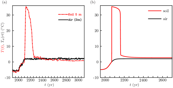
Figure 5: (a) The output of a PDE model [29] parameterised by data from near Cherskii in Siberia to simulate a soil column with a depth of 12m and a volumetric carbon density of $33$ kg m^-3, reproduced from [28, Fig.4(a)]. Shown are time evolution of (black) air temperature at 2 metres above the ground, and (red) soil temperature at a depth of 5m. (b) Time evolution of (red) the soil temperature $T(t)$ obtained by solving (3)–(4) with the (black) input $T_{a}(rt)$. For comparison with (a), we use $\Pi=0.09$ kg m^-2 yr^-1, $R_{s}(T)=0$ for $T\leq 0$ as in [28], and $R_{s}(T)=R_{s}^{*}(T)$ given in (6) with $T^{*}=30^{\circ}$C for $T>0$. Initial soil temperature is $T(0)=-6^{\circ}$C. Initial soil carbon is $C(0)=396$ kg m^-2, which corresponds to a soil column with a depth of $12$ m and a volumetric carbon density of $33$ kg m^-3 matching [28]. See the electronic appendix for other parameter values in Table 1 and details of $T_{a}(rt)$ in section 1.5.

4 The Multiscale Autonomous Compactified System

To analyse and understand non-obvious dynamical mechanisms that are responsible for the R-tipping instabilities in figs. 3 and 4, we:

• Consider external inputs $T_{a}(rt)$ that tend exponentially to a constant at infinity.

• Reformulate the ensuing two-dimensional nonautonomous system (3)–(4) as a three-dimensional autonomous compactified system [71].

• Identify three different timescales in the soil-carbon system.

We choose to work with external inputs $T_{a}(rt)$ that decay exponentially to a constant $T_{a}^{\pm}$ as time $t$ tends to $\pm\infty$. To be precise, we follow [70, Def.6.1] and

Definition 4.1.

We say $T_{a}(rt)$ is exponentially bi-asymptotically constant if, for all $r>0$,

$$\lim_{t\to\pm\infty}T_{a}(rt)=T_{a}^{\pm}\in\mathbb{R}\;\;\;\mbox{and}\;\;\lim_{t\to\pm\infty}\frac{dT_{a}(rt)/dt}{e^{\mp\rho rt}}\in\mathbb{R},$$

for some decay coefficient $\rho>0$.

Thus, we can define the autonomous past limit system with $T_{a}(rt)=T_{a}^{-}$,

$$\epsilon\,\frac{dT}{dt}=f_{1}(T,C,T_{a}^{-}),\quad\quad\frac{dC}{dt}=f_{2}(T,C),$$ (9)

and the autonomous future limit system with $T_{a}(rt)=T_{a}^{+}$,

$$\epsilon\,\frac{dT}{dt}=f_{1}(T,C,T_{a}^{+}),\quad\quad\frac{dC}{dt}=f_{2}(T,C),$$ (10)

which are examples of the frozen system. We note that, unlike the nonautonomous system (3)–(4), the autonomous past (9) and future (10) limit systems contain the equilibria

$$e^{-}:=e(T_{a}^{-})\quad\mbox{and}\quad e^{+}:=e(T_{a}^{+}),$$ (11)

respectively, and $e(T_{a}(rt))\to e^{\pm}$ as $t\to\pm\infty$ for any $r>0$.

In the next step, we include these limit systems and their equilibria in the model; see [70, 71] and section 2 of the electronic appendix for full details. We introduce a bounded dependent variable

$$s=g_{\nu}(rt)=\tanh\left(\frac{\nu}{2}\,rt\right)\in(-1,1),$$ (12)

and reformulate the two-dimensional nonautonomous system (3)–(4) on $\mathbb{R}^{2}$ as a three-dimensional autonomous compactified system on the extended phase space $\mathbb{R}^{2}\times[-1,1]$,

$$\epsilon\;\frac{dT}{dt} =f_{1}(T,C,T_{a}^{\nu}(s)),$$ (13)

$$\frac{dC}{dt} =f_{2}(T,C),$$ (14)

$$\frac{1}{r}\;\frac{ds}{dt} =\frac{\nu}{2}(1-s^{2}),$$ (15)

with the continuously extended external input

$$T_{a}^{\nu}(s)=\left\{\begin{array}[]{rcl}T_{a}\left(g^{-1}_{\nu}(s)\right)&\text{for}&s\in(-1,1),\\ T_{a}^{+}&\text{for}&s=1,\\ T_{a}^{-}&\text{for}&s=-1,\end{array}\right.$$ (16)

and compactification parameter $\nu$. A particular advantage of compactification is that the flow-invariant planes

$$\mathbb{R}^{2}\times\{-1\}\quad\mbox{and}\quad\mathbb{R}^{2}\times\{1\},$$ (17)

of the extended phase space contain equilibria $e^{-}$ and $e^{+}$ of the autonomous past (9) and future (10) limit systems, respectively. When embedded in the extended phase space, $e^{-}$ gains one unstable eigendirection with positive eigenvalue $\nu\,r>0$ and becomes a hyperbolic saddle,

$$\tilde{e}^{-}={\left(e^{-},-1\right)},$$ (18)

whereas $e^{+}$ gains one additional stable eigendirection with negative eigenvalue $-\nu\,r<0$ and becomes a hyperbolic sink, which is the only attractor for the compactified system (13)–(15),

$$\tilde{e}^{+}={\left(e^{+},+1\right)}.$$ (19)

Furthermore, we note that the moving equilibrium $e(T_{a}(rt))$ with $t\in\mathbb{R}$ corresponds to

$$\tilde{e}(s):=\left(e(T_{a}\left(g^{-1}_{\nu}(s)\right),s\right)~{}\mbox{with}~{}s\in(-1,1),$$

in (13)–(15), and $\tilde{e}(s)\to\tilde{e}^{\pm}$ as $s\to\pm 1$.

The left-hand side of the compactified system (13)–(15) shows that the soil-carbon system may evolve on up to three different timescales, depending on the rate parameter $r$. The slow time $t$ is the timescale of the slow variable $C$. The fast time $\tau=t/\epsilon$ is the timescale of the fast variable $T$. The third time $u=rt$ is the timescale of the external input $T_{a}(rt)$, which is represented by the additional variable $s$. The magnitude of the third time $u$ relative to $t$ and $\tau$ depends on the magnitude of the rate parameter $r$. Here, we consider different two-timescale limits of this three-timescale problem. A more unifying view of the system dynamics can be obtained through analysis of the three-timescale problem [15] [Sec.6, electronic appendix], which is beyond the scope of this paper.

5 Defining R-tipping due to Crossing a Quasithreshold

The multiple-timescale soil-carbon system can be viewed as a singular perturbation problem [34]. In this section, we combine compactification with concepts and techniques of GSPT to:

• Define R-tipping due to crossing a quasithreshold in the soil-carbon system (3)–(4).

• Give intuition for when to expect such R-tipping.

It is convenient to start the discussion with the autonomous frozen system obtained by setting $r=0$ in system (3)–(4), so that $T_{a}$ becomes a fixed-in-time input parameter. The frozen system is a 1-fast 1-slow singular perturbation problem with a small parameter $\epsilon$. Taking the limit $\epsilon\to 0$ in the slow time $t$ gives a singular reduced problem

$$\begin{split}\frac{dC}{dt}&=f_{2}(T,C),\end{split}$$ (20)

with slow timescale solutions restricted to the one-dimensional critical manifold

$$S(T_{a})=\left\{(T,C)~{}:~{}f_{1}(T,C,T_{a})=0\right\}\subset\mathbb{R}^{2}.$$

Taking the limit $\epsilon\to 0$ in the fast time $\tau=t/\epsilon$ gives a regular layer problem

$$\begin{split}\frac{dT}{d\tau}&=f_{1}(T,C,T_{a}),\end{split}$$ (21)

with fast timescale solutions for a fixed-in-time $C$. Note that, for a given $T_{a}$, the critical manifold $S(T_{a})$ consists of all branches of equilibria of the layer problem (21) parameterised by $C$. Hence, stability analysis of these equilibria gives stability of different parts of $S(T_{a})$. Specifically, $S(T_{a})$ has two normally hyperbolic attracting branches, denoted $S_{1}(T_{a})$ and $S_{3}(T_{a})$, which are separated from a normally hyperbolic repelling branch $S_{2}(T_{a})$ by two non-hyperbolic fold points, denoted $F_{1}(T_{a})$ and $F_{2}(T_{a})$. The attracting branch $S_{1}(T_{a})$ contains the base state $e(T_{a})$. The other attracting branch, $S_{3}(T_{a})$, is the hot metastable state that arises from the non-monotone microbial respiration function (6). The aim of GSPT is to combine the slow and fast timescale solutions for $\epsilon=0$, shown in fig. 6 (a), into slow-fast composite solutions for $0<\varepsilon<1$, shown in fig. 6 (b). We point out one particular combination: the (blue) special candidate trajectory $\theta$.

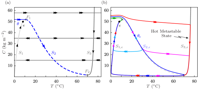
Figure 6: (a) The critical manifold $S(T_{a})$ with (grey) two normally hyperbolic attracting branches, $S_{1}(T_{a})$ and $S_{3}(T_{a})$, and (dashed blue) a normally hyperbolic repelling branch $S_{2}(T_{a})$, for the frozen system with $T_{a}=0$ and $\epsilon=0$. Shown also are (single arrows) slow timescale trajectories of the reduced problem (20) along $S(T_{a})$, and (double arrows) fast timescale trajectories of the layer problem (21) for different values of $C$. (b) Five fast-slow composite trajectories in the autonomous frozen system with $T_{a}=0$, $\epsilon\approx 0.064$, the same initial soil temperature $T(0)=0$, and different initial carbon levels: (green) $C(0)=53$, (cyan) $C(0)=54.287996178057110079$, (blue) $C(0)\approx 54.28799617805711008$, (magenta) $C(0)=54.287996178057110088$, and (red) $C(0)=55.5$. Included for reference is (grey) $S(T_{a})$. See Table 1 in the electronic appendix for other parameter values.

For $0<\epsilon\ll 1$, the normally hyperbolic parts of $S(T_{a})$ are guaranteed by the ‘first’ Fenichel theorem to perturb smoothly to nearby normally hyperbolic and locally invariant slow manifolds [22, 23, 27, 68, 34]. To be specific, $S_{1}(T_{a})$ and $S_{3}(T_{a})$ perturb to nearby attracting slow manifolds $S_{1,\epsilon}(T_{a})$ and $S_{3,\epsilon}(T_{a})$. Similarly, $S_{2}(T_{a})$ perturbs to a nearby repelling slow manifold $S_{2,\epsilon}(T_{a})$. Each slow manifold is usually non-unique in the sense that there is a family of such slow manifolds that lie exponentially close in $\epsilon$ to each other; see [68, Th.3.1] and [34, Th.3.1.4]. The strategy is to fix a representative for each of these manifolds and work with these representatives. Near the non-hyperbolic fold points $F_{1}(T_{a})$ and $F_{2}(T_{a})$, the hyperbolic branches $S_{1,\epsilon}(T_{a})$, $S_{3,\epsilon}(T_{a})$ and $S_{2,\epsilon}(T_{a})$ typically split, meaning that they typically become slow manifolds with either one or two boundaries. In particular, $S_{1,\epsilon}(T_{a})$ has one inflow boundary near $F_{1}(T_{a})$, $S_{3,\epsilon}(T_{a})$ has one outflow boundary near $F_{2}(T_{a})$, while $S_{2,\epsilon}(T_{a})$ has one inflow boundary near $F_{1}(T_{a})$ and one outflow boundary near $F_{2}(T_{a})$. Local invariance means that trajectories can enter or leave a slow manifold only through its boundary. Furthermore, the splitting of $S_{1,\epsilon}(T_{a})$ and $S_{2,\epsilon}(T_{a})$ near $F_{1}(T_{a})$ gives rise to a narrow continuum of special solutions, referred to as canards, that move along $S_{2,\epsilon}(T_{a})$ for some time $t$ [10, 21, 31, 58, 68]; see fig. 6 (b). In the remainder of the paper we follow [67, 11] and [68, Sec.3.2.4] and identify three different types of canards.

Definition 5.1.

In the autonomous frozen system and in the autonomous compactified system (13)–(15):

• Canards “without head” are solutions, or the corresponding trajectories, that move slowly along $S_{2,\epsilon}$ for time $t={\cal{O}}(1)$ before moving quickly and directly to $S_{1,\epsilon}$.

• Canards “with head” are solutions, or the corresponding trajectories, that move slowly along $S_{2,\epsilon}$ for time $t={\cal{O}}(1)$, then move quickly and directly to $S_{3,\epsilon}$, then move slowly along $S_{3,\epsilon}$, before converging to $S_{1,\epsilon}$.

• A maximal canard is a special solution, or the corresponding trajectory, that enters $S_{2,\epsilon}$ through its inflow boundary.

Examples of a maximal canard, denoted $\theta_{\epsilon}$, a canard “without head” and a canard “with head” in the frozen system are shown in blue, cyan and magenta, respectively, in fig. 6 (b). The (blue) maximal canard $\theta_{\epsilon}$ is a special example of a canard without head, and a perturbation of the special candidate trajectory $\theta$. In practice, a maximal canard is computed by choosing a suitable arclength and finding the trajectory along $S_{2}(T_{a})$ that takes the longest time to trace out this arclength.

The above discussion identifies two obstacles to defining R-tipping to the hot metastable state. First, the hot metastable state is a transient and thus quantitative phenomenon. In the long term, the system converges to the same stable state $e^{+}$ for any rate $r>0$. Second, there is no unique threshold for R-tipping to the hot metastable state [70]. Rather, one speaks of a “quasithreshold” comprising a family of canards. GSPT together with compactification allow us to overcome both of these obstacles.

We focus on R-tipping from $e^{-}$ and relate nonautonomous and compactified system dynamics. Using the notation $x=(T,C)\in\mathbb{R}^{2}$ for the state variable of the soil-carbon system, we write

$$x^{[r]}(t,e^{-})\in\mathbb{R}^{2},$$ (22)

to denote the unique solution to the nonautonomous system (3)–(4) at time $t$, that limits to $e^{-}$ as $t\to-\infty$ for a given rate parameter $r$. We also write $W^{u,[r]}(\tilde{e}^{-})$ to denote the unique rate-dependent one-dimensional unstable invariant manifold of the hyperbolic saddle $\tilde{e}^{-}$ in the autonomous compactified system (13)–(15). It follows from [70, Prop.6.4(a)] that $W^{u,[r]}(\tilde{e}^{-})$ contains ${x}^{[r]}(t,{e}^{-})$ in the sense that

$$W^{u,[r]}(\tilde{e}^{-})\supset\left\{(x,s)~{}:~{}x=x^{[r]}(t,e^{-}),~{}s=g_{\nu}(t)\right\}_{t\in\mathbb{R}}.$$ (23)

This relation allows us to define tracking and R-tipping for the nonautonomous system (3)–(4) in terms of $W^{u,[r]}(\tilde{e}^{-})$ and slow manifolds in the autonomous compactified system (13)–(15):

Definition 5.2.

Consider the nonautonomous system (3)–(4) with exponentially bi-asymptotically constant $T_{a}(rt)$ and decay coefficient $\rho>0$, and the corresponding autonomous compactified system (13)–(15) with the compactification parameter $\nu\in(0,\rho]$. For a fixed $r>0$:

• We say $x^{[r]}(t,e^{-})$ tracks the moving stable equilibrium $e(T_{a}(rt))$ in system (3)–(4) if $W^{u,[r]}(\tilde{e}^{-})$ connects to $\tilde{e}^{+}$ directly, i.e. without visiting $S_{2,\epsilon}$ or $S_{3,\epsilon}$, in system (13)–(15).

• We say $x^{[r]}(t,e^{-})$ R-tips in system (3)–(4), or say system (3)–(4) R-tips from $e^{-}$, if $W^{u,[r]}(\tilde{e}^{-})$ visits $S_{3,\epsilon}$ before connecting to $\tilde{e}^{+}$ in system (13)–(15).

Since R-tipping is not the complement of tracking, the nonautonomous system (3)–(4) with $0<\epsilon\ll 1$ does not have unique R-tipping thresholds separating trajectories that track the moving stable equilibrium from those that R-tip, and does not have isolated critical rates $r$. More precisely:

Definition 5.3.

Consider the nonautonomous system (3)–(4) with exponentially bi-asymptotically constant $T_{a}(rt)$ and decay coefficient $\rho>0$, and the corresponding autonomous compactified system (13)–(15) with the compactification parameter $\nu\in(0,\rho]$.

• We define a critical range of $r$ as an interval of $r$ for which $x^{[r]}(t,e^{-})$ neither tracks the moving stable equilibrium $e(T_{a}(rt))$ nor R-tips.

• For a fixed $r>0$, we define an R-tipping quasithreshold in system (13)–(15) as a family of canards “without head” including a maximal canard, and in system (3)–(4) as a family of solutions $x^{[r]}(t)$ or trajectories corresponding to this family of canards.

Remark 5.1.

There are important differences between R-tipping quasithresholds defined above and regular R-tipping thresholds introduced in [70, Def.5.3]. We refer to section 3 of the electronic appendix for more details.

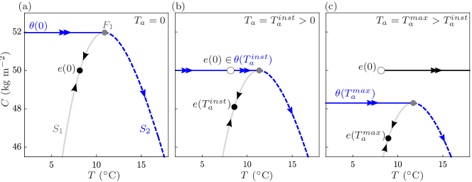
Figure 7: Phase portraits of the frozen system with $\epsilon=0$ for three different values of $T_{a}$ show when to expect R-tipping in the nonautonomous system (3)–(4) with $0<\epsilon\ll 1$ and a time-varying $T_{a}$. Note the change in the position of the (blue) special candidate trajectory $\theta(T_{a})$ for different values of $T_{a}$ relative to the fixed initial base state $e(0)$ at $T_{a}=0$.

To give intuition for when to expect R-tipping due to crossing a quasithreshold in the nonautonomous system (3)–(4), we extend the concept of threshold instability, introduced in [70, Def.4.5] for regular thresholds, to quasithresholds. Consider phase portraits of the frozen system in the limit $\epsilon=0$ for three different values of $T_{a}$ in fig. 7. Suppose that $T_{a}=0^{\circ}$C and the system is settled at the base state $e(0)$; see fig. 7 (a). Then, there is a special value of $T_{a}$, derived in section 4 of the electronic appendix,

$$T_{a}=T_{a}^{inst}\approx-\frac{1}{\alpha}\left(1+\log{\left(\alpha\frac{A\Pi}{\lambda}\right)}-\alpha\frac{A\Pi}{\lambda}\right),$$ (24)

such that the base state for $T_{a}=0$ crosses the special candidate trajectory for $T_{a}=T_{a}^{inst}>0$, that is $e(0)\in\theta(T_{a}^{inst})$; see fig. 7 (b). If $T_{a}$ switches discontinuously from $0$ to $T_{a}^{max}$, then $e(0)$ becomes the initial condition for the frozen system with $T_{a}=T_{a}^{max}$. Thus, following a switch to $T_{a}^{max}>T_{a}^{inst}$, $e(0)$ will find itself on the other side of the special candidate trajectory $\theta(T_{a}^{max})$ and the system will undergo R-tipping; see fig. 7 (c). In Sections 6 and 7, we relate condition (24) to R-tipping conditions for $0<\epsilon\ll 1$ and continuously varying $T_{a}(rt)$.

6 R-tipping Mechanisms for Global Warming

The R-tipping instability in fig. 4 arises because time-variation of the mean atmospheric temperature $T_{a}$ interacts with the slow timescale of soil carbon $C$. Thus, to uncover the underlying dynamical mechanisms, we consider the 1-fast 2-slow system (13)–(15) with the rate parameter $r\lesssim 1$, where $u=rt\lesssim t$ becomes another slow time and $s$ becomes another slow variable.

The singular reduced problem, obtained by setting $\epsilon=0$ for the slow time $t$ in (13)–(15),

$$\frac{dC}{dt} =f_{2}(T,C),$$ (25)

$$\frac{ds}{dt} =\frac{r}{2}\,(1-s^{2}),$$ (26)

gives slow timescale solutions evolving on a two-dimensional critical manifold

$$S=\left\{(T,C,s)~{}:~{}f_{1}(T,C,T_{a}^{1}(s))=0\right\}\subset\mathbb{R}^{2}\times[-1,1].$$ (27)

$S$ consists of two normally hyperbolic attracting sheets, $S_{1}$ containing $\tilde{e}(s)$, and $S_{3}$ being the hot metastable state, which are separated from a normally hyperbolic repelling sheet $S_{2}$ by two non-hyperbolic fold curves $F_{1}$ and $F_{2}$ (see fig. 8 (b)). The regular layer problem, obtained by setting $\epsilon=0$ for the fast time $\tau=t/\epsilon$,

$$\frac{dT}{d\tau} =f_{1}(T,C,T_{a}^{\nu}(s)),$$ (28)

gives fast timescale solutions along straight lines for fixed-in-time $C$ and $s$.

As a model of the global warming scenario, we consider a slow nonlinear shift from $T_{a}^{-}=0^{\circ}$C to a given $T_{a}^{+}>0$, that decays exponentially with the decay coefficient $\rho=2$ as per definition 4.1,

$$T_{a}(rt)=\frac{T_{a}^{+}}{2}\,(\tanh{(rt)}+1).$$ (29)

We then fix the compactification parameter $\nu=1$ and apply the inverse of the compactification transformation (12) to (29) to obtain

$$T_{a}^{\nu}(s)=T_{a}^{1}(s)=\frac{T_{a}^{+}}{2}\,\frac{(1+s)^{2}}{1+s^{2}}.$$ (30)

To give an overview of the dynamics near transitions from tracking to R-tipping, we plot in fig. 8 (a) an R-tipping diagram in the plane $(T_{a}^{+},r)$ of the input parameters. The diagram was obtained by computing $W^{u,[r]}(\tilde{e}^{-})$ in system (13)–(15) with $0<\epsilon\ll 1$ for different values of $T_{a}^{+}$ and $r$, and using Defs. 5.1–5.3 to identify different dynamical regions for system (3)–(4). There are two R-tipping regions, and one tracking-tipping transition found for a large enough shift magnitude $T_{a}^{+}$. The smaller R-tipping region is a curious R-tipping tongue. This tongue gives rise to two (cyan) critical ranges of $r$ for a fixed $T_{a}^{+}$ (one of them being very narrow), and different tracking-tipping transitions for low and high magnitudes $T_{a}^{+}$ of the shift.

To gain geometric insight into the R-tipping instability caused by global warming, we plot in fig. 8 (b) the unstable manifold $W^{u,[r]}(\tilde{e}^{-})$ for a fixed $T_{a}^{+}=5^{\circ}$C and three different slow rates $0<r_{1}<r_{2}<r_{3}$ (see the black dots in fig. 8 (a)), together with the critical manifold $S$ for reference. Figure 8 (b) shows that, as $r$ is increased, tracking of $\tilde{e}(s)$ by (green) $W^{u,[r_{1}]}(\tilde{e}^{-})$ is lost via canard trajectories, including the maximal canard contained in (blue) $W^{u,[r_{2}]}(\tilde{e}^{-})$ that crosses $F_{1}$ and moves along $S_{2}$ for the longest time. This is followed by R-tipping at higher $r$ as shown by (red) $W^{u,[r_{3}]}(\tilde{e}^{-})$ that crosses $F_{1}$ and approaches the hot metastable state $S_{3,\epsilon}$ along the fast $T$-direction before connecting to $\tilde{e}^{+}$. Since R-tipping due to global warming (29) occurs when the slow timescale segment of $W^{u,[r]}(\tilde{e}^{-})$ on $S$ crosses $F_{1}$, it should be possible to explain the R-tipping diagram in fig. 8 (a), including the curious R-tipping tongue, in terms of slow timescale solutions of the two-dimensional reduced problem alone [69, 48, 62].

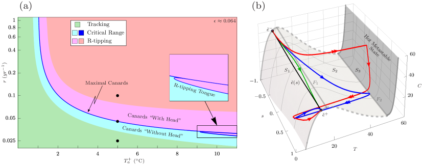
Figure 8: (a) R-tipping diagram for nonautonomous system (3)–(4) with global warming scenario (29), in the plane of the shift amplitude $T_{a}^{+}$ and the rate parameter $r$, for $\epsilon\approx 0.064$. Shown are regions of (green) tracking, (cyan, blue) critical range, and (magenta, red) R-tipping from $\tilde{e}^{-}$. (b) (Colour) The unstable invariant manifold $W^{u,[r]}(\tilde{e}^{-})$ of the saddle $\tilde{e}^{-}$ for the compactified system (13)–(15) with $\epsilon\approx 0.064$ and global warming scenario (30) with $T_{a}^{+}=5^{\circ}$C, for three different values of the rate parameter: (green) $r_{1}=0.02$ , (blue) $r_{2}\approx 0.0454218$, and (red) $r_{3}=0.1$; see the black dots in (a). Included for reference is (grey) the critical manifold $S$ defined in (27). See Table 1 in the electronic appendix for other parameter values.

6.1 The Reduced Problem and Desingularisation

The reduced problem (25)–(26) for the 1-fast 2-slow system (13)–(15) with global warming (30) describes the evolution of the slow variables $C$ and $s$ in the slow time $t$ on the two-dimensional critical manifold $S$ defined in (27). However, the onset of R-tipping involves a sudden jump in the fast variable $T$, without any noticeable change in $C$. Thus, it is convenient to consider the evolution of the fast variable $T$ in the slow time $t$ on $S$, which is obtained by differentiating the critical-manifold condition in (27) with respect to $t$. Furthermore, we use the critical-manifold condition to project the slow flow within $S$ onto the plane $(T,s)$, i.e. eliminate the dependence on $C$, and reformulate the reduced problem as

$$\frac{dT}{dt} =\left.-\frac{\partial f_{1}/\partial C\cdot f_{2}+\partial f_{1}/\partial T_{a}^{1}\cdot dT_{a}^{1}/ds\cdot ds/dt}{\partial f_{1}/\partial T}\right|_{S},$$ (31)

$$\frac{ds}{dt} =\frac{r}{2}\,(1-s^{2}),$$ (32)

where $|_{S}$ denotes restriction to $S$. In the reduced problem (31)–(32), the question of loss of tracking boils down to whether $W^{u,[r]}(\tilde{e}^{-})$ leaves $S_{1}$ through $F_{1}$. To address this question, we note that the denominator in (31) changes sign at a fold

$$\left.\frac{\partial f_{1}}{\partial T}\right|_{S}\left\{\begin{array}[]{ll}<0&\mbox{for}\quad(T,C,s)\in S_{1}\cup S_{3},\\ =0&\mbox{for}\quad(T,C,s)\in F_{1}\cup F_{2},\\ >0&\mbox{for}\quad(T,C,s)\in S_{2}.\end{array}\right.$$ (36)

It then follows that, depending on the numerator in (31), there are two types of fold points:

• A jump point [58] is a point $p$ on a fold such that

  $$\left.\left(\frac{\partial f_{1}}{\partial C}\cdot f_{2}+\frac{\partial f_{1}}{\partial T_{a}^{1}}\cdot\frac{dT_{a}^{1}}{ds}\cdot\frac{ds}{dt}\right)\right|_{p\in F_{1}\cup F_{2}}\neq 0.$$ (37)

  If a solution of (31)–(32) approaches a jump point, the denominator in (31) approaches zero while the numerator remains finite, so that $dT/dt$ tends to infinity, and $T(t)$ blows up in $t$. This means that the solution reaches a jump point in finite time and ceases to exist within $S$. Jump points are typically found on open subsets of a fold [58].

• A folded singularity [58] is a point $q$ on a fold such that

  $$\left.\left(\frac{\partial f_{1}}{\partial C}\cdot f_{2}+\frac{\partial f_{1}}{\partial T_{a}^{\nu}}\cdot\frac{dT_{a}^{\nu}}{ds}\cdot\frac{ds}{dt}\right)\right|_{q\in F_{1}\cup F_{2}}=0.$$ (38)

  If a solution of (31)–(32) approaches a folded singularity in a special direction where the numerator in (31) approaches zero faster than or at the same rate as the denominator in (31), then $dT/dt$ remains finite, and this solution either grazes or crosses the fold at $q$ with a finite speed. If the crossing is from an attracting to an unstable part of $S$, the solution, or the corresponding trajectory, is termed a singular canard [11, 10]. Folded singularities, which are typically found as isolated fold points, are examples of “singular R-tipping edge states” described in the introduction.

Thus, in the singular limit $\epsilon=0$ for the slow time $t$, transitions from tracking to R-tipping caused by global warming can be understood in terms of singular canards through folded singularities [69, 41, 48]. The obstacle to analysis of folded singularities and their singular canards is that the right-hand side of (31) is undefined on $F_{1}$ and $F_{2}$. This obstacle is overcome by a desingularisation [58, 20] in the form of a state-dependent time rescaling:

$$dt=\left.-d\hat{t}\;\frac{\partial f_{1}}{\partial T}\right|_{S},$$ (39)

which gives the desingularised system

$$\frac{dT}{d\hat{t}} =R_{s}^{*}(T)\left(\Pi-\frac{\lambda}{A}\left(T-T_{a}^{1}(s)\right)\right)+\frac{r\lambda T_{a}^{+}}{2A}\left(\frac{1-s^{2}}{1+s^{2}}\right)^{2},$$ (40)

$$\frac{ds}{d\hat{t}} =\frac{r\lambda}{2A}(1-s^{2})\left(1+\alpha\left(T-T_{a}^{1}(s)\right)\frac{ce^{c\alpha(T-b)}-e^{-\alpha(T-b)}}{e^{c\alpha(T-b)}+e^{-\alpha(T-b)}}\right),$$ (41)

defined everywhere on $S$. The main advantages of desingularisation are:

• Regular equilibria for the reduced problem (31)–(32) remain regular equilibria for the desingularised system (40)–(41). Folded singularities for (31)–(32) become (new) regular equilibria for (40)–(41). Hence the classification of folded singularities into “folded nodes”, “folded foci”, “folded saddles”, and “folded saddle-nodes”, based on their classification into different types of equillibria in (40)–(41) [58].

• According to (36) and (39), the new time $\hat{t}$ in  (40)–(41) flows in the same direction as $t$ on $S_{1}$ and $S_{3}$, passes infinitely faster on $F_{1}$ and $F_{2}$, and reverses direction on $S_{2}$. Thus, a phase portrait for (31)–(32) can be obtained by producing the corresponding phase portrait for (40)–(41), reversing the direction of time (the arrows on trajectories) on $S_{2}$, and relabelling the (new) equilibria on $F_{1}$ and $F_{2}$ as folded singularities.

• It follows from points (a1) and (a2) above that a singular canard through a folded singularity in (31)–(32) can be obtained by smoothly concatenating two trajectories tangent to a stable eigendirection of the corresponding equilibrium in (40)–(41). We refer to section 5 of the electronic appendix for the discussion of different singular canards associated with different folded singularities.

6.2 Three Slow Cases in the Reduced Problem

To be precise and consistent with Defs. 5.2 and 5.3 for $0<\epsilon\ll 1$, we now define tracking, R-tipping and critical rates for slow external inputs in the limit $\epsilon=0$ as follows:

Definition 6.1.

In the reduced problem (31)–(32), we say that:

• Tracking occurs when $W^{u,[r]}(\tilde{e}^{-})$ connects to $\tilde{e}^{+}$ directly, that is without visiting $F_{1}$.

• R-tipping occurs when $W^{u,[r]}(\tilde{e}^{-})$ reaches a jump point on $F_{1}$ and stops existing in $S$.

• A critical rate is an isolated value of $r$ that gives neither tracking nor R-tipping.

Then, we use relations (a1)–(a3) between the desingularised and reduced system dynamics to identify different tracking-tipping transitions in the singular reduced problem (31)–(32) through analysis of the unstable manifold $W^{u,[r]}(\tilde{e}^{-})$ in the regular desingularised system (40)–(41). We note that, when $r$ is sufficiently small, tracking occurs because the whole of $F_{1}$ is repelling, so $W^{u,[r]}(\tilde{e}^{-})$ must remain on $S_{1}$ and connect directly to $\tilde{e}^{+}$. As the rate parameter $r$ is increased, there is a saddle-node bifurcation of equilibria on $F_{1}$ at some $r=r_{SN}$ in (40)–(41). This bifurcation corresponds to the appearance of a folded saddle-node type-I singularity (FSN-I) [32, 64] in (31)–(32). As $r$ is increased past $r_{SN}$, FSN-I bifurcates into a folded saddle (FS) and a folded node (FN). Thus, $W^{u,[r]}(\tilde{e}^{-})$ may interact with singular canards of FS and FN to cross $F_{1}$ and cause loss of tracking. Analysis of heteroclinic orbits in (40)–(41), where $W^{u,[r]}(\tilde{e}^{-})$ connects $\tilde{e}^{-}$ to an equilibrium on $F_{1}$, reveals three different cases of loss of tracking in (31)–(32):

• The simple slow case: $W^{u,[r]}(\tilde{e}^{-})$ coalesces with the folded-saddle singular canard $\tilde{\gamma}^{S}$, and thus crosses from $S_{1}$ to $S_{2}$ via FS, at some critical rate $r=r_{c}>r_{SN}$.

• The complicated slow case: $W^{u,[r]}(\tilde{e}^{-})$ grazes $F_{1}$ at FSN-I when $r=r_{SN}$, coalesces with a folded-node weak singular canard when $r\in(r_{SN},r_{Ns})$, coalesces with the folded-node strong singular canard $\tilde{\gamma}^{N}_{s}$ at some $r=r_{Ns}>r_{SN}$, and thus crosses from $S_{1}$ to $S_{2}$ via FN when $r\in(r_{SN},r_{Ns}]$.

• The degenerate slow case: $W^{u,[r]}(\tilde{e}^{-})$ coalesces with the folded-saddle-node singular canard $\tilde{\gamma}^{SN}$, and thus crosses from $S_{1}$ to $S_{2}$ via FSN-I, at a critical rate $r_{c}=r_{SN}$.

These three cases of ‘loss of tracking’ give rise to three different cases of ‘tracking-tipping transition’, which we refer to as the three slow cases. Cases (i) and (ii) are typical and closely related to the two cases of non-obvious tipping thresholds described in separate systems in [48]. The new case (iii) is special and separates the typical cases (i) and (ii). Below, we identify all three cases in an unfolding of a codimension-two non-central heteroclinic FSN-I, which explains the problem at hand, consolidates the results of [48], and is of interest in its own right. To highlight interactions of $W^{u,[r]}(\tilde{e}^{-})$ with different singular canards, we colour $S_{1}$ in the phase portraits as follows. Solutions initialised in the green region remain in this region and converge directly to $\tilde{e}^{+}$ (tracking). Solutions initialised in the dark red region reach a jump point of $F_{1}$ and cease to exist within $S$ (R-tipping). Remaining solutions (neither tracking nor R-tipping) include: weak folded-node singular canards initialised in the yellow region (singular funnel), the folded-node strong singular canard $\tilde{\gamma}^{N}_{s}$ separating the red and yellow regions, and the folded-saddle singular canard $\tilde{\gamma}^{S}$ separating the green and red regions. Finally, in the figures, we show projections of $S$ onto the plane $(T,s)$.

6.2.1 The simple slow case

As $r$ is increased past $r_{SN}$ for $T_{a}^{+}=1.5$ in (31)–(32), the appearance of FS and FN via FSN-I gives rise to a folded-saddle singular canard $\tilde{\gamma}^{S}$, folded-node singular canards including the folded-node strong singular canard $\tilde{\gamma}^{N}_{s}$, and new dynamics; see fig. 9 (a)-(b). Of particular interest is an attracting interval of jump points on $F_{1}$ between FS and FN, and the corresponding (dark red) region of solutions between $\tilde{\gamma}^{S}$ and $\tilde{\gamma}^{N}_{s}$ that reach one of these jump points from $S_{1}$ and cease to exist within $S$. In this case, $W^{u,[r]}(\tilde{e}^{-})$ does not interact with FSN-I, meaning that the FSN-I is local. $W^{u,[r]}(\tilde{e}^{-})$ does not interact with the folded-node singular canards either because it is separated from them by $\tilde{\gamma}^{S}$. Rather, when $r=r_{c}$, $W^{u,[r]}(\tilde{e}^{-})$ and $\tilde{\gamma}^{S}$ coalesce; see fig. 9 (c). At this point, tracking is lost since $W^{u,[r]}(\tilde{e}^{-})$ crosses $F_{1}$ from $S_{1}$ to $S_{2}$ via FS. For $r>r_{c}$, $W^{u,[r]}(\tilde{e}^{-})$ reaches a jump point on $F_{1}$ and ceases to exist within $S$ so R-tipping occurs; see fig. 9 (d).

Thus, in the simple slow case for $\epsilon=0$, there is a critical rate $r=r_{c}$. This critical rate is the value of $r$ that gives a codimension-one hetroclinic orbit connecting $\tilde{e}^{-}$ to the corresponding saddle on $F_{1}$ in the desingularised system (40)–(41).

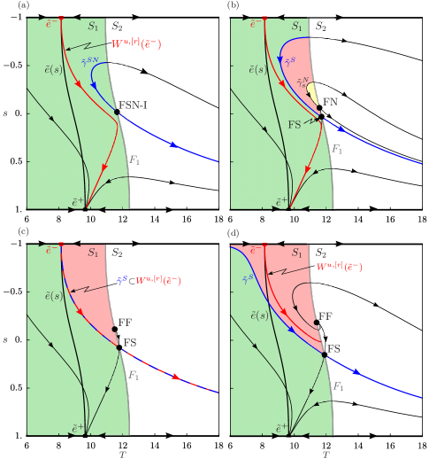
Figure 9: The simple slow case of tracking-tipping transition in phase portraits of the reduced problem (31)–(32) with nonlinear shift (30), obtained using the desingularised system (40). Note tracking in spite of a codimension-one local FSN-I in (a), and loss of tracking via a codimension-one heteroclinic orbit connecting $\tilde{e}^{-}$ to FS in (c) that leads to R-tipping in (d). $T_{a}^{+}=1.5$ and the rate parameter takes values $(a)\ r=r_{SN}\approx 0.107194,\ (b)\ r\approx 0.108119,\ (c)\ r=r_{c}\approx 0.111459,$ and $(d)\ r=0.12$; see the black dots in the left inset of fig. 12 (c). See Table 1 in the electronic appendix for other parameter values.

6.2.2 The complicated slow case

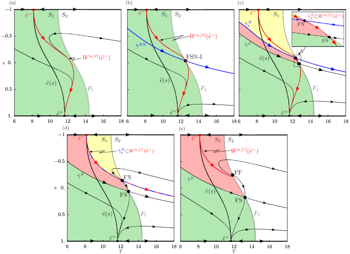
Figure 10: The complicated slow case of tracking-tipping transition in phase portraits of the reduced problem (31)–(32) with nonlinear shift (30), obtained using the desingularised system (40)–(41). Note tracking in (a), loss of tracking via a codimension-one central heteroclinic FSN-I in (b), and a codimension-one heteroclinic orbit connecting $\tilde{e}^{-}$ to FN in (d) that leads to R-tipping in (e) . $T_{a}^{+}=3.5$ and the rate parameter takes values $(a)\ r=0.045,(b)\ r=r_{SN}\approx 0.050086,\ (c)\ r\approx 0.050669,\ (d)\ r=r_{c}\approx 0.052266,$ and $(e)\ r=0.06$; see the black dots in the right inset of fig. 12 (c). See Table 1 in the electronic appendix for other parameter values.

As $r$ is increased past $r_{SN}$ for $T_{a}^{+}=3.5$, the local bifurcation scenario is the same as in the simple case: appearance of FS and FN via FSN-I gives rise to folded-saddle and folded-node singular canards, an attracting interval of jump points on $F_{1}$ between FS and FN, and the corresponding (dark red) region of solutions between $\tilde{\gamma}^{S}$ and $\tilde{\gamma}^{N}_{s}$ that reach one of these jump points from $S_{1}$ and cease to exist within $S$; see fig. 10. However, the global dynamics are different in that $W^{u,[r]}(\tilde{e}^{-})$ interacts with various folded-node singular canards. When $r=r_{SN}$, $W^{u,[r]}(\tilde{e}^{-})$ grazes $F_{1}$ at FSN-I, giving rise to a codimension-one central heteroclinic FSN-I; see fig. 10 (b). In other words, the FSN-I is global. At this point tracking is lost, but R-tipping cannot occur for $r$ just above $r_{SN}$ because $W^{u,[r]}(\tilde{e}^{-})$ passes through the yellow singular funnel and crosses $F_{1}$ from $S_{1}$ to $S_{2}$ via FN; see fig. 10 (c). Thus, $W^{u,[r]}(\tilde{e}^{-})$ contains a folded-node weak singular canard. Then, $W^{u,[r]}(\tilde{e}^{-})$ crosses $F_{1}$ back to $S_{1}$ via FS and connects to $\tilde{e}^{+}$. Thus, $W^{u,[r]}(\tilde{e}^{-})$ also contains the faux folded-saddle singular canard $\tilde{\gamma}^{S}_{f}$. For some $r=r_{Ns}>r_{SN}$, $W^{u,[r]}(\tilde{e}^{-})$ and $\tilde{\gamma}^{N}_{s}$ coalesce. At this point, $W^{u,[r]}(\tilde{e}^{-})$ crosses $F_{1}$ from $S_{1}$ to $S_{2}$ via FN and never returns to $S_{1}$; see fig. 10 (d). It is only for $r>r_{Ns}$ that $W^{u,[r]}(\tilde{e}^{-})$ reaches a jump point on $F_{1}$ and R-tipping occurs; see fig. 10 (e).

Thus, in the complicated slow case for $\epsilon=0$, there is a critical range of $r\in[r_{SN},r_{Ns}]$. The minimum of the critical range is the value of $r$ that gives a a codimension-one heteroclinic orbit connecting $\tilde{e}^{-}$ to the corresponding saddle-node on $F_{1}$ along the centre eigendirection in the desingularised system (40)–(41). The maximum of the critical range is the value of $r$ that gives a codimension-one hetroclinic orbit connecting $\tilde{e}^{-}$ to the corresponding stable node on $F_{1}$ along the strong eigendirection in (40)–(41). For $r$ in the interior of the critical range, there is a codimension-zero heteroclinic orbit connecting $\tilde{e}^{-}$ to the corresponding stable node on $F_{1}$ along the weak eigendirection in (40)–(41).

6.2.3 The degenerate slow case

A natural question to ask is: what separates the simple and complicated slow cases? It turns out that there is a special value $T_{a}^{+}=T_{a,c}^{+}$. As $r$ is increased past $r_{SN}$ for this special value of $T_{a}^{+}$, the local bifurcation scenario is the same as in the simple and complicated slow cases. However, the global dynamics are different in that $W^{u,[r]}(\tilde{e}^{-})$ interacts with the folded-saddle-node singular canard $\tilde{\gamma}^{SN}$. In contrast to the simple and complicated slow cases, if $r=r_{SN}$ and $T_{a}^{+}=T_{a,c}^{+}$, $W^{u,[r]}(\tilde{e}^{-})$ and $\tilde{\gamma}^{SN}$ coalesce, giving rise to a codimension-two non-central heteroclinic FSN-I; see fig. 11 (b). In other words, the FSN-I is global, but different from the complicated slow case. At this point, tracking is lost since $W^{u,[r_{c}]}(\tilde{e}^{-})$ crosses $F_{1}$ from $S_{1}$ to $S_{2}$ via FSN-I. For $r>r_{SN}$, $W^{u,[r]}(\tilde{e}^{-})$ reaches a jump point on $F_{1}$ and R-tipping occurs; see fig. 11 (c).

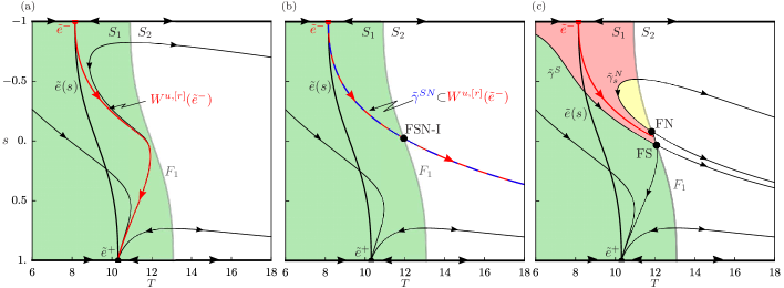
Figure 11: The degenerate slow case of tracking-tipping transition in phase portraits of the reduced problem (31)–(32) with nonlinear shift (30), obtained using the desingularised system (40)–(41). Note tracking in (a), and loss of tracking via a codimension-two non-central heteroclinic FSN-I in (b) that leads to R-tipping in (c). $T_{a}^{+}=2.15938$ and the rate parameter takes values $(a)\ r\approx 0.0716488,\ (b)\ r=r_{SN}=r_{c}\approx 0.0766488,$ and $(c)\ r\approx 0.0776488$; see the black dots in the middle inset of fig. 12. System parameter values are given in Table 1 in the electronic appendix.

Thus, in the degenerate case for $\epsilon=0$, there is neither a critical range nor a critical rate. Instead, there is a critical pair $(T_{a,c}^{+},r_{c})$. This critical pair is the combination of $r$ and $T_{a}^{+}$ that give a codimension-two heteroclinic orbit connecting $\tilde{e}^{-}$ to the corresponding saddle-node on $F_{1}$ along the stable eigendirection in the desingularised system (40)–(41).

6.3 Bringing it Together: Unfolding of Non-central Heteroclinic FSN-I

The aim of this section is twofold. First, we summarise our results from section 66.2 in the singular R-tipping diagram for $\epsilon=0$ in fig. 12 (c). Second, we use the singular R-tipping diagram to explain the regular R-tipping diagram for $\epsilon\approx 0.064$ in fig. 8 (a).

The singular R-tipping diagram is obtained by the unfolding of a codimension-two non-central heteroclinic FSN-I in the plane $(T_{a}^{+},r)$ of the input parameters in the reduced problem (31)–(32). This unfolding, in turn, is obtained by the unfolding of a codimension-two non-central saddle-node heteroclinic bifurcation in the desingularised system (40)–(41). The diagram is partitioned into regions of (green) tracking, (red) R-tipping, and (yellow) neither tracking nor R-tipping by two curves that are tangent at the special point of codimension-two non-central hetroclinic FSN-I, denoted $\tilde{e}$-to-FSN-I_s in the middle inset. Each curve has two branches emanating from the special point. Both branches of the black curve of FSN-I were obtained by computing the saddle-node bifurcation of equilibria on $F_{1}$ in (40)–(41); we will return to this curve later. The left branch of the blue curve, denoted $\tilde{e}$-to-FS, was obtained by computing a codimension-one heteroclinic orbit connecting $\tilde{e}^{-}$ to the saddle on $F_{1}$ in (40)–(41). This connection gives a critical rate in the simple slow case for the reduced problem (31)–(32), where $W^{u,[r]}(\tilde{e}^{-})\supset\tilde{\gamma}^{S}$; see fig. 9 (c). Note that $\tilde{e}$-to-FS has a vertical asymptote $T_{a}^{+}=T_{a}^{inst}\approx 0.423364$, which is given by condition (24) illustrated in fig. 7. The right branch of the blue curve, denoted $\tilde{e}$-to-FN_s, was obtained by computing a codimension-one heteroclinic orbit connecting $\tilde{e}^{-}$ to the stable node on $F_{1}$ along the strong eigendirection in (40)–(41). This connection gives the upper boundary of the critical range in the complicated slow case for (31)–(32), where $W^{u,[r]}(\tilde{e}^{-})\supset\tilde{\gamma}^{N}_{s}$; see fig. 10 (d). The black curve, denoted $\tilde{e}$-to-FSN-I_c, was obtained by computing a codimension-one heteroclinic orbit connecting $\tilde{e}^{-}$ to the saddle-node on $F_{1}$ along the centre eigendirection in (40)–(41). This connection gives the lower boundary of the critical range in the complicated slow case for (31)–(32), where $W^{u,[r]}(\tilde{e}^{-})$ grazes $F_{1}$ at FSN-I; see fig. 10 (b). In the (yellow) region between $\tilde{e}$-to-FSN-I_c and $\tilde{e}$-to-FN_s, which is the interior of the critical range, there is a codimension-zero heteroclinic orbit connecting $\tilde{e}^{-}$ to the stable node on $F_{1}$ along the weak eigendirection in (40)–(41). Here, $W^{u,[r]}(\tilde{e}^{-})$ contains a folded-node weak singular canard, meaning that it crosses from $S_{1}$ to $S_{2}$ via FN, and also contains the faux folded-saddle singular canard, meaning that it crosses back to $S_{1}$ via FS; see the red trajectory in fig. 10 (b). The special point $\tilde{e}$-to-FSN-I_s, where the black and blue curves touch, corresponds to a codimension-two non-central saddle-node heteroclinic bifurcation that involves a heteroclinic orbit connecting $\tilde{e}^{-}$ to the saddle-node on $F_{1}$ along the stable eigendirection in (40)–(41). This connection gives the degenerate case for (31)–(32), where $W^{u,[r]}(\tilde{e}^{-})\supset\tilde{\gamma}^{SN}$.

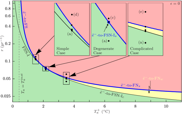
Figure 12: Singular R-tipping diagram for the reduced problem (31)–(32) with global warming scenario (30), obtained using the desingularised system (40)–(41). (Green) region of tracking, (red) region of R-tipping, and (yellow) critical range of neither tracking nor R-tipping are separated by: (blue) $\tilde{e}^{-}$-to-FS, $\tilde{e}^{-}$-to-FSN-I_s and $\tilde{e}^{-}$-to-FN_s, along which $W^{u,[r]}(\tilde{e}^{-})$ contains the singular canards $\tilde{\gamma}^{S}$, $\tilde{\gamma}^{SN}$ and $\tilde{\gamma}^{N}_{s}$, respectively, and (black) $\tilde{e}^{-}$-to-FSN-I_c, along which $W^{u,[r]}(\tilde{e}^{-})$ contains the weak folded saddle-node singular canard. See Table 1 in the electronic appendix for other parameter values.

Next, we use the singular R-tipping diagram in fig. 12 (c) together with rigorous results on persistence of singular canards as maximal canards for $0<\epsilon\ll 1$ [58, 32, 31, 66, 64] to explain the regular R-tipping diagram in fig. 8 (a).

In the simple slow case, the folded-saddle singular canard $\tilde{\gamma}^{S}$ perturbs to a family of canards when $0<\epsilon\ll 1$. The family contains one maximal canard, namely the folded-saddle maximal canard $\tilde{\gamma}^{S}_{\epsilon}$, and associated canards “without head” and “with head” [58]. Thus, these canards explain the simple part of the regular R-tipping diagram at lower values of $T_{a}^{+}$, including the (cyan) critical range and the vertical asymptote of the blue curve of maximal canards. In the context of excitable systems, we use Def. 5.3(ii) to relate a family of canards “without head” associated with a codimension-one normally hyperbolic repelling slow manifold near FS to a simple excitability quasithreshold; see also [69, 41].

In the complicated slow case, the perturbed dynamics for $0<\epsilon\ll 1$ are far less straightforward due to the presence of many folded-node maximal canards in addition to the folded-saddle maximal canard. The number and type of folded-node maximal canards depend on the distance between FN and FS, and on the ratio of the weak and strong eigenvalues of FN, denoted $\mu\in(0,1)$. The folded-node strong singular canard $\tilde{\gamma}^{N}_{s}$ perturbs to a family of canards for all $\mu\in(0,1)$. This family contains the folded-node strong maximal canard $\tilde{\gamma}^{N}_{s,\epsilon}$ and associated canards “without head” and “with head”. Depending on $\mu$, the family of folded-node weak singular canards from the singular funnel may perturb to a single folded-node weak maximal canard $\tilde{\gamma}^{N}_{w,\epsilon}$ [66, 68]. Additionally, there can be a number of secondary folded-node maximal canards that lie between $\tilde{\gamma}^{N}_{s,\epsilon}$ and $\tilde{\gamma}^{N}_{w,\epsilon}$ [58, 66, 19]. Furthermore, the folded-saddle singular faux canard perturbs to folded-saddle faux canards, which may interact with secondary folded-node maximal canards near FSN-I [40]. The interplay between the folded-node and the folded-saddle can give rise to real-faux canards described in [48, 64], that are a perturbation of the red trajectory from fig. 10 (b), and to composite canards identified in [48], that follow the folded-saddle maximal canard and then ‘switch’ to and follow one of the folded-node maximal canards. For example, we have checked that as $r$ is increased for a fixed $T_{a}^{+}\gtrsim 9.3^{\circ}$C in fig. 8 (a), $W^{u,[r]}(\tilde{e}^{-})$ coalesces with a secondary folded-node canard at the bottom boundary of the R-tipping tongue, then with a composite canard at the upper boundary of the tongue, and finally with the folded-node strong maximal canard at the bottom boundary of the main R-tipping region [44]. Thus, it is folded-node maximal canards and composite canards, together with the associated canards “without head” and “with head”, that give rise to the complicated tracking-tipping transitions including R-tipping tongue(s), at higher values of $T_{a}^{+}$. In the context of excitable systems, we use Def. 5.3(ii) to relate a family of canards “without head” associated with a codimension-one normally hyperbolic repelling slow manifold near FN to a new type of excitability quasithreshold. This quasithreshold is expected to have an intricate shape as indicated by the computations of slow manifolds in [18, 49].

7 The R-Tipping Mechanism for Summer Heatwaves

The R-tipping instability in fig. 3 arises because time-variation of the atmospheric temperature $T_{a}$ interacts with the fast timescale of soil temperature $T$. Thus, to uncover the underlying dynamical mechanisms, we consider the 2-fast 1-slow system (13)–(15) with the rate parameter $r\lesssim 1/\epsilon$, where $u=rt\lesssim\tau$ becomes another fast time and $s$ becomes another fast variable.

The singular reduced problem, obtained by setting $\epsilon=1/r=0$ for the slow time $t$ in (13)–(15),

$$\frac{dC}{dt} =f_{2}(T,C),$$ (42)

gives slow timescale solutions evolving on a critical manifold that consists of two disconnected one-dimensional components

$$S=S^{-}\cup S^{+},\quad S^{\mp} =\left\{(T,C,s)~{}:~{}f_{1}(T,C,0)=0,~{}s=\mp 1\right\}.$$ (43)

Specifically, $S^{-}=S^{-}_{1}\cup F_{1}^{-}\cup S^{-}_{2}\cup F_{2}^{-}\cup S^{-}_{3}$ is the critical manifold of the past limit system (9) with $T_{a}^{-}=0^{\circ}$C, embedded in the compactified phase space where it gains one unstable direction. Similarly, $S^{+}=S^{+}_{1}\cup F_{1}^{+}\cup S^{+}_{2}\cup F_{2}^{+}\cup S^{+}_{3}$ is the critical manifold of the future limit system (10) with $T_{a}^{+}=0^{\circ}$C, embedded in the compactified phase space where it gains one stable direction. The attracting branch $S_{3}^{+}$ is the hot metastable state; see fig. 13 (b). The layer problem, obtained by defining $r=\tilde{r}/\epsilon$ for some constant $\tilde{r}={\cal O}(1)$ and taking the limit $\epsilon\to 0$ for the fast time $\tau=t/\epsilon$,

$$\frac{dT}{d\tau} =f_{1}(T,C,T_{a}^{\nu}(s)),$$ (44)

$$\frac{ds}{d\tau} ={\frac{\tilde{r}\,\nu}{2}}\,(1-s^{2}),$$ (45)

gives fast timescale solutions on a two-dimensional layer with a fixed-in-time $C$,

$$L=\left\{(T,C,s)~{}:~{}C={\rm const.}\right\}.$$ (46)

As a model of a summer heatwave, we sacrifice seasonal variations to simplify the analysis and consider a fast impulse rising from $T_{a}^{min}=0^{\circ}$C to a given $T_{a}^{max}>0^{\circ}$C and then dropping back to $0^{\circ}$C, that decays exponentially with the decay coefficient $\rho=1$ as per definition 4.1,

$$T_{a}(rt)=T_{a}^{max}\operatorname{sech}{(rt)}.$$ (47)

We then fix the compactification parameter $\nu=1/2$ and apply the inverse of the compactification transformation (12) to (47) to obtain

$$T_{a}^{\nu}(s)=T_{a}^{\frac{1}{2}}(s)=\frac{2\,T_{a}^{max}\,(1-s)^{2}}{(1+s)^{4}+(1-s)^{4}}.$$ (48)

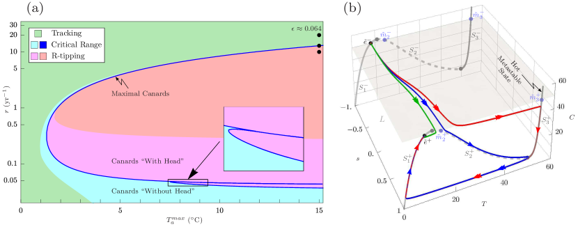
Figure 13: (a) R-tipping diagram for nonautonomous system (3)–(4) with summer heatwave (47), in the plane of the impulse amplitude $T_{a}^{max}$ and the rate parameter $r$, for $\epsilon\approx 0.064$; note the logarithmic scale for $r$. Shown are regions of (green) tracking, (cyan, blue) critical range, and (magenta, red) R-tipping from $\tilde{e}^{-}$. (b) (Colour) The unstable invariant manifold $W^{u,[r]}_{\nu}(\tilde{e}^{-})$ of the saddle $\tilde{e}^{-}$ for the compactified system (13)–(15) with $\epsilon\approx 0.064$, summer heatwave (48) with $T_{a}^{max}=15^{\circ}$C and $\nu=1/2$, and three different values of the rate parameter: (green) $r=20$, (blue) $r\approx 12.9123$, and (red) $r=10$; see the black dots in (a). Included for reference are (dark grey) the two disconnected components $S^{-}$ and $S^{+}$ of the critical manifold, (light grey) the layer $L$ defined by $C=C^{e}(0)$, and (light blue) four new equilibria $\tilde{m}_{2}^{\pm}$ and $\tilde{m}_{3}^{\pm}$ for the layer problem (44)–(45). See Table 1 in the electronic appendix for other parameter values.

To give a full overview of transitions from tracking to R-tipping for impulse inputs, and to make connections to section 6, we plot an R-tipping diagram in the plane $(T_{a}^{max},r)$ of the input parameters in fig. 13 (a) for a wide range of the rate parameter $r$. The diagram was obtained by computing $W^{u,[r]}(\tilde{e}^{-})$ in system (13)–(15) with $0<\epsilon\ll 1$ for different values of $T_{a}^{max}$ and $r$, and using Defs. 5.1–5.3 to identify different dynamical regions for system (3)–(4). The families of canards were considered relative to the evolving slow manifold, from two-dimensional $S$ in (27) to one dimensional $S^{+}$ in (43), as $r$ was increased. The shape of the R-tipping region in fig. 13 (a) is rather different to that obtained in fig. 8 (a). There are two R-tipping tongues, one large akin to that in [43, Sec.6] and one small akin to that in fig. 8 (a), each enclosing a separate (magenta, red) region of R-tipping. The lower part of the diagram corresponds to slow impulses that last for decades (1-fast 2-slow system). The tracking-tipping transitions in this part occur during the rise of the impulse $T_{a}(rt)$, and are of the same type as those described in section 6. The upper part of the diagram corresponds to fast impulses (2-fast 1-slow system) and is the focus of this section. The rate parameter $r$ in the range of 10 to 15 yr^-1 gives a pulse duration in the range of 3 to 2 months, in line with realistic summer heatwaves [47]. Thus, the single tipping-tracking transition found in the upper part of the diagram quantifies the intensity and duration of summer heatwaves that trigger R-tipping to the hot metastable state in the soil-carbon system (3)–(4).

To gain geometric insight into the R-tipping instability caused by a summer heatwave, we plot in fig. 13 (b) the unstable manifold $W^{u,[r]}(\tilde{e}^{-})$ for a fixed $T_{a}^{+}=15^{\circ}$C and three different fast rates $r_{1}>r_{2}>r_{3}>0$ (see the black dots in fig. 13 (a)), together with the (light gray) layer $L$ of constant $C=C^{e}(0)$ and the (dark gray) critical manifold $S=S^{-}\cup S^{+}$. Figure 13 (b) shows that, as $r$ is decreased (the duration of the heatwave is increased), tracking by (green) $W^{u,[r_{1}]}(\tilde{e}^{-})$ is lost via canard trajectories, including the maximal canard contained in (blue) $W^{u,[r_{2}]}(\tilde{e}^{-})$ that approaches $S_{2}^{+}$ and moves along $S_{2}^{+}$ for the longest time. This is followed by R-tipping at lower $r$ as shown by (red) $W^{u,[r_{3}]}(\tilde{e}^{-})$ that visits the hot metastable state $S^{+}_{3,\epsilon}$ before connecting to $\tilde{e}^{+}\in S^{+}_{1,\epsilon}$. Since tracking-tipping transitions due to a summer heatwave (47) occur when the fast timescale segment of $W^{u,[r]}(\tilde{e}^{-})$ on $L$ approaches the hyperbolic saddle branch $S_{2}^{+}$ of $S^{+}$, it should be possible to explain the upper part of the R-tipping diagram in fig. 13 in terms of fast timescale solutions of a suitably chosen two-dimensional layer problem alone.

7.1 One Fast Case in the Layer Problem

The suitable layer problem for the 2-fast 1-slow system (13)–(15) with a summer heatwave (48) is obtained by fixing $C$ in (44)–(45) and (46) at the equilibrium soil-carbon concentration $C^{e}(0)$ for the past and future limit systems. Crucially, such a layer problem (44)–(45) has six equilibria. Two of these equilibria, namely the saddle $\tilde{e}^{-}\in S^{-}_{1}$ and the base-state sink $\tilde{e}^{+}\in S^{+}_{1}$, are the equilibria of the compactified system (13)–(15). The four new equilibria, that do not exist in (13)–(15), are found at the intersections of $L$ with $S^{\pm}_{2,3}$. These are: the source $\tilde{m}^{-}_{2}\in S_{2}^{-}$, the saddle $\tilde{m}^{-}_{3}\in S_{3}^{-}$, the saddle $\tilde{m}^{+}_{2}\in S_{2}^{+}$, and the hot-state sink $\tilde{m}^{+}_{3}\in S_{3}^{+}$; see the (blue) dots in fig. 13 (b).

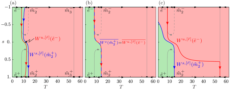
Figure 14: The fast case of tracking-tipping transition in phase portraits of the layer problem (44)–(45) with $C=C^{e}(0)$ and $\nu=1/10$. Note tracking in (a), and loss of tracking via a codimension-one heteroclinic orbit connecting $\tilde{e}^{-}$ to $\tilde{m}_{2}^{+}$ in (b) that leads to R-tipping in (c). $T_{a}^{+}=15$ and the rate parameter takes values $(a)\ \tilde{r}=1.28$, $(b)\ \tilde{r}=\tilde{r}_{c}\approx 0.972269$, and $(c)\ \tilde{r}=0.64$; see the black dots in the inset of fig. 15. Included for reference are different branches of (grey) $\tilde{M}$. See the electronic appendix for other parameter values in Table 1 and for definition of $\tilde{M}$ in section 6.

To be precise and consistent with Defs. 5.2 and 5.3 for $0<\epsilon\ll 1$, we now define tracking, R-tipping and critical rates for fast external inputs in the limit $\epsilon=0$ as follows:

Definition 7.1.

In the layer problem (44)–(45), we say that,

• Tracking occurs when $W^{u,[{\tilde{r}}]}(\tilde{e}^{-})$ connects to the base-state sink $\tilde{e}^{+}$.

• R-tipping occurs when $W^{u,[{\tilde{r}}]}(\tilde{e}^{-})$ connects to the hot-state sink $\tilde{m}_{3}^{+}$.

• A critical rate is an isolated value of ${\tilde{r}}$ that gives neither tracking nor R-tipping.

In other words, in the the layer problem (44)–(45), the question of loss of tracking boils down to whether or not $W^{u,[{\tilde{r}}]}(\tilde{e}^{-})$ connects to the saddle $\tilde{m}_{2}^{+}$. Thus, the saddle $\tilde{m}_{2}^{+}$ is another example of the “singular R-tipping edge state” described in the introduction.

The dynamics of the layer problem (44)–(45) on $L$ are shown in a series of phase portraits in fig. 14, where we fix $T_{a}^{max}=15>T_{a}^{inst}$ and decrease $\tilde{r}$ across the critical rate. The basin of attraction of $\tilde{e}^{+}$ is plotted in green, and the basin of attraction of $\tilde{m}_{3}^{+}$ is plotted in dark red. The rate-dependent (blue) stable manifold of $\tilde{m}_{2}^{+}$, denoted $W^{s,[{\tilde{r}}]}(\tilde{m}_{2}^{+})$, is contained in the basin boundary separating these two basins of attraction. For ${\tilde{r}}$ sufficiently large, (red) $W^{u,[{\tilde{r}}]}(\tilde{e}^{-})$ lies in the basin of attraction of $\tilde{e}^{+}$ and connects to $\tilde{e}^{+}$; see fig. 14 (a). When ${\tilde{r}=\tilde{r}_{c}}$, $W^{u,[{\tilde{r}}]}(\tilde{e}^{-})$ coalesces with $W^{s,[{\tilde{r}}]}(\tilde{m}_{2}^{+})$ along the basin boundary. At this point, tracking is lost since $W^{u,[{\tilde{r}}]}(\tilde{e}^{-})$ connects to the saddle $\tilde{m}_{2}^{+}$; see fig. 14 (b). For ${\tilde{r}<\tilde{r}_{c}}$, $W^{u,[{\tilde{r}}]}(\tilde{e}^{-})$ lies in the basin of attraction of $\tilde{m}_{3}^{+}$ and connects to $\tilde{m}_{3}^{+}$. In other words, R-tipping occurs for $r<r_{c}$; see fig. 14 (c).

Thus, in the layer problem (44)–(45) with $C=C^{e}(0)$, there is just one case of a tracking-tipping transition, where tracking is lost at a critical rate ${\tilde{r}=\tilde{r}}_{c}$. We refer to this case as the fast case to distinguish it from the three slow cases identified in section 66.2. The critical rate is the value of $r$ that gives a codimension-one hetroclinic orbit connecting $\tilde{e}^{-}$ to the new saddle $\tilde{m}_{2}^{+}$ for the layer problem (44)–(45). For additional insight into R-tipping caused by a summer heatwave, we refer to section 6 of the electronic appendix.

7.2 Bringing it Together: Additional Saddle-to-Saddle Heteroclinic Orbit

In this section, we first produce the singular R-tipping diagram for $\epsilon=0$ in fig. 15, and then use it to explain the regular R-tipping diagram for $\epsilon\approx 0.064$ in fig. 13 (a).

In the singular R-tipping diagram in fig. 15, the lower-$r$ tracking-tipping transitions were obtained in the same manner as outlined in section 6, that is by computing different heteroclinic orbits in the desingularised system for the slow impulse $T_{a}^{1/2}(s)$ in (48). To avoid repetition, we skip the derivations and refer to sections 66.2 and 66.3 for more details.

The higher-${\tilde{r}}$ tipping-tracking transition, which is the focus of this section, is given by the (blue) curve denoted $\tilde{e}^{-}$-to-$\tilde{m}_{2}^{+}$. This curve was obtained by computing a codimension-one heteroclinic orbit connecting the saddle $\tilde{e}^{-}$ to the saddle $\tilde{m}_{2}^{+}$ in the layer problem (44)–(45); see fig. 14 (b). This heteroclinic connection gives the critical rate when $\overline{W^{u,[{\tilde{r}}]}(\tilde{e}^{-})}=\overline{W^{s,[{\tilde{r}}]}(\tilde{m}_{2}^{+})}$ , and is the only case of loss of tracking for (44)–(45). Note that curves $\tilde{e}^{-}$-to-$\tilde{m}_{2}^{+}$ and $\tilde{e}^{-}$-to-FS have a common vertical asymptote $T_{a}^{max}=T_{a}^{inst}\approx 0.423364$, which is given by condition (24) illustrated in fig. 7.

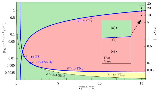
Figure 15: Singular R-tipping diagram obtained using a combination of two problems. (The upper curve $\tilde{e}^{-}$-to-$\tilde{m}^{+}_{2}$) the two-dimensional layer problem (44)–(45) with summer heatwave (48), rate parameter $\tilde{r}=\epsilon r$ shown on the left vertical axis, and $\nu=1/2$. (The lower curves) the two-dimensional reduced problem (31)–(32) with slow impulse (48) and rate paraemeter $r$ shown on the right vertical axis. Note the logarithmic scales for $r$ and $\tilde{r}$. At higher ${\tilde{r}}$, the (red) region of R-tipping is separated from the (green) region of tracking by the (blue) curve $\tilde{e}^{-}$-to-$\tilde{m}^{+}_{2}$, along which $W^{u,[{\tilde{r}}]}(\tilde{e}^{-})$ intersects $W^{s,[{\tilde{r}}]}(\tilde{m}^{+}_{2})$ in (44)–(45). For lower $r$, see the caption of fig. 12 (c). See Table 1 in the electronic appendix for other parameter values.

Next, in addition to the ‘first’ Fenichel theorem on persistence of normally hyperbolic critical manifolds as slow manifolds for $0<\epsilon\ll 1$, we recall the ‘second’ Fenichel theorem that guarantees persistence of stable and unstable invariant manifolds of normally hyperbolic saddle critical manifolds when $0<\epsilon\ll 1$ [22, 23, 27, 68, 34]. We then use the singular R-tipping diagram in fig. 15, together with both Fenichel theorems and rigorous results on persistence of singular canards as maximal canards for $0<\epsilon\ll 1$ [58, 32, 31, 64, 66], to explain the regular R-tipping diagram in fig. 13 (a).

In the fast case, the heteroclinic $\tilde{e}^{-}$-to-$\tilde{m}_{2}^{+}$ connection for the layer problem (44)–(45) perturbs to an intersection of $W^{u,[{\tilde{r}}]}(\tilde{e}^{-})$ with the (fast) stable manifold of the normally hyperbolic saddle slow manifold $S_{2,\epsilon}^{+}$ in the compactified system (13), giving rise to the (blue) maximal canard shown in fig. 13 (b). In other words, $W^{u,[{\tilde{r}}]}(\tilde{e}^{-})$ approaches the normally hyperbolic saddle slow manifold $S^{+}_{2,\epsilon}$ along its stable manifold, thus moves along $S^{+}_{2,\epsilon}$ for as long $S^{+}_{2,\epsilon}$ exists, then approaches the stable slow manifold $S^{+}_{1,\epsilon}$ and eventually connects to $\tilde{e}^{+}$. In addition, for nearby values of $r$, we expect associated canards “without head” and canards“with head”. These occur when $W^{u,[{\tilde{r}}]}(\tilde{e}^{-})$ near misses the stable manifold of $S_{2,\epsilon}^{+}$ to the left or right, respectively, and diverges away from $S_{2,\epsilon}^{+}$ before $S_{2,\epsilon}^{+}$ ceases to exist. Thus, it is the (blue) maximal canard shown in fig. 13 (b), together with the associated canards “without head”, that give rise to the higher-$r$ tipping-tracking transition in the regular R-tipping diagram in fig. 13 (a). In the context of excitable systems, we use Def. 5.3(ii) to relate a family of canards “without head” associated with a codimension-one stable manifold of a normally hyperbolic saddle slow manifold to yet another new type of excitability quasithreshold.

8 Conclusion and Outlook

In this paper, we obtain two kinds of results. First, we demonstrate that sufficiently fast atmospheric warming can cause R-tipping to a subsurface hot metastable state in bioactive peat soils, using a conceptual process-based ODE model with realistic soil parameter values and contemporary climate patterns. This gives rise to the hypothesis that such R-tipping is a main cause of “Zombie fires” observed in peatlands, that disappear from the surface, smoulder underground during the winter, and “come back to life” in the spring. Second, we recognise that such R-tipping is a nonautonomous instability that occurs due to crossing an elusive quasithreshold in the phase space of a multiple-timescale dynamical system, and thus cannot be explained by traditional autonomous stability theory. Therefore, to understand the underlying dynamical mechanisms, we provide a mathematical framework that is underpinned by a compactification technique for asymptotically autonomous dynamical systems and concepts from geometric singular perturbation theory, such as slow manifolds, canard trajectories and folded singularities. This framework explains R-tipping to the hot metastable state in the soil-carbon system and, more generally, identifies generic cases of tracking-tipping transitions due to crossing a quasithreshold. Furthermore, we show that a quasithreshold gives rise to critical ranges of the rate of change of the external input rather than isolated critical rates, and reveal new types of quasithresholds. These results pose two types of challenges for future research.

First, to strengthen our hypothesis, it would be interesting to build on the excellent agreement with the medium-complexity PDE model in fig. 5 and extend the conceptual ODE model in different directions. For example, include terms describing peat soil ignition processes at higher temperatures [74]. This would allow investigation of existence of additional (quasi)thresholds for the onset of flames. Include other physical processes, in addition to soil temperature, that contribute to microbial soil respiration. For example, the inclusion of soil hydrology would extend the applicability of the model; see for example DigiBog_Hydro [7] and [65]. Include random fluctuations to account for the fact that climate and weather patterns are inherently noisy. This would give a more accurate description of the tipping being a combination of R-tipping and noise-induced tipping (N-tipping). Understanding how the two tipping mechanisms interact is non-trivial [50, 57] and an area of ongoing research for quasithresholds. Account for spatio-temporal dynamics by extending the conceptual ODE model to a PDE model. Vertical diffusion has already been studied in the extended Luke and Cox model with interesting results confirming validity of the conceptual ODE model [17]. Finally, it might be interesting to couple the conceptual model to spatially extended land-surface models such as JULES [6] or DigiBog [5]. Currently, such models often neglect heat produced by microbial decomposition which is a key factor for the R-tipping instability to the hot metastable state described in this paper.

Second, there are challenges related to extending the mathematical framework and obtaining rigorous results. One is the extension of the compactification technique to asymptotically periodic inputs and usage of geometrical singular perturbation theory to analyse external inputs with seasonal variations. Another is a general theory of R-tipping due to crossing quasithresholds in multiple-timescale systems, for which the definitions of R-tipping and a quasithreshold introduced here for the soil-carbon system are a good starting point. Of particular interest to scientists and mathematical modelers are rigorous yet easily testable criteria for the occurrence of such R-tipping, akin to those derived in [70] for R-tipping due to crossing regular thresholds.

References

- [1] 2021 2021 38℃ record Arctic temperature confirmed, others likely to follow: WMO. UN News, 14 December. See https://news.un.org/en/story/2021/12/1107872.
- [2] 2021 Chersky climate: Average Temperature, weather by month. Climate-Data.org. See https://en.climate-data.org/asia/russian-federation/sakha-republic/chersky-333972/#climate-table. Accessed: 2021-04-21.
- [3] 2021 What are ’zombie fires’ and why is the Arctic Circle on fire?. BBC Newsround, 20 May. See https://www.bbc.co.uk/newsround/57173570.
- [4] 2022 Berkeley Earth: Data Overview. See http://berkeleyearth.org/data/.
- [5] 2022 Digibog: water@leeds. See https://water.leeds.ac.uk/our-missions/mission-1/digibog/. Accessed: 2022-09-12.
- [6] 2022 Joint UK Land Environment Simulator (JULES). See https://jules.jchmr.org/. Accessed: 2022-09-12.
- [7] 2022 Resources: water@leeds. See https://water.leeds.ac.uk/our-missions/mission-1/digibog/resources/. Accessed: 2022-09-12.
- [8] Ashwin P, Wieczorek S, Vitolo R, Cox P. 2012 Tipping points in open systems: bifurcation, noise-induced and rate-dependent examples in the climate system. Phil. Trans. R. Soc. A 370, 1166–1184.
- [9] Ashwin P, Perryman C, Wieczorek S. 2017 Parameter shifts for nonautonomous systems in low dimension: bifurcation- and rate-induced tipping. Nonlinearity 30, 2185–2210.
- [10] Benoît É. 1983 Systemes lents-rapides dans R3 et leurs canards. Asterisque pp. 109–110.
- [11] Benoît É, Callot J, Diener F, Diener M. 1981 Chasse au canard (première partie). Collectanea Mathematica 32, 37–76.
- [12] Boers N, Rypdal M. 2021 Critical slowing down suggests that the western Greenland Ice Sheet is close to a tipping point. Proc. Natl Acad. Sci. 118, e2024192118.
- [13] Buggeln R, Rynk R. 2002 Self-Heating In Yard Trimmings: Conditions Leading To Spontaneous Combustion. Compost Science & Utilization 10, 162–182.
- [14] Caesar L, Rahmstorf S, Robinson A, Feulner G, Saba V. 2018 Observed fingerprint of a weakening Atlantic Ocean Overturning Circulation. Nature 556, 191–196.
- [15] Cardin PT, Teixeira MA. 2017 Fenichel theory for multiple time scale singular perturbation problems. SIAM Journal on Applied Dynamical Systems 16, 1425–1452.
- [16] Chow S, Lin X. 1990 Bifurcation of a homoclinic orbit with a saddle-node equilibrium. Differential and Integral Equations 3, 435–466.
- [17] Clarke J, Huntingford C, Ritchie P, Cox P. 2021 The compost bomb instability in the continuum limit. Eur. Phys. J. Spec. Top. 230, 3335–3341.
- [18] Desroches M, Krauskopf B, Osinga HM. 2008 The geometry of slow manifolds near a folded node. SIAM J. Appl. Dyn. Syst. 7, 1131–1162.
- [19] Desroches M, Krauskopf B, Osinga HM. 2010 Numerical continuation of canard orbits in slow–fast dynamical systems. Nonlinearity 23, 739–765.
- [20] Dumortier F, Roussarie R. 1996 Canard Cycles and Center Manifolds. Number no. 577 in American Mathematical Society: Memoirs of the American Mathematical Society. American Mathematical Soc.
- [21] Dumortier F. 1993 Techniques in the Theory of Local Bifurcations: Blow-Up, Normal Forms, Nilpotent Bifurcations, Singular Perturbations. In Schlomiuk D, editor, Bifurcations and Periodic Orbits of Vector Fields pp. 19–73. Dordrecht: Springer Netherlands.
- [22] Fenichel N, Moser JK. 1971 Persistence and Smoothness of Invariant Manifolds for Flows. Indiana University Mathematics Journal 21, 193–226.
- [23] Fenichel N. 1979 Geometric Singular Perturbation Theory for Ordinary Differential Equations. Journal of Differential Equations 31, 53–98.
- [24] FitzHugh R. 1955 Mathematical models of threshold phenomena in the nerve membrane. The bulletin of mathematical biophysics 17, 257–278.
- [25] Hastings A, Abbott KC, Cuddington K, Francis T, Gellner G, Lai YC, Morozov A, Petrovskii S, Scranton K, Zeeman ML. 2018 Transient phenomena in ecology. Science 361, eaat6412.
- [26] Izhikevich EM. 2006 Dynamical systems in neuroscience: the geometry of excitability and bursting. Cambridge, MA: The MIT Press.
- [27] Jones CKRT. 1995 Geometric Singular Perturbation Theory. In Johnson R, editor, Dynamical Systems. Lecture Notes in Mathematics. Berlin, Heidelberg: Springer.
- [28] Khvorostyanov DV, Ciais P, Krinner G, Zimov SA, Corradi C, Guggenberger G. 2008a Vulnerability of permafrost carbon to global warming. Part II: sensitivity of permafrost carbon stock to global warming. Tellus B: Chemical and Physical Meteorology 60, 265–275.
- [29] Khvorostyanov DV, Krinner G, Ciais P, Heimann M, Zimov SA. 2008b Vulnerability of permafrost carbon to global warming. Part I: model description and role of heat generated by organic matter decomposition. Tellus B 60, 250–264.
- [30] Kirschbaum MUF. 1995 The temperature dependence of soil organic matter decomposition, and the effect of global warming on soil organic C storage. Soil Biology and Biochemistry 27, 753–760.
- [31] Krupa M, Szmolyan P. 2001 Extending Geometric Singular Perturbation Theory to Nonhyperbolic Points—Fold and Canard Points in Two Dimensions. SIAM J. Math. Anal 33, 286–314.
- [32] Krupa M, Wechselberger M. 2010 Local analysis near a folded saddle-node singularity. Journal of Differential Equations 248, 2841–2888.
- [33] Kuehn C. 2011 A mathematical framework for critical transitions: Bifurcations, fast–slow systems and stochastic dynamics. Physica D 240, 1020–1035.
- [34] Kuehn C. 2016 Multiple Time Scale Dynamics. Springer International PU.
- [35] Lenton TM, Held H, Kriegler E, Hall JW, Lucht W, Rahmstorf S, Schellnhuber HJ. 2008 Tipping elements in the Earth’s climate system. Proc. Natl Acad. Sci. 105, 1786–1793.
- [36] Luke CM, Cox PM. 2011 Soil carbon and climate change: from the Jenkinson effect to the compost-bomb instability. European Journal of Soil Science 62, 5–12.
- [37] Masson-Delmotte V, Zhai P, Pörtner HO, Roberts D, Skea J, Shukla P, Pirani A, Moufouma-Okia W, Péan C, Pidcock R, Connors S, Matthews J, Chen Y, Zhou X, Gomis M, Lonnoy E, Maycock T, Tignor M, Waterfield Te. 2018 Global Warming of 1.5°C. An IPCC Special Report on the impacts of global warming of 1.5°C above pre-industrial levels and related global greenhouse gas emission pathways, in the context of strengthening the global response to the threat of climate change, sustainable development, and efforts to eradicate poverty.. IPCC.
- [38] Masson-Delmotte V, Zhai P, Pirani A, Connors SL, Péan C, Berger S, Caud N, Chen Y, Goldfarb L, Gomis M et al.. 2021 Climate change 2021: the physical science basis. Contribution of working group I to the sixth assessment report of the intergovernmental panel on climate change 2.
- [39] McCarty JL, Smith TEL, Turetsky MR. 2020 Arctic fires re-emerging. Nature Geoscience 13, 658–660.
- [40] Mitry J, Wechselberger M. 2017 Folded Saddles and Faux Canards. SIAM Journal on Applied Dynamical Systems 16, 546–596.
- [41] Mitry J, McCarthy M, Kopell N, Wechselberger M. 2013 Excitable neurons, firing threshold manifolds and canards. Journal of Mathematical Neuroscience 3, 12.
- [42] Mäkiranta P, Laiho R, Fritze H, Hytönen J, Laine J, Minkkinen K. 2009 Indirect regulation of heterotrophic peat soil respiration by water level via microbial community structure and temperature sensitivity. Soil Biology and Biochemistry 41, 695–703.
- [43] O’Keeffe PE, Wieczorek S. 2020 Tipping Phenomena and Points of No Return in Ecosystems: Beyond Classical Bifurcations. SIAM J. Appl. Dyn. Syst. 19, 2371–2402. Publisher: Society for Industrial and Applied Mathematics.
- [44] O’Sullivan E. 2023 Rate-Induced Tipping to Metastable Zombie Fires. PhD thesis University College Cork.
- [45] Overland J, Dunlea E, Box JE, Corell R, Forsius M, Kattsov V, Olsen MS, Pawlak J, Reiersen L, Wang M. 2019 The urgency of Arctic change. Polar Science 21, 6–13.
- [46] Pachauri RK, Allen MR, Barros VR, Broome J, Cramer W, Christ R, Church JA, Clarke L, Dahe Q, Dasgupta P et al.. 2014 In Climate change 2014: synthesis report. Contribution of Working Groups I, II and III to the fifth assessment report of the Intergovernmental Panel on Climate Change,. Ipcc.
- [47] Perkins-Kirkpatrick SE, Lewis SC. 2020 Increasing trends in regional heatwaves. Nat. Commun. 11.
- [48] Perryman C, Wieczorek S. 2014 Adapting to a changing environment: non-obvious thresholds in multi-scale systems. Proc. R. Soc. A 470, 20140226. Publisher: Royal Society.
- [49] Perryman CG. 2015 How fast is too fast? Rate-induced bifurcations in multiple time-scale systems. PhD thesis University of Exeter.
- [50] Ritchie P, Sieber J. 2017 Probability of noise- and rate-induced tipping. Phys. Rev. E 95, 052209.
- [51] Ritchie PD, Clarke JJ, Cox PM, Huntingford C. 2021 Overshooting tipping point thresholds in a changing climate. Nature 592, 517–523.
- [52] Rohde R, Muller R, Jacobsen R, Perlmutter S, Mosher S. 2013 Berkeley Earth temperature averaging process. Geoinformatics I& Geostatistics: An Overview 01.
- [53] Roy J, Saugier B, Mooney HA. 2001 Terrestrial Global Productivity. Elsevier.
- [54] Sawer P. 2022 Wennington Fire: Compost blaze that devastated village started just yards from fire station. The Telegraph, 20 July. See https://www.telegraph.co.uk/news/2022/07/20/wennington-fire-compost-blaze-devastated-village-started-just/.
- [55] Scholten RC, Jandt R, Miller EA, Rogers BM, Veraverbeke S. 2021 Overwintering fires in boreal forests. Nature 593, 399–404.
- [56] Screen JA, Simmonds I. 2010 The central role of diminishing sea ice in recent Arctic temperature amplification. Nature 464, 1334–1337.
- [57] Slyman K, Jones CK. 2022 Rate and Noise-Induced Tipping Working in Concert. arXiv.
- [58] Szmolyan P, Wechselberger M. 2001 Canards in R3. J. Differ. Equ. 177, 419–453.
- [59] Tarnocai C, Canadell JG, Schuur EaG, Kuhry P, Mazhitova G, Zimov S. 2009 Soil organic carbon pools in the northern circumpolar permafrost region. Global Biogeochemical Cycles 23.
- [60] Thompson JM, Sieber J. 2011 Predicting climate tipping as a noisy bifurcation: A Review. International Journal of Bifurcation and Chaos 21, 399–423.
- [61] UNFCCC V. 2015 Adoption of the Paris agreement vol. 282. Proposal by the President.
- [62] Vanselow A, Wieczorek S, Feudel U. 2019 When very slow is too fast - collapse of a predator-prey system. J. Theor. Biol. 479, 64–72.
- [63] Vaughan A. 2020 Arctic ‘zombie fires’ keep burning beneath the ice. New Scientist 246, 14.
- [64] Vo T, Wechselberger M. 2015 Canards of Folded Saddle-Node Type I. SIAM J. Math. Anal 47, 3235–3283.
- [65] Waddington JM, Morris PJ, Kettridge N, Granath G, Thompson DK, Moore PA. 2014 Hydrological feedbacks in northern peatlands. Ecohydrology 8, 113–127.
- [66] Wechselberger M. 2005 Existence and Bifurcation of Canards in in the Case of a Folded Node. SIAM J. Appl. Dyn. Syst. 4, 101–139.
- [67] Wechselberger M. 2007 Canards. Scholarpedia 2, 1356. revision #152256.
- [68] Wechselberger M, Mitry J, Rinzel J. 2013 Canard Theory and Excitability. In Kloeden PE, Pötzsche C, editors, Nonautonomous Dynamical Systems in the Life Sciences pp. 89–132. Cham: Springer International Publishing.
- [69] Wieczorek S, Ashwin P, Luke CM, Cox PM. 2011 Excitability in ramped systems: the compost-bomb instability. Proc. R. Soc. A 467, 1243–1269.
- [70] Wieczorek S, Xie C, Ashwin P. 2021a Rate-induced tipping: Thresholds, edge states and connecting orbits. arXiv preprint arXiv:2111.15497.
- [71] Wieczorek S, Xie C, Jones CKRT. 2021b Compactification for asymptotically autonomous dynamical systems: theory, applications and invariant manifolds. Nonlinearity 34, 2970–3000.
- [72] Xu J, Morris PJ, Liu J, Holden J. 2018 PEATMAP: Refining estimates of global peatland distribution based on a meta-analysis. CATENA 160, 134–140.
- [73] Yu ZC. 2012 Northern peatland carbon stocks and dynamics: a review. Biogeosciences 9, 4071–4085.
- [74] Yuan H, Restuccia F, Rein G. 2021 Spontaneous ignition of soils: A multi-step reaction scheme to simulate self-heating ignition of smouldering peat fires. Int. J. Wildland Fire 30, 440.
- [75] Zimov SA, Schuur EA, Chapin III FS. 2006 Permafrost and the global carbon budget. Science 312, 1612–1613.