Dynamics of dwarf galaxies in $f(R)$ gravity

Abstract

We use the kinematic data of the stars in eight dwarf spheroidal galaxies to assess whether $f(R)$ gravity can fit the observed profiles of the line-of-sight velocity dispersion of these systems without resorting to dark matter. Our model assumes that each galaxy is spherically symmetric and has a constant velocity anisotropy parameter $\beta$ and constant mass-to-light ratio consistent with stellar population synthesis models. We solve the spherical Jeans equation that includes the Yukawa-like gravitational potential appearing in the weak field limit of $f(R)$ gravity, and a Plummer density profile for the stellar distribution. The $f(R)$ velocity dispersion profiles depends on two parameters: the scale length $\xi^{-1}$, below which the Yukawa term is negligible, and the boost of the gravitational field $\delta>-1$. $\delta$ and $\xi$ are not universal parameters, but their variation within the same class of objects is expected to be limited. The $f(R)$ velocity dispersion profiles fit the data with a value $\xi^{-1}=1.2^{+18.6}_{-0.9}$ Mpc for the entire galaxy sample. On the contrary, the values of $\delta$ show a bimodal distribution that picks at $\overline{\delta}=-0.986\pm 0.002$ and $\overline{\delta}=-0.92\pm 0.01$. These two values disagree at $6\sigma$ and suggest a severe tension for $f(R)$ gravity. It remains to be seen whether an improved model of the dwarf galaxies or additional constraints provided by the proper motions of stars measured by future astrometric space missions can return consistent $\delta$’s for the entire sample and remove this tension.

1 Introduction

The $\Lambda$ Cold Dark Matter ($\Lambda$CDM) model provides a theoretical framework capable of explaining the formation and evolution of cosmic structures (Planck Collaboration et al., 2020a, b, c). A few tensions remain, however, including the fine tuning problem of the cosmological constant (Weinberg, 1987, 1989; Capolupo, 2017) or the tension on the Hubble constant (Di Valentino et al., 2021).

On the scale of galaxies, the $\Lambda$CDM model also suffers from some tensions, for example (i) the cusp/core problem, the discrepancy between the predicted steep mass density profile in the central regions of dark matter halos, and the core suggested by the observations of low surface brightness galaxies and dwarf galaxies; (ii) the missing satellite problem, the discrepancy between the predicted large number of dark matter sub-halos within the dark matter halo of a Milky Way-like galaxy and the observed small number of Milky Way satellites; and (iii) the too-big-to-fail problem, the predicted existence of bright massive satellites that remain unobserved (for comprehensive reviews see, e.g., Boylan-Kolchin et al. 2011; Bullock & Boylan-Kolchin 2017; Del Popolo & Le Delliou 2017; De Martino et al. 2020; Salucci et al. 2021).

Baryonic feedback has been invoked as a possible solution to these challenges on the scale of galaxies; however, the details of the role and efficiency of baryonic feedback remain debated (e.g., De Martino et al., 2020), and it might thus not provide the full solution. Indeed, these challenges may also point out to a breakdown of the standard law of gravity, General Relativity (GR) and its Newtonian weak-field limit (De Martino et al., 2020). The $f(R)$ theories are among the simplest and most studied extensions of GR. In these theories, the Einstein-Hilbert Lagrangian is replaced by a more generic function, $f(R)$, of the Ricci scalar, $R$. These theories give rise to fourth-order field equations where the additional degrees of freedom can be recast as an effective dark energy fluid. We can thus explain the accelerated expansion of the Universe without resorting to an exotic, and yet to be understood, dark component (see for instance Starobinsky 1980; Li & Barrow 2007; Nojiri & Odintsov 2007; Starobinsky 2007; Hu & Sawicki 2007; Amendola & Tsujikawa 2008; Cognola et al. 2008; Miranda et al. 2009; Nojiri & Odintsov 2011; De Martino et al. 2015; Nojiri et al. 2017; Lazkoz et al. 2018, and references therein).

A $f(R)$ gravity theory can also mimic the dark matter component required to describe the dynamics of cosmic structure in standard gravity (Capozziello & De Laurentis, 2012). When we assume a Taylor expandable $f(R)$ Lagrangian, $f(R)$ gravity gives rise to two effects in the weak-field limit of a spherically symmetric metric: (1) a boost of the intensity of the gravitational field quantified by the parameter $\delta$ (the smaller is $\delta$ in the range $-1<\delta<0$, the larger is the intensity of the field compared to GR); and (2) a Yukawa-like correction to the Newtonian gravitational potential, which becomes relevant on length scales larger than $\xi^{-1}$ (Capozziello & De Laurentis, 2012; Banerjee et al., 2017). For each astrophysical system described by a local curvature $R$, $\delta$ and $\xi$ are linked to the coefficients of the Taylor expansion of $f(R)$ around a value $R_{0}$ corresponding to the curvature of the local background. For a Minkowski background $R_{0}=0$, we have $\delta=1+f^{\prime}_{0}$ and $\xi=(f^{\prime}_{0}/6f^{\prime\prime}_{0})^{1/2}$, where $f^{\prime}_{0}$ and $f^{\prime\prime}_{0}$ are the first two non-null coefficients of the Taylor expansion. We recover GR and the weak-field Newtonian limit when $\delta=0$ and $\xi\to\infty$, so that $f(R)=R$. At the scales of stellar systems, thanks to the Chameleon mechanism (Khoury & Weltman, 2004), the Yukawa deviations from the Newtonian potential leave unaltered the consistency of the observations with the classical tests of GR (Capozziello & Tsujikawa, 2008). On the other hand, at galactic and extra-galactic scales, the Chameleon mechanism is less effective due to the lower density of the environment and $\delta$ and $\xi$ can thus assume other values (Capozziello et al., 2007). Therefore, $\delta$ and $\xi$ are not universal parameters and we might expect that they assume different values in different systems, although in objects within the same class, e.g. dwarf galaxies or stellar systems, the variation should be limited.

The effectiveness of this $f(R)$ model at mimicking the dark matter component of the standard model was extensively explored on different scales, where we can assume $R_{0}=0$. On the galaxy and galaxy cluster scales, where the dynamical role of the dark matter is dominant in the standard model, the estimated value of $\delta$ is close to $-1$, as expected. For example, Napolitano et al. (2012) investigated the stellar kinematics of elliptical galaxies: they used long-slit data and planetary nebulae data out to seven times the effective radius of three elliptical galaxies to fit the velocity dispersion profiles and found $\delta$ in the range $[-0.88,-0.75]$. Similarly, Capozziello et al. (2009) found $\delta$ in the range $[-0.95,-0.85]$ by modelling the mass profile of 12 X-ray galaxy clusters. De Martino et al. (2014) found $\delta$ in the range $[-1,-0.43]$ by modeling, under the assumption of hydrostatic equilibrium, the gravitational potential well of about 600 X-ray galaxy clusters from the stacked Sunyaev-Zel’dovich (SZ) profiles from the Planck maps of the temperature anisotropies (Planck Collaboration et al., 2014). De Martino (2016) derived $\delta=-0.48\pm 0.22$ from the SZ profile of the Coma cluster. These two latter results showed the capability of the $\delta$ boosting of the gravitational field intensity to also explain the SZ emission without resorting to dark matter. On the galaxy and galaxy-cluster scales, $\xi^{-1}\sim 1$ Mpc, which is consistent with the lack of evidence, on smaller scales, of the existence of a fifth force and of the effects of the accelerated expansion of the Universe.

The Yukawa correction to the Newtonian potential was also tested on the scales of stellar systems, where dark matter is not relevant in the standard model and, in $f(R)$, $\delta$ is expected to be close to $0$, thanks to the effectiveness of the Chamaleon mechanism. De Laurentis & De Martino (2013) set $\delta=0$ and, by using the first time derivative of the orbital period of binary pulsars, showed that the second derivative of the $f(R)$ Lagrangian computed on the background must be compatible with zero with a precision $\sim 0.08$. Additionally, De Martino et al. (2018) and De Laurentis et al. (2018) described the effect of the Yukawa-term of the orbital motion of stars around a massive object. Their modelling led to a narrowing of the viable volume of the parameter space of the Yukawa potential on these scales; they found $\delta=-0.01_{-0.14}^{+0.61}$ and set a lower limit on the scale length $\xi^{-1}>6000$ AU (De Martino et al., 2021).

Here, we extend the above analyses of $\delta$ and $\xi$ by investigating the internal dynamics of dwarf spheroidal galaxies (dSphs). We adopt a Jeans analysis (Sect. 2) to model the observed velocity dispersion profiles of dSphs with a Monte Carlo Markov Chain (MCMC) approach (Sects. 3 and 4). We then compare our results with those obtained by Capozziello et al. (2009) with galaxy clusters, which are self-gravitating systems with mass-to-light ratios comparable to those of dSphs, when estimated in standard gravity (Sect. 5). We conclude in the same Section.

2 Jeans analysis in f(R) gravity

In the following, we remind the basic equations of our dynamical model (Sect. 2.1), and the stellar distribution we assume (Sect. 2.2). We then summarize the derivation of the $f(R)$ gravitational potential entering the Jeans equation (Sect. 2.3).

2.1 Basic equations

We can constrain the gravity theory with the stellar kinematics of a dSph by assuming that the galaxy is in dynamical equilibrium, and that the dSph is supported by the star velocity dispersion (Mateo, 1998), with a negligible galaxy rotation. If we assume that the system is spherically symmetric, and that the stars trace the gravitational potential, the Jeans equation relates the phase-space distribution of the stars to the gravity theory through the acceleration term $d\Phi(r)/dr$ (Łokas & Mamon, 2003; Mamon & Łokas, 2005; Binney & Tremaine, 2008; Mamon & Boué, 2010)

$$\frac{d[\rho_{*}(r)\sigma_{r}^{2}(r)]}{dr}=-\rho_{*}(r)\frac{d\Phi(r)}{dr}-2{\beta}\frac{\rho_{*}(r)\sigma_{r}^{2}(r)}{r},$$ (1)

where $\rho_{*}(r)$ is the mass density profile of the stellar component, $\sigma_{r}(r)$ the radial velocity dispersion, $\Phi(r)$ the gravitational potential, and ${\beta}\equiv 1\sigma_{t}^{2}/2\sigma_{r}^{2}$ the velocity anisotropy parameter. In general, $\beta$ is a function of radius, but in the case $\beta={\mathrm{const}}$ then Eq. (1) has the simple solution (Łokas & Mamon, 2003)

$$\rho_{*}(r)\sigma_{r}(r)=r^{-2{\beta}}\int_{r}^{\infty}\frac{d\Phi(x)}{dx}\rho_{*}(x)x^{2{\beta}}\,dx\,.$$ (2)

In dSphs, we do not measure $\sigma_{r}(r)$, but the velocity dispersion projected along the line of sight (Binney & Tremaine, 2008)

$$\sigma^{2}_{\mathrm{los}}(R_{\rm p})=\frac{2}{\Sigma_{*}(R_{\rm p})}\int_{R_{\rm p}}^{\infty}\biggl{(}1-{\beta}\frac{R_{\rm p}^{2}}{r^{2}}\biggr{)}\frac{\sigma^{2}_{r}(r)\rho_{*}(r)}{(r^{2}-R_{\rm p}^{2})^{1/2}}r\,dr\,,$$ (3)

where $R_{\rm p}$ is the radius projected onto the sky, and $\Sigma_{*}(R_{\rm p})$ is the stellar surface mass density, that we provide in Sect. 2.2.

2.2 Stellar density profile

Following Walker et al. (2009d), we assume that the stellar surface mass density of the dSphs is described by the Plummer model

$$\Sigma_{*}(R_{\rm p})={\frac{M_{*}}{L_{V}}}\frac{L_{V}}{\pi r_{1/2}^{2}}\left(1+\frac{R_{\rm p}^{2}}{r_{1/2}^{2}}\right)^{-2}$$ (4)

where $L_{V}$ is the luminosity in the $V$-band, ${M_{*}}/{L_{V}}$ is a constant stellar mass-to-light ratio, and $r_{1/2}$ is the radius enclosing half of the total stellar luminosity. The Abel transform links the surface mass density in Eq. (4) to the three-dimensional mass density profile

$$\rho_{*}(r)={\frac{M_{*}}{L_{V}}}\frac{3L_{V}}{4\pi r_{1/2}^{3}}\left(1+\frac{r^{2}}{r_{1/2}^{2}}\right)^{-\frac{5}{2}}\,.$$ (5)

Table 1 lists the dSph luminosity in the $V$-band, $L_{V}$, the stellar mass-to-light ratio, $M_{*}/L_{V}$, and the half-light radius, $r_{1/2}$, adopted for each of the dSphs considered in our analysis.

2.3 Gravitational potential in f(R) gravity

Here, we briefly summarize the main steps leading to the gravitational potential arising in the weak field limit of the $f(R)$ gravity theory. The action for $f(R)$ gravity is (De Felice & Tsujikawa, 2010)

$$S=\frac{1}{16\pi G_{\mathrm{N}}}\int d^{4}x\sqrt{-g}[f\left(R\right)+\mathcal{L}_{m}]\,,$$ (6)

where $\mathcal{L}_{m}$ is the Lagrangian for matter fields, $f(R)$ is an arbitrary function of the Ricci scalar $R$, $g$ is the determinant of the metric tensor $g^{\mu\nu}$, and $G_{\mathrm{N}}$ is the gravitational constant. By varying the action with respect to the metric tensor $g^{\mu\nu}$, we obtain the field equations

$$f^{\prime}\left(R\right)R_{\mu\nu}-\frac{f(R)g_{\mu\nu}}{2}-\nabla_{\mu}\nabla_{\nu}f^{\prime}(R)+g_{\mu\nu}\square f^{\prime}(R)=\chi T_{\mu\nu}\,,$$ (7)

where $\chi=8\pi G_{\mathrm{N}}$, $f^{\prime}(R)={df(R)}/{dR}$, and $T_{\mu\nu}$ is the energy momentum tensor for the matter fields. Finally, the trace of the field equations is

$$3\square f^{\prime}(R)+f^{\prime}(R)R-2f(R)=\chi T\,,$$ (8)

where $T=g^{\mu\nu}T_{\mu\nu}$. It is worth noting that GR is recovered by setting $f(R)=R$ into the field equations and into their trace.

Following Capozziello & De Laurentis (2012) and Banerjee et al. (2017), we may assume that the $f(R)$ Lagrangian is a Taylor expandable function around a background value $R_{0}$ of the curvature

$$f(R)=\sum_{n}\frac{f^{n}(R_{0})}{n!}(R-R_{0})^{n}=f_{0}+f^{\prime}_{0}R+f^{\prime\prime}_{0}R^{2}+....\,,$$ (9)

where $f^{n}(R)$ is the $n$-th derivative with respect to the Ricci scalar, and $f_{0}=f(R_{0})$ corresponds to the cosmological constant term. Assuming that the background space-time is Minkowskian, i.e. $R_{0}=0$, the lowest order of the perturbation expansion of the field equations returns $f_{0}=0$, while we can rewrite the first derivative of the $f(R)$ Lagrangian as $f^{\prime}_{0}=1+\delta$ where $\delta$ encodes the deviation from GR (Capozziello & De Laurentis, 2012). The condition $\delta>-1$ must hold, otherwise gravity would be repulsive.

With the expansion of Eq. (9), at the post-Newtonian order, by assuming a spherically symmetric metric and thus ignoring the mixed terms of the metric, one obtains

$$\left(\nabla^{2}-\xi^{2}\right)R^{(2)}=-\frac{8\pi G_{N}\xi^{2}}{1+\delta}\rho\,,$$ (10)

$$\nabla^{2}\left(\frac{f^{\prime}_{0}}{4}g_{00}^{(2)}+\frac{f^{\prime}_{0}}{4}g_{ii}^{(2)}+2f^{\prime\prime}_{0}R^{(2)}\right)=-8\pi\rho G_{\mathrm{N}}\,$$ (11)

$$\nabla^{2}\left(f^{\prime}_{0}g_{ii}^{(2)}+5f^{\prime}_{0}g_{00}^{(2)}\right)=-64\pi\rho G_{\mathrm{N}}$$ (12)

where $R^{(2)}$, $g_{ii}^{(2)}$, and $g_{00}^{(2)}$ are the Ricci scalar and the components of the metric tensors up to order $\mathcal{O}(2)$, respectively, and $\xi=\sqrt{{f^{\prime}_{0}}/{6f^{\prime\prime}_{0}}}$. $\xi$ defines the mass of the scalar field $R^{(2)}$, and the condition $f^{\prime\prime}_{0}>0$ must hold to avoid tachyonic instability (De Felice & Tsujikawa, 2010). The solution of the above system of equations leads to the modified Poisson equation

$$\nabla^{2}\Phi(\textbf{r})=\frac{4\pi G_{\mathrm{N}}}{1+\delta}\rho(\textbf{r})-\frac{1}{6\xi^{2}}\nabla^{2}R^{(2)}\,,$$ (13)

whose solution for a spherically symmetric system is

$$\Phi\left(\textbf{r}\right)= -\frac{G_{\mathrm{N}}}{1+{\delta}}\int\frac{\rho\left(\textbf{r}^{\prime}\right)}{\mid\textbf{r}-\textbf{r}^{\prime}\mid}d^{3}r^{\prime}-$$

$$\frac{G_{\mathrm{N}}}{3(1+{\delta})}\int\frac{\rho\left(\textbf{r}^{\prime}\right)}{\mid\textbf{r}-\textbf{r}^{\prime}\mid}e^{-{\xi}\mid\textbf{r}-\textbf{r}^{\prime}\mid}d^{3}r^{\prime}\,.$$ (14)

The acceleration experienced by a test particle is thus

$$-\frac{d\Phi}{dr}= -I_{0}(r)I_{1}(r)-\frac{I_{0}(r)}{3{\xi}}\left(1+{\xi}r\right)e^{-{\xi}r}I_{2}(r)$$

$$-\frac{I_{0}(r)}{{3\xi}}\left[\sinh\left({\xi}r\right)-{\xi}r\cosh\left({\xi}r\right)\right]I_{3}(r)$$ (15)

where

$$I_{0}(r)=\frac{4\pi G_{\mathrm{N}}}{(1+{\delta})r^{2}}\,,$$ (16)

$$I_{1}(r)=\int_{0}^{r}r^{\prime 2}\rho(r^{\prime})dr^{\prime}\,,$$ (17)

$$I_{2}(r)=\int_{0}^{r}r^{\prime}\rho(r^{\prime})\sinh\left({\xi}r^{\prime}\right)dr^{\prime}\,,$$ (18)

$$I_{3}(r)=\int_{r}^{\mathcal{R}}r^{\prime}\rho(r^{\prime})e^{-{\xi}r^{\prime}}dr^{\prime}\,.$$ (19)

In our case, in Eq. (19), $\mathcal{R}$ is the size of the galaxy, that is defined as the radius where the baryonic mass density profile is 0.01 times the central density. Equation (14) shows that, when $\delta<0$, the intensity of the gravitational field increases with respect to the Newtonian field; in addition, $\xi^{-1}$ represents the scale length beyond which the non-Newtonian behaviour starts dominating the dynamics of the self-gravitating system. We remind that, throughout our analysis, we assume that no dark matter is present. Therefore, the mass density $\rho(r)$ appearing in the previous equations coincides with the stellar mass density $\rho_{*}(r)$ given in Eq. (5).

3 Data and data analysis

In our analysis, for each dSph we derive the values of the parameters $\delta$ and $\xi$ of the $f(R)$ gravity model, the velocity anisotropy parameter $\beta$, and the mass-to-light ratio $M_{*}/L_{V}$ by modelling the measured line-of-sight velocity dispersion profiles with the expected profiles obtained by solving the Jeans equation illustrated in Sect.  2.1. In Sect. 3.1 we describe the data set we adopt, and in Sect. 3.2 we derive the expected mass-to-light ratio allowed by stellar population synthesis models. In Sect. 3.3 we illustrate our MCMC analysis.

3.1 Projected velocity dispersion profiles

We use the kinematic data sets of eight dSphs, namely Carina, Fornax, Sculptor, Sextans, Draco, Leo I, Leo II, and Ursa Minor. The kinematic data sets of Carina, Fornax, Sculptor, and Sextans were obtained with the Michigan/MIKE Fiber Spectrograph (MMFS) at Magellan (Walker et al., 2007; Walker et al., 2009a; Walker et al., 2009b, c; Walker et al., 2009d), while the kinematic data sets of Draco, Leo I, Leo II, and Ursa Minor were obtained with the Hectochelle fiber spectrograph at the MMT (Mateo et al., 2008). For each dSph, Table 1 lists the dSph quantities relevant for our analysis, including the distance $D_{\odot}$ of the galaxy from the observer, the distance $D_{p}$ of the pericentre of the dSph orbit around the Milky Way from the Milky Way, and the value of the velocity anisotropy parameter $\beta_{\mathrm{NFW}}$ when a Navarro-Frank-White density profile for the dark matter is adopted in standard gravity (Navarro et al., 1996; Walker et al., 2009d). Below, we compare $\beta_{\mathrm{NFW}}$ with the $\beta$ found in $f(R)$ gravity.

Measuring the velocity dispersion profile requires the identification of the stars that are members of the dSph. Walker et al. (2009b) estimated a membership probability for each observed star by using an iterative expectation maximization technique on the position of the star, its magnesium index and its line-of-sight velocity. Walker et al. (2007) and Walker et al. (2009a); Walker et al. (2009c) derived the velocity dispersion profiles by including all the stars with membership probability larger than 95%. The member stars are binned in radial circular annuli containing the same number of stars. The bulk transverse motion of the dSph is subtracted.

dSphs move in the gravitational potential well of the Milky Way, and tidal effects may affect the kinematics of the outer stars. For instance, there is evidence of tidal stripping in Carina (Muñoz et al., 2008) and Leo I (Sohn et al., 2007; Mateo et al., 2008). On the contrary, tidal effects appear negligible in Fornax (Piatek et al., 2007; Walker et al., 2009c). If we consider the dSph and the Milky Way as point masses of mass $m$ and $M$, respectively, separated by distance $D_{p}$ at the pericentre, in Newtonian gravity the tidal radius is

$$r_{\mathrm{tidal}}\approx D_{p}\biggl{(}\frac{m}{M}\biggr{)}^{1/3}\,,$$ (20)

(von Hoerner, 1957; King, 1962). In the Yukawa potential, the tidal radius can be recast in the same form because the scale length $\xi^{-1}\gg D_{p}$. In this case, $m$ and $M$ only include the baryonic mass, unlike Newtonian gravity, where $m$ and $M$ include both the baryonic mass and dark matter.

With the pericentre distance in the range $D_{p}\in(30\div 60)$ kpc, depending on the dSph (Fritz et al., 2018), and a Milky Way mass $M=1.08_{-0.14}^{+0.20}\times 10^{12}M_{\odot}$, as inferred from the second data release of the Gaia satellite (Cautun et al., 2020), in Newtonian gravity we find the tidal radii $r_{\mathrm{tidal}}$ listed in Table 1. These radii are at least 30% larger than the radii corresponding to the last data point of the velocity dispersion profile. The only exception is Draco: for this dSph the tidal radius almost coincides with the radius of the last data point.

We can adopt the same tidal radii in $f(R)$ gravity: indeed, the ratio of Newtonian masses including dark matter in Eq. (20) coincides with the ratio of the baryonic masses in $f(R)$ gravity, because the enhancement of the intensity of the gravitational field due to the Newtonian masses $m$ and $M$ including dark matter is mimicked by the masses $m/(1+\delta)$ and $M/(1+\delta)$ in $f(R)$ gravity, where now $m$ and $M$ are the baryonic masses alone. Therefore, both in Newtonian gravity and in $f(R)$ gravity, the tidal disruption is negligible in the innermost part of the galaxies, $r<1$ kpc, where the measures are available. Nevertheless, to be conservative, we follow Walker et al. (2009b) and discard the outermost two data points of the velocity dispersion profile of each dSph. The measured velocity dispersion profiles are shown as solid red dots with error bars in Fig. 1.

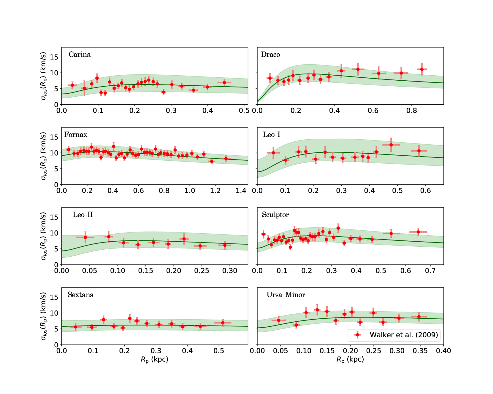
Figure 1: Radial profiles of the line-of-sight velocity dispersions of the eight dSphs listed in Table 1. The red circles with error bars show the measured $\sigma_{\mathrm{los,\,obs}}(r_{i})$ from Walker et al. (2009c). The green solid lines show the model profiles $\sigma_{\mathrm{los,\,th}}(\bm{\theta},r_{i})$ in $f(R)$ gravity adopting the best-fit parameters $\bm{\theta}=\{\delta,\xi,\beta,M_{*}/L\}$ listed in Table 2; the green shaded areas show the corresponding 1$\sigma$ spreads of the model profiles.

Galaxy	$D_{\odot}$	$D_{p}$	$\log(L_{\rm V})$	$r_{1/2}$	$M(<r_{\mathrm{last}})$	Ref.	$r_{\mathrm{tidal}}$	$\frac{r_{\mathrm{last}}}{r_{\mathrm{tidal}}}$	$\langle B-V\rangle$	$\langle V-I\rangle$	$M_{*}/L_{V}$
	(kpc)	(kpc)	($L_{\odot}$)	(pc)	($10^{7}M_{\odot}$)		(kpc)
(1)	(2)	(3)	(4)	(5)	(6)	(7)	(8)	(9)	(10)	(11)	(12)
Carina	105$\pm$6	$60^{+21}_{-16}$	5.57$\pm$0.20	273$\pm$45	$3.7^{+2.1}_{-1.8}$	[1, 2, 3, 15]	$\sim 2.0$	$\sim 2.0$	-	$1.1\pm 0.2$	$3.4\pm 2.9$
Draco	76$\pm$5	$28^{+12}_{-7}$	5.45$\pm$0.08	244$\pm$9	$26.4^{+18.6}_{-17.4}$	[3, 4, 5, 6, 15]	$\sim 1.7$	$\sim 1.0$	-	$1.4\pm 0.1$	$11.1\pm 4.7$
Fornax	147$\pm$12	$69^{+26}_{-18}$	7.31$\pm$0.12	792$\pm$58	$12.8^{+2.2}_{-5.6}$	[1, 2, 3, 15]	$\sim 2.8$	$\sim 1.7$	-	$1.3\pm 0.2$	$7.1\pm 6.0$
Leo I	$254^{+19}_{-16}$	$45^{+80}_{-34}$	6.74$\pm$0.12	298$\pm$29	$8.9^{+4.3}_{-5.2}$	[2, 3, 7, 8, 15]	$\sim 2.0$	$\sim 2.1$	-	$1.4\pm 0.1$	$8.8\pm 5.6$
Leo II	233$\pm$15	$45^{+121}_{-30}$	5.87$\pm$0.12	219$\pm$52	$1.7^{+1.9}_{-1.2}$	[2, 3, 9, 10, 15]	$\sim 1.1$	$\sim 2.6$	-	$0.6\pm 0.2$	$0.4\pm 0.4$
Sculptor	86$\pm$6	$50^{+15}_{-10}$	6.36$\pm$0.20	311$\pm$46	$10.0^{+3.2}_{-5.0}$	[2, 3, 11, 15]	$\sim 2.3$	$\sim 2.1$	-	$1.1\pm 0.1$	$3.6\pm 2.0$
Sextans	86$\pm$4	$71^{+11}_{-12}$	5.64$\pm$0.20	748$\pm$66	$2.0^{+1.0}_{-0.7}$	[2, 3, 12, 15]	$\sim 1.9$	$\sim 1.9$	-	$1.4\pm 0.1$	$8.5\pm 3.3$
Ursa Minor	76$\pm$4	$29^{+8}_{-6}$	5.45$\pm$0.20	398$\pm$44	$4.4^{+2.9}_{-2.0}$	[2, 3, 13, 14, 15]	$\sim 1.0$	$\sim 1.3$	$0.5\pm 0.3$	-	$1.2\pm 1.3$

Table 1: Observational properties of the eight dSphs analysed in this work. Columns (2) and (3): distance of the dSph from the observer and distance of the pericentre of the dSph orbit around the Milky Way from the Milky Way center of mass; Column (4): total $V$-band luminosity; Column (5): half-light radius; Column (6): total mass, estimated by Walker et al. (2009c) assuming Newtonian gravity, within the outermost data point of the velocity dispersion profile; Column (7): sources of the observational data: [1] Pietrzyński et al. (2009), [2] Irwin & Hatzidimitriou (1995), [3] Walker et al. (2009c), [4] Bonanos et al. (2004), [5] Martin et al. (2008), [6] Walker et al. (2007), [7] Bellazzini et al. (2004), [8] Mateo et al. (2008), [9] Bellazzini et al. (2005), [10] Koch et al. (2007), [11] Pietrzyński et al. (2008), [12] Lee et al. (2009), [13] Carrera et al. (2002), [14] Walker et al. (2009b), [15] Fritz et al. (2018); Columns (8), and (9): tidal radius in Newtonian gravity [Eq. (20)] adopting the total Milky Way mass $M=1.08_{-0.14}^{+0.20}\times 10^{12}M_{\odot}$ (Cautun et al., 2020) and radius of the last data point of the velocity dispersion profile; Column (10), and (11): average values of the $B-V$ and $V-I$ indexes (see Sect. 3.2); Column (12): stellar mass-to-light ratios in the $V$-band (see Sect. 3.2).

3.2 Expected mass-to-light ratios

In Newtonian gravity, the mass-to-light ratio of a dSph can be adjusted to any value depending on the mass associated to the dark matter halo embedding the stellar component. In our $f(R)$ model, where dark matter is absent, the mass-to-light ratio must be consistent with the value expected for the stellar population of the dSph. Nevertheless, in our MCMC analysis that we illustrate below, we still allow the mass-to-light ratio to vary as a free parameter within a limited range. Here, we derive the expected ratio around which we allow the mass-to-light ratio to vary in our MCMC analysis.

According to stellar population synthesis models (Bell & de Jong, 2001), Portinari et al. (2003, 2004) derived relations between the mass-to-light ratio and the colour of a stellar population. We consider the following relations (Appendix B in Portinari et al. 2004)

$$(B-V):\quad\log\biggl{(}\frac{M_{*}}{L_{X}}\biggr{)}=s_{X}[(B-V)-0.6]+q_{X}\,,$$ (21)

$$(V-I):\quad\log\biggl{(}\frac{M_{*}}{L_{X}}\biggr{)}=s_{X}[(V-I)-0.9]+q_{X}\,.$$ (22)

Here, the subscript $X$ indicates the magnitude band ($V$ in our case), and the coefficient $s_{X}$ is equal to 1.29 and 1.66 for the $(B-V)$ and $(V-I)$ relations, respectively. The parameter $q_{X}$ is estimated by assuming a Kennicutt Initial Mass Function (Kennicutt, 1983) in the range $[0.1-100]M_{\odot}$, and it is equal to 0.028 and -0.002 for the $(B-V)$ and $(V-I)$ relations, respectively.

We estimate the expected stellar mass-to-light ratio $M_{*}/L_{V}$ from the measured colour indexes of each dSph. These colour indexes are the average of the colour indexes measured in different regions of the same galaxy. We adopt the spread of these measures as their uncertainties. The colour indexes of Carina, Fornax, Sculptor, and Sextans are from the Magellan/MMFS Survey (Walker et al., 2009a), the colour indexes of Leo I, Leo II, Draco, and Ursa Major are from Mateo et al. (2008); Lépine et al. (2011); Kinemuchi et al. (2008); Olszewski & Aaronson (1985), respectively. For each galaxy, we estimate the stellar mass-to-light ratio $M_{*}/L_{V}$ and its error by randomly sampling $N=1000$ colour indexes from a Gaussian distribution whose mean and width are the average index and its corresponding uncertainty. Equations (21) or (22) thus provide $N$ values of $M_{*}/L_{V}$. Table 1 lists the average of these $M_{*}/L_{V}$ values and their spread.

3.3 Monte Carlo Markov Chains

Modeling the observed velocity dispersion profile $\sigma_{\mathrm{los,\,obs}}(r)$ measured by Walker et al. (2009d) with the profile $\sigma_{\mathrm{los,\,th}}(r)$ expected in $f(R)$ gravity requires the estimation of the set of four free parameters $\bm{\theta}=$ {$\delta$, $\xi$, $\beta$, $M_{*}/L_{V}$}. We explore this four-dimensional parameter space with the MCMC algorithm emcee (Foreman-Mackey et al., 2013).

We assign a uniform prior distribution to the first three parameters in the ranges $\delta\in(-1;10]$, $\xi\in[0.01,10^{3}]$ Mpc^-1, and $\beta\in[-100,1)$. For each dSph, for the mass-to-light ratio $M_{*}/L_{V}$, we set a Gaussian prior with mean and dispersion derived in Sect. 3.2 and listed in Column (13) of Table 1. We adopt the posterior probability distribution

$$-2\log P(\bm{\theta}|\textrm{ data})\propto \sum_{i}\biggl{[}\frac{\sigma_{\mathrm{los,\,th}}(\bm{\theta},\,r_{i})-\sigma_{\mathrm{los,\,obs}}(r_{i})}{\Delta\sigma_{\mathrm{los,\,obs}}(r_{i})}\biggr{]}^{2}\,,$$ (23)

where $\Delta\sigma_{\mathrm{los,\,obs}}(r_{i})$ are the observational uncertainties. We consider that our chains have converged when (1) all the chains are longer than 100 times the autocorrelation time, and (2) the autocorrelation time varies by less than 1% (for more details we refer to Sect. 3 in De Martino et al. 2022).

4 Results

In our MCMC analysis, we employ 12 chains with random starting points selected from the prior distributions described in Sect. 3.3. Figure 2 shows the post burn-in posterior distributions of the parameters for each dSph derived with all these 12 chains. We adopt the median of each posterior distribution as the best estimate of each of our free parameter, and the range within the 15.9 and 84.1 percentiles of each distribution as the 68% confidence interval. These values are listed in Table 2.

In Fig. 1, the green solid lines show the velocity dispersion profiles obtained with the parameters listed in Table 2. The green shaded areas show the 1$\sigma$ uncertainties of the profiles. These uncertainties are the spread of 1,000 profiles derived by randomly sampling 1,000 times the input parameters within their posterior distribution obtained from our MCMC analysis. The model appears to properly describe the observed profiles measured by Walker et al. (2009d) and shown by the red circles with error bars.

In the standard model, the observed velocity dispersion profiles are modeled by assuming the presence of dark matter. In $f(R)$ gravity, the role played by the dark matter is played by the two parameters $\xi$ and $\delta$ listed in Table 2. This table also lists the first two coefficients $f^{\prime}_{0}$ and $f^{\prime\prime}_{0}$ of the Taylor expansion of the function $f(R)$ (see Sect. 2.3). For all the dSphs, the parameter $\xi$ appearing in the exponential term of the gravitational potential [Eq. (14)] is $\xi\sim 1$ Mpc^-1, and this Yukawa term is thus negligible on the scale of a few kiloparsec, corresponding to the size of the dSphs. It follows that modelling the kinematics of the stars in $f(R)$ gravity requires large departures of $\delta$ from the value $\delta=0$ of standard gravity. Indeed, for all the dSphs, the best value is close to the lower limit $\delta=-1$, and the value $\delta=0$ is excluded at $\sim 30\sigma$ for Carina, Draco, Leo I, and Sextans, and at $\sim 250\sigma$ for Fornax and Ursa Minor.

The absence of dark matter requires the mass-to-light ratio $M_{*}/L_{V}$ to be within the values expected from stellar population synthesis models. Our Gaussian priors set around these values guarantee that this conditions is verified, as shown in Fig. 2. The velocity field of the stars inferred in $f(R)$ gravity is similar to the field inferred in standard gravity: the velocity anisotropy parameter $\beta$ we derive is within $2.5\sigma$ at most from the values $\beta_{\mathrm{NFW}}$ derived by Walker et al. (2009d) assuming a dark matter halo with a NFW density profile in standard gravity.

Figure 4 compares our estimates of $\delta$ and $\xi$ for the eight dSphs. For $\xi^{-1}$, the dSphs have fully consistent values with mean $\xi^{-1}=1.2^{+18.6}_{-0.9}$ Mpc, whereas $\delta$ clusters around two values $\overline{\delta}=-0.986\pm 0.002$ and $\overline{\delta}=-0.92\pm 0.01$; these two values disagree by $6\sigma$. This discrepancy is not consistent with the expectations of $f(R)$ gravity: although $\delta$ and $\xi$ are not universal parameters, they should assume roughly the same values within the same class of objects (Capozziello & de Laurentis, 2011; Capozziello & De Laurentis, 2012). This tension might be alleviated by improving the model of the dSphs: in our analysis we assume non-rotating spherically symmetric galaxies, a single stellar population, and velocity anisotropy parameter and mass-to-light ratio constant with radius. These assumptions clearly are simplistic: they might introduce systematic errors and be responsible for these two wildly different values of $\delta$.

In the literature, the gravitational potential we use here [Eq.(14)] was only adopted by Capozziello et al. (2009) to model the mass profile of a sample of 12 X-ray galaxy clusters. The estimates of $\delta$ and $\xi$ for the X-ray clusters are shown in Fig. 4. Both $\delta$ and $\xi$ appear to depend on the cluster, at odds with the $f(R)$ expectations of consistent values within the same class of objects. The uncertainties on the estimates of $\delta$ and $\xi$ of the clusters are substantially smaller than the uncertainties for the dSphs, where the variation of the parameter values from dSph to dSph appears to be limited. The large fluctuations for the clusters might suggest that, in the cluster analysis, either the random errors are underestimated or some systematic error is present, or both.

The presence of possible unidentified systematic errors is indeed suggested by the correlation, for the clusters, between the two parameters $\xi$ and $\delta$ shown in Fig. 5. The linear correlation coefficient is $\rho=0.90$ with a $p$-value, which is the probability of measuring $\rho$ from uncorrelated quantities, $p=7\times 10^{-5}$. This correlation indicates that the pair $(\delta,\xi)$ depends on the cluster. In principle, this correlation cannot be physically motivated in $f(R)$ gravity, unless we wish to introduce substantial complications in the theory. On the contrary, the values of the dSphs show no correlation ($\rho=0.14$ and $p=0.75$), supporting the conclusion that systematic errors are less relevant in our dSph analysis than in the cluster analysis.

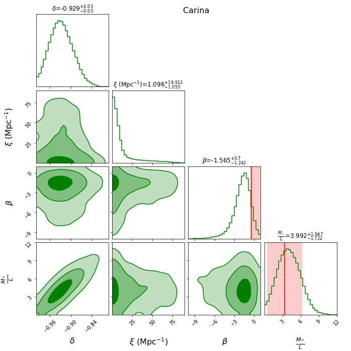
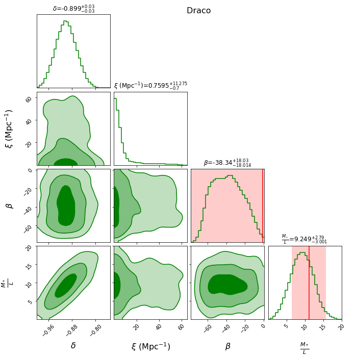
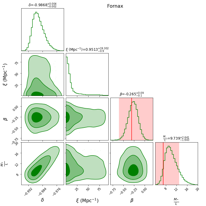
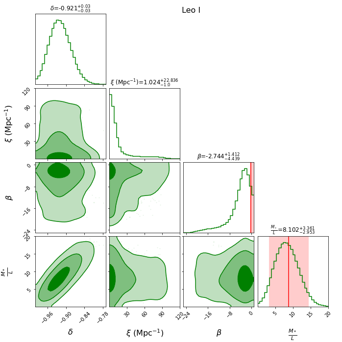
Figure 2: MCMC posterior distributions of the set of parameters $\bm{\theta}=\{\delta,\xi,\beta,M_{*}/L\}$ for each dSph. The shaded areas with decreasing darkness depict the 68%, 95%, and 99% confidence regions of the posterior distributions, respectively. The medians of the posterior distributions with their 68% confidence intervals are reported on top of each column. The red shaded areas in the panels corresponding to the velocity anisotropy parameter $\beta$ indicate the best fit values and the $1\sigma$ uncertainties of $\beta_{\mathrm{NFW}}$ as reported in Walker et al. (2009d) and listed in Column (7) of Table 1. The red shaded areas in the panels corresponding to the mass-to-light ratio $M_{*}/L_{V}$ indicate the values expected from the stellar population synthesis model listed in Column (13) of Table 1.

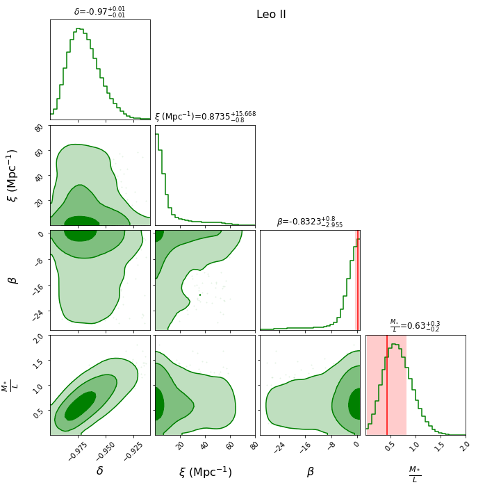
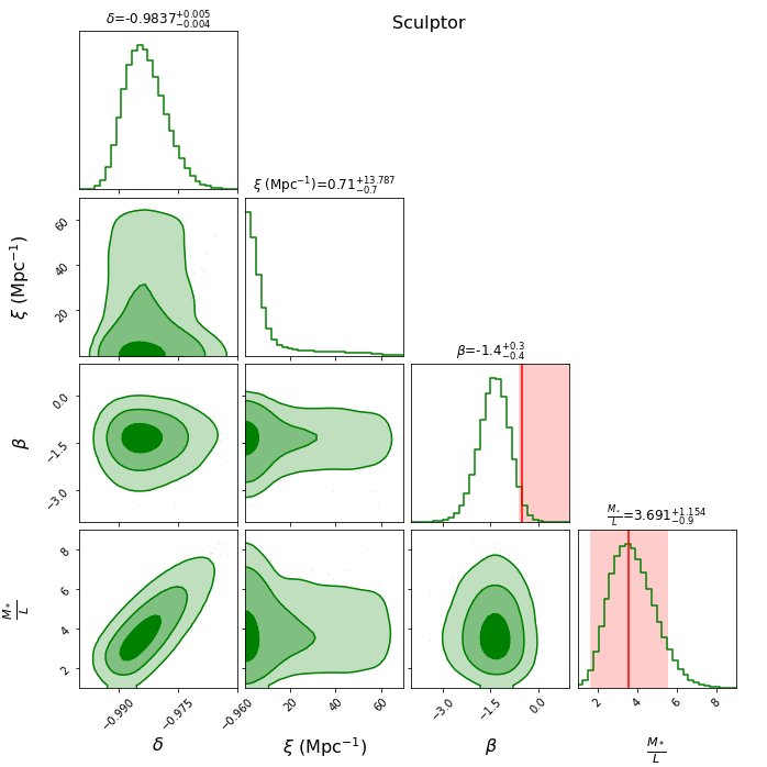
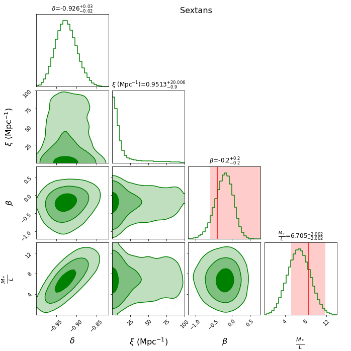
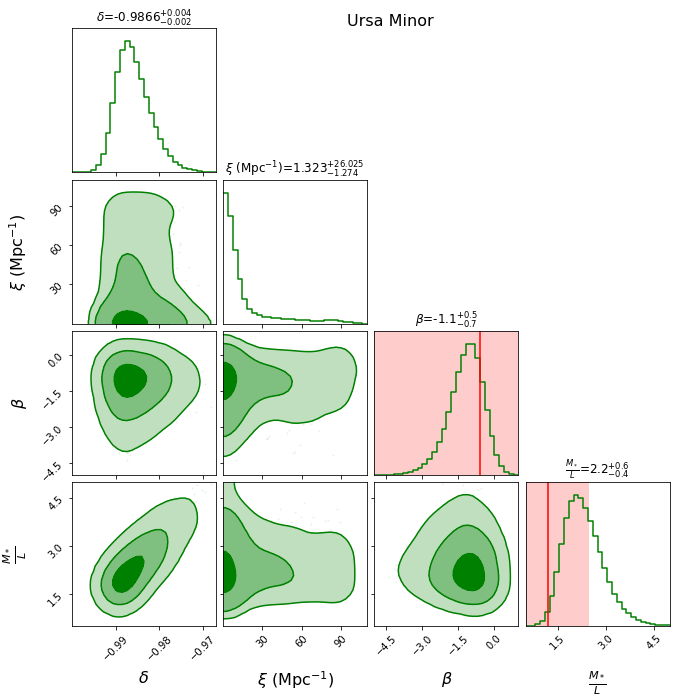
Figure 3: Continued.

Galaxy	$\delta$	$\xi$	$\beta$	$M_{*}/L_{V}$	$f^{\prime}_{0}$	$f^{\prime\prime}_{0}$	$\beta_{\mathrm{NFW}}$
		($\rm{Mpc}^{-1})$				($\rm{Mpc}^{2}$)
(1)	(2)	(3)	(4)	(5)	(6)	(7)	(8)
Carina	$-0.93\pm 0.03$	$1^{+20}_{-1}$	$-1.6^{+0.7}_{-1.3}$	$4.0^{+1.9}_{-1.7}$	$0.08^{+0.05}_{-0.03}$	$0.001^{+0.05}_{-2.77}$	$-0.4^{+0.6}_{-0.2}$
Draco	$-0.90\pm 0.03$	$0.8^{+11.3}_{-0.7}$	$-38\pm 18$	$9.3^{+2.8}_{-3.0}$	$0.10\pm 0.03$	$0.0006^{+3.615}_{-0.0006}$	$-0.6^{+0.8}$
Fornax	$-0.987^{+0.004}_{-0.002}$	$1^{+19}_{-1}$	$-0.27^{+0.09}_{-0.1}$	$9.7^{+2.6}_{-1.6}$	$0.014^{+0.005}_{-0.002}$	$0.001^{+0.90}_{-0.001}$	$-0.3^{+0.3}_{-0.3}$
Leo I	$-0.92\pm 0.03$	$1^{+23}_{-1}$	$-2.7^{+1.4}_{-4.4}$	$8.1^{+3.6}_{-3.0}$	$0.08\pm 0.03$	$0.01^{+6.57}_{-0.01}$	$-0.2^{+0.6}_{-0.3}$
Leo II	$-0.97\pm 0.01$	$0.8^{+15.7}_{-0.8}$	$-0.8^{+0.8}_{-3.0}$	$0.6^{+0.3}_{-0.2}$	$0.03^{+0.02}_{-0.01}$	$0.002^{+1.68}_{-0.002}$	$+0.3_{-0.9}$
Sculptor	$-0.985^{+0.005}_{-0.004}$	$0.7^{+13.8}_{-0.7}$	$-1.4^{+0.3}_{-0.4}$	$3.7^{+1.2}_{-0.9}$	$0.016^{+0.005}_{-0.004}$	$0.00007^{+0.005}_{-0.00007}$	$-0.5^{+0.5}_{-0.1}$
Sextans	$-0.93^{+0.03}_{-0.02}$	$1^{+20}_{-1}$	$-0.2\pm 0.2$	$6.7\pm 2.0$	$0.07^{+0.03}_{-0.02}$	$0.01^{+6.61}_{-0.01}$	$-0.4^{+0.6}_{-0.2}$
Ursa Minor	$-0.978^{+0.004}_{-0.003}$	$1^{+26}_{-1}$	$-1.1^{+0.5}_{-0.7}$	$2.2^{+0.6}_{-0.4}$	$0.013^{+0.004}_{-0.002}$	$0.001^{+1.0}_{-0.001}$	$-0.6^{+0.8}$

Table 2: MCMC estimates of the set of parameters $\bm{\theta}=\{\delta,\xi,\beta,M_{*}/L_{V}\}$. Column (1): dSph name; Columns (2)-(5): median and 1$\sigma$ confidence interval; Columns (6) and (7): Taylor coefficients $f^{\prime}_{0}$ and $f^{\prime\prime}_{0}$, with 1$\sigma$ confidence intervals; Columns (8): velocity anisotropy parameter $\beta_{\mathrm{NFW}}$ under the assumption of a Navarro-Frank-White model for the dark matter halo in standard gravity (Walker et al., 2009d).

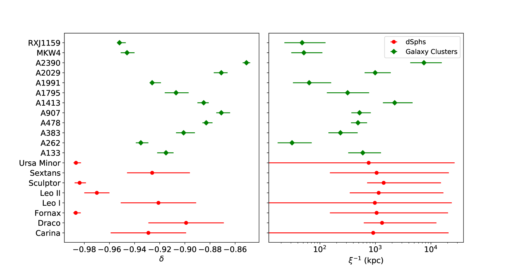
Figure 4: MCMC estimates of the parameters $\delta$ (left panel) and $\xi$ (right panel) and their 1$\sigma$ confidence intervals for the dSphs analysed in this paper (red circles with error bars) and for the galaxy clusters analysed by Capozziello et al. (2009) (green circles with error bars).

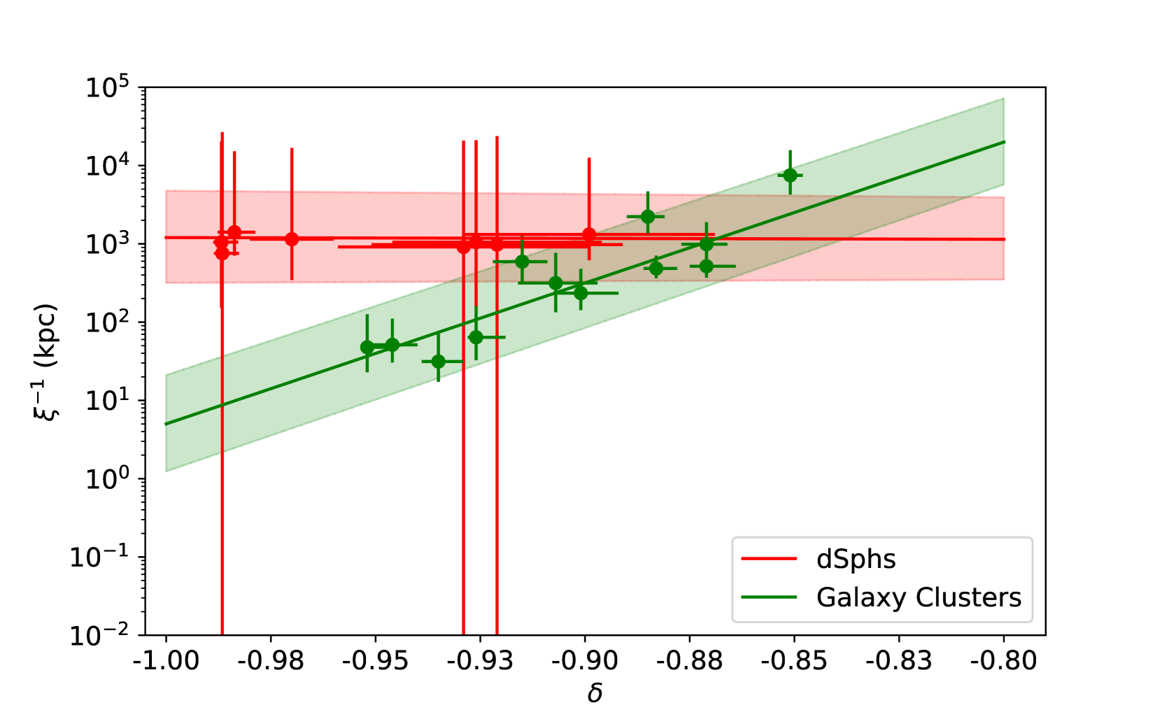
Figure 5: Correlation between the two parameters $\xi^{-1}$ and $\delta$ for dSphs (red solid line) and galaxy clusters (green solid line), respectively. The solid lines and shaded areas are the least squares fits and their 1-$\sigma$ spreads.

5 Discussion and Conclusions

Modifications of GR have been extensively studied to overcome some of the tensions affecting the $\Lambda$CDM model (De Martino et al., 2020; Peebles, 2022). $f(R)$ gravity is one of the most tested theories of gravity on extra-galactic and cosmological scales. Indeed, the extra degrees of freedom that arise in $f(R)$ can easily explain the accelerated expansion of the Universe (Starobinsky, 2007; Hu & Sawicki, 2007; Amendola & Tsujikawa, 2008; Miranda et al., 2009; De Martino et al., 2015; Lazkoz et al., 2018; Calzà et al., 2018), whereas $f(R)$ reduces to GR on the Solar System scale (De Felice & Tsujikawa, 2010). On the intermediate scale of galaxies, the ability of $f(R)$ gravity to describe the dynamics of cosmic structure without the aid of dark matter, as in the standard model, is substantially less investigated.

In the weak-field limit, $f(R)$ introduces a modification to the Newtonian gravitational potential that is parameterized by the two parameters $\delta$ and $\xi$ (Capozziello et al., 2009; Banerjee et al., 2017). Here, we contributed to the quest of the ability of these two parameters to play the role of dark matter by assessing whether $f(R)$ gravity can describe the dynamics of eight dSphs. We modelled the observed velocity dispersion profiles of the dSph stars with the Jeans equation (Sect.  3.3). Our results are based on a set of simplifying assumptions: a non-rotating spherically symmetric galaxy, a single stellar population, a mass-to-light ratio and a velocity anisotropy parameter $\beta$ constant with radius.

Our analysis returns a length scale of the Yukawa potential, $\xi^{-1}=1.2^{+18.6}_{-0.9}$ Mpc for all the galaxies. This result is reassuring for two reasons: (1) a single value of $\xi^{-1}$ is valid for the entire dSph sample, as expected in $f(R)$ gravity within the same class of objects; (2) the value of $\xi^{-1}$ guarantees that the extra-degrees of freedom do not play any relevant role in the dynamics of self-gravitating systems on scale below $\sim 1$ Mpc, where the effects of the accelerated expansion of the Universe or the effects of a fifth force are lacking. Our result confirms previous analyses. For instance, De Martino (2016) found $\xi^{-1}\sim 1$ Mpc by fitting the SZ temperature anisotropy profile of the Coma cluster. Capozziello et al. (2009) and Napolitano et al. (2012) also found similar values of $\xi^{-1}$ by modelling the mass profile of 12 X-ray galaxy clusters and the stellar kinematics of elliptical galaxies, respectively. Actually, the estimated values of $\xi^{-1}$ in Capozziello et al. (2009) range from 100 kpc to 10 Mpc depending on the systems. However, these fluctuations of $\xi^{-1}$ may be due to a simplistic modeling based on the assumption of a phenomenological X-ray gas density whose parameters are not fitted together with the $f(R)$-gravity parameters.

On the other hand, our result on $\delta$ suggests a possible tension for $f(R)$ gravity. The parameter $\delta$ controls the intensity of the gravitational field. In Eq. (14) for the modified gravitational potential of an extended mass distribution, the term $(1+\delta)^{-1}$ multiplies the mass density: $\delta$ can thus mimic an increasing dark matter content by assuming values increasingly close to $-1$.

The values of $\delta$ we find for the dSph sample have a bimodal distribution peaking around two values $\overline{\delta}=-0.986\pm 0.002$ and $\overline{\delta}=-0.92\pm 0.01$. These values differ by 6-$\sigma$. Therefore, unlike $\xi$, $\delta$ does not assume a single value which is valid for all the dSphs in the sample. Our analysis rather suggests that different values of $\delta$ are required for different objects within the same class, at odds with the expectations from $f(R)$ gravity.

Different values of $\delta$ are expected in different classes of objects but not within the same class of objects. For example, for gravitational systems where dark matter is not required in standard gravity, like stellar systems, $\delta$ is expected to be sufficiently close to zero to guarantee negligible departures, if any, from the standard Newtonian dynamics. Indeed, De Martino et al. (2021) showed that reproducing the orbital motion of the S2 star around the supermassive black hole in the centre of the Galaxy requires $\delta=-0.01_{-0.14}^{+0.61}$, which is compatible with zero at 1-$\sigma$. On the contrary, for systems dominated by dark matter in the standard model, like clusters of galaxies, $\delta$ is close to $-1$. For example, Capozziello et al. (2009) found $\delta$ in the range $[-0.95,-0.85]$ for the X-ray clusters mentioned above. The disagreement we find for the two values of $\delta$ for the dSphs suggests a severe tension for $f(R)$ gravity.

In principle, more sophisticated extended theories of gravity might properly describe the kinematics of dwarf galaxies and reduce, or completely eliminate, the tension we find here. For example, a scalar-tensor $f(R,\phi)$ theory, a fourth-order theory of gravity non-minimally coupled with a massive scalar field $\phi$, generates Yukawa-like corrections to the Newtonian gravitational potential in the weak-filed limit similarly to $f(R)$ gravity. The correction terms are related to the extra degrees of freedom and generate gravitational forces that mimic the gravitational field of the dark matter halo and accommodate the rotation curves of spiral galaxies (Stabile & Capozziello, 2013). It is likely, but still to be proved, that similar correction terms can also describe the dynamics of dwarf galaxies.

Alternatively, improved models of the dwarf galaxies, where our simplifying assumptions are dropped, may be sufficient to remove the tension for $f(R)$ gravity. Further insights will come from observations: a future Theia-like astrometric mission (Malbet et al., 2016; The Theia Collaboration et al., 2017; Malbet et al., 2019, 2021) will provide high precision measures of the proper motion of the dSph stars. Similarly to what we expect for the core-cusp problem (De Martino et al., 2022), these additional information will decrease the current uncertainties on the estimate of $\xi^{-1}$, and either confirm or remove the tension on $\delta$ we find here.

Data Availability Statement

Data are publicly available in (Walker et al., 2007; Walker et al., 2009a; Walker et al., 2009b, c; Walker et al., 2009d).

References

- Amendola & Tsujikawa (2008) Amendola L., Tsujikawa S., 2008, Physics Letters B, 660, 125
- Banerjee et al. (2017) Banerjee S., Shankar S., Singh T. P., 2017, J. Cosmology Astropart. Phys., 2017, 004
- Bell & de Jong (2001) Bell E. F., de Jong R. S., 2001, ApJ, 550, 212
- Bellazzini et al. (2004) Bellazzini M., Gennari N., Ferraro F. R., Sollima A., 2004, MNRAS, 354, 708
- Bellazzini et al. (2005) Bellazzini M., Gennari N., Ferraro F. R., 2005, MNRAS, 360, 185
- Binney & Tremaine (2008) Binney J., Tremaine S., 2008, Galactic Dynamics: Second Edition
- Bonanos et al. (2004) Bonanos A. Z., Stanek K. Z., Szentgyorgyi A. H., Sasselov D. D., Bakos G. Á., 2004, AJ, 127, 861
- Boylan-Kolchin et al. (2011) Boylan-Kolchin M., Bullock J. S., Kaplinghat M., 2011, MNRAS, 415, L40
- Bullock & Boylan-Kolchin (2017) Bullock J. S., Boylan-Kolchin M., 2017, ARA&A, 55, 343
- Calzà et al. (2018) Calzà M., Rinaldi M., Sebastiani L., 2018, European Physical Journal C, 78, 178
- Capolupo (2017) Capolupo A., 2017, Galaxies, 5, 98
- Capozziello & De Laurentis (2012) Capozziello S., De Laurentis M., 2012, Annalen der Physik, 524, 545
- Capozziello & Tsujikawa (2008) Capozziello S., Tsujikawa S., 2008, Phys. Rev. D, 77, 107501
- Capozziello & de Laurentis (2011) Capozziello S., de Laurentis M., 2011, Phys. Rep., 509, 167
- Capozziello et al. (2007) Capozziello S., Stabile A., Troisi A., 2007, Phys. Rev. D, 76, 104019
- Capozziello et al. (2009) Capozziello S., de Filippis E., Salzano V., 2009, MNRAS, 394, 947
- Carrera et al. (2002) Carrera R., Aparicio A., Martínez-Delgado D., Alonso-García J., 2002, AJ, 123, 3199
- Cautun et al. (2020) Cautun M., et al., 2020, MNRAS, 494, 4291
- Cognola et al. (2008) Cognola G., Elizalde E., Nojiri S., Odintsov S. D., Sebastiani L., Zerbini S., 2008, Phys. Rev. D, 77, 046009
- De Felice & Tsujikawa (2010) De Felice A., Tsujikawa S., 2010, Living Reviews in Relativity, 13, 3
- De Laurentis & De Martino (2013) De Laurentis M., De Martino I., 2013, MNRAS, 431, 741
- De Laurentis et al. (2018) De Laurentis M., De Martino I., Lazkoz R., 2018, Phys. Rev. D, 97, 104068
- De Martino (2016) De Martino I., 2016, Phys. Rev. D, 93, 124043
- De Martino et al. (2014) De Martino I., De Laurentis M., Atrio-Barandela F., Capozziello S., 2014, MNRAS, 442, 921
- De Martino et al. (2015) De Martino I., De Laurentis M., Capozziello S., 2015, Universe, 1, 123
- De Martino et al. (2018) De Martino I., Lazkoz R., De Laurentis M., 2018, Phys. Rev. D, 97, 104067
- De Martino et al. (2020) De Martino I., Chakrabarty S. S., Cesare V., Gallo A., Ostorero L., Diaferio A., 2020, Universe, 6, 107
- De Martino et al. (2021) De Martino I., della Monica R., De Laurentis M., 2021, Phys. Rev. D, 104, L101502
- De Martino et al. (2022) De Martino I., Diaferio A., Ostorero L., 2022, Monthly Notices of the Royal Astronomical Society
- Del Popolo & Le Delliou (2017) Del Popolo A., Le Delliou M., 2017, Galaxies, 5, 17
- Di Valentino et al. (2021) Di Valentino E., et al., 2021, Classical and Quantum Gravity, 38, 153001
- Foreman-Mackey et al. (2013) Foreman-Mackey D., Hogg D. W., Lang D., Goodman J., 2013, Publications of the Astronomical Society of the Pacific, 125, 306
- Fritz et al. (2018) Fritz T. K., Battaglia G., Pawlowski M. S., Kallivayalil N., van der Marel R., Sohn S. T., Brook C., Besla G., 2018, A&A, 619, A103
- Hu & Sawicki (2007) Hu W., Sawicki I., 2007, Phys. Rev. D, 76, 064004
- Irwin & Hatzidimitriou (1995) Irwin M., Hatzidimitriou D., 1995, MNRAS, 277, 1354
- Kennicutt (1983) Kennicutt R. C. J., 1983, ApJ, 272, 54
- Khoury & Weltman (2004) Khoury J., Weltman A., 2004, Phys. Rev. D, 69, 044026
- Kinemuchi et al. (2008) Kinemuchi K., Harris H. C., Smith H. A., Silbermann N. A., Snyder L. A., La Cluyzé A. P., Clark C. L., 2008, AJ, 136, 1921
- King (1962) King I., 1962, AJ, 67, 471
- Koch et al. (2007) Koch A., Kleyna J. T., Wilkinson M. I., Grebel E. K., Gilmore G. F., Evans N. W., Wyse R. F. G., Harbeck D. R., 2007, AJ, 134, 566
- Lazkoz et al. (2018) Lazkoz R., Ortiz-Baños M., Salzano V., 2018, The European Physical Journal C, 78
- Lee et al. (2009) Lee M. G., Yuk I.-S., Park H. S., Harris J., Zaritsky D., 2009, ApJ, 703, 692
- Lépine et al. (2011) Lépine S., Koch A., Rich R. M., Kuijken K., 2011, ApJ, 741, 100
- Li & Barrow (2007) Li B., Barrow J., 2007, Phys. Rev. D, 75, 084010
- Łokas & Mamon (2003) Łokas E. L., Mamon G. A., 2003, MNRAS, 343, 401
- Malbet et al. (2016) Malbet F., et al., 2016, in MacEwen H. A., Fazio G. G., Lystrup M., Batalha N., Siegler N., Tong E. C., eds, Society of Photo-Optical Instrumentation Engineers (SPIE) Conference Series Vol. 9904, Space Telescopes and Instrumentation 2016: Optical, Infrared, and Millimeter Wave. p. 99042F, doi:10.1117/12.2234425
- Malbet et al. (2019) Malbet F., et al., 2019, arXiv e-prints, p. arXiv:1910.08028
- Malbet et al. (2021) Malbet F., et al., 2021, Experimental Astronomy, 51, 845
- Mamon & Boué (2010) Mamon G. A., Boué G., 2010, MNRAS, 401, 2433
- Mamon & Łokas (2005) Mamon G. A., Łokas E. L., 2005, MNRAS, 363, 705
- Martin et al. (2008) Martin N. F., de Jong J. T. A., Rix H.-W., 2008, ApJ, 684, 1075
- Mateo (1998) Mateo M. L., 1998, ARA&A, 36, 435
- Mateo et al. (2008) Mateo M., Olszewski E. W., Walker M. G., 2008, ApJ, 675, 201
- Miranda et al. (2009) Miranda V., Jorás S. E., Waga I., Quartin M., 2009, Physical Review Letters, 102, 221101
- Muñoz et al. (2008) Muñoz R. R., Majewski S. R., Johnston K. V., 2008, ApJ, 679, 346
- Napolitano et al. (2012) Napolitano N. R., Capozziello S., Romanowsky A. J., Capaccioli M., Tortora C., 2012, ApJ, 748, 87
- Navarro et al. (1996) Navarro J. F., Frenk C. S., White S. D. M., 1996, ApJ, 462, 563
- Nojiri & Odintsov (2007) Nojiri S., Odintsov S. D., 2007, Physics Letters B, 657, 238
- Nojiri & Odintsov (2011) Nojiri S., Odintsov S. D., 2011, Phys. Rep., 505, 59
- Nojiri et al. (2017) Nojiri S., Odintsov S. D., Oikonomou V. K., 2017, Phys. Rep., 692, 1
- Olszewski & Aaronson (1985) Olszewski E. W., Aaronson M., 1985, AJ, 90, 2221
- Peebles (2022) Peebles P. J. E., 2022, arXiv e-prints, p. arXiv:2208.05018
- Piatek et al. (2007) Piatek S., Pryor C., Bristow P., Olszewski E. W., Harris H. C., Mateo M., Minniti D., Tinney C. G., 2007, AJ, 133, 818
- Pietrzyński et al. (2008) Pietrzyński G., et al., 2008, AJ, 135, 1993
- Pietrzyński et al. (2009) Pietrzyński G., Górski M., Gieren W., Ivanov V. D., Bresolin F., Kudritzki R.-P., 2009, AJ, 138, 459
- Planck Collaboration et al. (2014) Planck Collaboration et al., 2014, A&A, 571, A1
- Planck Collaboration et al. (2020a) Planck Collaboration et al., 2020a, A&A, 641, A5
- Planck Collaboration et al. (2020b) Planck Collaboration et al., 2020b, A&A, 641, A6
- Planck Collaboration et al. (2020c) Planck Collaboration et al., 2020c, A&A, 641, A7
- Portinari et al. (2003) Portinari L., Sommer-Larsen J., Tantalo R., 2003, Ap&SS, 284, 723
- Portinari et al. (2004) Portinari L., Sommer-Larsen J., Tantalo R., 2004, MNRAS, 347, 691
- Salucci et al. (2021) Salucci P., et al., 2021, Frontiers in Physics, 8, 579
- Sohn et al. (2007) Sohn S. T., et al., 2007, ApJ, 663, 960
- Stabile & Capozziello (2013) Stabile A., Capozziello S., 2013, Phys. Rev. D, 87, 064002
- Starobinsky (1980) Starobinsky A., 1980, Phys. Lett. B, 91, 99
- Starobinsky (2007) Starobinsky A., 2007, JETP Lett., 86, 157
- The Theia Collaboration et al. (2017) The Theia Collaboration et al., 2017, arXiv e-prints, p. arXiv:1707.01348
- Walker et al. (2007) Walker M. G., Mateo M., Olszewski E. W., Gnedin O. Y., Wang X., Sen B., Woodroofe M., 2007, ApJ, 667, L53
- Walker et al. (2009a) Walker M. G., Mateo M., Olszewski E. W., 2009a, AJ, 137, 3100
- Walker et al. (2009b) Walker M. G., Mateo M., Olszewski E. W., Sen B., Woodroofe M., 2009b, AJ, 137, 3109
- Walker et al. (2009c) Walker M. G., Belokurov V., Evans N. W., Irwin M. J., Mateo M., Olszewski E. W., Gilmore G., 2009c, ApJ, 694, L144
- Walker et al. (2009d) Walker M. G., Mateo M., Olszewski E. W., Peñarrubia J., Evans N. W., Gilmore G., 2009d, ApJ, 704, 1274
- Weinberg (1987) Weinberg S., 1987, Phys. Rev. Lett., 59, 2607
- Weinberg (1989) Weinberg S., 1989, Reviews of Modern Physics, 61, 1
- von Hoerner (1957) von Hoerner S., 1957, ApJ, 125, 451