Unsupervised Sentence Textual Similarity
with Compositional Phrase Semantics

Abstract

Measuring Sentence Textual Similarity (STS) is a classic task that can be applied to many downstream NLP applications such as text generation and retrieval. In this paper, we focus on unsupervised STS that works on various domains but only requires minimal data and computational resources. Theoretically, we propose a light-weighted Expectation-Correction (EC) formulation for STS computation. EC formulation unifies unsupervised STS approaches including the cosine similarity of Additively Composed (AC) sentence embeddings Arora et al. (2017), Optimal Transport (OT) Kusner et al. (2015), and Tree Kernels (TK) Le et al. (2018). Moreover, we propose the Recursive Optimal Transport Similarity (ROTS) algorithm to capture the compositional phrase semantics by composing multiple recursive EC formulations. ROTS finishes in linear time and is faster than its predecessors. ROTS is empirically more effective and scalable than previous approaches. Extensive experiments on 29 STS tasks under various settings show the clear advantage of ROTS over existing approaches. Detailed ablation studies demonstrate the effectiveness of our approaches.

1 Introduction

Sentence Textual Similarity (STS) measures the semantic equivalence between a pair of sentences, which is supposed to be consistent with human evaluation Agirre et al. (2012). STS is also an effective sentence-level semantic measure for many downstream tasks such as text generation and retrieval Wieting et al. (2019); Zhao et al. (2019); Nikolentzos et al. (2020); Çelikyilmaz et al. (2020). In this paper, we focus on unsupervised STS which is expected to compare texts of various domains but only requires minimal data and computational resources.

There are several typical ways to compute unsupervised STS, including 1) treat each sentence as an embedding by the Additive Composition (AC) Arora et al. (2017) of word vectors, then estimate the STS of two sentences by their cosine similarity; 2) treat each sentence as a probabilistic distribution of word vectors, then measure the distance between distributions. Notably, Optimal Transport (OT) Peyré and Cuturi (2019) is adopted to compute the STS Kusner et al. (2015). OT-based approaches search for the best alignment with respect to the word-level semantics and result in state-of-the-art solution Yokoi et al. (2020).

In this paper, we argue that phrase-level semantics should also be exploited to fully understand the sentences. For example, “optimal transport” should be considered as a mathematical term rather than two independent words. Specifically, the phrase chunk is composed of lower-level chunks and is usually represented as a node in tree structures. The aforementioned AC and OT-based STS methods are too shallow to include such structures. Tree Kernels (TK) Le et al. (2018) consider the parsed syntax labels. However, it boils down to syntax-based but sub-optimal word alignment under our comparison experiment.

Recent advancement of Pretrained Language Models (PLMs) also demonstrate the importance of contextualization Peters et al. (2018); Devlin et al. (2019); Ethayarajh (2019). PLMs can be further adopted to STS tasks by supervised fine-tuning Devlin et al. (2019), under carefully designed transfer learning Reimers and Gurevych (2019) or domain-adaptation Li et al. (2020); Gao et al. (2021). Without those treatments, the performances of PLM-based STSs are observed to be very poor Yokoi et al. (2020). Meanwhile, PLM-based STSs suffer from high computational costs to fit large amounts of high-quality data, which might prevent them from broader downstream scenarios.

In this paper, we propose a set of concepts and similarities to exploit the phrase semantics in the unsupervised setup. Our contributions are four folds:

Unified formulation

We unify three types of unsupervised STS models (AC Arora et al. (2017), OT Yokoi et al. (2020) and TK Le et al. (2018)) by the EC similarity in Section 3. EC similarity uncovers the strengths and weaknesses of the three approaches.

Phrase vectors and their alignment

We generalize the idea of word alignment to phrase alignment in Section 4. After the formal definition of Recursive Phrase Partition (RPP), we compose the phrase weights and vectors by those from finer-grained partitions under the invariant additive phrase composition and generalize the word alignment to phrase alignment. Empirical observations show that EC similarity is an effective formulation to interpolate the existing unsupervised STS, and yields better performances.

Recursive Optimal Transport

We propose the Recursive Optimal Transport Similarity (ROTS) in Section 5 based on the phrase alignment introduced in Section 4. ROTS computes the EC similarity at each phrase partition level and ensembles them. Notably, Prior Optimal Transport (Prior OT) is adopted to guide the finer-grained phrase alignment by the coarser-grained phrase alignment at each expectation step of EC similarity.

Extensive experiments

We show the comprehensive performance of ROTS on a wide spectrum of experimental settings in Section 6 and the Appendix, including 29 STS tasks, five types of word vectors, and three typical preprocessing setups. Specifically, ROTS is shown to be better than all other unsupervised approaches including $\mathrm{BERT}$ based STS in terms of both effectiveness and efficiency. Detailed ablation studies also show that our constructive definitions are sufficiently important and the hyper-parameters can be easily chosen to obtain the new SOTA performances.

2 Related Work

Embedding the symbolic words into continuous space to present their semantics Mikolov et al. (2013); Pennington et al. (2014); Bojanowski et al. (2017) is one of the breakthroughs of modern NLP. Notably, it shows that the vector (or semantics) of a phrase can be approximated by the additive composition of the vectors of its containing words Mikolov et al. (2013). Thus, word embeddings can be further utilized to describe the semantics of texts beyond the word level. Several strategies were proposed to provide sentence embeddings.

Additive Composition. Additive composition of word vectors Arora et al. (2017) forms effective sentence embeddings. The cosine similarity between the sentence embeddings has been shown to be a stronger STS under transferredWieting et al. (2016); Wieting and Gimpel (2018) and unsupervised settings Arora et al. (2017); Ethayarajh (2018) than most of the deep learning approaches Socher et al. (2013); Le and Mikolov (2014); Kiros et al. (2015); Tai et al. (2015).

Optimal Transport. By considering sentences as distributions of embeddings, the similarity between sentence pairs is the consequence of optimal transport of sentence distributions Kusner et al. (2015); Huang et al. (2016); Wu et al. (2018); Yokoi et al. (2020). OT models find the optimal alignment with respect to word semantics via their embeddings and have the SOTA performances Yokoi et al. (2020).

Syntax Information. One possible way to integrate contextual information in a sentence is to explicitly employ syntactic information. Recurrent neural networks Socher et al. (2013) were proposed to exploit the tree structures in the supervised setting but were sub-optimal than AC-based STS. Meanwhile, tree kernels Moschitti (2006); Croce et al. (2011) can measure the similarity between parsing trees. Most recently, ACV-tree kernels Le et al. (2018) combine word embedding similarities with parsed constituency labels. However, tree kernels compare all the sub-trees and suffer from high computational complexity.

Pretrained Language Models This paradigm produces contextualized sentence embeddings by aggregating the word embeddings repeatedly with the deep neural networks Vaswani et al. (2017) trained on large corpuses Devlin et al. (2019). In the unsupervised setting, PLMs are sub-optimal compared to SOTA OT-based models Yokoi et al. (2020). One of the common strategies to improve the performance is to adjust PLM-generated embedding according to a large amount of external data such as transfer learning Reimers and Gurevych (2019), flow Li et al. (2020), whitening Su et al. (2021), and contrastive learning Gao et al. (2021). However, this domain adaptation paradigm requires a complex training process and the performance is highly affected by the similarity between the target test data and external data Li et al. (2020); Gao et al. (2021).

3 Unification of Unsupervised STS Methods

Given a pair of sentences $(s^{(1)},s^{(2)})$, we are expected to estimate their similarity score $s\in[0,1]$. For sentence $s^{(1)}$ (or $s^{(2)}$), we have vector $\{v^{(1)}_{i}\}_{i=1}^{m}$ (or $\{v^{(2)}_{j}\}_{j=1}^{n}$) and weight $\{w^{(1)}_{i}\}_{i=1}^{m}$ (or $\{w^{(2)}_{j}\}_{j=1}^{n}$). We quickly review three types of unsupervised STS in Section 3.1 (see Figure 1 (a-c)), then unify them by the Expectation-Correction similarity in Section 3.2.

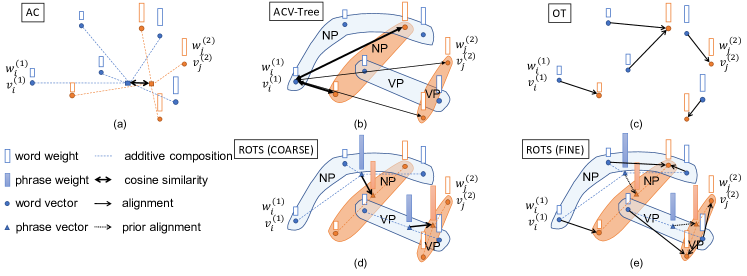
Figure 1: Different unsupervised STS methods with blue elements for $s^{(1)}$ and orange elements for $s^{(2)}$. (a) AC Arora et al. (2017): cosine similarity between additively composed sentence embeddings. (b) ACV-Tree Le et al. (2018): weighted averaging pairwise word similarity. Similarities from $v^{(1)}_{i}$ to vectors in $s^{(2)}$ are shown. More weights are assigned to pairs contained in the same constituency structure, indicated by thicker arrows. (c) OT Yokoi et al. (2020): compute the optimal transport alignment of words by solving problem (1). (d) ROTS at coarser hierarchy: the OT alignment of phrases vectors and weights. (e) ROTS at finer hierarchy: fine-level OT alignment based on the prior of coarse-level alignment in (d).

3.1 Review of Three Types of STS

Additive Composition (AC) AC methods Arora et al. (2017); Ethayarajh (2018) firstly compute the sentence embedding $x^{(\cdot)}=\sum_{i}w^{(\cdot)}_{i}v^{(\cdot)}_{i}$, then estimate the similarity by the cosine similarity $s_{AC}=\cos(x^{(1)},x^{(2)})$, see Figure 1 (a).

Optimal Transport (OT) Given pairwise word distance matrix $D=D_{ij}$ and two marginal distributions $\mu_{i}$ and $\nu_{i}$, the optimal transport alignment $\Gamma_{OT}$ is computed by solving the following minimization problem Kusner et al. (2015).

$$\Gamma_{OT}=\operatorname*{arg\,min}_{\Gamma_{ij}\geq 0}\sum_{ij}\Gamma_{ij}D_{ij},$$ (1)

$$\text{s.t. }\sum_{j}\Gamma_{ij}=\mu_{i},\sum_{i}\Gamma_{ij}=\nu_{j}.$$ (2)

The higher $\Gamma_{OT,ij}$ means that the alignment from $i$-th word in $s^{(1)}$ to $j$-th word in $s^{(2)}$ is preferred, because those two words are semantically closer, see Figure 1 (c). Different choices of $D,\mu,\nu$ lead to different distances. The SOTA OT-based STS is the Word Rotator’s Distance (WRD) Yokoi et al. (2020), which solves Problem (1) with $D_{ij}=1-\cos(w^{(1)}_{i},w^{(2)}_{j})$ and

$$\mu_{i}=\frac{w^{(1)}_{i}\|v^{(1)}_{i}\|_{2}}{\sum_{k}w^{(1)}_{k}\|v^{(1)}_{k}\|_{2}},$$ (3)

$$\nu_{j}=\frac{w^{(2)}_{j}\|v^{(2)}_{j}\|_{2}}{\sum_{k}w^{(2)}_{k}\|v^{(2)}_{k}\|_{2}}.$$

The similarity is

$$s_{OT}=\sum_{ij}\Gamma_{OT,ij}\cos(w^{(1)}_{i},w^{(2)}_{j}).$$ (4)

WRD is equivalent to AC if and only if each sentence contains one word Yokoi et al. (2020).

Tree Kernel (TK) General tree kernels compare the syntactic parsing information Moschitti (2006); Croce et al. (2011). Recently, ACV-Tree Le et al. (2018) combines word-level semantics with syntax information by a simplified partial tree kernel Moschitti (2006), see Figure 1 (b). Word similarities from the same structure, i.e. NP, are repeatedly counted and thus more important. Then the similarity score can be re-written as

$$s_{TK}=\sum_{ij}\Gamma_{TK,ij}\cos(w^{(1)}_{i},w^{(2)}_{j})$$ (5)

where $\Gamma_{TK}$ is the normalized weight matrix generated by the tree kernel .

3.2 Expectation Correction (EC)

Three approaches discussed above, though motivated in different ways, can be seen as a linear aggregation of pair-wise cosine similarities of words. We unified them into the following EC similarity with two steps called expectation and correction.

Table 1: The comparison of different approaches.

Method	Inter-sentence Expectation			Intra-sentence Correction	Tiime Complexity
	Word Semantics	Phrase Semantics	Syntax
AC Arora et al. (2017); Ethayarajh (2018)	✗	✗	✗	✓	$O(m+n)$
OT Kusner et al. (2015); Yokoi et al. (2020)	✓	✗	✗	✗	$O(mn)$
TK Le et al. (2018)	✗	✗	✓	✗	$O(mn)$
ROTS (ours)	✓	✓	✓	✓	$O(m+n)$

Expectation Both ACV-Tree (see Equation (5)) and OT (see Equation (4)) aggregate pairwise word similarities by the alignment matrix $\Gamma_{TK}$ and $\Gamma_{OT}$. AC also implies the implicit word alignment $\Gamma_{AC}$, the cosine similarity can be further decomposed by plugging in the sentence vectors:

$$\cos(x^{(1)},x^{(2)}) =\frac{\langle\sum_{i}w^{(1)}_{i}v^{(1)}_{i},\sum_{j}w^{(2)}_{j}v^{(2)}_{j}\rangle}{\lVert x^{(1)}\rVert\lVert x^{(2)}\rVert}$$ (6)

$$=C\sum_{ij}\Gamma_{AC,ij}\cos(v^{(1)}_{i},v^{(2)}_{j})~{}$$ (7)

where $\Gamma_{AC,ij}=\mu_{i}\nu_{j}$, $\mu$ and $\nu$ are defined in Equation (3). This observation connects AC to the expectation of word similarities . Hence, the key of expectation step, is to compute inter-sentence word alignment matrix $\Gamma$. Specifically, $\Gamma_{AC}$ is implicitly induced by weights and vector norms without considering the semantics or syntax between words, $\Gamma_{TK}$ is constructed by comparing node labels in syntax trees, and $\Gamma_{OT}$ is obtained by optimizing word semantics. (See Table 1)

Correction In Equation (7), the coefficient

$$C=\frac{\sum_{k}w^{(2)}_{k}\lVert v^{(2)}_{k}\rVert}{\lVert\sum_{k}w^{(2)}_{k}v^{(2)}_{k}\rVert}\frac{\sum_{k}w^{(1)}_{k}\lVert v^{(1)}_{k}\rVert}{\lVert\sum_{k}w^{(1)}_{k}v^{(1)}_{k}\rVert}=\sqrt{K_{1}K_{2}}$$ (8)

also has special interpretation. For the specific sentence $i=1,2$, the coefficient $K_{i}$ can be rewritten as

$$K_{i}-1=\frac{(\sum_{k}w^{(i)}_{k}\lVert v^{(i)}_{k}\rVert)^{2}}{\lVert\sum_{k}w^{(i)}_{k}v^{(i)}_{k}\rVert^{2}}-1$$ (9)

$$=\sum_{k\neq m}\frac{w^{(i)}_{k}w^{(i)}_{m}\lVert v^{(i)}_{k}\rVert\lVert v^{(i)}_{m}\rVert}{\lVert\sum_{k}w^{(i)}_{k}v^{(i)}_{k}\rVert^{2}}\left[1-\cos(v^{(i)}_{k},v^{(i)}_{m})\right].$$ (10)

We have $K_{i}\geq 1$ and the equality holds if and only if all word vectors are in the same direction, i.e. they are semantically close. $K_{i}$ increases as the semantics of words in a sentence become more diverse. In the latter situation, the sentence similarity tends to be underestimated since unnecessary alignments are forced by the joint distribution. The coefficient $C$ corrects this intra-sentence semantics. This correction step distinguishes AC from OT and TK approaches (see Table 1).

Then we introduce the EC similarity by combining E-step and C-step as follows:

Definition 1 (EC similarity).

The EC similarity of STS is defined by:

$$\tilde{C}\sum_{ij}\Gamma_{ij}\cos(v^{(1)}_{i},v^{(2)}_{j}),~{}$$ (11)

where $\Gamma$ is the word alignment matrix for the expectation and $\tilde{C}=(\alpha C+1-\alpha)$ is the coefficient for correction, hyper-parameter $\alpha\in[0,1]$ linearly interpolates the $C$ and $1$ and controls the strength of correction.

4 From Word to Phrase Alignment

In this section, we extend the word alignment to the phrase alignment. We define the phrase partitions of sentences with the recursive structure from any tree. Then we define the phrase weight and vector by the additive composition of sub-phrase (or word) weights and vectors.

4.1 Recursive Phrase Partitions (RPP)

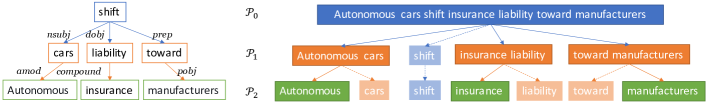
Figure 2: Dependency tree (left) by SpaCy Honnibal and Montani (2017) and recursive phrase partitions (right)

For sentence $s=[t_{1},...,t_{n}]$ containing $n$ tokens $t_{i},1\leq i\leq n$, we define the Recursive Phrase Partitions (RPP) as a set of partitions $\{\mathcal{P}_{0},\mathcal{P}_{1},...,\mathcal{P}_{L}\}$ of the sentence $s$, where $\mathcal{P}_{l}$ is the partition at $l$-th level, $1\leq l\leq L$. Specifically, $\mathcal{P}_{l}=[P_{l,1},...,P_{l,q}]$ contains a sequence of phrases, where the $q$-th phrase $P_{l,q}=s[b_{l,q}:e_{l,q}]$ is the span in $s$ from the beginning index $b_{l,q}$ to the ending index $e_{l,q}$. So we have two properties:

1. Concatenating all phrases recovers the sentence, that is $\oplus_{q}P_{l,q}=s$, where $\oplus$ is the string concatenation.

2. For two different levels, i.e. $0\leq l_{1}<l_{2}$, any phrase in level $l_{2}$ is contained in the unique phrase in level $l_{1}$.

In our definition, the $\mathcal{P}_{0}=[s]$ and $\mathcal{P}_{L}=[t_{1},..,t_{n}]$ are the coarsest partition and the finest partition, respectively. The second property guarantees that the recursive phrase partitions can be nested so that each phrase can be recursively divided. RPP can be constructed from any tree representation of the sentence, including constituency tree, dependency tree, or even naive binary separation of token sequences. Figure 2 shows an example of RPP from a dependency tree. Some phrases (such as ‘shift’ in $\mathcal{P}_{2}$) are added to satisfy the first property.

4.2 Compositional Phrase Semantics

Once the RPP structure of a sentence is given, we define the vector $\tilde{v}$ and weight $\tilde{w}$ for each phrase. Our definition is invariant with respect to the AC sentence embedding, that is, AC sentence embedding $x$ is invariant to the phrase partition $\mathcal{P}_{l}$ of the sentence.

$$x =\sum_{i}^{n}w_{i}v_{i}=\sum_{q}\tilde{w}_{l,q}\tilde{v}_{l,q},$$ (12)

where the phrase weights and vectors are given by

$$\tilde{w}_{l,q}=\sum_{i=b_{l,q}}^{e_{l,q}}w_{i},\tilde{v}_{l,q}=\sum_{i=b_{l,q}}^{e_{l,q}}w_{i}v_{i}/\tilde{w}_{l,q}.$$ (13)

In this way, the sentence vector can also be represented by the additive composition of phrase vectors and weights, where each phrase vector can be again composed by the word vectors additively. Our definitions of phrase weights and vectors recursively aggregate the information from finer-grained level (i.e. ‘autonomous’ and ‘cars’) information to coarser-grained level (i.e. ‘autonomous cars’). Furthermore, our discussion about EC similarity in Section 3.2 at the word level can also be generalized to any phrase partitions. That is, we can use the EC similarity to consider the inter-sentence phrase alignment and then correct the intra-sentence phrase semantics of each partition.

5 Recursive Optimal Transport and STS

In this section, we connect the dots by applying EC similarity in Section 3.2 to phrase alignment in Section 4 on tree structures. Specifically, we present Recursive Optimal Transport Similarity (ROTS) which computes the phrase alignment at each $(l+1)$-th level phrase partition with the guidance of the phrase alignment at the $l$-th level.

5.1 Prior Optimal Transport (Prior OT)

Prior OT Zhao et al. (2020) was firstly proposed to pass prior information when minimizing the entropy-regularized Wasserstein loss. When it comes to the OT-based STS, we re-consider the objective function in Problem (1) with an additional prior alignment $\Pi$:

$$~{}\sum_{ij}\Gamma_{ij}D_{ij}+\epsilon\mathrm{KL}(\Gamma\|\Pi),$$ (14)

where $\mathrm{KL}(\Gamma\|\Pi)=-\sum_{ij}\Gamma_{ij}\log{\Pi_{ij}}-H(\Gamma)$ is the KL-divergence between the phrase alignment $\Gamma$ and the prior alignment $\Pi$, and $H(\cdot)$ is the entropy. $\epsilon$ is the hyper-parameter that controls how close the obtained $\Gamma^{*}$ is to $\Pi$. When $\epsilon=0$, Equation (14) falls back to Equation (1), and when $\epsilon$ is sufficiently large, the optimal $\Gamma^{*}$ is sufficiently close to $\Pi$ in terms of KL-divergence.

Notably, the objective in Equation (14) can be minimized by the Sinkhorn algorithm Cuturi (2013); Zhao et al. (2020). Compared to tree kernels Moschitti (2006); Croce et al. (2011); Le et al. (2018), Sinkhorn algorithm is based on matrix operations such that it can be accelerated by GPUs Cuturi (2013). Sinkhorn algorithm has time complexity $O(mn/\epsilon^{2})$ Dvurechensky et al. (2018). In our practice, we usually choose the large prior strength, i.e. $\epsilon>1$ that allows faster convergence.

We can interpolate WRD and AC with the help of Prior OT under EC similarity.

Example 1 (EC Interpolation of WRD and AC).

Given a prior matrix $\Pi=\Gamma_{AC}$, we first compute the alignment $\Gamma_{\epsilon}$ by minimizing Equation (14) with WRD’s choice of $D,\mu,\nu$ in Equation (3). Then we compute the EC interpolation similarity by

$$\mathrm{Interp}=\tilde{C}\sum_{ij}\Gamma_{\epsilon,ij}\cos(v^{(1)}_{i},v^{(2)}_{j}),$$ (15)

where $\epsilon>0$ is the prior strength in Equation (14). When $(\alpha,\epsilon)=(0,0)$, $1-\mathrm{Interp}=s_{OT}$ . When $(\alpha,\epsilon)=(1,+\infty)$ , $\mathrm{Interp}=s_{AC}$.

5.2 Recursive Optimal Transport Similarity

Given two sentences $s^{(1)},s^{(2)}$ with their RPPs $\{\mathcal{P}^{(1)}_{0},\mathcal{P}^{(1)}_{1},...,\mathcal{P}^{(1)}_{L_{1}}\}$ and $\{\mathcal{P}^{(2)}_{0},\mathcal{P}^{(2)}_{1},...,\mathcal{P}^{(2)}_{L_{2}}\}$, ROTS considers partition pairs $(\mathcal{P}^{(1)}_{k},\mathcal{P}^{(2)}_{k})$ from the coarsest $k=0$ level to the finest $k=d\leq\min(L_{1},L_{2})$ level, where $d$ is a hyper-parameter. Given the computed $k$-th alignment matrix $\Gamma^{(k)}$ of $(\mathcal{P}^{(1)}_{k},\mathcal{P}^{(2)}_{k})$, ROTS constructs the following prior alignment $\Pi^{(k+1)}$ for next EC computation $(\mathcal{P}^{(1)}_{k+1},\mathcal{P}^{(2)}_{k+1})$.

$$\Pi^{(k+1)}_{m_{i}n_{j}}=\frac{\mu_{k+1,m_{i}}\nu_{k+1,n_{j}}\Gamma^{(k)}_{ij}}{\sum_{\tilde{m}_{i}\in P^{(1)}_{k,i},\tilde{n}_{j}\in P^{(2)}_{k,j}}\mu_{k+1,\tilde{m}_{i}}\nu_{k+1,\tilde{n}_{j}}}.$$ (16)

Specifically, the $(i,j)$ phrase alignment score $\Gamma_{ij}^{(k)}$ at $k$-th level will be separated to the sub-phrase alignment $(m_{i},n_{j})$ at the $(k+1)$-th level according to the marginal $\mu_{k+1,m_{i}}$ and $\nu_{k+1,n_{j}}$, where $m_{i},n_{j}$ are the index of the sub-phrase of $i,j$ respectively. With the coarse-to-fine prior $\Pi^{(k+1)}$, ROTS computes the phrase alignment matrix $\Gamma^{(k+1)}$ at the $(k+1)$-th level by Prior OT (Equation (14)). The computation process of ROTS is shown in Algorithm 1. For $k=0$, each sentence has a single vector, the alignment matrix $\Gamma^{(0)}=1$ is a $1\times 1$ matrix. The complexity of ROTS is $O(m+n+d(\rho^{d}/\epsilon)^{2})$ where $\rho$ is the maximum branching number of the tree and is usually small for natural language. When the hyper-parameter $d$ is fixed, the complexity of Algorithm 1 grows linearly with the sentence length $m$ and $n$ (see Table 1).

Our ROTS is featured by finding the finer-level phrase alignment under the guidance of the coarser-level phrase alignment. Unlike the tree kernels Le et al. (2018) that highly rely on syntax trees and syntax labels, ROTS is based on the EC phrase alignment at different phrase partition levels that are induced by a syntax tree. Specifically, the phrase alignments are obtained from the phrase semantic information, i.e. weights and vectors rather than plain syntax labels (see Table 1).

Algorithm 1 Recursive OT Similarity

0:  Two sentences $s^{(1)},s^{(2)}$ with recursive phrase partitions $\{\mathcal{P}^{(1)}_{0},\mathcal{P}^{(1)}_{1},...\}$ and $\{\mathcal{P}^{(2)}_{0},\mathcal{P}^{(2)}_{1},...\}$, depth $d$ and prior strengths $\epsilon_{k},k=1,...,d$, correction strength $\alpha$.

0:  $\mathrm{ROTS}_{k}$ at each level $k$.

1:  Prepare the weights and vectors at level $0$.

2:  Initialize 0-th level alignment $\Gamma^{(0)}\leftarrow 1$.

3:  for $k\leftarrow 1,...,d$ do

4:     Prepare the weights and vectors at level $k$.

5:     Get $k$-th prior $\Pi^{(k)}$ by Eq. (16) from $\Gamma^{(k-1)}$.

6:     Get $k$-th alignment $\Gamma^{(k)}$ by Eq. (14) with $\epsilon_{k}$.

7:     Get $\mathrm{ROTS}_{k}$ by Eq. (11) with $\tilde{C}=\alpha C+1-\alpha$, where $C=\frac{\sum_{k}w^{(2)}_{k}\lVert v^{(2)}_{k}\rVert}{\lVert\sum_{k}w^{(2)}_{k}v^{(2)}_{k}\rVert}\frac{\sum_{k}w^{(1)}_{k}\lVert v^{(1)}_{k}\rVert}{\lVert\sum_{k}w^{(1)}_{k}v^{(1)}_{k}\rVert}$.

8:  end for

6 Experiments

We first present the experimental setting of unsupervised STS. Then we conduct the benchmark study of all unsupervised STS approaches. Detailed ablation studies justify the effect of ROTS. In the appendix, further discussions on the impact of word vectors, and preprocessing steps are included.

6.1 Experimental Settings

Text processing SpaCy Honnibal and Montani (2017) is a open-source text processing toolkit including rich functionality such as tokenization and dependency parsing. It is very suitable for preprocessing pipelines. The text processing model in en_core_web_sm is used.

Word vectors Word2Vec Mikolov et al. (2013), GloVe Pennington et al. (2014), and fastText Bojanowski et al. (2017) are considered in the unsupervised STS cases. Two word vectors trained on transferred learning settings, i.e. PSL Wieting et al. (2015) and ParaNMT Wieting and Gimpel (2018), are considered in the transferred STS cases. Further information can be found in Appendix A.2.

Preprocessing The scope of our pre-processing steps extends the “vector converters” in Yokoi et al. (2020). Those preprocessing steps can all be applied to EC similarity and are detailed in Appendix A.3. Three typical setups are selected, including SUP Ethayarajh (2018), SWC Yokoi et al. (2020) and WR Arora et al. (2017).

Datasets We consider (1) STSB dev and test set in STS-Benchmark Cer et al. (2017); (2) STS[year] STS from 2012 to 2016 Agirre et al. (2012, 2013, 2014, 2015, 2016); (3) SICK Marelli et al. (2014); (4) Twitter Xu et al. (2015). Details can be found in Appendix A.1. Each dataset includes several sub-tasks, and there are 29 tasks in total.

Related baselines Some unsupervised STS baselines are closely related to EC similarity, including COS (SIF Arora et al. (2017), uSIF Ethayarajh (2018)), ACV-Tree Le et al. (2018), and WRD Yokoi et al. (2020). WMD Kusner et al. (2015) is important but not included since WMD has been shown clearly suboptimal to WRD Yokoi et al. (2020).

Other Unsupervised Baselines BERT’s final-layer and last-2-layers embeddings (BERT and BERT-last2ave) Li et al. (2020) BERTScore Zhang et al. (2020), DynaMax-Jaccard Zhelezniak et al. (2019a), Center Kernel Alignment (CKA) Zhelezniak et al. (2019b) and Kraskov-Stögbauer–Grassberger Kraskov et al. (2004) (KSG) cross entropy estimation Zhelezniak et al. (2020).

Default hyper-parameters We summarize the result with different parameters. Results show that excellent scores are achieved with $\alpha=1$, $d=4$ and $\epsilon_{k}=10,1\leq k\leq L$.

6.2 Unsupervised Benchmark

An unsupervised STS benchmark study is conducted over STSB, SICK, and STS by years (STS12-16). Twitter is not included since most of the baselines did not report the score. fastText is chosen as the pretrained word vector.

Table 2: Pearson’s $r\times 100$ for ROTS and related unsupervised baselines. Best cases are in boldface.

Similarity	STSB	SICK	STS12	STS13	STS14	STS15	STS16
ACV-Tree Le et al. (2018)	-	-	61.60	-	72.83	75.80	-
BERTScore fastText Zhang et al. (2020)	53.86	64.69	51.95	45.86	61.66	69.00	-
SIFArora et al. (2017)	70.13	73.20	63.46	59.30	72.95	73.27	70.79
uSIFEthayarajh (2018)	73.47	72.73	63.24	61.41	74.37	76.33	73.47
WRD+SWCYokoi et al. (2020)	74.58	67.09	63.80	57.55	71.06	77.65	75.46
WRD+SUPYokoi et al. (2020)	74.80	67.67	64.03	58.50	71.32	77.65	75.38
WRD+WRYokoi et al. (2020)	73.13	68.73	63.81	58.09	70.60	77.28	74.48
ROTS+SWC+mean	75.33	71.79	63.91	62.29	74.30	77.96	75.95
ROTS+SUP+mean	74.25	73.13	63.52	61.49	74.44	76.75	74.28
ROTS+WR+mean	71.52	73.84	63.77	59.58	73.15	73.91	71.97

Table 3: Spearman’s $\rho\times 100$ for ROTS and other unsupervised baselines. Best cases are in boldface.

Similarity	STSB	SICK	STS12	STS13	STS14	STS15	STS16
$\mathrm{BERT}_{\mathrm{large}}$ Devlin et al. (2019)	46.99	53.74	46.89	53.32	49.27	56.54	61.63
$\mathrm{BERT}_{\mathrm{large}}$-last2avg Li et al. (2020)	59.56	60.22	57.68	61.37	61.02	68.04	70.32
KSG k=10 Zhelezniak et al. (2020)	-	-	60.40	61.50	68.30	77.00	75.10
MaxPool+KSG k=10 Zhelezniak et al. (2020)	-	-	59.50	60.20	67.50	75.00	74.10
DynaMax Jaccard Zhelezniak et al. (2019a)	-	-	61.30	61.70	66.90	76.50	74.70
CKA dCorr Zhelezniak et al. (2019b)	-	-	60.90	63.40	67.80	76.20	73.40
CKA Gaussian Zhelezniak et al. (2019b)	-	-	60.80	64.60	68.00	76.40	73.80
ROTS+SWC+mean	72.69	62.88	63.07	62.61	70.73	78.06	75.74
ROTS+SUP+mean	71.63	61.81	62.13	61.04	70.85	77.26	74.50
ROTS+WR+mean	69.78	61.39	61.48	59.29	70.19	75.18	73.26

We re-implement SIF, uSIF and WRD and compare the Pearson’s $r\times 100$ in Table 2 together with the ACV-Tree and BERTScore+fastText. Other baselines are compared by Spearman’s $\rho$ in Table 3. The clear advantage of ROTS-mean is shown. Our results confirm the finding reported by Yokoi et al. (2020) that the BERT-based method is sub-optimal under unsupervised settings.

6.3 Ablation Study

For ablation study, the scores are averaged from scores on the three datasets, including SICK, STSB test, and Twitter. We don’t include STS12-16 since they overlap with STSB. Depths and Aggregations, Correction and Prior, and Recursive Phrase Partitions are discussed since they are closely related to ROTS. More experiments on different word vectors and preprocessings can be found in Appendix B. Uncertainty quantification by the BCa confidence interval Efron (1987) on different datasets can be found in Appendix E.

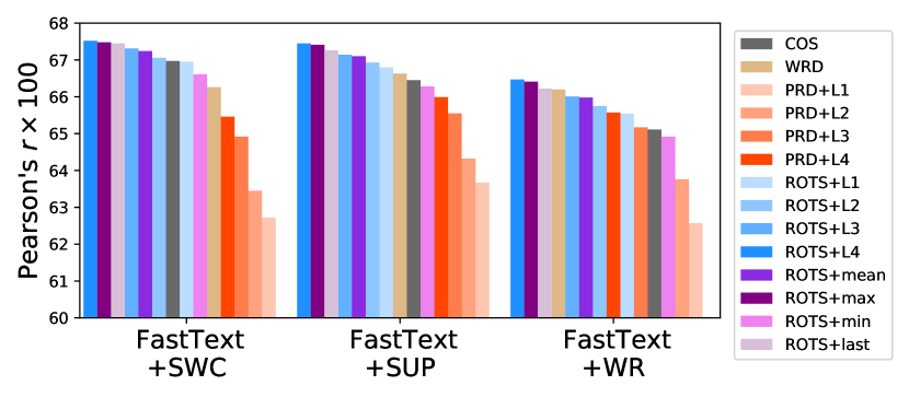
Figure 3: Ablation study for ROTS depth and aggregation. Scores are averaged from STSB, Twitter and SICK.

Depths and Aggregations

Once all $\mathrm{ROTS}_{k}$ are obtained, we consider different aggregation methods including mean, max, min, last and picks the $k$-th level. The ablation study of depth and aggregation is shown in Figure 3. We report the ROTS results at different levels and different aggregations. We also include the Phrase Rotator’s Distance (PRD) at the same recursive phrase partitions as ROTS. PRD-L$k$ is the special case of ROTS-L$k$ by setting $\epsilon_{k}=0$ and $\alpha=0$. AC is equivalent to 0-th level ROTS and WRD is the L-th level of PRD so they are included.

ROTS similarities (blue and purple bars) dominate among all other baselines. We can see that the performances of ROTS and PRD increase as their levels get deeper (the related bars are plotted with deeper blue and orange colors). Interestingly, PRDs are generally worse than WRD, which indicates that the naive phrase alignment may not be suitable, and may suffer from sub-optimal inter-sentence alignment and intra-sentence semantics. The performance gains of ROTS-L$k$ from PRD-L$k$ clearly show that both the coarse-to-fine prior and the EC similarity are important.

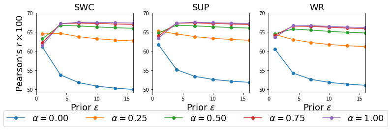
Figure 4: Effects of correction and prior for ROTS-L4 on fastText vectors

Correction Step and Prior

We adjust the $\alpha$ in Definition 1 to control the correction effect and the $\epsilon_{k}$ for the prior strength at the $k$-th phrase partition level. For simplicity, we assume prior strengths $\epsilon_{k}$ are controlled by the single parameter $\epsilon$. We report the Pearson’s $r\times 100$ of ROTS-L4 averaged on the three datasets in Figure 4 since ROTS-L4 is the best in Figure 3. As shown in Figure 4, proper correction and prior are essential to produce good performances. The correction step is very important since results without it decrease significantly. This is consistent with the PRD observation in Figure 3. $\alpha$ and $\epsilon$ can be chosen easily since the performances is good and consistent if $\alpha>0.5$ and $\epsilon>5$.

Recursive Phrase Partitions

ROTS relies on the recursive phrase partitions that might be produced from parsing trees. Instead of exhausting the parsers, we consider the simplest binary tree, i.e. the sub-phrase partition is constructed by uniformly splitting each phrase, to show the lower bound of the ROTS performances. We see from Table 4 that the ROTS with spaCy dependency parser performs best in all cases among related baselines. Given the preprocessing setups, we find that the binary tree still outperforms WRD and AC with SUP and SWC setups. For sub-optimal WR setup, ROTS with the binary tree are very close to that in WRD and better than AC. Though preprocessing setups affect the performance, we can observe the performance gain by introducing the recursive phrase partitions given the setup. Therefore, we conclude that the coarse-to-fine prior captures the intra-sentence structures. The performance gain can be observed by even the simplest binary tree.

6.4 More empirical experiments

Some results are presented in the Appendix, including the justification of more choices on preprocessing in Appendix B.2, comparison under transfer and supervised setting in Appendix B.3, computation time in Appendix C, interpolation of WRD and AC by EC similarity in Appendix D.

Table 4: Pearson’s $r\times 100$ for different parsers. spaCy: ROTS-L4 with the spaCy parser, Binary: ROTS-L4 with a binary tree. The best score is indicated in the boldface and the second highest score is underlined.

Model	spaCy	Binary	WRD	AC
fastText + SUP	67.45	67.20	66.63	66.45
fastText + SWC	67.52	67.26	66.26	66.97
fastText + WR	66.47	66.15	66.20	65.11

7 Conclusion

In this paper, we present a new EC similarity of STS that allows flexible adaptation of word-level alignment, which successfully unifies three different unsupervised approaches. By taking advantage of the recursive phrase partitions, we generalize EC similarity to the phrase alignment. Then, we propose ROTS, a new sentence similarity that considers phrase semantics by conducting phrase alignment in a coarse-to-fine order under the coarse-to-fine prior OT. The thorough comparison with unsupervised baselines demonstrates the state-of-the-art performance and technical details of ROTS are fully justified by the ablation study.

8 Acknowledgement

This work was supported by the National Key R&D Program of China (2020AAA0109603).

Appendix A Extended Experimental Setup information

A.1 Dataset details

• STSB dev and test set in STS-Benchmark Cer et al. (2017). It can be downloaded directly from Ethayarajh (2018)’s implementation .

• STS[year] STS from 2012 to 2016 Agirre et al. (2012, 2013, 2014, 2015, 2016). STS12 contains 5 subtasks, STS13 contains 4 subtasks, STS14 contains 6 subtasks, STS15 contains 5 subtasks and STS16 contains 5 subtasks. The reported score is averaged from scores for related subtasks. It can be obtained by Conneau and Kiela (2018)’s implementation . A newer implementation is also available .

• SICK Semantic relatedness task at SemEval 2014 Marelli et al. (2014). It can be downloaded directly from Ethayarajh (2018)’s implementation .

• Twitter Paraphrase and semantic similarity in Twitter (PIT) at SemEval 2015 Xu et al. (2015). This dataset was obtained by emailing the author.

A.2 Pretrained Word Vectors

We list the downloadable links of word vectors used in this paper.

• Word2Vec Mikolov et al. (2013): We use the pretrained word2vec . However, this file is in .bin format. We use gensim Řehůřek and Sojka (2010) to convert the file to .vec format.

• GloVe Pennington et al. (2014): We use the 300D GloVe vectors trained on Common Crawl (840B tokens, 2.2M vocabulary) .

• fastText Bojanowski et al. (2017): We use the 300D fastText vectors trained on Common Crawl (600B tokens) without subword information .

• PSL Wieting et al. (2015): We use the pretrained vectors from the author .

• ParaNMT Wieting and Gimpel (2018): Two versions are provided by the author  and we keep the same choice as  Ethayarajh (2018) .

A.3 Preprocessing of word vectors

Other preprocessing setups are discussed as follows: Here we list several preprocessing approaches mentioned in previous research. For those with hyper-parameters, we also give the hyper-parameters used in this paper.

• Word-level Each word is associated with one weight. We consider SIF (W)eights Arora et al. (2017) with $a=10^{-3}$ and (U)SIF weights Ethayarajh (2018).

• Vocabulary-level Vectors are modified based on the vectors of words in the whole vocabulary, e.g. (A)ll-but-the-top Mu and Viswanath (2018) with $D=3$, (C)onceptor negation Liu et al. (2019) with $\alpha=2$.

• Sentence-level Vectors are modified by vectors of words in the same sentence, including Dimension-wise (S)caling Ethayarajh (2018).

• Corpus-level Vectors are modified based on all sentences in the corpus, e.g. main component (R)emoval Arora et al. (2017) and (P)iece-wise component removal Ethayarajh (2018) with $p=5$.

Table 5: Necessary resources of typical STS model

Model	Pretrain				Data
	Parser	Weights	Word Vector	Language Model	Training texts	Training labels	Transferred texts	Transferred labels
Unsupervised setting
BERT layer embedding Devlin et al. (2019)	✗	✗	✗	✓	✗	✗	✗	✗
BERTScore Zhang et al. (2020)	✗	✗	✗	✓	✗	✗	✗	✗
Additive composition Arora et al. (2017); Ethayarajh (2018)	✗	✓	✓	✗	✗	✗	✗	✗
DynaMax-Jaccard Zhelezniak et al. (2019a)	✗	✓	✓	✗	✗	✗	✗	✗
Center Kernel Alignment Zhelezniak et al. (2019b)	✗	✓	✓	✗	✗	✗	✗	✗
KSG cross entropy Zhelezniak et al. (2020)	✗	✓	✓	✗	✗	✗	✗	✗
OT Kusner et al. (2015); Yokoi et al. (2020)	✗	✓	✓	✗	✗	✗	✗	✗
ACV-Tree Le et al. (2018)	✓	✓	✓	✗	✗	✗	✗	✗
ROTS (ours)	✓	✓	✓	✗	✗	✗	✗	✗
Transfer and domain adaptation settings
SentenceBERT Reimers and Gurevych (2019)	✗	✗	✗	✓	✗	✗	*NLI	*NLI
BERT-Flow-*NLI Li et al. (2020)	✗	✗	✗	✓	✗	✗	*NLI	✗
BERT-Flow-*target Li et al. (2020)	✗	✗	✗	✓	✓	✗	✗	✗
SimCSE-*NLI Gao et al. (2021)	✗	✗	✗	✓	✗	✗	*NLI	*NLI
Fine-tuning LM
BERT-Finetune	✗	✗	✗	✓	✓	✓	✗	✗

A.4 Various STS and the required resources

We summarize the usage of data and other resources of popular STS models in Table 5. The key difference between unsupervised settings and other settings is the usage of external data to further train the model. We majorly consider the approaches that can be used without training.

Appendix B Extended Experiments

B.1 Joint effect of word vectors and preprocessings

We investigate the effects of the word vectors in Table 6. It has been shown that fastText is the best word vector for all three kinds of unsupervised STS regardless of the three pre-processing steps. Furthermore, ROTS performs best compared to AC and WRD when the fastText is chosen.

Table 6: Pearson’s $r\times 100$ for benchmark study with different word vectors and pre-processing setups. The best word vector achieved given the same pre-processing setup is indicated by boldface. The best pre-processing setup given the word vector is underlined.

Pre-processing	Word Vectors	Similarity
		AC	WRD	ROTS
WR	fastText	65.11	66.20	66.47
	GloVe	57.86	61.92	60.73
	Word2Vec	57.35	59.52	58.68
SWC	fastText	66.97	66.26	67.52
	GloVe	66.57	65.21	66.95
	Word2Vec	60.21	60.13	60.66
SUP	fastText	66.45	66.63	67.45
	GloVe	64.08	65.04	65.53
	Word2Vec	57.69	59.49	58.90

B.2 Other preprocessing setups

In Table 6, it is also found that SWC is the best performed pre-processing setup in eight out of nine combinations of word vectors and unsupervised STSes. It is also shown that given the SWC as the preprocessing setup, ROTS performs best among three unsupervised STS for all three kinds of word vectors. We also explore the combination of preprocessing setups from word level to corpus level. We provide preliminary results about the impact of preprocessing on ROTS in STSB test split with fastText vectors. We report the score of ROTS-L4 in Table 7.

Table 7: STSB test results by ROTS-L4 with fastText vectors with different preprocessing setups.

Setup	Pearson’s $r\times 100$	BCa 95% CI
+W	72.59	[70.02, 74.90]
+WR∗	72.34	[69.81, 74.66]
+U	72.62	[70.01, 74.96]
+SU	74.52	[71.90, 76.89]
+SUP∗	74.69	[72.01, 77.00]
+SW	74.78	[72.31, 77.11]
+SWP	74.90	[72.32, 77.08]
+SWA	74.97	[72.47, 77.15]
+SUA	75.20	[72.73, 77.43]
+SWR	75.21	[72.75, 77.45]
+SUR	75.35	[72.88, 77.53]
+SWC∗	75.66	[73.23, 77.84]
+SUC	75.73	[73.25, 77.95]
+SWRC	75.80	[73.33, 77.92]
+SWRCA	75.86	[73.46, 78.11]
+SURC	75.89	[73.39, 78.08]
+SURCA	75.94	[73.49, 78.18]

By Table 7, we suggest that C at the vocabulary level, S at the sentence level, R at the corpus level are beneficial. It is not clear which one of U or W in the word level for ROTS-L4 is more effective. As a result, we propose to combine the choices for vocabulary, sentence, and corpus levels, i.e. SCR for ROTS with U or W. Moreover, we think the two preprocessing setups in the vocabulary level, i.e. CA can also be combined. The best performance of ROTS-L4 is achieved by SURCA. The setups suggested by previous words are starred in the table, i.e. SWC for WRD Yokoi et al. (2020), SUP Ethayarajh (2018) and WR Arora et al. (2017) for AC. Though they may not be the best choice for ROTS-L4, we argue the results presented are sufficient to reveal the advantage of ROTS over other related baselines under various setups.

Table 8: Spearman’s $\rho\times 100$ for different models in semisupervised and transferred setting

Similarity	STS-B	SICK	STS12	STS13	STS14	STS15	STS16
ParaNMT Transfer
ROTS+WR+mean (ParaNMT)	78.51	65.90	65.39	63.95	75.41	79.90	77.86
ROTS+SWC+mean (ParaNMT)	78.65	65.29	64.88	62.08	74.24	79.16	76.38
SNLI + MNLI transfer
Sentence BERT(large)	79.23	73.75	72.27	78.46	74.90	80.99	76.25
Sentence RoBERTa(large)	79.10	74.29	74.53	77.00	73.18	81.85	76.82
domain adaptation setting
BERT (large) Flow *NLI	68.09	64.62	61.72	66.05	66.34	74.87	74.47
BERT (large) Flow target	72.26	62.50	65.20	73.39	69.42	74.92	77.63
SimCSE-BERT *NLI	76.85	72.23	68.40	82.41	74.38	80.91	78.56

B.3 Evaluation for transfer and semi-supervised settings

The results can be found in Table 8. ROTS that using the transferred ParaNMT word vector has good performance even compared to Sentence BERT with pretrained BERT large or RoBERTa large Reimers and Gurevych (2019), and is better than the domain adaptation settings Li et al. (2020). It is shown that PLM based models Cer et al. (2018); Reimers and Gurevych (2019); Li et al. (2020); Gao et al. (2021) are on par with ROTS with transfered word vectors Wieting and Gimpel (2018).

Appendix C Computation Speed

We report the computation speed for different similarities on a computer with an Intel i7 CPU of 2.6 GHz with 6 cores and 16 GB RAM. The optimal transport is computed by the POT Flamary et al. (2021) package .

We compare the computation of ROTS with WRD and PRD on STS-B test split (1379 sentence pairs to compute in total). Notably, we focus on the speed by Sinkhorn algorithm Cuturi (2013) for two reasons: (1) it has $O(n^{2})$ time complexity; (2) it can be easily accelerated by GPU.

Table 9 reports the speed by different OT-based algorithms. We note that the reported speeds for phrase alignment algorithms (PRD and ROTS) also include the time for parsing and constructing the recursive phrase partitions. This additional process brings additional computational overhead and slows down the speed. As a consequence of parsing, we can see that for PRD, #OT/sec is slowed down compared to WRD. However, ROTS is based on Prior OT with larger regularization strength, and each call of ot.sinkhorn requires much less time, thus making up the computational overhead by parsing.

Table 9: Comparison of computation speed

Method	Function in POT	Reg	Reg. Strength	#OT/STS	#STS/sec	#OT/sec
WRD	ot.sinkhorn	Entropy	0.1	1	208.52	208.52
PRD 4 levels	ot.sinkhorn	Entropy	0.1	5	32.80	164.00
ROTS 4 levels	ot.sinkhorn	KL Prior	10	5	60.56	302.80

Appendix D EC Interpolation of WRD and AC

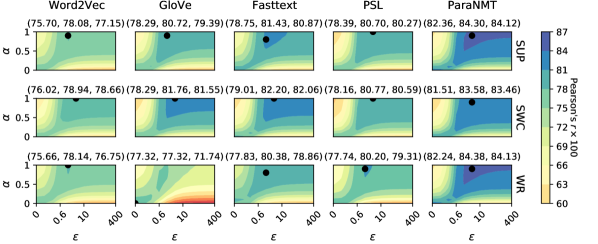
Figure 5: Interpolating AC and WRD by Example 1 on STS-B dev set. For each case, black dots indicate the highest score. The title of each subplot indicates scores by (WRD, Best Interpolation, AC).

We consider 15 combinations from 5-word vectors and 3 preprocessing setups. For each case, we grid-search 10 values of $\alpha$ by linearly splitting $[0,1]$, and 10 values of $\epsilon$ by logarithmically splitting $[0,400]$, resulting in 100 runs. The performances of 15 cases are shown in Figure 5. Grid-search results indicate that the proper choice of EC similarity outperforms both WRD and AC, thus showing solidness. Specifically, most of the best interpolation performances appear when $\alpha=1$ (14 cases) and $\epsilon\in[1,10]$ (14 cases), which confirms the ablation study in Figure 4. This observation demonstrates the effectiveness of the correction term and indicates that the best choice of the alignment matrix should be chosen carefully.

Appendix E Dataset Breakdown Tables and Uncentity Quantification

We provide the breakdown tables related to Figure 3 with different word vectors, e.g. fastText in Table 13, GloVe in Table 14, Word2Vec in Table 15, PSL in Table 16 and ParaNMT in Table 17. We see that WRD performs consistently well on Twitter dataset. For STSB and SICK, ROTS is better, resulting in the best overall performance.

E.1 Three Typical Preprocessings

We provide further information for Table 2, including the Pearson’s $r\times 100$ for each individual datasets, plus STSB dev split and Twitter. Still, we focus on fastText vectors, and list three preprocessing setups, e.g. WR in Table 10, SWC in Table 11, SUP in Table 12. We find that ROTS has the best performance in WR and SUP, which is consistent with Table 2, and AC is good with SWC.

Table 10: Breakdown table for benchmark study with WR preprocessing

dataset	subsplit/subtask	AC		WRD		ROTS
		Pearson’s $r\times 100$	BCa 95% CI	Pearson’s $r\times 100$	BCa 95% CI	Pearson’s $r\times 100$	BCa 95% CI
STSB	test	70.13	[67.35, 72.53]	73.13	[70.40, 75.54]	72.34	[69.78, 74.66]
	dev	78.85	[76.93, 80.56]	77.83	[75.49, 79.87]	79.78	[77.76, 81.48]
Twitter	test	52.01	[47.67, 56.15]	56.73	[52.07, 60.83]	53.32	[48.75, 57.45]
SICK	test	73.20	[71.66, 74.68]	68.73	[67.13, 70.27]	73.75	[72.16, 75.17]
STS12	MSRpar	39.84	[33.68, 45.44]	49.93	[44.04, 54.97]	43.04	[36.93, 48.40]
	MSRvid	86.01	[84.22, 87.59]	82.38	[79.82, 84.57]	86.35	[84.59, 87.91]
	SMTeuroparl	52.41	[44.52, 60.64]	52.01	[45.61, 58.37]	51.95	[44.82, 59.52]
	OnWN	74.31	[70.55, 77.55]	74.59	[71.42, 77.30]	74.43	[70.78, 77.58]
	SMTnews	64.71	[54.76, 73.79]	60.13	[52.37, 67.16]	62.92	[53.37, 72.18]
STS13	FNWN	42.94	[29.66, 53.80]	48.59	[35.52, 58.61]	44.64	[31.36, 55.42]
	headlines	72.88	[69.45, 75.99]	72.49	[68.53, 75.73]	73.52	[69.99, 76.54]
	OnWN	82.36	[79.81, 84.57]	69.74	[65.22, 73.64]	80.67	[77.85, 83.07]
	SMT	39.03	[31.69, 46.65]	41.56	[34.95, 47.44]	40.65	[33.25, 47.89]
STS14	deft-forum	51.99	[45.09, 58.05]	46.53	[38.71, 53.75]	50.78	[43.96, 56.97]
	deft-news	74.54	[68.55, 78.93]	74.62	[68.82, 79.55]	75.52	[69.80, 79.83]
	headlines	68.71	[64.55, 72.33]	67.29	[62.68, 71.45]	69.27	[65.17, 73.02]
	OnWN	84.52	[82.31, 86.32]	76.45	[73.25, 79.17]	83.62	[81.32, 85.56]
	images	81.33	[78.78, 83.43]	80.06	[77.09, 82.50]	81.72	[79.20, 83.82]
	tweet-news	76.62	[72.87, 79.78]	78.65	[75.59, 81.33]	78.27	[74.88, 81.19]
STS15	answers-forums	70.51	[64.96, 75.13]	75.15	[70.11, 79.29]	71.86	[66.44, 76.29]
	answers-students	70.86	[66.85, 74.32]	76.02	[72.59, 79.00]	72.49	[68.70, 75.71]
	belief	68.88	[61.09, 74.18]	77.71	[71.39, 81.99]	70.61	[62.59, 75.62]
	headlines	74.44	[71.27, 77.11]	73.69	[70.17, 76.70]	74.79	[71.52, 77.53]
	images	81.68	[79.23, 83.74]	83.83	[81.28, 85.90]	83.17	[80.75, 85.13]
STS16	answer-answer	47.15	[37.71, 55.50]	60.61	[52.21, 67.26]	53.36	[44.49, 60.90]
	headlines	72.39	[66.12, 77.41]	73.41	[65.76, 79.02]	73.55	[67.06, 78.37]
	plagiarism	82.01	[77.92, 85.28]	82.46	[77.73, 86.24]	82.53	[78.53, 85.90]
	postediting	79.37	[71.53, 83.43]	86.11	[81.33, 89.16]	79.81	[72.99, 83.71]
	question-question	73.03	[66.30, 77.87]	69.79	[61.18, 76.30]	73.79	[67.24, 78.60]
MEAN		68.51	-	69.32	-	69.40	-

Table 11: Breakdown table for benchmark study with SWC preprocessing

dataset	subsplit/subtask	AC		WRD		ROTS
		Pearson’s $r\times 100$	BCa 95% CI	Pearson’s $r\times 100$	BCa 95% CI	Pearson’s $r\times 100$	BCa 95% CI
STSB	test	74.78	[72.31, 77.06]	74.58	[72.08, 76.81]	75.66	[73.17, 77.86]
	dev	82.06	[80.25, 83.67]	78.47	[76.27, 80.45]	81.33	[79.36, 83.08]
Twitter	test	54.01	[49.35, 58.23]	57.10	[52.42, 61.23]	55.56	[50.95, 59.88]
SICK	test	72.12	[70.63, 73.57]	67.09	[65.49, 68.60]	71.33	[69.80, 72.76]
STS12	MSRpar	52.05	[46.24, 57.40]	54.85	[49.29, 59.92]	51.96	[46.18, 57.32]
	MSRvid	87.23	[85.39, 88.76]	80.91	[78.23, 83.20]	85.48	[83.36, 87.22]
	SMTeuroparl	55.44	[49.45, 61.30]	52.75	[46.66, 58.26]	52.94	[46.55, 59.00]
	OnWN	73.66	[69.82, 77.04]	73.80	[70.63, 76.62]	73.52	[69.84, 76.80]
	SMTnews	56.28	[47.71, 64.54]	56.68	[49.28, 63.64]	54.27	[46.13, 62.82]
STS13	FNWN	53.69	[41.93, 62.83]	47.98	[36.27, 57.19]	53.49	[41.82, 63.02]
	headlines	75.92	[72.66, 78.76]	73.67	[70.14, 76.79]	75.38	[71.92, 78.32]
	OnWN	82.89	[80.04, 85.20]	67.57	[62.91, 71.77]	76.66	[73.17, 79.70]
	SMT	41.81	[34.69, 48.45]	40.98	[34.52, 46.79]	42.44	[35.82, 48.50]
STS14	deft-forum	55.57	[48.68, 61.79]	48.98	[41.00, 55.68]	54.31	[47.11, 60.52]
	deft-news	75.92	[70.33, 80.46]	75.63	[70.18, 80.18]	76.13	[70.56, 80.70]
	headlines	71.27	[67.27, 74.83]	69.07	[64.70, 73.00]	71.13	[67.08, 74.74]
	OnWN	85.05	[82.85, 86.93]	75.28	[72.13, 78.04]	81.41	[78.77, 83.66]
	images	83.08	[80.47, 85.19]	79.24	[76.29, 81.77]	82.02	[79.39, 84.25]
	tweet-news	79.02	[75.83, 81.82]	78.16	[75.11, 80.76]	79.30	[76.24, 82.05]
STS15	answers-forums	75.46	[70.52, 79.33]	75.29	[70.37, 79.42]	75.76	[70.83, 79.78]
	answers-students	74.15	[70.73, 77.18]	76.29	[73.12, 79.10]	74.10	[70.68, 77.12]
	belief	78.22	[72.24, 82.23]	77.92	[72.15, 82.19]	78.56	[73.04, 82.59]
	headlines	77.10	[74.12, 79.68]	75.11	[71.84, 78.09]	76.73	[73.70, 79.52]
	images	85.48	[83.09, 87.40]	83.65	[80.95, 85.76]	85.39	[83.04, 87.25]
STS16	answer-answer	60.44	[51.81, 67.64]	63.92	[56.17, 70.26]	61.66	[53.52, 68.76]
	headlines	75.61	[68.93, 80.37]	75.28	[67.87, 80.65]	75.71	[68.87, 80.67]
	plagiarism	83.48	[79.25, 86.80]	81.55	[76.49, 85.31]	82.46	[77.98, 86.01]
	postediting	83.63	[77.69, 87.06]	86.90	[82.05, 89.85]	84.28	[78.84, 87.61]
	question-question	76.09	[68.65, 81.22]	69.66	[61.28, 76.39]	76.08	[68.90, 81.01]
MEAN		71.78	-	69.60	-	71.21	-

Table 12: Breakdown table for benchmark study with SUP preprocessing

dataset	subsplit/subtask	AC		WRD		ROTS
		Pearson’s $r\times 100$	BCa 95% CI	Pearson’s $r\times 100$	BCa 95% CI	Pearson’s $r\times 100$	BCa 95% CI
STSB	test	73.47	[70.90, 75.86]	74.80	[72.27, 77.13]	74.69	[72.12, 77.01]
	dev	80.87	[78.98, 82.55]	78.75	[76.54, 80.72]	81.15	[79.23, 82.92]
Twitter	test	53.15	[48.54, 57.23]	57.41	[52.87, 61.57]	54.88	[50.28, 59.08]
SICK	test	72.73	[71.16, 74.24]	67.67	[66.06, 69.17]	72.77	[71.26, 74.22]
STS12	MSRpar	41.40	[35.15, 46.68]	50.98	[45.25, 56.10]	44.77	[38.66, 50.10]
	MSRvid	86.79	[84.94, 88.35]	83.27	[80.83, 85.32]	87.04	[85.18, 88.62]
	SMTeuroparl	53.29	[46.42, 60.68]	52.73	[46.49, 58.45]	52.31	[45.42, 58.92]
	OnWN	73.53	[69.66, 76.91]	73.85	[70.76, 76.55]	73.56	[69.81, 76.79]
	SMTnews	61.19	[51.71, 70.15]	59.34	[52.19, 66.10]	59.92	[50.88, 69.08]
STS13	FNWN	49.52	[37.76, 59.05]	49.16	[37.65, 58.60]	50.25	[38.73, 59.72]
	headlines	73.73	[70.24, 76.79]	72.95	[69.30, 76.21]	74.11	[70.65, 77.17]
	OnWN	83.15	[80.48, 85.50]	71.12	[66.69, 74.82]	81.14	[78.13, 83.53]
	SMT	39.22	[32.18, 46.23]	40.78	[34.34, 46.68]	40.50	[33.48, 47.03]
STS14	deft-forum	53.39	[46.27, 59.71]	47.60	[39.96, 54.72]	52.21	[45.10, 58.70]
	deft-news	76.08	[70.28, 80.42]	75.38	[69.79, 80.11]	76.91	[71.41, 81.28]
	headlines	69.86	[65.85, 73.29]	68.11	[63.55, 72.19]	70.12	[65.97, 73.73]
	OnWN	85.37	[83.20, 87.16]	77.55	[74.59, 80.08]	84.05	[81.72, 85.98]
	images	83.73	[81.36, 85.71]	81.05	[78.26, 83.51]	83.65	[81.31, 85.67]
	tweet-news	77.78	[74.24, 80.79]	78.24	[75.16, 80.85]	78.86	[75.59, 81.61]
STS15	answers-forums	74.60	[69.78, 78.61]	75.80	[70.74, 79.72]	75.40	[70.34, 79.27]
	answers-students	70.66	[66.65, 74.13]	75.16	[71.79, 78.21]	72.18	[68.21, 75.47]
	belief	76.53	[70.16, 80.98]	78.37	[72.23, 82.48]	77.23	[70.94, 81.64]
	headlines	75.16	[72.06, 77.80]	74.28	[70.94, 77.36]	75.42	[72.23, 78.15]
	images	84.70	[82.47, 86.60]	84.66	[82.23, 86.64]	85.31	[83.12, 87.13]
STS16	answer-answer	54.75	[45.45, 62.55]	62.77	[54.87, 69.23]	58.21	[49.27, 65.50]
	headlines	72.71	[66.44, 77.66]	74.16	[66.53, 79.74]	73.90	[67.05, 78.90]
	plagiarism	82.37	[78.29, 85.55]	82.21	[77.61, 86.05]	82.62	[78.53, 85.92]
	postediting	82.64	[76.07, 86.31]	86.54	[81.65, 89.56]	83.08	[76.90, 86.66]
	question-question	74.91	[67.20, 79.98]	71.21	[63.00, 77.61]	75.57	[68.48, 80.59]
MEAN		70.25	-	69.86	-	70.75	-

E.2 Five Word Vectors

Table 13: Breakdown table with fastText vectors

Similarity	STSB		Twitter		SICK		MEAN
	Pearson’s $r\times 100$	BCa 95% CI	Pearson’s $r\times 100$	BCa 95% CI	Pearson’s $r\times 100$	BCa 95% CI	Pearson’s $r\times 100$
with SUP
WRD	74.80	[72.27, 77.13]	57.41	[52.87, 61.57]	67.67	[66.06, 69.17]	66.63
AC	73.47	[70.90, 75.86]	53.15	[48.54, 57.23]	72.73	[71.16, 74.24]	66.45
ROTS+L0	73.47	[70.77, 75.76]	53.15	[48.47, 57.13]	72.73	[71.19, 74.25]	66.45
ROTS+L1	73.77	[71.24, 76.08]	53.34	[48.84, 57.51]	73.31	[71.71, 74.74]	66.81
ROTS+L2	74.02	[71.40, 76.34]	53.40	[48.76, 57.63]	73.37	[71.85, 74.81]	66.93
ROTS+L3	74.05	[71.25, 76.44]	54.23	[49.76, 58.44]	73.13	[71.56, 74.58]	67.14
ROTS+L4	74.69	[72.12, 77.01]	54.88	[50.28, 59.08]	72.77	[71.26, 74.22]	67.45
ROTS+mean	74.25	[71.70, 76.56]	53.93	[49.50, 58.13]	73.13	[71.59, 74.58]	67.10
ROTS+max	74.58	[71.87, 76.86]	54.88	[50.39, 59.04]	72.77	[71.27, 74.23]	67.41
ROTS+min	73.36	[70.57, 75.71]	52.74	[48.17, 56.90]	72.74	[71.15, 74.17]	66.28
ROTS+last	74.30	[71.70, 76.64]	54.95	[50.51, 59.01]	72.54	[70.96, 74.03]	67.26
with SWC
WRD	74.58	[72.08, 76.81]	57.10	[52.42, 61.23]	67.09	[65.49, 68.60]	66.26
AC	74.78	[72.31, 77.06]	54.01	[49.35, 58.23]	72.12	[70.63, 73.57]	66.97
ROTS+L0	74.60	[72.08, 76.92]	53.74	[49.07, 57.98]	71.57	[70.01, 73.01]	66.64
ROTS+L1	74.84	[72.38, 77.09]	53.99	[49.38, 58.26]	72.02	[70.46, 73.44]	66.95
ROTS+L2	75.08	[72.64, 77.42]	54.09	[49.38, 58.41]	72.00	[70.50, 73.40]	67.06
ROTS+L3	75.25	[72.69, 77.57]	54.95	[50.26, 59.19]	71.72	[70.23, 73.17]	67.31
ROTS+L4	75.66	[73.17, 77.86]	55.56	[50.95, 59.88]	71.33	[69.80, 72.76]	67.52
ROTS+mean	75.33	[72.82, 77.56]	54.59	[49.93, 59.00]	71.79	[70.23, 73.22]	67.24
ROTS+max	75.53	[73.08, 77.77]	55.59	[50.96, 59.70]	71.33	[69.83, 72.80]	67.48
ROTS+min	74.80	[72.16, 77.14]	53.44	[48.65, 57.71]	71.58	[70.04, 73.00]	66.61
ROTS+last	75.47	[72.99, 77.64]	55.73	[51.22, 59.76]	71.15	[69.62, 72.62]	67.45
with WR
WRD	73.13	[70.40, 75.54]	56.73	[52.07, 60.83]	68.73	[67.13, 70.27]	66.20
AC	70.13	[67.35, 72.53]	52.01	[47.67, 56.15]	73.20	[71.66, 74.68]	65.11
ROTS+L0	70.14	[67.47, 72.65]	52.03	[47.45, 56.02]	73.20	[71.63, 74.68]	65.12
ROTS+L1	70.67	[67.98, 73.12]	52.13	[47.62, 56.29]	73.82	[72.30, 75.28]	65.54
ROTS+L2	71.21	[68.59, 73.62]	52.03	[47.21, 56.24]	74.01	[72.52, 75.49]	65.75
ROTS+L3	71.31	[68.51, 73.77]	52.76	[48.20, 56.84]	73.94	[72.42, 75.40]	66.00
ROTS+L4	72.34	[69.78, 74.66]	53.32	[48.75, 57.45]	73.75	[72.16, 75.17]	66.47
ROTS+mean	71.52	[68.99, 73.87]	52.59	[47.95, 56.78]	73.84	[72.27, 75.28]	65.98
ROTS+max	72.17	[69.51, 74.51]	53.32	[48.78, 57.36]	73.75	[72.22, 75.20]	66.41
ROTS+min	70.12	[67.20, 72.64]	51.44	[46.76, 55.55]	73.21	[71.60, 74.66]	64.92
ROTS+last	71.78	[69.21, 74.10]	53.41	[49.05, 57.46]	73.48	[71.92, 74.96]	66.22

Table 14: Breakdown table with GloVe vectors

Similarity	STSB		Twitter		SICK		MEAN
	Pearson’s $r\times 100$	BCa 95% CI	Pearson’s $r\times 100$	BCa 95% CI	Pearson’s $r\times 100$	BCa 95% CI	Pearson’s $r\times 100$
with SUP
WRD	71.97	[69.18, 74.43]	55.63	[50.93, 60.07]	67.52	[65.94, 69.13]	65.04
AC	69.54	[66.72, 72.05]	49.79	[44.88, 54.34]	72.92	[71.40, 74.43]	64.08
ROTS+L0	69.54	[66.68, 72.13]	49.79	[44.83, 54.33]	72.92	[71.34, 74.40]	64.08
ROTS+L1	70.03	[67.29, 72.51]	50.1	[45.13, 54.72]	73.51	[71.95, 74.94]	64.55
ROTS+L2	70.62	[67.89, 73.03]	50.3	[45.20, 54.90]	73.56	[72.03, 75.06]	64.83
ROTS+L3	70.94	[68.20, 73.40]	51.08	[46.17, 55.50]	73.33	[71.78, 74.74]	65.12
ROTS+L4	71.79	[69.19, 74.15]	51.83	[46.91, 56.23]	72.98	[71.44, 74.50]	65.53
ROTS+mean	70.96	[68.26, 73.37]	50.73	[45.79, 55.23]	73.35	[71.79, 74.83]	65.01
ROTS+max	71.57	[68.98, 73.95]	51.83	[47.05, 56.38]	72.98	[71.41, 74.43]	65.46
ROTS+min	69.87	[66.98, 72.43]	49.54	[44.59, 54.14]	72.93	[71.37, 74.40]	64.11
ROTS+last	71.49	[68.90, 73.83]	51.76	[47.01, 56.10]	72.8	[71.21, 74.31]	65.35
with SWC
WRD	72.34	[69.61, 74.79]	57.31	[52.66, 61.52]	65.99	[64.36, 67.51]	65.21
AC	73.14	[70.51, 75.51]	55.34	[50.75, 59.63]	71.23	[69.69, 72.67]	66.57
ROTS+L0	72.93	[70.19, 75.32]	54.37	[49.51, 58.72]	70.53	[68.94, 72.02]	65.94
ROTS+L1	73.19	[70.55, 75.59]	54.6	[49.87, 58.91]	70.97	[69.39, 72.39]	66.25
ROTS+L2	73.51	[70.95, 75.90]	54.79	[50.00, 59.19]	70.94	[69.41, 72.40]	66.41
ROTS+L3	73.7	[71.06, 76.06]	55.67	[50.86, 59.99]	70.68	[69.15, 72.13]	66.68
ROTS+L4	74.18	[71.66, 76.50]	56.38	[51.78, 60.67]	70.3	[68.77, 71.77]	66.95
ROTS+mean	73.77	[71.24, 76.14]	55.29	[50.58, 59.63]	70.75	[69.23, 72.22]	66.60
ROTS+max	74.01	[71.44, 76.30]	56.38	[51.71, 60.68]	70.3	[68.73, 71.74]	66.90
ROTS+min	73.24	[70.60, 75.63]	54.01	[49.20, 58.35]	70.54	[68.99, 72.06]	65.93
ROTS+last	74.01	[71.43, 76.31]	56.45	[51.79, 60.54]	70.13	[68.60, 71.65]	66.86
with WR
WRD	69.05	[65.99, 71.79]	48.69	[43.60, 53.49]	68.01	[66.36, 69.60]	61.92
AC	64.67	[61.65, 67.48]	37.56	[32.30, 42.53]	71.36	[69.72, 72.89]	57.86
ROTS+L0	64.67	[61.65, 67.46]	37.56	[32.23, 42.61]	71.36	[69.72, 72.91]	57.86
ROTS+L1	65.39	[62.39, 68.02]	38.24	[33.05, 43.22]	72.12	[70.52, 73.60]	58.58
ROTS+L2	66.32	[63.51, 68.98]	39.12	[33.70, 44.14]	72.47	[70.85, 73.99]	59.30
ROTS+L3	66.46	[63.59, 69.17]	40.58	[35.47, 45.37]	72.58	[71.00, 74.06]	59.87
ROTS+L4	67.9	[65.24, 70.38]	41.77	[36.62, 46.55]	72.52	[70.93, 74.01]	60.73
ROTS+mean	66.75	[63.97, 69.35]	39.63	[34.30, 44.41]	72.36	[70.80, 73.91]	59.58
ROTS+max	67.68	[65.01, 70.09]	41.77	[36.67, 46.65]	72.52	[70.93, 74.02]	60.66
ROTS+min	64.74	[61.59, 67.57]	37.47	[32.12, 42.42]	71.37	[69.71, 72.91]	57.86
ROTS+last	67.36	[64.63, 69.84]	41.31	[36.23, 46.06]	72.23	[70.66, 73.70]	60.30

Table 15: Breakdown table with Word2Vec vectors

Similarity	STSB		Twitter		SICK		MEAN
	Pearson’s $r\times 100$	BCa 95% CI	Pearson’s $r\times 100$	BCa 95% CI	Pearson’s $r\times 100$	BCa 95% CI	Pearson’s $r\times 100$
with SUP
WRD	70.77	[67.85, 73.44]	41.36	[36.04, 46.45]	66.34	[64.73, 67.88]	59.49
AC	69	[66.05, 71.73]	33.12	[27.54, 38.18]	70.96	[69.29, 72.53]	57.69
ROTS+L0	69	[66.05, 71.68]	33.12	[27.55, 38.19]	70.96	[69.31, 72.52]	57.69
ROTS+L1	69.42	[66.39, 72.09]	33.37	[27.90, 38.44]	71.38	[69.76, 72.93]	58.06
ROTS+L2	69.95	[66.94, 72.47]	33.8	[28.39, 38.93]	71.74	[70.13, 73.26]	58.50
ROTS+L3	70.13	[67.15, 72.70]	34.42	[28.79, 39.60]	71.5	[69.86, 73.02]	58.68
ROTS+L4	70.57	[67.73, 73.13]	34.97	[29.38, 40.20]	71.17	[69.51, 72.65]	58.90
ROTS+mean	69.99	[67.02, 72.60]	33.99	[28.39, 39.10]	71.47	[69.88, 73.03]	58.48
ROTS+max	70.57	[67.73, 73.13]	34.97	[29.53, 40.05]	71.17	[69.58, 72.74]	58.90
ROTS+min	68.91	[65.89, 71.57]	33.18	[27.90, 38.37]	70.75	[69.07, 72.25]	57.61
ROTS+last	70.17	[67.38, 72.81]	34.49	[28.84, 39.53]	70.72	[69.09, 72.28]	58.46
with SWC
WRD	70.64	[67.76, 73.22]	43.46	[38.05, 48.49]	66.29	[64.68, 67.83]	60.13
AC	70.41	[67.47, 73.05]	38.84	[33.44, 44.03]	71.39	[69.81, 72.89]	60.21
ROTS+L0	70.13	[67.23, 72.81]	38.46	[33.08, 43.54]	70.75	[69.17, 72.26]	59.78
ROTS+L1	70.44	[67.59, 73.09]	38.67	[33.18, 43.75]	71.02	[69.46, 72.51]	60.04
ROTS+L2	70.87	[68.02, 73.46]	39.03	[33.49, 43.93]	71.2	[69.61, 72.66]	60.37
ROTS+L3	71.03	[68.06, 73.57]	39.58	[33.98, 44.54]	70.92	[69.34, 72.40]	60.51
ROTS+L4	71.4	[68.58, 73.98]	40.03	[34.62, 45.28]	70.56	[69.02, 72.01]	60.66
ROTS+mean	70.92	[68.06, 73.46]	39.21	[33.82, 44.34]	70.97	[69.42, 72.43]	60.37
ROTS+max	71.4	[68.60, 73.96]	40.03	[34.60, 45.49]	70.56	[68.98, 72.03]	60.66
ROTS+min	70.05	[67.08, 72.66]	38.51	[33.04, 43.56]	70.59	[69.06, 72.13]	59.72
ROTS+last	71.22	[68.32, 73.74]	39.74	[34.26, 44.76]	70.23	[68.61, 71.71]	60.40
with WR
WRD	70.33	[67.42, 73.02]	40.56	[35.15, 45.83]	67.68	[66.09, 69.20]	59.52
AC	67.86	[64.83, 70.63]	31.85	[26.34, 36.76]	72.33	[70.74, 73.79]	57.35
ROTS+L0	67.87	[64.88, 70.59]	31.86	[26.51, 36.88]	72.33	[70.74, 73.83]	57.35
ROTS+L1	68.4	[65.42, 71.04]	32.07	[26.56, 37.15]	72.68	[71.08, 74.19]	57.72
ROTS+L2	69.09	[66.06, 71.70]	32.4	[26.71, 37.43]	73.04	[71.46, 74.49]	58.18
ROTS+L3	69.44	[66.50, 72.09]	32.96	[27.63, 38.06]	72.85	[71.33, 74.37]	58.42
ROTS+L4	70	[67.15, 72.54]	33.48	[27.87, 38.72]	72.55	[70.94, 74.04]	58.68
ROTS+mean	69.14	[66.29, 71.78]	32.6	[27.20, 37.64]	72.82	[71.28, 74.29]	58.19
ROTS+max	70	[67.12, 72.52]	33.48	[27.99, 38.60]	72.55	[70.99, 74.08]	58.68
ROTS+min	67.83	[64.78, 70.66]	31.94	[26.48, 36.82]	72.12	[70.52, 73.67]	57.30
ROTS+last	69.58	[66.77, 72.17]	33.09	[27.75, 38.21]	72.22	[70.62, 73.70]	58.30

Table 16: Breakdown table with PSL vectors

Similarity	STSB		Twitter		SICK		MEAN
	Pearson’s $r\times 100$	BCa 95% CI	Pearson’s $r\times 100$	BCa 95% CI	Pearson’s $r\times 100$	BCa 95% CI	Pearson’s $r\times 100$
with SUP
WRD	73.78	[71.22, 76.14]	45.72	[40.09, 51.01]	67.83	[66.23, 69.41]	62.44
AC	73.50	[70.84, 75.91]	42.49	[36.81, 47.63]	71.97	[70.38, 73.50]	62.65
ROTS+L0	73.50	[70.87, 75.82]	42.49	[36.95, 47.70]	71.98	[70.40, 73.47]	62.66
ROTS+L1	73.76	[71.14, 76.07]	42.71	[37.24, 47.82]	72.60	[71.05, 74.07]	63.02
ROTS+L2	73.95	[71.37, 76.21]	42.81	[37.08, 47.96]	72.61	[71.11, 74.08]	63.12
ROTS+L3	73.95	[71.31, 76.32]	43.40	[37.81, 48.61]	72.37	[70.84, 73.83]	63.24
ROTS+L4	74.48	[71.98, 76.76]	43.78	[38.22, 48.98]	72.01	[70.47, 73.45]	63.42
ROTS+mean	74.19	[71.60, 76.44]	43.10	[37.48, 48.31]	72.39	[70.85, 73.86]	63.23
ROTS+max	74.42	[71.87, 76.76]	43.78	[38.04, 49.04]	72.01	[70.50, 73.48]	63.40
ROTS+min	73.52	[70.90, 75.85]	42.36	[36.69, 47.46]	71.98	[70.40, 73.47]	62.62
ROTS+last	74.24	[71.63, 76.52]	43.74	[38.23, 48.95]	71.74	[70.23, 73.25]	63.24
with SWC
WRD	73.01	[70.32, 75.35]	46.01	[40.33, 51.24]	66.73	[65.19, 68.24]	61.92
AC	74.22	[71.73, 76.54]	43.76	[38.16, 48.85]	70.07	[68.54, 71.57]	62.68
ROTS+L0	73.93	[71.36, 76.25]	43.62	[38.07, 48.76]	69.60	[68.00, 71.10]	62.38
ROTS+L1	74.06	[71.43, 76.41]	43.83	[38.19, 49.15]	70.13	[68.56, 71.66]	62.67
ROTS+L2	74.15	[71.55, 76.46]	43.90	[38.10, 49.26]	70.17	[68.64, 71.64]	62.74
ROTS+L3	74.14	[71.58, 76.44]	44.45	[38.75, 49.74]	69.98	[68.41, 71.45]	62.86
ROTS+L4	74.47	[71.87, 76.78]	44.82	[39.21, 50.08]	69.68	[68.16, 71.12]	62.99
ROTS+mean	74.37	[71.81, 76.73]	44.19	[38.65, 49.45]	69.98	[68.41, 71.44]	62.85
ROTS+max	74.41	[71.83, 76.67]	44.83	[39.20, 50.06]	69.68	[68.14, 71.13]	62.97
ROTS+min	74.03	[71.44, 76.36]	43.45	[37.94, 48.60]	69.60	[68.06, 71.15]	62.36
ROTS+last	74.37	[71.84, 76.66]	44.88	[39.25, 50.08]	69.41	[67.83, 70.82]	62.89
with WR
WRD	72.52	[69.80, 74.89]	45.04	[39.41, 50.32]	68.38	[66.77, 69.92]	61.98
AC	71.13	[68.34, 73.60]	40.18	[34.60, 45.38]	72.37	[70.80, 73.85]	61.23
ROTS+L0	71.13	[68.41, 73.61]	40.18	[34.51, 45.23]	72.37	[70.77, 73.87]	61.23
ROTS+L1	71.57	[68.95, 74.01]	40.45	[34.84, 45.47]	73.02	[71.43, 74.48]	61.68
ROTS+L2	72.05	[69.30, 74.44]	40.59	[34.86, 45.82]	73.07	[71.53, 74.54]	61.90
ROTS+L3	72.22	[69.51, 74.62]	41.19	[35.48, 46.47]	72.90	[71.36, 74.38]	62.10
ROTS+L4	72.93	[70.34, 75.21]	41.61	[35.85, 46.86]	72.60	[71.00, 74.06]	62.38
ROTS+mean	72.34	[69.75, 74.72]	40.87	[35.30, 46.18]	72.88	[71.31, 74.31]	62.03
ROTS+max	72.79	[70.22, 75.05]	41.61	[35.87, 46.84]	72.60	[71.04, 74.06]	62.33
ROTS+min	71.36	[68.54, 73.78]	40.11	[34.50, 45.39]	72.38	[70.84, 73.91]	61.28
ROTS+last	72.63	[70.04, 74.94]	41.43	[36.01, 46.70]	72.35	[70.79, 73.85]	62.14

Table 17: Breakdown table with ParaNMT vectors

Similarity	STSB		Twitter		SICK		MEAN
	Pearson’s $r\times 100$	BCa 95% CI	Pearson’s $r\times 100$	BCa 95% CI	Pearson’s $r\times 100$	BCa 95% CI	Pearson’s $r\times 100$
with SUP
WRD	79.05	[76.85, 81.05]	52.21	[47.20, 56.89]	70.02	[68.52, 71.45]	67.09
AC	79.55	[77.23, 81.61]	46.56	[41.08, 51.56]	73.89	[72.47, 75.24]	66.67
ROTS+L0	79.55	[77.15, 81.57]	46.55	[41.14, 51.50]	73.89	[72.45, 75.26]	66.66
ROTS+L1	79.73	[77.44, 81.77]	46.81	[41.44, 51.79]	74.47	[73.09, 75.83]	67.00
ROTS+L2	79.73	[77.40, 81.71]	47.08	[41.87, 52.25]	74.56	[73.14, 75.88]	67.12
ROTS+L3	79.54	[77.09, 81.61]	48.09	[42.85, 52.77]	74.31	[72.91, 75.68]	67.31
ROTS+L4	79.74	[77.41, 81.77]	48.71	[43.50, 53.50]	73.93	[72.55, 75.33]	67.46
ROTS+mean	79.81	[77.48, 81.83]	47.60	[42.36, 52.44]	74.30	[72.90, 75.65]	67.24
ROTS+max	79.74	[77.43, 81.78]	48.73	[43.51, 53.49]	73.93	[72.51, 75.28]	67.47
ROTS+min	79.29	[76.79, 81.36]	46.22	[40.78, 51.23]	73.89	[72.45, 75.25]	66.47
ROTS+last	79.37	[77.02, 81.41]	48.72	[43.42, 53.61]	73.63	[72.16, 74.95]	67.24
with SWC
WRD	77.98	[75.65, 79.96]	52.49	[47.49, 57.00]	68.92	[67.41, 70.35]	66.46
AC	79.70	[77.58, 81.65]	46.46	[41.22, 51.39]	71.58	[70.07, 72.98]	65.91
ROTS+L0	79.71	[77.55, 81.57]	46.20	[40.78, 51.13]	71.23	[69.75, 72.64]	65.71
ROTS+L1	79.78	[77.56, 81.63]	46.48	[41.19, 51.48]	71.77	[70.30, 73.17]	66.01
ROTS+L2	79.70	[77.54, 81.64]	46.84	[41.49, 51.89]	71.85	[70.40, 73.23]	66.13
ROTS+L3	79.47	[77.14, 81.51]	47.97	[42.69, 52.76]	71.67	[70.27, 73.04]	66.37
ROTS+L4	79.48	[77.34, 81.41]	48.72	[43.67, 53.62]	71.36	[69.89, 72.76]	66.52
ROTS+mean	79.79	[77.55, 81.74]	47.40	[42.14, 52.49]	71.64	[70.14, 72.99]	66.28
ROTS+max	79.45	[77.24, 81.43]	48.74	[43.61, 53.64]	71.36	[69.89, 72.74]	66.52
ROTS+min	79.63	[77.33, 81.61]	45.90	[40.58, 50.83]	71.24	[69.76, 72.68]	65.59
ROTS+last	79.28	[77.07, 81.23]	48.72	[43.68, 53.51]	71.05	[69.58, 72.47]	66.35
with WR
WRD	79.03	[76.80, 80.97]	50.82	[45.66, 55.60]	70.94	[69.47, 72.39]	66.93
AC	79.53	[77.28, 81.52]	43.46	[38.01, 48.50]	74.54	[73.07, 75.88]	65.84
ROTS+L0	79.53	[77.20, 81.46]	43.46	[38.11, 48.50]	74.54	[73.08, 75.84]	65.84
ROTS+L1	79.75	[77.50, 81.75]	43.71	[38.19, 48.46]	75.12	[73.70, 76.49]	66.19
ROTS+L2	79.78	[77.45, 81.75]	43.98	[38.40, 49.10]	75.22	[73.82, 76.56]	66.33
ROTS+L3	79.55	[77.15, 81.63]	45.05	[39.73, 49.92]	75.02	[73.61, 76.32]	66.54
ROTS+L4	79.71	[77.41, 81.62]	45.70	[40.42, 50.78]	74.68	[73.29, 76.04]	66.70
ROTS+mean	79.83	[77.57, 81.83]	44.54	[39.07, 49.62]	75.00	[73.62, 76.36]	66.46
ROTS+max	79.71	[77.42, 81.64]	45.71	[40.18, 50.60]	74.68	[73.27, 76.01]	66.70
ROTS+min	79.28	[76.85, 81.34]	43.14	[37.45, 48.16]	74.54	[73.10, 75.87]	65.65
ROTS+last	79.39	[77.03, 81.36]	45.62	[40.29, 50.65]	74.41	[72.98, 75.77]	66.47

References

- Agirre et al. (2015) Eneko Agirre, Carmen Banea, Claire Cardie, Daniel M. Cer, Mona T. Diab, Aitor Gonzalez-Agirre, Weiwei Guo, Iñigo Lopez-Gazpio, Montse Maritxalar, Rada Mihalcea, German Rigau, Larraitz Uria, and Janyce Wiebe. 2015. Semeval-2015 task 2: Semantic textual similarity, english, spanish and pilot on interpretability. In SemEval@NAACL-HLT.
- Agirre et al. (2014) Eneko Agirre, Carmen Banea, Claire Cardie, Daniel M. Cer, Mona T. Diab, Aitor Gonzalez-Agirre, Weiwei Guo, Rada Mihalcea, German Rigau, and Janyce Wiebe. 2014. Semeval-2014 task 10: Multilingual semantic textual similarity. In SemEval@COLING.
- Agirre et al. (2016) Eneko Agirre, Carmen Banea, Daniel M. Cer, Mona T. Diab, Aitor Gonzalez-Agirre, Rada Mihalcea, German Rigau, and Janyce Wiebe. 2016. Semeval-2016 task 1: Semantic textual similarity, monolingual and cross-lingual evaluation. In SemEval@NAACL-HLT, pages 497–511.
- Agirre et al. (2012) Eneko Agirre, Daniel M. Cer, Mona T. Diab, and Aitor Gonzalez-Agirre. 2012. Semeval-2012 task 6: A pilot on semantic textual similarity. In SemEval@NAACL-HLT, pages 385–393.
- Agirre et al. (2013) Eneko Agirre, Daniel M. Cer, Mona T. Diab, Aitor Gonzalez-Agirre, and Weiwei Guo. 2013. *sem 2013 shared task: Semantic textual similarity. In Second Joint Conference on Lexical and Computational Semantics.
- Arora et al. (2017) Sanjeev Arora, Yingyu Liang, and Tengyu Ma. 2017. A simple but tough-to-beat baseline for sentence embeddings. In ICLR.
- Bojanowski et al. (2017) Piotr Bojanowski, Edouard Grave, Armand Joulin, and Tomás Mikolov. 2017. Enriching word vectors with subword information. Trans. Assoc. Comput. Linguistics, pages 135–146.
- Çelikyilmaz et al. (2020) Asli Çelikyilmaz, Elizabeth Clark, and Jianfeng Gao. 2020. Evaluation of text generation: A survey. CoRR, abs/2006.14799.
- Cer et al. (2018) Daniel Cer, Yinfei Yang, Sheng-yi Kong, Nan Hua, Nicole Limtiaco, Rhomni St. John, Noah Constant, Mario Guajardo-Cespedes, Steve Yuan, Chris Tar, Brian Strope, and Ray Kurzweil. 2018. Universal sentence encoder for english. In EMNLP, pages 169–174.
- Cer et al. (2017) Daniel M. Cer, Mona T. Diab, Eneko Agirre, Iñigo Lopez-Gazpio, and Lucia Specia. 2017. Semeval-2017 task 1: Semantic textual similarity - multilingual and cross-lingual focused evaluation. CoRR, abs/1708.00055.
- Conneau and Kiela (2018) Alexis Conneau and Douwe Kiela. 2018. Senteval: An evaluation toolkit for universal sentence representations. In LREC.
- Croce et al. (2011) Danilo Croce, Alessandro Moschitti, and Roberto Basili. 2011. Structured lexical similarity via convolution kernels on dependency trees. In EMNLP, pages 1034–1046.
- Cuturi (2013) Marco Cuturi. 2013. Sinkhorn distances: Lightspeed computation of optimal transport. In NIPS, pages 2292–2300.
- Devlin et al. (2019) Jacob Devlin, Ming-Wei Chang, Kenton Lee, and Kristina Toutanova. 2019. BERT: pre-training of deep bidirectional transformers for language understanding. pages 4171–4186.
- Dvurechensky et al. (2018) Pavel E. Dvurechensky, Alexander Gasnikov, and Alexey Kroshnin. 2018. Computational optimal transport: Complexity by accelerated gradient descent is better than by sinkhorn’s algorithm. In ICML, pages 1366–1375.
- Efron (1987) Bradley Efron. 1987. Better bootstrap confidence intervals. Journal of the American statistical Association, 82(397):171–185.
- Ethayarajh (2018) Kawin Ethayarajh. 2018. Unsupervised random walk sentence embeddings: A strong but simple baseline. In Rep4NLP@ACL, pages 91–100.
- Ethayarajh (2019) Kawin Ethayarajh. 2019. How contextual are contextualized word representations? comparing the geometry of bert, elmo, and GPT-2 embeddings. In EMNLP-IJCNLP, pages 55–65.
- Flamary et al. (2021) Rémi Flamary, Nicolas Courty, Alexandre Gramfort, Mokhtar Z. Alaya, Aurélie Boisbunon, Stanislas Chambon, Laetitia Chapel, Adrien Corenflos, Kilian Fatras, Nemo Fournier, Léo Gautheron, Nathalie T.H. Gayraud, Hicham Janati, Alain Rakotomamonjy, Ievgen Redko, Antoine Rolet, Antony Schutz, Vivien Seguy, Danica J. Sutherland, Romain Tavenard, Alexander Tong, and Titouan Vayer. 2021. Pot: Python optimal transport. Journal of Machine Learning Research, 22(78):1–8.
- Gao et al. (2021) Tianyu Gao, Xingcheng Yao, and Danqi Chen. 2021. Simcse: Simple contrastive learning of sentence embeddings. In EMNLP, pages 6894–6910.
- Honnibal and Montani (2017) Matthew Honnibal and Ines Montani. 2017. spaCy 2: Natural language understanding with Bloom embeddings, convolutional neural networks and incremental parsing.
- Huang et al. (2016) Gao Huang, Chuan Guo, Matt J. Kusner, Yu Sun, Fei Sha, and Kilian Q. Weinberger. 2016. Supervised word mover’s distance. In NIPS, pages 4862–4870.
- Kiros et al. (2015) Ryan Kiros, Yukun Zhu, Ruslan Salakhutdinov, Richard S. Zemel, Raquel Urtasun, Antonio Torralba, and Sanja Fidler. 2015. Skip-thought vectors. In NIPS, pages 3294–3302.
- Kraskov et al. (2004) Alexander Kraskov, Harald Stögbauer, and Peter Grassberger. 2004. Estimating mutual information. Physical review E, 69(6):066138.
- Kusner et al. (2015) Matt J. Kusner, Yu Sun, Nicholas I. Kolkin, and Kilian Q. Weinberger. 2015. From word embeddings to document distances. In ICML, pages 957–966.
- Le and Mikolov (2014) Quoc V. Le and Tomas Mikolov. 2014. Distributed representations of sentences and documents. In ICML, pages 1188–1196.
- Le et al. (2018) Yuquan Le, Zhi-Jie Wang, Zhe Quan, Jiawei He, and Bin Yao. 2018. Acv-tree: A new method for sentence similarity modeling. In IJCAI, pages 4137–4143.
- Li et al. (2020) Bohan Li, Hao Zhou, Junxian He, Mingxuan Wang, Yiming Yang, and Lei Li. 2020. On the sentence embeddings from pre-trained language models. In EMNLP, pages 9119–9130.
- Liu et al. (2019) Tianlin Liu, Lyle Ungar, and João Sedoc. 2019. Continual learning for sentence representations using conceptors. In NAACL-HLT, pages 3274–3279.
- Marelli et al. (2014) Marco Marelli, Luisa Bentivogli, Marco Baroni, Raffaella Bernardi, Stefano Menini, and Roberto Zamparelli. 2014. Semeval-2014 task 1: Evaluation of compositional distributional semantic models on full sentences through semantic relatedness and textual entailment. In SemEval@COLING, pages 1–8.
- Mikolov et al. (2013) Tomas Mikolov, Ilya Sutskever, Kai Chen, Gregory S. Corrado, and Jeffrey Dean. 2013. Distributed representations of words and phrases and their compositionality. In NIPS.
- Moschitti (2006) Alessandro Moschitti. 2006. Efficient convolution kernels for dependency and constituent syntactic trees. In ECML, pages 318–329.
- Mu and Viswanath (2018) Jiaqi Mu and Pramod Viswanath. 2018. All-but-the-top: Simple and effective postprocessing for word representations. In ICLR.
- Nikolentzos et al. (2020) Giannis Nikolentzos, Antoine J.-P. Tixier, and Michalis Vazirgiannis. 2020. Message passing attention networks for document understanding. In AAAI, pages 8544–8551.
- Pennington et al. (2014) Jeffrey Pennington, Richard Socher, and Christopher D. Manning. 2014. Glove: Global vectors for word representation. In EMNLP.
- Peters et al. (2018) Matthew E. Peters, Mark Neumann, Mohit Iyyer, Matt Gardner, Christopher Clark, Kenton Lee, and Luke Zettlemoyer. 2018. Deep contextualized word representations. In NAACL-HLT, pages 2227–2237.
- Peyré and Cuturi (2019) Gabriel Peyré and Marco Cuturi. 2019. Computational optimal transport. Found. Trends Mach. Learn., 11(5-6):355–607.
- Řehůřek and Sojka (2010) Radim Řehůřek and Petr Sojka. 2010. Software Framework for Topic Modelling with Large Corpora. In Proceedings of the LREC 2010 Workshop on New Challenges for NLP Frameworks, pages 45–50.
- Reimers and Gurevych (2019) Nils Reimers and Iryna Gurevych. 2019. Sentence-bert: Sentence embeddings using siamese bert-networks. In EMNLP-IJCNLP, pages 3980–3990.
- Socher et al. (2013) Richard Socher, Alex Perelygin, Jean Wu, Jason Chuang, Christopher D. Manning, Andrew Y. Ng, and Christopher Potts. 2013. Recursive deep models for semantic compositionality over a sentiment treebank. In ACL, pages 1631–1642.
- Su et al. (2021) Jianlin Su, Jiarun Cao, Weijie Liu, and Yangyiwen Ou. 2021. Whitening sentence representations for better semantics and faster retrieval. CoRR, abs/2103.15316.
- Tai et al. (2015) Kai Sheng Tai, Richard Socher, and Christopher D. Manning. 2015. Improved semantic representations from tree-structured long short-term memory networks. In ACL, pages 1556–1566.
- Vaswani et al. (2017) Ashish Vaswani, Noam Shazeer, Niki Parmar, Jakob Uszkoreit, Llion Jones, Aidan N Gomez, Łukasz Kaiser, and Illia Polosukhin. 2017. Attention is all you need. In Advances in neural information processing systems, pages 5998–6008.
- Wieting et al. (2015) John Wieting, Mohit Bansal, Kevin Gimpel, and Karen Livescu. 2015. From paraphrase database to compositional paraphrase model and back. TACL, 3.
- Wieting et al. (2016) John Wieting, Mohit Bansal, Kevin Gimpel, and Karen Livescu. 2016. Towards universal paraphrastic sentence embeddings. In ICLR.
- Wieting et al. (2019) John Wieting, Taylor Berg-Kirkpatrick, Kevin Gimpel, and Graham Neubig. 2019. Beyond BLEU: training neural machine translation with semantic similarity. In ACL, pages 4344–4355.
- Wieting and Gimpel (2018) John Wieting and Kevin Gimpel. 2018. Paranmt-50m: Pushing the limits of paraphrastic sentence embeddings with millions of machine translations. In ACL, pages 451–462.
- Wu et al. (2018) Lingfei Wu, Ian En-Hsu Yen, Kun Xu, Fangli Xu, Avinash Balakrishnan, Pin-Yu Chen, Pradeep Ravikumar, and Michael J. Witbrock. 2018. Word mover’s embedding: From word2vec to document embedding. In EMNLP, pages 4524–4534.
- Xu et al. (2015) Wei Xu, Chris Callison-Burch, and Bill Dolan. 2015. Semeval-2015 task 1: Paraphrase and semantic similarity in twitter (PIT). In NAACL-HLT, pages 1–11.
- Yokoi et al. (2020) Sho Yokoi, Ryo Takahashi, Reina Akama, Jun Suzuki, and Kentaro Inui. 2020. Word rotator’s distance. In EMNLP, pages 2944–2960.
- Zhang et al. (2020) Tianyi Zhang, Varsha Kishore, Felix Wu, Kilian Q. Weinberger, and Yoav Artzi. 2020. Bertscore: Evaluating text generation with BERT. In ICLR.
- Zhao et al. (2019) Wei Zhao, Maxime Peyrard, Fei Liu, Yang Gao, Christian M. Meyer, and Steffen Eger. 2019. Moverscore: Text generation evaluating with contextualized embeddings and earth mover distance. In EMNLP-IJCNLP, pages 563–578.
- Zhao et al. (2020) Xu Zhao, Zihao Wang, Hao Wu, and Yong Zhang. 2020. Semi-supervised bilingual lexicon induction with two-way interaction. In EMNLP, pages 2973–2984.
- Zhelezniak et al. (2020) Vitalii Zhelezniak, Aleksandar Savkov, and Nils Hammerla. 2020. Estimating mutual information between dense word embeddings. In ACL, pages 8361–8371.
- Zhelezniak et al. (2019a) Vitalii Zhelezniak, Aleksandar Savkov, April Shen, Francesco Moramarco, Jack Flann, and Nils Y. Hammerla. 2019a. Don’t settle for average, go for the max: Fuzzy sets and max-pooled word vectors. In ICLR.
- Zhelezniak et al. (2019b) Vitalii Zhelezniak, April Shen, Daniel Busbridge, Aleksandar Savkov, and Nils Hammerla. 2019b. Correlations between word vector sets. In EMNLP-IJCNLP, pages 77–87.