Large-scale power loss in ground-based CMB mapmaking

Abstract

CMB mapmaking relies on a data model to solve for the sky map, and this process is vulnerable to bias if the data model cannot capture the full behavior of the signal. We demonstrate that this bias is not just limited to small-scale effects in high-contrast regions of the sky, but can manifest as $\mathcal{O}(1)$ power loss on large scales in the map under conditions and assumptions realistic for ground-based CMB telescopes. This bias is invisible to simulation-based tests that do not explicitly model them, making it easy to miss. We identify two different mechanisms that both cause suppression of long-wavelength modes: sub-pixel errors and detector gain calibration mismatch. We show that the specific case of subpixel bias can be eliminated using bilinear pointing matrices, but also provide simple methods for testing for the presence of large-scale model error bias in general.

splitbox

1 Introduction

CMB telescopes observe the sky by scanning their detectors across it while continuously reading off a series of samples from the detectors. Typically the signal-to-noise ratio of each sample is small, but by combining a large number of samples with knowledge of which direction the telescope was pointing at any time, it’s possible to reconstruct an image of the sky. There are several ways of doing this, with the most common being maximum-likelihood, filter+bin and destriping. These all start by modeling the telescope data as (Tegmark, 1997)

$$d=Pm+n$$ (1)

where $d$ is the set of samples read off from the detectors (often called the time-ordered data), $m$ is the set of pixels of the sky image we want to reconstruct, $n$ is the noise in each sample (usually with significant correlations), and $P$ is a pointing matrix that encodes how each sample responds to the pixels in the image.

Input signal	Maximum likelihood solution

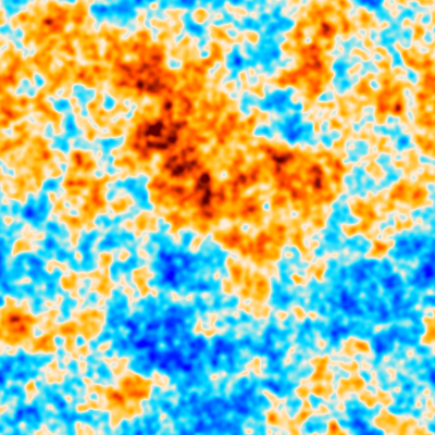
Figure 1: Preview of the model error bias we will discuss in the following sections. Despite the standard expectations that maximum-likelihood mapmaking is optimal and unbiased, the maximum-likelihood solution (right) for a simple toy example is strongly power-deficient on large scales compared to the input signal (left). As we shall see this bias is not unique to maximum-likelihood methods, and can be triggered by several subtle types of model error.

Given this data model, it’s possible to either directly solve for an unbiased map (as in maximum likelihood mapmaking or destriping), or to measure and correct for the bias in a biased estimator (as in filter+bin mapmaking). However, this fails when the model does not actually describe the data, and this turns out to be the norm rather than the exception. Previously this bias has been thought of as mainly a small-scale effect relevant only in regions of the sky with very high contrast, leading to artifacts like thin stripes or bowling around bright sources (Piazzo, 2017; Naess, 2019), or as a tiny correction on intermediate scales (Poutanen et al. (2006) saw a bias of 0.6% peaking at $\ell=800$ for simulations of the Planck space telescope). The goal of this paper is to demonstrate the unintuitive and surprising result that that these effects can lead to $\mathcal{O}(1)$ bias on large scales everywhere in the map. The full scope of these errors appears to be largely unappreciated, and we fear that some published results may suffer from uncorrected bias at low multipoles in total intensity due to these effects. As we shall see, it’s mainly ground-based telescopes that are vulnerable to this bias, which usually manifests as a power deficit at large scales, as illustrated in figure 1.

2 Subpixel errors

a	b

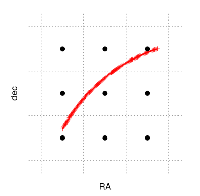
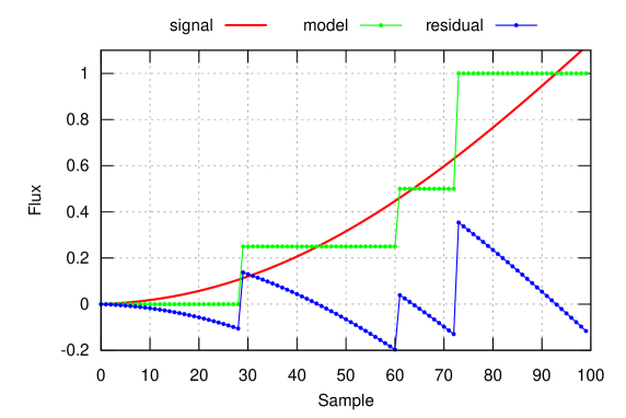
Figure 2: a: Example path (red) of a detector across a few pixels. The area closest to each pixel center (black dots) is shown with dotted lines. In the nearest neighbor model, the value associated with each sample is simply that of the closest pixel, regardless of where inside that pixel it is. b: Example detector signal (red) for the same path. The closest matching model (green) leaves a jagged residual (blue) that has power on all length scales despite the signal itself being very smooth. For comparison, if our model were a constant zero, then the residual would just be the signal itself (red), and hence smooth. If smooth residuals are much cheaper in the likelihood than jagged ones, then a zero model will be preferred to one that hugs the signal as tightly as possible like the green curve.

Subpixel errors may be both the most common and most important class of model errors in CMB mapmaking. For efficiency reasons $P$ is almost always chosen to use simple nearest-neighbor interpolation, where the value of a sample is simply given by the value of the pixel nearest to it. This means that $P$ can be implemented by simply reading off one pixel value per sample, and its transpose $P^{T}$ consists of simply summing the value of the samples that hit each pixel. However, this comes at the cost of there being a discontinuous jump in values as one scans from one pixel to the next, as illustrated in figure 2. Hence, the closest the model can get to a smooth curve is a staircase-like function that hugs it, leaving a residual full of discontinuous jumps (the blue curve in the figure).

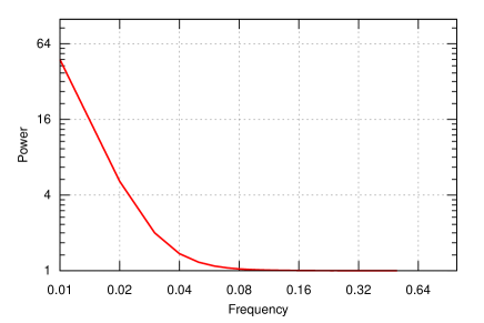
Figure 3: The noise model/inverse weights/inverse filter used in the subpixel bias demonstration in figures 4 and 5. It is a simple Fourier-diagonal 1/f + white noise spectrum typical for ground-based CMB observations. The frequency axis is in dimensionless units in this toy example, but for real telescopes the transition from white noise is typically a few Hz, corresponding to multipoles of hundreds on the sky. The power axis is dimensionless here, but for a real-world case could have units like $\micro$K²/Hz.

Discontinuous residuals are not necessarily problematic. The trouble arises when this is coupled with a likelihood where some modes have much less weight than others. Ground-based CMB telescopes suffer from atmospheric emission that acts as a large source of noise on long timescales. This leads to time-ordered data noise power spectra similar to the one sketched in figure 3, with a white noise floor at short timescales (high frequency) transitioning to a steep rise of several orders of magnitude as one moves to longer timescales (low frequency). In this case long-wavelength modes have orders of magnitude lower weight in the likelihood than short-wavelength modes. Put another way, they are orders of magnitude cheaper to sacrifice when the model can’t fully fit the data.

2.1 1D toy example

To illustrate the interaction between a nearest neighbor pointing matrix’s subpixel errors and a likelihood where large scales have low weight, let us consider a simple 1D case where 100 samples scan uniformly across 10 pixels:

⬇

npix = 10

nsamp = 100

pix = np.arange(nsamp).astype(float)*npix/nsamp

A standard nearest-neighbor pointing matrix for this looks like:

⬇

P = np.zeros((nsamp,npix))

for i, p in enumerate(pix):

P[i,int(np.round(pix[i]))%npix] = 1

We assume a typical Fourier-diagonal “1/f” noise model $N(f)=1+(f/f_{\text{knee}})^{\alpha}$ with $f_{\text{knee}}=0.03$ and $\alpha=-3.5$, and build the inverse noise matrix/filter/baseline-prior $F$ by projecting the inverse noise spectrum $N^{-1}$ into pixel space:

⬇

freq = np.fft.rfftfreq(nsamp)

inv_ps = 1/(1+(np.maximum(freq,freq[1]/2)/0.03)**-3.5)

F = np.zeros((nsamp,nsamp))

I = np.eye(nsamp)

for i in range(nsamp):

F[:,i] = np.fft.irfft(inv_ps*np.fft.rfft(I[i]), n=nsamp)

The signal itself consists of just a long-wavelength sine wave:

⬇

signal = np.sin(2*np.pi*pix/npix)

With this in place, we can now define our map estimators.

2.1.1 Binning

The binned map is simply the mean value of the samples in each pixel, with no weighting:

⬇

map_binned = np.linalg.solve((P.T.dot(P)), P.T.dot(signal))

This is the unweighted least-squares solution for the map. With a nearest neighbor pointing matrix where each sample only affects one pixel $P^{T}P$ is diagonal, making solving for the binned map very fast.

2.1.2 Maximum-likelihood

The maximum-likelihood solution of equation 1 for the sky image $m$ is

$$\hat{m}=(P^{T}N^{-1}P)^{-1}P^{T}N^{-1}d$$ (2)

where $N$ is the covariance matrix of the noise $n$. This is the generalized least-squares solution for the map. Unliked binned mapmaking, the matrix $P^{T}N^{-1}P$ except for the special case of uncorrelated noise. Solving for the maximum-likelihood map can therefore be hundreds of times slower, and requires iterative methods for large maps. In our toy example, $N^{-1}=F$, so the maximum-likelihood map is

⬇

map_ml = np.linalg.solve((P.T.dot(F).dot(P)),P.T.dot(F.dot(signal)))

2.1.3 Filter+bin

As the name suggests, filter+bin consists of filtering the time-ordered data, and then making a binned map. We’ll use $F$ as our filter, so the filter+bin map is

⬇

map_fb = np.linalg.solve(P.T.dot(P), P.T.dot(F).dot(signal))

The filter+bin map is biased by design, so to interpret or debias it one needs to characterize this bias. There are two common approaches to doing this: Observation matrix and simulations.

Observation matrix

The observation matrix approach recognizes that the whole chain of operations observe, filter, map together make up a linear system, and can therefore be represented as a matrix, called the observation matrix (BICEP2 and Keck Array Collaboration, 2016). Building this matrix is heavy, but doable for some surveys. Under the standard assumption that the observation step is given by equation 1, the observation matrix is given by

⬇

obsmat = np.linalg.inv(P.T.dot(P)).dot(P.T.dot(F).dot(P))

and using it, we can define a debiased filter+bin map

⬇

map_fb_deobs = np.linalg.solve(obsmat, map_fb)

Simulations

Alternatively, and more commonly, one can characterize the bias by simulating the observation of a set of random skies, passing them through the filter+bin process, and comparing the properties of the input and output images (e.g. Sayre et al., 2020). The standard way of doing this is by assuming that equation 1 describes the observation process, and that the bias can be described by a transfer function: a simple independent scaling of each Fourier mode. Under these assumptions, we can measure and correct the bias as follows.

⬇

nsim = 1000

sim_ips = np.zeros(npix//2+1)

sim_ops = np.zeros(npix//2+1)

for i in range(nsim):

sim_imap = np.random.standard_normal(npix)

sim_omap = np.linalg.solve(P.T.dot(P), P.T.dot(F).dot(P).dot(sim_imap))

sim_ips += np.abs(np.fft.rfft(sim_imap))**2

sim_ops += np.abs(np.fft.rfft(sim_omap))**2

tf = (sim_ops/sim_ips)**0.5

map_fb_detrans = np.fft.irfft(np.fft.rfft(map_fb)/tf, n=npix)

2.1.4 Destriping

Destriping splits the noise into a correlated and uncorrelated part, and models the correlated noise as a series of slowly changing degrees of freedom to be solved for jointly with the sky image itself (Sutton et al., 2010; Tristram et al., 2011). The data is modeled as

$$d =Pm+Qa+n_{w}$$ (3)

where $n_{w}$ is the white noise with diagonal covariance matrix $N_{w}$, and $Q$ describes how each correlated noise degree of freedom $a$ maps onto the time-ordered data, typically in the form of seconds (ground) to minutes (space) long baselines. Given this, the maximum-likelihood solutions for $a$ and $m$ are

$$Z =I-P(P^{T}N_{w}^{-1}P)^{-1}P^{T}N_{w}^{-1}$$

$$a =(Q^{T}N_{w}^{-1}ZQ+C_{a}^{-1})^{-1}Q^{T}N_{w}^{-1}Zd$$

$$m =(P^{T}N_{w}^{-1}P)^{-1}P^{T}N_{w}^{-1}(d-Qa)$$ (4)

where $C_{a}$ is one’s prior knowledge of the covariance of $a$. Similarly to binned and filter+bin mapmaking, destriping derives its speed from the diagonality of $P^{T}N_{w}^{-1}P$ allowing for instant inversion. On the other hand, the equation for the baseline amplitudes $a$ is not diagonal, and destriping allows a speed/optimality tradeoff in the choice of baseline length and prior. It approaches the maximum likelihood map when the baseline length is a single sample and $C_{a}+N_{w}=N$. We implement this limit below, but explore other choices in section 2.2. In our toy example $N_{w}=I$, so $C_{a}=F^{-1}-I$.

⬇

iCa = np.linalg.inv(np.linalg.inv(F) - I)

Z = I-P.dot(np.linalg.solve(P.T.dot(P), P.T))

a = np.linalg.solve(Z+iCa, Z.dot(signal))

map_ds = np.linalg.solve(P.T.dot(P), P.T.dot(signal - a))

2.1.5 Results

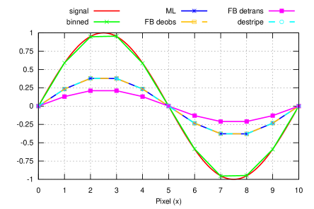
Figure 4: Demonstration of large loss of power in long-wavelength mode caused by the poor subpixel treatment in the standard nearest-neighbor pointing matrix. The vertical axis is dimensionless in this toy example, but could have units like $\micro$K or Jy/sr for a real-world case. Figure 3 shows the noise model/inverse weights/inverse filter used in the various methods. signal: The input signal, a smooth long-wavelength mode, sampled at 10 samples per output pixel. binned: Simple binned map (the unweighted average per pixel). Very suboptimal in the presence of correlated noise, but unbiased. ML: Maximum-likelihood map. 2/3 of the signal amplitude is lost despite the naive expectation of biaslessness for this estimator. FB deobs: Filter+bin map debiased using an observation matrix. Identical to ML. FB detrans: Filter+bin map debiased by deconvolving a transfer function measured from simulations. Even more biased than the others due to ignoring mode coupling. destripe: Destriper in the maximum-likelihood limit (1-sample baselines with optimal baseline prior). Identical to ML.

Figure 4 compares the recovered 1D sky “images” for the different mapmaking methods for this toy example. All methods are expected to have a small loss of power at small scale (called the “pixel window”) due to averaging the signal within each pixel, but this effect is well-known, easy to model, and not our focus here. We deconvolve it using the following function before plotting.

⬇

def dewin(x): return np.fft.irfft(np.fft.rfft(x)/np.sinc(freq),n=len(x)).real

After pixel window deconvolution the binned map (green) closely matches the input signal (red). The same can not be said for the other estimators. Maximum likelihood, filter+bin with observation matrix debiasing and destriping (which are all equivalent in the limit we consider here) are strongly biased, with the signal only being recovered with 1/3 of its real amplitude.

The situation is even worse for filter+bin with simulation-based debiasing, as this suffers from an additional bias due to assuming that the Fourier modes are independent.

2.1.6 Explanation

To see why inaccuracies in modeling the signal at sub-pixel scales can bias the largest scales in the map, let us consider the example in figure 2, where a detector measures a smooth, large-scale signal while moving across a few pixels. With a nearest-neighbor pointing matrix it is impossible to model this smooth signal: the model for each sample is simply that of the closest pixel, regardless of where inside that pixel it is. The model therefore looks like a staircase-like function in the time domain.

Given that we can’t exactly match the signal, what is the best approximation? Let us consider two very different alternatives. Model A: The value in each pixel is the average of the samples that hit it, making the model curve trace the smooth signal as closely as it can. This is the green curve in figure 2, and has the sawtooth-like residual shown with the blue curve. It is probably the model most people would choose if asked to draw one manually. Model B: The value in each pixel is zero, and the residual is simply the signal itself. Model B seems like a terrible fit to the data, but under a reasonable noise model for a ground-based telescope, like the one shown in figure 3, it will actually have a higher likelihood (lower $\chi^{2}=r^{T}N^{-1}r$ where $r$ is the residual) than model A. The reason is that while model B has a much larger residual than model A, model B’s residual is smooth and hence has most of its power at low frequency in the time domain where $N^{-1}$ is very small. Meanwhile, model A’s residual extends to all frequencies due to its jagged nature, including the costly high frequencies. The actual maximum-likelihood solution will be intermediate between these two cases, sacrificing some but not all of the large-scale power in the model to make the residual smoother.

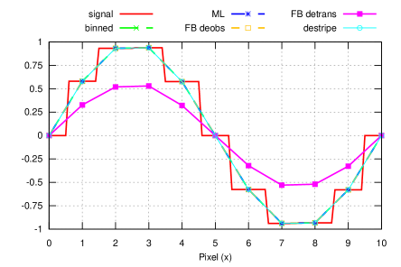
Figure 5: Like figure 4, but with the input signal having the same nearest-neighbor pixelization as the models. In this case all models except FB detrans are unbiased.

To demonstrate that the bias really is caused by subpixel errors, we repeated the simulation with a signal that follows the same nearest-neighbor behavior as the data model, thus eliminating subpixel errors. The result is shown in figure 5. The bias has disappeared in all methods except filter+bin with transfer-function based debiasing, which has an additional source of bias due to its assumption of a Fourier-diagonal filter response.

2.2 2D toy example

The 1D toy example is useful for understanding the origin of the bias, but its unrealistic observing pattern makes it insufficient for exploring optimality/bias tradeoffs in the different methods. We therefore made a larger toy example where a single detector scans at constant speed across a square patch, sampling $N_{\text{scan}}=400$ equi-spaced rows with $N_{\text{scan}}$ equi-spaced samples per row, followed by a column-wise scan the same patch, leading to a total cross-linked data set $N_{\text{samp}}=2N_{\text{scan}}^{2}=3200$ samples long. This equi-spaced grid of samples was chosen to make it easy to simulate a signal directly onto the samples without needing the complication of pixel-to-sample projection. These samples will then be mapped onto a square grid of pixels with a side length of $N_{\text{side}}=100$ using the different mapmaking methods.

For the signal we draw realizations from a CMB-like $1/l^{2}$ power spectrum with a Gaussian beam with standard deviation $\sigma=3$ pixels. Here $l$ is the pixel-space wave-number, which we evaluate in the higher resolution sample space as

⬇

ly = np.fft.fftfreq(N_scan)[:,None] * N_side/N_scan

lx = np.fft.fftfreq(N_scan)[None,:] * N_side/N_scan

l = (ly**2+lx**2)**0.5

With this we can define the signal power spectrum $C_{l}=l^{-2}$ and beam $B_{l}=\exp(-l^{2}\sigma^{2}/2)$, and draw signal realizations as

⬇

signal_map = np.fft.ifft2(np.fft.fft2(np.random.standard_normal((N_scan,N_scan)))*Cl**0.5*Bl).real

signal_tod = np.concatenate([signal_map.reshape(-1), signal_map.T.reshape(-1)])

The last step here takes into account that the simulated scanning pattern covers the field twice, first horizontally and then vertically.

For the noise we use a simple 1/f spectum $N(f)=1+(f/f_{\text{knee}})^{\alpha}$, with f = np.fft.rfftfreq(N_samp) and the knee frequency $f_{\text{knee}}$ corresponding to 1/30th of the side length, $f_{\text{knee}}=0.5\cdot 30/N_{\text{scan}}=0.0375$ (6.7 pixel wavelength), and with an atmosphere-like exponent $\alpha=-3.5$.

The pixel coordinates of each sample are

⬇

pix_pat1 = (np.mgrid[:N_scan,:N_scan]*N_side/N_scan).reshape(2,-1)

pix_pat2 = pix_pat1[::-1]

pix = np.concatenate([pix_pat1,pix_pat2],1)

which we use to build the nearest-neighbor pointing matrix

⬇

iy, ix = np.floor(pix).astype(int)%N_side

P_nn = scipy.sparse.csr_array((np.full(N_samp,1),(np.arange(N_samp),iy*N_side+ix)),shape=(N_samp,N_pix))

	Signal	Noise			Noise	Signal
Input							bin
ML							DS 4
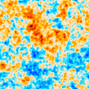
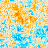
ML w1							DS+ 4
ML w2							DS 64
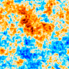
ML w3							DS+ 64
ML lin							DS+ 4 lin

Figure 6: Example signal and noise maps for the different mapmaking methods. The top left map is the input signal, which is directly evaluated at 4x higher resolution than what is used for reconstructing the output maps. All output maps were built from the same data and assume a nearest neighbor pointing matrix, except for the last row where a bilinear pointing matrix was used. The color range is the same for all panels. The binned map (top right) is bias-free but has uselessly high noise. Maximum likelihood (ML) and destriping with short baselengths (with (DS+) and without (DS) baseline amplitude prior, which only matters for the shortest baselines) are all low-noise but biased on large scales. This bias goes away as the noise model is artificially whitened (ML w$X$) or the baseline length is increased (for destriping), but this comes at a cost of increased noise on all scales. Bilinear mapmaking (last row) instead avoids the bias by eliminating most of the model error. It can be difficult to judge how significant the bias and noise levels are from these images. See figures 7 and 8 for easier to interpret comparisons of the signal and noise power spectra respectively.

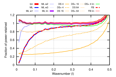
Figure 7: Comparison of the subpixel bias of different mapmaking methods described in section 2.2.1 and discussed in section 2.2.2. Standard maximum-likelihood (thick blue) is strongly biased, as are all but the (very noisy) longest destriping baseline. This bias disappears (ML) or is greatly reduced (DS) when switching to bilinear interpolation in the pointing matrix. See figure 8 for the corresponding noise spectra. The wavenumber $l$ is dimensionless and with a Nyquist frequency of 0.5. we interpret the upturn at $l>0.4$ as aliasing, which is expected and not relevant for the biases we consider here.

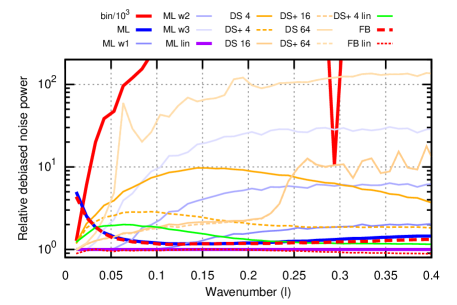
Figure 8: Comparison of the optimality for the methods defined in section 2.2.1, measured as the debiased noise power spectrum (using the bias measurements from figure 7) for each method relative to that of bilinear maximum-likelihood mapmaking. Note the logarithmic vertical axis, and that the binned case was divided by $10^{3}$ to bring it partially inside the plot bounds. The wavenumber $l$ is dimensionless and with a Nyquist frequency of 0.5. It’s clear that simple bias mitigation methods like artificially whitening the noise model or increasing the baseline length are too costly to be practical.

2.2.1 Cases

We will investigate 5 classes of nearest-neighbor maps:

1. bin: Simple binned map, which we expect to be unbiased but very noisy

2. ML: Maximum-likelihood map. Ideally unbiased and optimal, but will deviate from this due to model errors.

3. ML w$X$: Maximum-likelihood maps with a “whitened” noise model, which overestimates the white noise power by a factor $10^{X}$, $X\in\{1,2,3\}$, reducing the overall correlatedness of the noise model. We expect the bias to be proportional to the overall dynamic range of the noise model, so making the noise model whiter should reduce bias. The cost will be suboptimal noise weighting, leading to a noisier map, but it might be worth it.

4. DS $X$: Destriping map with a baseline of $X\in\{4,16,64\}$ samples and no amplitude prior. This is probably the most common type of destriping. The baseline lengths can be compared with the noise knee wavelength of 6.7 pixels $\approx$ 27 samples. This is the wavelength where the correlated and white noise powers are equal.

5. DS+ $X$: Like DS $X$, but uses the correlated part of the maximum-likelihood noise model as an amplitude prior ($C_{a}$ in equation 4).

6. FB: Filter+bin mapmaking where a transfer function is measured using simulations based on the data model, and this is deconvolved when measuring the power spectrum. This is the standard approach for filter+bin mapmaking. In this case only the power spectrum is debiased, not the map, so we don’t show an example map for this case.

Since all the mapmaking methods are linear, the signal and noise can be mapped separately. We make 400 signal-only and noise-only data realizations, and map them using each method, computing the mean signal and noise power spectra.

2.2.2 Results

Example maps are shown in figure 6, while the bias and noise are quantified in figures 7 and 8 respectively. As expected the binned map is unbiased but extremely noisy. The maximum-likelihood map is low-noise, but measurably biased on all scales, with a power deficit of a few percent at the smallest scales which grows to almost 100% on the largest scales. The deficit appears to fall proportionally with the whitening, with ML w1 and w2 being respectively 10x and 100x as close to unbiased. Sadly this comes at the cost of 40% and 350% higher noise power respectively. These numbers may differ for real-world cases, but this still seems like a very expensive bias mitigation method. All but the longest-baseline destriped maps are also strongly biased, with the shortest baseline being considerably worse than ML for almost all scales. Much like we saw with the ML variants, the less biased destriping versions come at a high cost in noise. Finally, the filter+bin map is biased even after simulation-based debiasing due to the simulations not capturing the subpixel behavior of the real data. Both the bias and noise levels are the same as maximum-likelihood in this example.

To test whether the observed biases are truly caused by subpixel errors, we repeat the simulations with only one sample per pixel ($N_{\text{scan}}=N_{\text{side}}$). As expected this results in an unbiased power spectrum for all methods.

2.2.3 Effective mitigation of subpixel errors

There will be no subpixel errors in the limit of infinitely small pixels, so it’s tempting to simply reduce the pixel size to solve the problem. This does work, but since subpixel errors are proportional to $|\nabla s\cdot\vec{\Delta}|$, where $s$ is the true, smooth signal on the sky and $\vec{\Delta}=[\Delta_{x},\Delta_{y}]$ is the pixel shape, the improvement is only first order in the pixel side length. A much more feasible solution is to instead improve the subpixel handling in the pointing matrix. Going from nearest neighbor to bilinear interpolation is enough to practically eliminate subpixel errors without reducing pixel size. We can implement this in the toy example by defining

⬇

pix_left = np.floor(pix).astype(int)

ry, rx = pix-pix_left

iy1,ix1 = pix_left % N_side

iy2,ix2 = (pix_left+1)% N_side

weights = np.concatenate([

(1-ry)*(1-rx), (1-ry)*rx,

ry *(1-rx), ry *rx])

samps = np.tile(np.arange(N_samp),4)

inds = np.concatenate([

iy1*N_side+ix1, iy1*N_side+ix2,

iy2*N_side+ix1, iy2*N_side+ix2])

P_lin = scipy.sparse.csr_array((weights,(samps,inds)),shape=(N_samp,N_pix))

Bilinear mapmaking results in a different pixel window than the standard pixwin_nn = sinc(ly)[:,None]*sinc(lx)[None,:] of nearest neighbor mapmaking. We derive this in appendix A, and the result is pixwin_lin = linwin1d(ly)[:,None]*linwin1d(lx)[None,:], linwin1d(l) = sinc(l)**2/(1/3*(2-cos(2*pi*l))). This is plotted in figure 9.

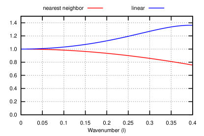
Figure 9: Comparison of the 1D pixel window for nearest neighbor mapmaking (red, $\text{sinc}(l)$) and linear mapmaking (blue). The 2D pixel window is the outer product of the 1D one along each axis. The pixel windows model the response of the Fourier coefficients to binned (unweighted) mapmaking. Square it to get the effect on the power spectrum.

Since each sample in bilinear mapmaking gets contributions from the four closest pixels, the pointing matrix is about four times slower than the standard nearest neighbor version. However, as shown in figures 7 and 8 this cost is worth it, with bilinear maximum-likelihood mapmaking being bias-free and even lower noise than standard ML. The bias is also greatly reduced for destriping, but not eliminated.

Note that bilinear mapmaking (and in general any mapmaking method where each sample affects multiple pixels) breaks the diagonality of $P^{T}P$ which methods like binning, filter+bin and destriping rely on for their speed. While we have implemented bilinear variants of them here in order to investigate the effect on the bias, bilinear filter+bin and bilinear destriping are too slow to be useful in practice. This is in contrast to bilinear maximum-likelihood mapmaking, which only becomes a few times slower.

3 Gain errors

Surprisingly, gain errors can also lead to a scale-dependent power loss. This happens when the noise model correlates observations with inconsistent gain, for example multipe miscalibrated detectors with correlated noise. We will illustrate this using a minimal 1D toy example with two correlated detectors, as well as a more realistic 2D example.

3.1 1D toy example

Consider two miscalibrated detectors scanning across a line of pixels. Both detectors point in the same direction, and take one sample per pixel. We can model this as

$$d =G(Pm+n)=GPm+Gn$$ (actual) (5)

where $d$ is the vector of samples, $m$ is the true signal in the pixels, $n$ is Gaussian noise with covariance $N$, $P$ is the pointing matrix and $G$ is the gain error. Written out in terms of detectors and samples, we can express this as

$$d_{di} =G_{d}P_{d}m_{i}+G_{d}n_{di}$$ (6)

with $d$ and $i$ being the detector and sample index respectively, $P_{d}=[1,1]_{d}=1$ and $G_{d}=[g_{1},g_{2}]_{d}$. This simply expresses that both detectors see the same signal at the same time. Let us assume that the noise covariance is diagonal in Fourier space

$$N_{d_{1}d_{2}ff^{\prime}} =A_{f}C_{fd_{1}d_{2}}\delta_{ff^{\prime}}$$ (7)

$$C_{fd_{1}d_{2}} =\begin{bmatrix}1&\alpha_{f}\\ \alpha_{f}&1\end{bmatrix}$$ (8)

where $f$ and $f^{\prime}$ are frequency indices, and $A_{f}$ is the noise power spectrum. This gives us the inverse noise model

$$N_{d_{1}d_{2}ff^{\prime}}^{-1} =A_{f}^{-1}C_{fd_{1}d_{2}}^{-1}\delta_{ff^{\prime}}$$ (9)

$$C_{fd_{1}d_{2}}^{-1} =(1-\alpha_{f}^{2})^{-1}\begin{bmatrix}1&-\alpha_{f}\\ -\alpha_{f}&1\end{bmatrix}$$ (10)

The maximum-likelihood solution of equation 5 is

$$\hat{m} =(P^{T}GG^{-1}N^{-1}G^{-1}GP)^{-1}P^{T}GG^{-1}N^{-1}G^{-1}d$$

$$=(P^{T}N^{-1}P)^{-1}P^{T}N^{-1}(Pm+n)$$

$$=Pm+n$$ (11)

which has expectation value $\langle\hat{m}\rangle=m$, which is unbiased. However, given that $G$ is supposed to be a gain error, we are presumably not aware of it, and so our data model will instead be

$$d =Pm+Gn$$ (model) (12)

The reason why $G$ is still present in front of $n$ in the model is that the noise properties are almost always measured from the data, so our noise model would automatically absorb $G$. For example, if a detector were to be calibrated too high, it would also appear noisier, and would therefore be downweighted more under inverse variance weigting. Given this model, our maximum-likelihood solution for $m$ is

$$\hat{m} =(P^{T}G^{-1}N^{-1}G^{-1}P)^{-1}P^{T}G^{-1}N^{-1}G^{-1}d$$ (13)

Inserting the actual data behavior from equation 5, we get

$$\langle\hat{m}\rangle =(P^{T}G^{-1}N^{-1}G^{-1}P)^{-1}P^{T}G^{-1}N^{-1}G^{-1}GPm$$

$$=(P^{T}G^{-1}N^{-1}G^{-1}P)^{-1}P^{T}G^{-1}N^{-1}Pm$$ (14)

Since $N$ is diagonal in Fourier space and both $G$ and $P$ are constant in time, the whole equation becomes Fourier-diagonal

$$\langle\hat{m}_{f}\rangle =(P^{T}G^{-1}N_{f}^{-1}G^{-1}P)^{-1}P^{T}G^{-1}N_{f}^{-1}Pm_{f}$$ (15)

Inserting eq. 9, this simplifies to ($A_{f}$ cancels)

$$\langle\hat{m}_{f}\rangle =g_{1}g_{2}\frac{g_{1}+g_{2}}{g_{1}^{2}+g_{2}^{2}}\frac{1-\alpha_{f}}{1-\frac{2g_{1}g_{2}}{g_{1}^{2}+g_{2}^{2}}\alpha_{f}}m_{f}$$ (16)

So the effect of the gain miscalibration is an overall scaling of the result as one would expect, $g_{1}g_{2}(g_{1}+g_{2})/(g_{1}^{2}+g_{2}^{2})$, times a transfer function

$$\text{TF}(f) =\frac{1-\alpha_{f}}{1-\frac{2g_{1}g_{2}}{g_{1}^{2}+g_{2}^{2}}\alpha_{f}}$$ (17)

This reduces to 1 both when the detectors are uncorrelated ($\alpha_{f}=0$) and when there are no relative gain errors ($g_{1}=g_{2}$).

To motivate a frequency-dependent correlation coefficient, let’s consider the common case of atmospheric 1/f-noise plus white instrumental noise. Our detectors are co-pointing, meaning they see the same atmosphere, so this nosie component is 100% correlated between detectors, but we assume their instrumental noise to be uncorrelated.

$$N_{f} =\begin{bmatrix}1&1\\ 1&1\end{bmatrix}(f/f_{\text{knee}})^{-3}+\begin{bmatrix}1&0\\ 0&1\end{bmatrix}=\begin{bmatrix}1&\alpha_{f}\\ \alpha_{f}&1\end{bmatrix}A_{f}$$

$$\alpha_{f} =1-A_{f}^{-1}\quad,\quad A_{f}=1+(f/f_{\text{knee}})^{-3}\quad\Rightarrow$$

$$\text{TF}(f) =\frac{A_{f}^{-1}}{1-\frac{2g_{1}g_{2}}{g_{1}^{2}+g_{2}^{2}}(1-A_{f}^{-1})}$$ (18)

The result is a frequency-dependent correlation coefficient that changes smoothly from 100% corrleated for atmosphere-dominated scales (low frequencies) to 0% correlated for detector-noise dominated scales (high frequencies). The transfer function for this is plotted in figure 10 for the case of a 10% gain error and average weather (tough note that this 1D example does not capture the benefits of crosslinking).

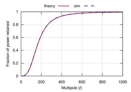
Figure 10: Signal loss for a 1D toy example with noise properties similar to a ground-based CMB telescope average weather (per-detector $\ell_{\text{knee}}=1000$) and a 10% gain error. The solid red curve is based on equation 18. The dashed blue curve is a simulation (gain/gain_model_error_toy_1d_sim.py). Unlike the other examples, the horizontal axis uses multipoles instead of Nyquist units to make it easier to compare to CMB observations.

3.2 2D toy example

We have also demonstrated the effect of gain errors on a somewhat more realistic 2D simulation, where an array of four detectors scans first horizontally and then vertically across a grid of $200\times 200$ pixels, with one sample per pixel and each sample hitting the pixel center to avoid subpixel errors.

The detectors are offset by (0,0), (0,1), (1,0) and (1,1) pixels from the first so that the array instantaneously observes more than just a single pixel, but still only a fraction of the whole image, much like a real detector array would. Each detector has a (constant) gain error drawn independently from a normal distribution with a standard deviation of 0.1, and both the data and noise model reflect this.

The noise model consists of white noise plus a common mode with a $1/\ell$ spectrum with a spectral index of $-3.5$ and $\ell_{\text{knee}}=0.125$ (corresponding to 1/50th of the image side length). This common mode makes the noise model strongly correlated on large scales, like the atmosphere does for real ground-based observations. The bias requires inconsistent observations to be correlated, so the common mode is crucial for this demonstration.

We solve for binned, maximum-likelihood and filter+bin maps using a data model that is unaware of the gain errors (as one would be in reality, or they wouldn’t be gain errors). This is implemented in the program gain_mode_error_2d_toy.py (see section 7).

As expected from the 1D toy example, the gain inconsistency results in a large loss of power on large scales, as shown in figure 11. Filter+bin mapmaking is no less vulnerable to this bias than maximum-likelihood. Figure 12 shows the corresponding relative noise spectra. And as we saw for subpixel errors, attempting to mitigate the bias by artificially reducing the correlations in the noise model is much too costly noise-wise to be a practical mitigation strategy.

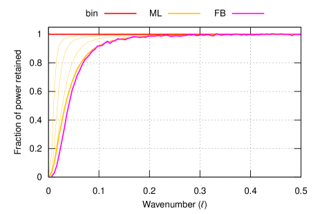
Figure 11: Power loss for a 2D toy example with multiple detectors with inconsistent but constant gain errors. Plain unweighted binning (red) is unbiased, but both maximum-likelihood (blue) and filter+bin (yellow) lose much of the signal at large scales (low wavenumber). The light blue curves are maximum-likelihood with 10/100/1000 times as much white noise in the noise model, reducing the overall correlatedness of the noise. This results in less bias, but also much more noise as shown in figure 12.

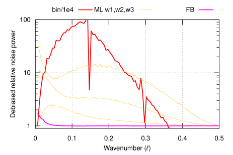
Figure 12: How noisy different mapmaking methods are compared to maximum-likelihood for the 2D gain error toy example. Each graph is the ratio of the transfer-function-deconvolved noise spectrum for binned mapmaking (red), whitened maximum-likelihood (light blue) or filter+bin (yellow) divided by the corresponding spectrum for standard maximum-likelihood. The whitened curves correspond to a noise model with 10/100/1000 times exaggerated white noise floor for the bottom/middle/top light blue curve. Both these and binned mapmaking are too costly to be realistic solutions to the power loss problem. Note the logarithmic y axis and that the binned curve has been divided by $10^{4}$ to fit in the graph.

Detectors with strongly correlated noise on large scales and O(10%) gain error inconsistency are not unrealistic for a ground-based CMB telescope, so it is likely that many ground-based telescopes suffer from this bias to some extent.

3.3 Time-dependent gain errors are much less serious

So far we have only considered cases where detectors disagree on the gain, but gain errors can also be time-dependent. Can these also cause large-scale power loss? As we shall see the answer is “yes, but only in unrealistic circumstances”.

Consider a single detector that makes a series of passes over a line of pixels, such that

$$d_{ix} =g_{ix}m_{x}+g_{ix}n_{ix}\quad\text{(actual)}$$ (19)

where $d_{ix}$ is the measurement in pixel/sample $x$ of pass $i$, $m_{x}$ is the true signal in pixel $x$, $g_{ix}$ is the unmodeled gain and $n_{ix}$ is the noise. We assume that the gain error is ignored in the data model but captured by the noise model:

$$d_{ix} =m_{x}+g_{ix}n_{ix}\quad\text{(model)}$$ (20)

This has maximum-likelihood solution

$$\left(\sum_{i}g_{ix}^{-1}N_{xy}^{-1}g_{iy}^{-1}\right)\hat{m}_{y} =\sum_{i}g_{ix}^{-1}N_{xy}^{-1}(m_{y}+n_{iy})$$ (21)

We further assume

1. Both the noise and gain errors are independent between each pass

2. The inverse gain perturbation $\gamma_{ix}=g_{ix}^{-1}-1$ has stationary covariance $\Gamma$, which is therefore diagonal in Fourier space, with diagonal $\widetilde{\Gamma}$ (its power spectrum).

3. Similarly the covariance is Fourier-diagonal with power spectrum $\widetilde{N}$

Under these assumptions it can be shown (see appendix B) that when the number of passes is much greater than one the Fourier transform of the maximum likelihood solution becomes

$$\hat{\widetilde{m}}_{f} =\frac{\widetilde{N}^{-1}_{f}}{\widetilde{N}^{-1}_{f}+S^{-2}(\widetilde{\Gamma}\ast\widetilde{N}^{-1})_{f}}\widetilde{m}_{f}$$ (22)

where $\ast$ is the convolution operator and $S$ is the number of pixels, and we’ve assumed the standard discrete Fourier transform normalization. We see that in the limit of uncorrelated gain errors, $\widetilde{\Gamma}_{f}=\text{const}$, the bias becomes $1/(1+\text{const}\cdot\widetilde{N})$. For atmospheric noise this gives a strong suppression of the signal on large scales, just like we saw for detector errors. On the other limit where the gain error changes slowly and is approximately constant over a noise correlation length, we have $\widetilde{\Gamma}\approx\text{const}\cdot\delta\Rightarrow\widetilde{\Gamma}\ast\widetilde{N}^{-1}\approx\text{const}\cdot\widetilde{N}^{-1}$, and so the bias just becomes a constant scaling. So to get scale-dependent power loss, the gain error needs to vary on time-scales over which the noise is strongly correlated.

However, all of this rests on the assumption that the gain errors are captured by the noise model. For the previous case of constant per-detector gain errors this is realistic - after all detectors typically don’t all have the same noise level, so they need to be weighted differently, and the noise model ends up absorbing the gain error when being measured from the data itself. The situation is different from time-dependent gains. As we saw above, the noise model must be modulated by gain errors that change quickly relative to the atmosphere if we are to get scale-dependent bias, and for a typical ground-based CMB telescope this works out to be $\sim$ second time-scales. It is very uncommon to build noise models that track the noise properties with a time resolution this high.

In contrast to detector-dependent gain errors, we therefore do not expect time-dependent gain errors to be a significant source for large-scale power loss.

4 Easily missed in simulations

What makes model error bias especially insidious is that it is completely invisible to any simulation that does not explicitly include that particular type of model error. For example, a simulation where the CMB is read off from a simulated map using the same pointing matrix as is used in the mapmaking itself would be blind to subpixel errors. And simulations that don’t inject gain errors into both the data and noise model will be blind to power loss from gain errors. Given the many possible ways the real data might deviate from one’s model of it, it is hard to be sure that one has included all the relevant types of model error in the simulations. It is therefore very easy to trick oneself into believing that one has an unbiased analysis pipeline while there are in fact $\mathcal{O}(1)$ biases remaining.

5 Detection strategies

The unintuitive large-scale effects of model errors originate from the interaction between model errors and non-local weighting/filtering. A noise model (or filter) with a large dynamic range, such as one capturing the huge ratio between the long-wavelength and short-wavelength noise power typical for ground-based CMB telescopes, is therefore much more vulnerable to large-scale power loss than one appropriate for space-based telescopes which have almost flat noise power spectra. This suggests the following tests for large-scale model error bias:

1. Compare power spectra with those from a space-based telescope. This is reliable but comes at the cost of being able to make an independent measurement.

2. Split the data into subsets with different ratios of correlated noise to white noise and check their consistency. This could for example be a split by the level of precipitable water-vapor (PWV) in the atmosphere. High-PWV-data would be expected to have a higher dynamic range and therefore be more vulnerable.

3. Map the same data both using the standard noise model/filter and a less optimal one an artificially reduced lower dynamic range, e.g. one that underestimates the amount of correlated noise or ignores correlations between detectors. The latter should result in less a biased but noisier map, as we saw in figures 7 and 8. If the maps are consistent, then large-scale model error bias is probably not an issue. Alternatively, one can check for consistency when varying the pixel size. We haven’t tested the effectiveness of this method, but model error bias should be proportional to the pixel size with nearest neighbor mapmaking.

6 Who is at risk?

While model error bias can be expected to always be present at a low level, it only becomes important when dealing with very large amounts of correlated noise (e.g. much more noise correlations on some scales than others, see equation 18). Therefore, the telescopes at risk are those that fulfill the following criteria.

1. Observe from the ground.

2. Care about total intensity, since the atmosphere is mostly unpolarized.

3. Observe at frequencies with high water vapor emission, since water vapor is the main source of clumpiness in the atmospheric emission. At CMB-relevant frequencies, the lower the frequency the safer. Frequencies $<60$ GHz should be relatively safe while $>200$ GHz are particularly vulnerable.

4. Have sensitive detectors, since lower white noise means a larger ratio between this noise and the correlated noise from the atmosphere.

5. Have a large number of detectors with a low angular separation on the sky, since this increases their correlatedness.

There aren’t that many telescopes that fulfill these criteria, as ground-based telescopes have focused mostly on polarization or lower frequencies. After reviewing LAMBDA’s list of CMB experiments we found four $>60$ GHz ground-based CMB telescope projects started after year 2000 with published TT spectra for $\ell<2000$: ACBAR, ACT, BICEP and SPT. Of these, ACBAR, ACT (Choi et al., 2020) and SPT-3G (Balkenhol et al., 2022) cut their low-$\ell$ data, indicating problems recovering these scales. Meanwhile BICEP (BICEP1 Collaboration, 2013; BICEP2 and Keck Array Collaboration, 2018) and SPTpol (Henning et al., 2018) publish TT spectra down to $\ell<100$ with no signs of problems. The only case where we could see clear evidence for large-scale power-loss is in the multipoles just above the multipole cutoff in ACT, as seen in figure 13 (reproduced from Choi et al. (2020)).

Figure 13: Large-scale power loss in ACT DR4. The ACT TT power spectrum (blue) and the ACT-Planck cross-spectrum (orange) are both low at $\ell\lesssim 800$ compared to the Planck power spectrum (green) in the two ACT patches shown. This is especially clear in the third panel, which shows the difference between ACT and the ACT-Planck cross. Reproduced from Choi et al. (2020).

So to summarize, why hasn’t this been noticed before? Ground-based CMB surveys have mostly focused on polarization, where this effect is orders of magnitude smaller. Those that do publish total intensity power spectra have only reached the high enough sensitivity and detector counts for it to become noticable in the last decade. Given how frequently ground-based CMB surveys cut $\ell\lesssim 500-1000$ it is tempting to speculate that model error bias may have caused null tests to fail at low $\ell$ without being identified as the culprit.

7 Source code

The source code and data files behind these examples is available at https://github.com/amaurea/model_error2. The 1D and 2D subpixel simulations are available in subpix/model_error_toy.py and subpix/model_error_toy.py respectively, while the gain error example is in gain/gain_model_error_toy_2d.py.

8 Conclusion

1. All current CMB mapmaking methods are vulnerable to model error bias, including maximum-likelihood mapmaking, destriping and filter+bin mapmaking.

2. Subpixel errors and gain errors are common examples of model errors, with subpixel errors being almost universal. Subpixel bias is caused by the likelihood disfavoring the sharp edges implied by the pixelization, causing it to discard low-S/N signal. Gain errors enter into inverse variance weighting squared, leading to a noise bias term that dominates strongly downweighted/filtered scales. Other types of model error can also be important.

3. Model error bias can manifest in unintuitive ways, with a common symptom being a large ($\mathcal{O}(1)$) loss of long-wavelength power in the maps.

4. The size of the bias is proportional to the dynamic range of the filter/noise model. Hence it is important for ground-based measurements of the unpolarized CMB due to the presence of large-scale atmospheric noise there, but is much less important for polarization measurements or space-based telescopes.

5. Simulations are blind to these biases unless specifically designed to target them. There is a large risk of ending up thinking one has an unbiased pipeline despite there being large bias in the actual CMB maps.

6. An effective way of testing for this bias is to also map the data using a (much) lower dynamic range noise model/filter and checking if this leads to consistent power spectra.

While it’s unclear how large a role model-error bias has played in ground-based CMB results published so far, it will be an increasingly important effect as sensitivity increases. We hope upcoming projects like Simons Observatory and CMB-S4 will be on the lookout for large-scale power loss in total intensity, and to be aware that simulations alone cannot prove that their analysis pipeline is bias free.

Appendix A Linear pixel window

Let us start by considering the 1D case. Given a set of pixels $\{i\}$ with values $\{v_{i}\}$ we define the linear interpolation value $d$ at some pixel coordinate $i+x$ where $x\in[0,1)$ as

$$d=(1-x)v_{i}+xv_{i+1}$$ (23)

This is illustrated in figure 14.

Figure 14: Definition of the quantities involved in linear interpolation. Given values $\{v_{i}\}$ sampled at locations $\{i\}$, we define the linear interpolation value $d$ at some location $i+x$ where $x\in[0,1)$ as $d=(1-x)v_{i}+xv_{i+1}$.

We can generalize this to a set of samples $d_{a}$ with

$$d_{a} =(1-x_{a})v_{a}^{\text{left}}+x_{a}v_{a}^{\text{right}}$$ (24)

where $v_{a}^{\text{left}}$ and $v_{a}^{\text{right}}$ are the values of the pixel to the left and right of where sample $a$ points, and $x_{a}$ is its subpixel position. This linear system can be written as the following matrix equation

$$d =Pv$$ (25)

$P$’s form will depend on the exact scanning pattern, but the final pixel window should only depend on each pixel being hit equally much at all subpixel locations. For simplicity, we will assume a simple scanning pattern that scans a single time across a row of pixels from left to right, with a constant scanning speed and infinite sample rate. This results in the pointing matrix $P$ taking the form shown in figure 15.

Figure 15: Structure of a linear-interpolation pointing matrix $P$ and its transpose $P^{T}$ for the case of a set of samples making a single scan across a row of pixels in 1D, assuming wrapping boundary conditions. $x\in[0,1)$ is the subpixel coordinate of each sample.

Given the set of samples $d$, the least squares estimator for the pixel values $v$ under uniform weighting is

$$\hat{v} =(P^{T}P)^{-1}P^{T}d$$ (26)

The denominator $P^{T}P$ consists of two types of non-zero cases:

$$(P^{T}P)_{00} =\begin{bmatrix}\cdots&1-x&\cdots\end{bmatrix}\begin{bmatrix}\vdots\\ 1-x\\ \vdots\end{bmatrix}+\begin{bmatrix}\cdots&x&\cdots\end{bmatrix}\begin{bmatrix}\vdots\\ x\\ \vdots\end{bmatrix}=S\int_{0}^{1}(1-x)^{2}dx+S\int_{0}^{1}x^{2}dx=\frac{2}{3}S$$ (27)

$$(P^{T}P)_{01} =\begin{bmatrix}\cdots&1-x&\cdots\end{bmatrix}\begin{bmatrix}\vdots\\ x\\ \vdots\end{bmatrix}=S\int_{0}^{1}(1-x)xdx=\frac{1}{6}S$$ (28)

Here $S$ is the number of samples per pixel, and appears due to the summing implied by $P^{T}$. $S\rightarrow\infty$ in the integral limit we used here, but it will end up cancelling. With this, we end up with the denominator taking the Toeplitz form

$$P^{T}P =\frac{1}{6}N\begin{bmatrix}4&1&&&&&1\\ 1&4&1&&&&\\ &1&4&1&&&\\ &&&\ddots&&&\\ &&&&1&4&1\\ 1&&&&&1&4\end{bmatrix}$$ (29)

Toeplitz matrices are diagonal in Fourier space, so $(P^{T}P)^{-1}$ becomes a simple element-wise division there. The Fourier-diagonal is given by the Fourier transform of the first row of the Toeplitz matrix. Defining $A=P^{T}P$, it’s Fourier diagonal as $\tilde{a}$ is given by

$$\tilde{a}(k) =\frac{1}{N}\sum_{j=0}^{N-1}e^{\frac{-2\pi ikj}{N}}A_{j0}=\frac{S}{N}\frac{1}{6}\Big{(}4+e^{\frac{2\pi ik}{N}}+e^{\frac{-2\pi ik}{N}}\Big{)}=\frac{S}{N}\frac{1}{3}\Big{(}2+\cos\frac{2\pi k}{N}\Big{)}$$ (30)

where $N$ is the number of pixels, $i$ is the imaginary unit, $k$ is the zero-based index into $\tilde{a}$ and $j$is the zero-based row index of $A$.

Turning to the numerator $b=P^{T}d$, we recognize that it is simply the convolution of $d$ with the triangle function $T(x)=(1-|x|)S,x\in[-1,1]$, evaluated at each pixel center. Using the convolution theorem, we can therefore directly write down

$$\tilde{b}(k) =\tilde{T}(k)\cdot\tilde{d}(k)$$ (31)

We’re left with computing the Fourier-space representation of the triangle function $T$.

$$\tilde{T}(k) =\frac{S}{N}\int_{-1}^{1}e^{\frac{-2\pi ikx}{N}}(1-|x|)dx$$

$$=\frac{S}{N}\left[\int_{-1}^{1}e^{\frac{-2\pi ikx}{N}}dx-\int_{0}^{1}e^{\frac{-2\pi ikx}{N}}xdx-\int_{-1}^{0}e^{\frac{-2\pi kx}{N}}(-x)dx\right]$$

$$=\frac{S}{N}\left[2\,\text{sinc}\frac{2k}{N}-2\,\text{sinc}\frac{2k}{N}+2\Big{(}\frac{2\pi k}{N}\Big{)}^{2}\Big{(}1-\cos\frac{2\pi k}{N}\Big{)}\right]$$

$$=\frac{S}{N}\Big{(}\,\text{sinc}\frac{k}{N}\Big{)}^{2}$$ (32)

Combining the numerator and denominator we have

$$\hat{\tilde{v}} =\frac{\tilde{b}(k)}{\tilde{a}(k)}\tilde{d}(k)=\frac{\big{(}\,\text{sinc}\frac{k}{N}\big{)}^{2}}{\frac{1}{3}\big{(}2+\cos\frac{2\pi k}{N}\big{)}}\tilde{d}(k)=W_{\text{lin}}(k/N)\tilde{d}(k)$$ (33)

where the linear interpolation pixel window $W_{\text{lin}}(f)$ is defined as

$$W_{\text{lin}}(f) =\frac{\,\text{sinc}(f)^{2}}{\frac{1}{3}\big{(}2+\cos(2\pi f)\big{)}}$$ (34)

This pixel window is compared to the standard nearest neighbor pixel window $W_{\text{nn}}=\,\text{sinc}(f)$ in figure 16. Their behavior is quite different. While $W_{\text{nn}}$ falls monotonically to around 0.6 at the Nyquiest frequency, $W_{\text{lin}}$ rises to about 1.4 at $f=0.4$, and only then starts falling.

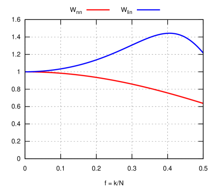
Figure 16: Comparison the 1D pixel windows for nearest neighbor mapmaking ($W_{\text{nn}}$) and linear mapmaking ($W_{\text{nn}}$), plotted up to the Nyquist frequency, which is $\frac{1}{2}$ in these units.

The natural generalization of linear interpolation to two dimensions is bilinear interpolation, which is the composition of a horizontal and vertical one-dimensional interpolation. Because this operation is separable, so is the resulting pixel window. Hence

$$W_{\text{lin}}^{\text{2D}}(f_{y},f_{x}) =W_{\text{lin}}(f_{y})W_{\text{lin}}(f_{x})$$ (35)

Appendix B Time-dependent gain errors

Continuing from section 3.3, we had

$$\underbrace{\left(\sum_{i}g_{ix}^{-1}N_{xy}^{-1}g_{iy}^{-1}\right)}_{A_{xy}}\hat{m}_{y} =\underbrace{\sum_{i}g_{ix}^{-1}N_{xy}^{-1}(m_{y}+n_{iy})}_{b_{x}}$$ (36)

Expanding $g_{ix}^{-1}=1+\gamma_{ix}$ and assuming the detector makes $M$ passes over the pixels, we get

$$A_{xy} =\sum_{i}^{M}(1+\gamma_{ix})N_{xy}^{-1}(1+\gamma_{iy})$$

$$=M\Big{(}N_{xy}^{-1}+\underbrace{\frac{1}{M}\sum_{i}^{M}\gamma_{ix}N_{xy}^{-1}}_{\text{odd}}+\underbrace{\frac{1}{M}\sum_{i}^{M}N_{xy}^{-1}\gamma_{iy}}_{\text{odd}}+\underbrace{\frac{1}{M}\sum_{i}^{M}\gamma_{ix}N_{xy}^{-1}\gamma_{iy}}_{\psi_{xy}}\Big{)}$$ (37)

In the limit $M\rightarrow\infty$ the odd powers of the random variable $\gamma$ disappear, so we are left with computing $\psi$. Since both $N$ and $\Gamma$ are diagonal in Fourier space, it makes sense to express $\psi$ in Fourier space. Denoting Fourier-space quantities with a tilde, and defining the Fourier transform operators

$$F_{kx} =\exp(-2\pi\sqrt{-1}kx/S) F_{xk}^{-1} =\frac{1}{N}\exp(2\pi\sqrt{-1}kx/S)$$ (38)

where $S$ is the number of pixels, we get

$$\widetilde{\psi}_{jk} =\frac{1}{M}\sum_{i}^{M}\sum_{xy}F_{jx}(F^{-1}\widetilde{\gamma})_{x}(F^{-1}\widetilde{N}F^{-1{\dagger}})^{-1}_{xy}(F^{-1}\widetilde{\gamma})_{y}^{\dagger}F_{yk}^{\dagger}$$

$$=\frac{1}{M}\sum_{i}^{M}\sum_{xy}F_{jx}(F^{-1}\widetilde{\gamma})_{x}(F^{\dagger}\widetilde{N}^{-1}F)_{xy}(F^{-1}\widetilde{\gamma})_{y}^{\dagger}F_{yk}^{\dagger}$$

$$=\frac{1}{M}\sum_{i}^{M}\sum_{xy\alpha\beta\gamma}\frac{1}{N^{2}}\exp\Big{(}\frac{2\pi\sqrt{-1}}{S}(\underbrace{-jx+\alpha x+\beta x}_{N\delta_{\beta,j-\alpha}}\underbrace{-\beta y-\gamma y+ky}_{N\delta_{\gamma,k-\beta}})\Big{)}\widetilde{\gamma}_{\alpha}\widetilde{N}_{\beta}^{-1}\widetilde{\gamma}_{\gamma}^{\dagger}\Big{)}$$

$$=\sum_{\alpha}\underbrace{\Big{(}\frac{1}{M}\sum_{i}^{M}\widetilde{\gamma}_{\alpha}\widetilde{\gamma}_{k-j+\alpha}\Big{)}}_{\widetilde{\Gamma}_{\alpha,\alpha+k-j}=\widetilde{\Gamma}_{\alpha}\delta_{k,j}}\widetilde{N}_{j-\alpha}^{-1}$$

$$=\sum_{\alpha}\widetilde{\Gamma}_{\alpha}\widetilde{N}_{j-\alpha}^{-1}\delta_{jk}$$

$$=\Big{(}\widetilde{\Gamma}\ast\widetilde{N}^{-1}\Big{)}_{j}\delta_{jk}$$ (39)

So $\psi$ is Fourier diagonal just like $\Gamma$ and $N^{-1}$, and its diagonal is the convolution of their diagonals. With this we can complete the expression for $A$.

$$\widetilde{A} =FAF^{\dagger}=F\Big{(}(F^{-1}\widetilde{N}F^{-1{\dagger}})^{-1}+F^{-1}\widetilde{\psi}F^{-1{\dagger}}\Big{)}F^{\dagger}=MS^{2}\Big{(}\widetilde{N}^{-1}+S^{-2}\widetilde{\Gamma}\ast\widetilde{N}^{-1}\Big{)}$$ (40)

Moving on to the right-hand-side of the equation for $\hat{m}$, we have

$$b_{x} =\sum_{i}^{M}(1+\gamma_{ix})N_{xy}^{-1}(m_{y}+n_{iy})$$

$$=M\Big{(}N_{xy}^{-1}m_{y}+\underbrace{\frac{1}{M}\sum_{i}^{M}\gamma_{ix}N_{xy}^{-1}n_{iy}}_{\text{odd}}+\underbrace{\frac{1}{M}\sum_{i}^{M}\gamma_{ix}N_{xy}^{-1}m_{y}}_{\text{odd}}+\underbrace{\frac{1}{M}\sum_{i}^{M}\gamma_{ix}N_{xy}^{-1}n_{iy}}_{\text{$\gamma$ and $n$ independent}}\Big{)}$$ (41)

All but the first term fall out if we assume that the fluctuations in $\gamma$ and $n$ are independent. Going to Fourier space, we are left with

$$\widetilde{b} =Fb=MF\Big{(}F^{-1}\widetilde{N}F^{-1{\dagger}}\Big{)}^{-1}F^{-1}\widetilde{m}=M\underbrace{FF^{\dagger}}_{S}\widetilde{N}^{-1}\underbrace{FF^{-1}}_{I}\widetilde{m}=MS\widetilde{N}^{-1}\widetilde{m}$$ (42)

With this the full Fourier-space equation for $\hat{\widetilde{m}}$ becomes:

$$A\hat{m} =b\Leftrightarrow F^{-1}\widetilde{A}\underbrace{F^{-1{\dagger}}F^{-1}}_{S^{-1}}\hat{\widetilde{m}}=F^{-1}\widetilde{b}\Leftrightarrow\hat{\widetilde{m}}=\frac{\widetilde{N}^{-1}}{\widetilde{N}^{-1}+S^{-2}\widetilde{\Gamma}\ast\widetilde{N}^{-1}}\widetilde{m}$$

The factor $S^{-2}$ is an artifact of the Fourier normalization used, and would differ for other Fourier unit choices.

References

- Aiola et al. (2020) Aiola, S., et al. 2020, arXiv:2007.07288, J. Cosmology Astropart. Phys, 2020, 047, The Atacama Cosmology Telescope: DR4 maps and cosmological parameters
- Balkenhol et al. (2022) Balkenhol, L., et al. 2022, arXiv:2212.05642, arXiv e-prints, arXiv:2212.05642, A Measurement of the CMB Temperature Power Spectrum and Constraints on Cosmology from the SPT-3G 2018 TT/TE/EE Data Set
- BICEP1 Collaboration (2013) BICEP1 Collaboration. 2013, arXiv:1310.1422, Degree-Scale CMB Polarization Measurements from Three Years of BICEP1 Data
- BICEP2 and Keck Array Collaboration (2016) BICEP2 and Keck Array Collaboration. 2016, arXiv:1603.05976, ApJ, 825, 66, BICEP2/Keck Array. VII. Matrix Based E/B Separation Applied to Bicep2 and the Keck Array
- BICEP2 and Keck Array Collaboration (2018) —. 2018, arXiv:1810.05216, Phys. Rev. Lett., 121, 221301, Constraints on Primordial Gravitational Waves Using Planck, WMAP, and New BICEP2/Keck Observations through the 2015 Season
- BICEP2 Collaboration (2014) BICEP2 Collaboration. 2014, arXiv:1403.3985, BICEP2 I: Detection Of B-mode Polarization at Degree Angular Scales
- Choi et al. (2020) Choi, S. K., et al. 2020, arXiv:2007.07289, J. Cosmology Astropart. Phys, 2020, 045, The Atacama Cosmology Telescope: a measurement of the Cosmic Microwave Background power spectra at 98 and 150 GHz
- Dutcher et al. (2021) Dutcher, D., et al. 2021, arXiv:2101.01684, Phys. Rev. D, 104, 022003, Measurements of the E -mode polarization and temperature-E -mode correlation of the CMB from SPT-3G 2018 data
- Henning et al. (2018) Henning, J. W., et al. 2018, arXiv:1707.09353, ApJ, 852, 97, Measurements of the Temperature and E-mode Polarization of the CMB from 500 Square Degrees of SPTpol Data
- Keihänen et al. (2010) Keihänen, E., Keskitalo, R., Kurki-Suonio, H., Poutanen, T., & Sirviö, A. S. 2010, arXiv:0907.0367, A&A, 510, A57, Making cosmic microwave background temperature and polarization maps with MADAM
- Keihänen & Reinecke (2012) Keihänen, E. & Reinecke, M. 2012, arXiv:1208.1399, A&A, 548, A110, ArtDeco: a beam-deconvolution code for absolute cosmic microwave background measurements
- Naess (2019) Naess, S. K. 2019, JCAP, 2019, 060–060, How to avoid X’es around point sources in maximum likelihood CMB maps, http://dx.doi.org/10.1088/1475-7516/2019/12/060
- Piazzo (2017) Piazzo, L. 2017, ITIP, 26, 5232, Least Squares Image Estimation for Large Data in the Presence of Noise and Irregular Sampling
- Planck Collaboration (2020) Planck Collaboration. 2020, arXiv:1807.06207, A&A, 641, A3, Planck 2018 results. III. High Frequency Instrument data processing and frequency maps
- Poutanen et al. (2006) Poutanen, T., et al. 2006, astro-ph/0501504, A&A, 449, 1311, Comparison of map-making algorithms for CMB experiments
- Ruud et al. (2015) Ruud, T. M., et al. 2015, arXiv:1508.02778, ApJ, 811, 89, The Q/U Imaging Experiment: Polarization Measurements of the Galactic Plane at 43 and 95 GHz
- Sayre et al. (2020) Sayre, J. T., et al. 2020, arXiv:1910.05748, Phys. Rev. D, 101, 122003, Measurements of B -mode polarization of the cosmic microwave background from 500 square degrees of SPTpol data
- Schaffer et al. (2011) Schaffer, K. K., et al. 2011, arXiv:1111.7245, ApJ, 743, 90, The First Public Release of South Pole Telescope Data: Maps of a 95 deg2 Field from 2008 Observations
- Sutton et al. (2010) Sutton, D., et al. 2010, arXiv:0912.2738, MNRAS, 407, 1387, Fast and precise map-making for massively multi-detector CMB experiments
- Tegmark (1997) Tegmark, M. 1997, AJ, 480, L87–L90, How to Make Maps from Cosmic Microwave Background Data without Losing Information, http://dx.doi.org/10.1086/310631
- Tristram et al. (2011) Tristram, M., Filliard, C., Perdereau, O., Plaszczynski, S., Stompor, R., & Touze, F. 2011, arXiv:1103.2281, A&A, 534, A88, Iterative destriping and photometric calibration for Planck-HFI, polarized, multi-detector map-making