Integrable crosscaps in classical sigma models

Abstract

We study the integrable boundaries and crosscaps of classical sigma models. We show that there exists a classical analog of the integrability condition and KT-relation of the boundary and crosscap states of quantum spin chains. We also classify the integrable crosscaps for various sigma models including examples which are relevant in the AdS/CFT correspondence at strong coupling.

1 Introduction

In recent years, intensive research has been done in the defect versions of AdS/CFT duality. The probe brane defects in the string theory side were introduced in Karch:2001cw and in the gauge theory side they correspond to defect conformal field theories (dCFTs) DeWolfe:2001pq . For theories with domain wall defects, the one-point functions at weak coupling can be obtained from an overlap between a boundary state (corresponding to the defect) and the Bethe states (corresponding to the single trace operators) of a spin chain (describing the scalar sector of the CFT) deLeeuw:2015hxa ; Buhl-Mortensen:2015gfd ; Kristjansen:2021abc . Similar overlaps appear also for the three-point functions which contain one single trace and two determinant type operators Jiang:2019xdz ; Jiang:2019zig ; Yang:2021hrl .

It was possible to write these overlaps in closed forms deLeeuw:2016umh ; DeLeeuw:2018cal ; DeLeeuw:2019ohp ; Gombor:2022aqj . These closed forms were validated only by numerical checks. The reason of the existence such exact overlaps is the underlying integrability of the boundary states. The definition of the integrability for boundary states of spin chains was developed in Piroli:2017sei (based on Ghoshal:1993tm ). We call a boundary state integrable if it preserves the half of the conserved charges of the spin chain. This condition can be written in a compact form

$$\langle B|\mathcal{T}(u)=\langle B|\mathcal{T}^{\beta}(-u),$$ (1)

where $\langle B|$ is the boundary state and $\mathcal{T}(u),\mathcal{T}^{\beta}(u)$ are transfer matrices of the spin chain which are connected by a $\mathbb{Z}_{2}$ automorphism $\beta$ of the underlying symmetry algebra. In Gombor:2021hmj a systematic algebraic method was introduced which proves the previously proposed form of the exact overlaps for a wide class of boundary states. The heart of this derivation is the so-called $KT$-relation

$$K_{0}(u)\langle B|T_{0}(u)=\langle B|T_{0}^{\beta}(-u)K_{0}(u),$$ (2)

where $T(u),T^{\beta}(u)$ are the monodromy matrices and $K(u)$ is the $K$-matrix which acts only on the auxiliary space.

Recently, an other type of states called crosscap states Caetano:2021dbh was introduced for spin chains which are the analogous versions of the crosscap states of 2d CFT Ishibashi:1988kg . The difference between the boundary and the crosscap states are the following. While the boundary states identify the neighboring sites of the spin chain, the crosscap identifies the antipodal sites. In Gombor:2022deb the $KT$-relation was generalized for crosscap states and it was used to classify the crosscap states for all $\mathfrak{gl}(N)$ symmetric spin chains. The previously proposed formula of Caetano:2021dbh for overlaps was also proved for a wide class of crosscap states based on the $KT$-relation. In Caetano:2022mus it was argued that integrable crosscap states are appeared in the one-point functions of the $\mathcal{N}=4$ SYM on the $\mathbb{R}\mathrm{P}^{4}$ spacetime.

As we already mentioned, at strong coupling the defect corresponds to a probe D-brane which can be describe as boundary conditions of the string sigma models. For certain boundary conditions the integrability has been already shown Dekel:2011ja ; Linardopoulos:2021rfq ; Linardopoulos:2022wol . During these derivations the boundaries were putted on space therefore it was showed that infinity many conserved charges exist on the worldsheet of the open strings which are attached on the D-brane. However, in the holographic description of the one-point function we have a closed string (corresponding to the operator) which is annihilated on the D-brane. In this setup the boundary is in time, and intuitively, the integrability means that the boundary condition preserves the half of the worldsheet conserved charges of the closed strings. It is clear that it would be a classical analog of the quantum integrability condition (1).

The goal of this paper is twofold. Firstly, we want to show that classical analogs of the integrability conditions (1) and $KT$-relations (2) exist for classical sigma models with boundaries in time. We also show that these relations are automatically satisfied for the classical reflection matrices of Dekel:2011ja ; Linardopoulos:2021rfq ; Linardopoulos:2022wol . We also generalize the integrability condition and $KT$-relations for the crosscaps of classical sigma models. The second goal is to classify the integrable crosscaps of the sigma models which appear in the AdS/CFT at strong coupling. This paper is not intended to provide a complete holographic description, we will not go beyond the classic sigma model. However, this classification for the sigma models can be a good starting point for more comprehensive future investigations.

The organization of the paper is as follows. In section 2 we give the definition of the crosscaps of sigma models. In section 3 we review the Lax description (Lax-connection, transfer matrix etc.) of the sigma models. In section 4 we derive the integrability condition and $KT$-relation when the boundaries are in time. In section 5 we generalize the integrability condition for crosscaps and classify them for the sigma models with target spaces $SU(N)$, $S^{N-1}$, $AdS_{N-1}$ and $\mathbb{C}\mathrm{P}^{N-1}$. In section 6 we classify the integrable crosscaps of the sigma models which appear in the $AdS_{5}/CFT_{4}$ and $AdS_{4}/CFT_{3}$ dualities at strong coupling.

2 Crosscaps of sigma models

In this section we define the crosscaps for 2d sigma models. Let $\mathcal{M}$ be a semi-Riemann manifold (target space) with local coordinates $X^{I}$ where $I=1,\dots,\dim\mathcal{M}$ and metric $G_{IJ}(X)$. We also define a 2d manifold (worldsheet) with local coordinates $\sigma^{\mu}=\left(\sigma^{0},\sigma^{1}\right)=\left(\tau,\sigma\right)$ and the worldsheet metric $\eta$. The fields in the 2d sigma model are maps between the worldsheet and the target space: $X:\Sigma\to\mathcal{M}$. The dynamics are given by the action

$$S[X]=\int_{\Sigma}d\tau d\sigma G_{IJ}(X)\partial_{\mu}X^{I}\partial^{\mu}X^{J}.$$ (3)

Let $\alpha$ be a $\mathbb{Z}_{2}$ isometry of $\mathcal{M}$ which acts on the fields as $\alpha:X\to X^{\alpha}$. It is clear that if we have a solution $X^{I}(\tau,\sigma)$ of the equations of motion then the transformed fields $X^{\alpha,I}(\tau,\sigma)$ also satisfy them.

At first let us consider an infinite cylinder as worksheet: $\Sigma=\mathbb{R}\times S^{1}$. We choose the local coordinates as $\tau\in\mathbb{R}$ and $\sigma\in\left[0,L\right)$ with the identification $\sigma+L\equiv\sigma$. We define the crosscap by a restriction of the allowed configurations of the fields. We allow only the configurations which are invariant under the following $\mathbb{Z}_{2}$ transformation

$$X(\tau,\sigma)=X^{\alpha}(-\tau,\sigma+\frac{L}{2}).$$ (4)

We call (4) as crosscap identification and the field configurations which satisfy (4) are the crosscap configurations. Let us divide the worldsheet into two regions $\Sigma=\Sigma_{+}\cup\Sigma_{-}$ where $\Sigma_{+}=\left[0,\infty\right)\times S^{1}$ and $\Sigma_{-}=\left(-\infty,0\right]\times S^{1}$. For the crosscap configurations it is enough to give the fields on $\Sigma_{-}$ since the crosscap identification (4) gives also the fields on $\Sigma_{+}$. It is clear that we can choose any configuration on almost the full $\Sigma_{-}$. We get non-trivial conditions only on the intersection $\Sigma_{+}\cap\Sigma_{-}$ which is the $\tau=0$ circle. Substituting to (4) we obtain that

$$X^{I}\Biggr{|}_{\tau=0,\sigma=\sigma_{0}}=X^{\alpha,I}\Biggr{|}_{\tau=0,\sigma=\sigma_{0}+\frac{L}{2}}.$$ (5)

We have an other non–trivial smoothness condition for the time derivatives

$$\left(\partial_{\tau}X^{I}\right)\Biggr{|}_{\tau=0,\sigma=\sigma_{0}}=-\left(\partial_{\tau}X^{\alpha,I}\right)\Biggr{|}_{\tau=0,\sigma=\sigma_{0}+\frac{L}{2}}.$$ (6)

Choosing any field configuration on $\Sigma_{-}$ with conditions (5) and (6) we can uniquely extend it to a crosscap configuration on the full $\Sigma$. In the sections 4, 5 and 6 we concentrate on sigma models on the worldsheet $\Sigma_{-}$ and we call the conditions (5) and (6) as crosscap conditions.

3 Lax description

Let us consider an integrable 2 dimensional field theory on the worldsheet $\Sigma$ and a Lax connection $A(\lambda)=A_{\tau}(\lambda)d\tau+A_{\sigma}(\lambda)d\sigma\in\Omega_{1}(\Sigma)\otimes\mathfrak{gl}(N)$ where $\Omega_{1}(\Sigma)$ are the one-forms on $\Sigma$ and $\lambda\in\mathbb{C}$ is the spectral parameter. The Lax connection satisfies the zero curvature equation

$$\mathrm{d}A(\lambda)+A(\lambda)\wedge A(\lambda)=0.$$ (7)

This equation is the local manifestation of the path independence of the holonomies of the Lax connection

$$\left[\overleftarrow{\mathcal{P}\exp}\int_{\gamma_{1}}-A(\lambda)\right]=\left[\overleftarrow{\mathcal{P}\exp}\int_{\gamma_{2}}-A(\lambda)\right],$$ (8)

where $\gamma_{1}$ and $\gamma_{2}$ are homotopic curves with same end points. The equation (8) is the real heart of the integrability since it guaranties the existence of infinite many integrals of motion. We can define monodromy matrices

$$T(\lambda|\tau)=\overleftarrow{\mathcal{P}\exp}\int_{\sigma=0}^{L}-A_{\sigma}(\lambda)d\sigma.$$ (9)

Using the integrability condition (8) we obtain that the time evolution of the monodromy matrix can be written as

$$T(\lambda|\tau_{2})=U_{L}(\tau_{2},\tau_{1})T(\lambda|\tau_{1})U_{0}(\tau_{2},\tau_{1})^{-1},$$ (10)

where

$$U_{\sigma}(\tau_{2},\tau_{1})=\overleftarrow{\mathcal{P}\exp}\int_{\tau=\tau_{1}}^{\tau_{2}}-A_{\tau}(\lambda)d\tau.$$ (11)

For the periodic boundary condition $\sigma\equiv\sigma+L$ we obtain that

$$U_{L}(\tau_{2},\tau_{1})=U_{0}(\tau_{2},\tau_{1}),$$ (12)

therefore the time evolution of the monodromy matrix is a similarity transformation

$$T(\lambda|\tau_{2})=U_{0}(\tau_{2},\tau_{1})T(\lambda|\tau_{1})U_{0}(\tau_{2},\tau_{1})^{-1}.$$ (13)

The trace of the monodromy matrix (transfer matrix)

$$\mathcal{T}(\lambda|\tau)=\mathrm{Tr}T(\lambda|\tau)$$ (14)

generates the conserved quantities

$$\mathcal{T}(\lambda):=\mathcal{T}(\lambda|\tau_{1})=\mathcal{T}(\lambda|\tau_{2}).$$ (15)

Examples

In the following we define four well known example for the integrable sigma model. For more details see the review Zarembo:2017muf .

Principal chiral model

Let $G$ and $\mathfrak{g}$ be a Lie group and the corresponding Lie algebra. Defining the target space as $g(\tau,\sigma)\in G$, the current $J=g^{-1}dg\in\Omega_{1}(\Sigma)\otimes\mathfrak{g}$ is a Lie-algebra valued one-form. The equation of motions

$$d*J=0,\quad dJ+J\wedge J=0$$ (16)

are equivalent to the zero curvature equation (7) of the Lax connection

$$A(\lambda)=\frac{1}{1+\lambda^{2}}J+\frac{\lambda}{1+\lambda^{2}}*J,$$ (17)

where $*$ is the Hodge duality.

$O(N)$ sigma model

For the $O(N)$ sigma model the target space is the $N-1$ dimensional sphere $S^{N-1}$ with radius $1$. Let us parameterize this sphere with the coordinates $\phi_{i}(\tau,\sigma)\in\mathbb{R}$ for which $\sum_{i}\phi_{i}\phi_{i}=\mathbf{\boldsymbol{\phi}}^{t}\boldsymbol{\phi}=1$ ($\boldsymbol{\phi}^{t}=\left(\phi_{1},\dots,\phi_{N}\right)$ is a row vector and $\boldsymbol{\phi}$ is column vector). The equations of motion are

$$\partial^{2}\boldsymbol{\phi}+\boldsymbol{\phi}\left(\partial_{\mu}\boldsymbol{\phi}^{t}\partial^{\mu}\boldsymbol{\phi}\right)=0.$$ (18)

We can introduce a group element $h(\tau,\sigma)\in O(N)$ as

$$h=\mathbf{1}-2\boldsymbol{\phi}\boldsymbol{\phi}^{t},$$ (19)

for which

$$h^{2}=(\mathbf{1}-2\boldsymbol{\phi}\boldsymbol{\phi}^{t})(\mathbf{1}-2\boldsymbol{\phi}\boldsymbol{\phi}^{t})=\mathbf{1},$$ (20)

therefore $h^{-1}=h=h^{t}$. Introducing the current

$$J=hdh=2\boldsymbol{\phi}d\boldsymbol{\phi}^{t}-2d\boldsymbol{\phi}\boldsymbol{\phi}^{t},$$ (21)

the equations of motion have the form (16) therefore the Lax-connection can be written as (17).

Sigma model on the $AdS_{N}$

The target space is the $N$ dimensional anti de-Sitter $AdS_{N}$ with radius $1$. Let us parameterize this space with the coordinates $X_{i}(\tau,\sigma)\in\mathbb{R}$ where $i=-1,0,1,\dots,N-1$ for which

$$-\left(X_{-1}\right)^{2}-\left(X_{0}\right)^{2}+\sum_{i=1}^{N-1}\left(X_{i}\right)^{2}=\sum_{i,j=-1}^{N-1}\eta_{i,j}X_{i}X_{j}=\mathbf{X}^{t}\eta\mathbf{X}=-1,$$ (22)

where $\mathbf{X}^{t}=(X_{-1},X_{0},\dots,X_{N-1})$ is a row vector and

$$\eta=\mathrm{diag}(-1,-1,1,1,\dots,1).$$ (23)

The equation of motion is

$$\partial^{2}\mathbf{X}-\mathbf{X}\left(\partial_{\mu}\mathbf{X}^{t}\eta\partial^{\mu}\mathbf{X}\right)=0.$$ (24)

We can introduce a group element $h(\tau,\sigma)\in O(2,N-1)$ as

$$h=\eta-2\mathbf{X}\mathbf{X}^{t},$$ (25)

for which $h=h^{t}$ and

$$h\eta h=(\eta+2\mathbf{X}\mathbf{X}^{t})\eta(\eta+2\mathbf{X}\mathbf{X}^{t})=\eta,$$ (26)

therefore $h^{-1}=\eta h\eta$. Introducing the current

$$J=h^{-1}dh=2\eta(d\mathbf{X}\mathbf{X}^{t}-\mathbf{X}d\mathbf{X}^{t}),$$ (27)

the equations of motion are (16) therefore the Lax-connection has the form (17). We will also use the Poincaré coordinates

$$X_{-1} =\frac{z}{2}\left(1+\frac{1+x^{2}}{z^{2}}\right),$$ (28)

$$X_{N-1} =\frac{z}{2}\left(1-\frac{1-x^{2}}{z^{2}}\right),$$ (29)

$$X_{i} =\frac{x_{i}}{z},\qquad i=0,1,\dots,N-2,$$ (30)

where $x^{2}=-\left(x_{0}\right)^{2}+\sum_{i=1}^{N-2}\left(x_{i}\right)^{2}$.

Sigma model on the $\mathbb{C}\mathrm{P}^{N-1}$

For the $\mathbb{C}\mathrm{P}^{N-1}$ sigma model we use the action

$$S=\int d\tau d\sigma\left(\mathcal{D}_{\mu}\mathbf{Y}\right)^{\dagger}\left(\mathcal{D}^{\mu}\mathbf{Y}\right),$$ (31)

where $\mathbf{Y}\in\mathbb{C}^{N}$ with the constraint $\mathbf{Y}^{\dagger}\mathbf{Y}=1$ and we introduced the covariant derivative as

$$\mathcal{D}_{\mu}=\partial_{\mu}-i\mathcal{A}_{\mu}.$$ (32)

where $\mathcal{A}_{\mu}$ is a $U(1)$ gauge field. The equations of motion are

$$0 =\mathcal{D}_{\mu}\mathcal{D}^{\mu}\mathbf{Y}+\left(\mathcal{D}_{\mu}\mathbf{Y}\right)^{\dagger}\left(\mathcal{D}^{\mu}\mathbf{Y}\right)\mathbf{Y},$$ (33)

$$\mathcal{A}_{\mu} =i\left(\partial_{\mu}\mathbf{Y}^{\dagger}\right)\mathbf{Y}=-i\mathbf{Y}^{\dagger}\left(\partial_{\mu}\mathbf{Y}\right).$$ (34)

We can introduce a group element $h(\tau,\sigma)\in U(N)$ as

$$h=\mathbf{1}-2\mathbf{Y}\mathbf{Y}^{\dagger},$$ (35)

for which

$$h^{2}=(\mathbf{1}-2\mathbf{Y}\mathbf{Y}^{\dagger})(\mathbf{1}-2\mathbf{Y}\mathbf{Y}^{\dagger})=\mathbf{1},$$ (36)

therefore $h^{-1}=h=h^{\dagger}$. Introducing the current

$$J=hdh=2\mathbf{Y}d\mathbf{Y}^{\dagger}-2d\mathbf{Y}\mathbf{Y}^{\dagger}+4i\mathcal{A}\mathbf{Y}\mathbf{Y}^{\dagger},$$ (37)

the equations of motion are (16) therefore the Lax-connection has the form (17).

4 Boundaries in time

We make a detour in this section. Before we move on to the Lax description of the crosscaps, we first consider the case where the usual boundary condition is placed not in space but in time. The integrable boundary conditions in space (the boundary is the $\sigma=0$ line) have been already analyzed in several papers, e.g. MacKay:2001bh ; MacKay:2004rz ; MacKay:2011zs ; Aniceto:2017jor ; Gombor:2018ppd . In these situations the so-called double row transfer matrices generate the conserved charges on the half plane or the strip. In the following we analyze what happens when we put the same integrable boundaries to the $\tau=0$ circle of $\Sigma_{-}$.

We saw that the phenomena of integrability comes from path independent holonomies. In the boundary case we can define holonomies which attach to the boundary

$$\left[\overleftarrow{\mathcal{P}\exp}\int_{\gamma_{2}}-A^{\beta}(-\lambda)\right]\kappa(\lambda)\left[\overleftarrow{\mathcal{P}\exp}\int_{\gamma_{1}}-A(\lambda)\right],$$ (38)

where $\kappa$ is a reflection matrix and $\alpha$ is an automorphism which leaves the flatness condition invariant i.e.

$$\mathrm{d}A^{\beta}(\lambda)+A^{\beta}(\lambda)\wedge A^{\beta}(\lambda)=0.$$ (39)

The endpoints of the curves $\gamma_{1},\gamma_{2}$ are $[C,A],[B,C]$ where $A$ and $B$ are fixed and $C$ is a common point which is on the boundary. According to the flatness condition of the Lax-connection we can freely deform the curves $\gamma_{1},\gamma_{2},$ and it is natural to say, the boundary condition is integrable if the holonomy (38) is independent from the common point $C$, see figure 1.

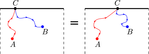
Figure 1: Path independent holonomy. The red curve corresponds to the holonomy of $A(\lambda)$ between $A$ and $C$. The blue curve corresponds to the holonomy of $A^{\beta}(-\lambda)$ between $C$ and $B$.

We can differentiate this condition and we obtain the following constraint for the Lax connection

$$\kappa(\lambda)A_{\sigma}(\lambda)-A_{\sigma}^{\beta}(-\lambda)\kappa(\lambda)\Biggr{|}_{\tau=0}=\partial_{\sigma}\kappa(\lambda).$$ (40)

This is the usual equation of the integrable boundaries, only the space and time coordinates are replaced. Some solutions which are relevant in the AdS/CFT correspondence can be found in Dekel:2011ja ; Linardopoulos:2021rfq ; Linardopoulos:2022wol .

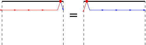
Figure 2: The $KT$-equation. The red curve corresponds to the holonomy of $A(\lambda)$ and the blue curve corresponds to the holonomy of $A^{\beta}(-\lambda)$.

Using the above defined boundary flatness condition, we can obtain the following equation (see figure 2)

$$\kappa(\lambda)T(\lambda)=T^{\beta}(-\lambda)\kappa(\lambda),$$ (41)

where $T(\lambda)$ is the monodromy matrix (9) at $\tau=0$. The equation (41) is the classical analog of the quantum $KT$-relation (2) which was introduced in Gombor:2021uxz . At this point we define two $\beta$-transformations.

1. $A^{\beta}=A$ (identity).

2. $A^{\beta}=-A^{t}$ (charge conjugation).

For the first case the $KT$-relation is simplified as

$$\kappa(\lambda)T(\lambda)=T(-\lambda)\kappa(\lambda),$$ (42)

which is the classical analog of the untwisted $KT$-relation of Gombor:2021hmj . For the second case let us introduce a new notation for the $\beta$-transformed monodromy matrix

$$\widehat{T}(\lambda):=T^{\beta}(\lambda)=\overleftarrow{\mathcal{P}\exp}\int_{\sigma=0}^{L}A_{\sigma}^{t}(\lambda)d\sigma.$$ (43)

We can see that

$$T(\lambda)\widehat{T}^{t}(\lambda)=1.$$ (44)

In the second case (where $A^{\beta}=-A^{t}$), the $KT$-relation (41) is equivalent to

$$\kappa(\lambda)T(\lambda)=\widehat{T}(-\lambda)\kappa(\lambda),$$ (45)

which is the classical analog of the twisted $KT$-relation of Gombor:2021hmj .

From the $KT$-relation and the definition of the transfer matrix (14) we can easily derive the condition

$$\mathcal{T}(\lambda)=\mathcal{T}^{\beta}(-\lambda),$$ (46)

therefore the half of the charges are vanishing which is the classical analog of integrability condition of boundary states Piroli:2017sei . Specifying the $\beta$-transformation we obtain the following conditions

$$\mathcal{T}(\lambda) =\mathcal{T}(-\lambda),$$ (47)

$$\mathcal{T}(\lambda) =\widehat{\mathcal{T}}(-\lambda),$$ (48)

which are the classical analog of the untwisted and twisted quantum integrability conditions Gombor:2020kgu .

It is worth to mention some related works. The classsical $KT$-relation (41) with some minor modifications were already appeared in Caudrelier:2014oia . This paper investigated the non-linear Schrödinger equation and introduced a dual, equal-space, Poisson bracket which describes a Hamiltonian flow in the space direction. In this dual Hamiltonian flow a usual defect in space can be considered as a defect in time. The Liouville integrability was also proved in this dual picture. These ideas have been developed along various directions and for various key models Caudrelier:2014gsa ; Avan:2015gja ; Doikou:2016oej ; Doikou:2019njk .

5 Lax description of crosscaps

In this section we can generalize the argument of the previous section for crosscap conditions (5),(6).

Now we identify the antipodal points of the time boundary $\tau=0$ therefore the flatness condition has to be modified in the following way: the holonomy

$$\left[\overleftarrow{\mathcal{P}\exp}\int_{\gamma_{2}}-A^{\beta}(-\lambda)\right]\kappa\left[\overleftarrow{\mathcal{P}\exp}\int_{\gamma_{1}}-A(\lambda)\right]$$ (49)

is independent of the path, see figure 3. The endpoints of the curves $\gamma_{1},\gamma_{2}$ are $[C,A],[B,C^{\prime}]$ where $A$ and $B$ are fixed and $C=(0,\sigma_{0}),C^{\prime}=(0,\sigma_{0}+\frac{L}{2})$. The holonomy (49) is independent from the space coordinate $\sigma_{0}$.

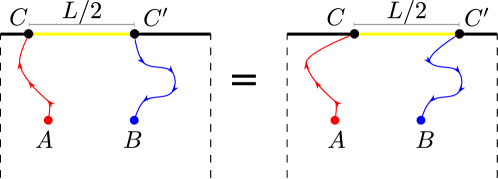
Figure 3: Path independent holonomy.

The local version of this flatness condition is

$$\kappa A_{\sigma}(\lambda)\Biggr{|}_{\tau=0,\sigma=\sigma_{0}}=A_{\sigma}^{\beta}(-\lambda)\kappa\Biggr{|}_{\tau=0,\sigma=\sigma_{0}+\frac{L}{2}}.$$ (50)

As in the previous section, we distinguish two types of automorphism $\beta$:

1. $A^{\beta}=A$ (identity).

2. $A^{\beta}=-A^{t}$ (charge conjugation).

Let us start with the first case when $\beta=\mathrm{id}$. Applying the crosscap condition twice, we obtain that

$$A_{\sigma}(\lambda)\Biggr{|}_{\tau=0,\sigma=\sigma_{0}}=\kappa^{-1}A_{\sigma}(-\lambda)\kappa\Biggr{|}_{\tau=0,\sigma=\sigma_{0}+\frac{L}{2}}=\left(\kappa^{-1}\right)^{2}A_{\sigma}(\lambda)\kappa^{2}\Biggr{|}_{\tau=0,\sigma=\sigma_{0}},$$ (51)

where we used the periodic boundary condition $\sigma\equiv\sigma+L$. Since we do not want to introduce any local constraint for the fields, the crosscap is consistent if

$$\kappa^{2}=c\mathbf{1},$$ (52)

where $c\in\mathbb{C}$. Since the flatness condition is linear in $\kappa$ we can always choose a normalization where $\kappa^{2}=\mathbf{1}$. For the second case ($\beta$ is the charge conjugation) the crosscap condition reads as

$$\kappa A_{\sigma}(\lambda)\Biggr{|}_{\tau=0,\sigma=\sigma_{0}}=-A_{\sigma}^{t}(-\lambda)\kappa\Biggr{|}_{\tau=0,\sigma=\sigma_{0}+\frac{L}{2}}.$$ (53)

Applying this crosscap condition twice, we obtain that

$$A_{\sigma}(\lambda)\Biggr{|}_{\tau=0,\sigma=\sigma_{0}}=-\kappa^{-1}A_{\sigma}^{t}(-\lambda)\kappa\Biggr{|}_{\tau=0,\sigma=\sigma_{0}+\frac{L}{2}}=\kappa^{-1}\kappa^{t}A_{\sigma}(\lambda)(\kappa^{-1})^{t}\kappa\Biggr{|}_{\tau=0,\sigma=\sigma_{0}}.$$ (54)

Similarly as in the previous case, we do not want to introduce any local constraint for the fields therefore the crosscap is consistent if

$$\kappa^{t}=\pm\kappa.$$ (55)

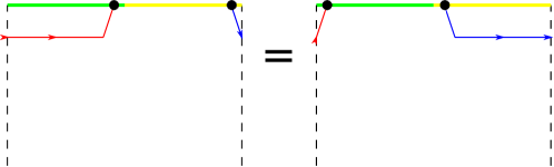
Figure 4: The $KT$-equation.

Using the global (49) or the local (50) crosscap condition of the Lax connection we can obtain the following equation (see figure 4)

$$\kappa T^{(1)}(\lambda)=T^{(2),\alpha}(-\lambda)\kappa,$$ (56)

where $T^{(1)}(\lambda),T^{(2)}(\lambda)$ are two new monodromy matrices at $\tau=0:$

$$T^{(1)}(\lambda) =\overleftarrow{\mathcal{P}\exp}\int_{0}^{L/2}-A_{\sigma}(\lambda|\tau=0,\sigma)d\sigma.$$ (57)

$$T^{(2)}(\lambda) =\overleftarrow{\mathcal{P}\exp}\int_{L/2}^{L}-A_{\sigma}(\lambda|\tau=0,\sigma)d\sigma.$$ (58)

It is obvious that the full monodromy matrix is the product of them:

$$T(\lambda)=T^{(2)}(\lambda)T^{(1)}(\lambda).$$ (59)

The equation (56) is the classical analog of the quantum $KT$-relation which was introduced in Gombor:2022deb . For the first case ($\beta$ is the identity) the $KT$-relation is simplified as

$$\kappa T^{(1)}(\lambda)=T^{(2)}(-\lambda)\kappa,$$ (60)

which is the classical analog of the untwisted $KT$-relation of Gombor:2022deb . For the second case (where $A^{\beta}=-A^{t}$) the equation (56) is equivalent to

$$\kappa T^{(1)}(\lambda)=\widehat{T}^{(2)}(-\lambda)\kappa,$$ (61)

which is the classical analog of the twisted $KT$-relation of Gombor:2022deb . Using the connection (44) between the monodromy matrices, we can obtain an equivalent form of the twisted $KT$-relation

$$\kappa^{t}T^{(2)}(\lambda)=\widehat{T}^{(1)}(-\lambda)\kappa^{t}.$$ (62)

Applying the untwisted $KT$-relation to the transfer matrix we obtain that

$$\mathcal{T}(\lambda)=\mathrm{Tr}T^{(2)}(\lambda)T^{(1)}(\lambda)=\mathrm{Tr}\kappa T^{(1)}(-\lambda)\kappa^{-1}\kappa^{-1}T^{(2)}(-\lambda)\kappa.$$ (63)

Using the constraint (52) for the untwisted $\kappa$-matrix, we just obtained that

$$\mathcal{T}(\lambda)=\mathcal{T}(-\lambda),$$ (64)

which is the classical analog of the untwisted quantum integrability condition Gombor:2022deb .

Applying the twisted $KT$-relation to the transfer matrix we obtain that

$$\mathcal{T}(\lambda)=\mathrm{Tr}T^{(2)}(\lambda)T^{(1)}(\lambda)=\mathrm{Tr}\left((\kappa^{t})^{-1}\widehat{T}^{(1)}(-\lambda)\kappa^{t}\kappa^{-1}\widehat{T}^{(2)}(-\lambda)\kappa\right).$$ (65)

Using the constraint (55) for the twisted $\kappa$-matrix, we just obtained that

$$\mathcal{T}(\lambda)=\widehat{\mathcal{T}}(-\lambda),$$ (66)

which is the classical analog of the twisted quantum integrability condition Gombor:2022deb .

Let us analyze the solutions of the crosscap conditions for the models which are described by the type of Lax pairs (17). The crosscap conditions for the currents are

$$J_{\sigma}\Biggr{|}_{\tau=0,\sigma=\sigma_{0}} =\kappa^{-1}J_{\sigma}^{\beta}\kappa\Biggr{|}_{\tau=0,\sigma=\sigma_{0}+\frac{L}{2}}=J_{\sigma}^{\alpha}\Biggr{|}_{\tau=0,\sigma=\sigma_{0}+\frac{L}{2}}$$ (67)

$$J_{\tau}\Biggr{|}_{\tau=0,\sigma=\sigma_{0}} =-\kappa^{-1}J_{\tau}^{\beta}\kappa\Biggr{|}_{\tau=0,\sigma=\sigma_{0}+\frac{L}{2}}=-J_{\tau}^{\alpha}\Biggr{|}_{\tau=0,\sigma=\sigma_{0}+\frac{L}{2}}$$ (68)

where we introduced the transformation

$$X^{\alpha}=\Omega(X):=\kappa^{-1}X^{\beta}\kappa.$$ (69)

We already saw that $\Omega^{2}=\mathrm{id}$ for the consistent crosscaps. We can see that the conditions (67),(68) are equivalent to the crosscap conditions (5),(6) therefore the construction of this section indeed describes crosscaps.

Let us decompose the current as $J_{\mu}=J_{\mu}^{(0)}+J_{\mu}^{(1)}$ where $\Omega(J_{\mu}^{(0)})=J_{\mu}^{(0)}$ and $\Omega(J_{\mu}^{(1)})=-J_{\mu}^{(1)}$. Using these notations the crosscap condition simplifies as

$$J_{\sigma}^{(0)}\Biggr{|}_{\tau=0,\sigma=\sigma_{0}} =J_{\sigma}^{(0)}\Biggr{|}_{\tau=0,\sigma=\sigma_{0}+\frac{L}{2}}, J_{\sigma}^{(1)}\Biggr{|}_{\tau=0,\sigma=\sigma_{0}} =-J_{\sigma}^{(1)}\Biggr{|}_{\tau=0,\sigma=\sigma_{0}+\frac{L}{2}},$$ (70)

$$J_{\tau}^{(1)}\Biggr{|}_{\tau=0,\sigma=\sigma_{0}} =J_{\tau}^{(1)}\Biggr{|}_{\tau=0,\sigma=\sigma_{0}+\frac{L}{2}}, J_{\tau}^{(0)}\Biggr{|}_{\tau=0,\sigma=\sigma_{0}} =-J_{\tau}^{(0)}\Biggr{|}_{\tau=0,\sigma=\sigma_{0}+\frac{L}{2}}.$$ (71)

Examples

In the following we analyze the crosscap equations (67),(68) for some concrete sigma models which were introduced in section 3. More concretely, we specify the manifestation of these crosscap equations on the concrete parametrization of the target spaces. Since we already show that the conditions (67),(68) are equivalent to the crosscap conditions (5),(6) we concentrate on the explicit forms of the $\alpha$-isometries and the corresponding residual symmetries.

Principal chiral fields

Let us concentrate on the $SU(N)$ principal chiral field i.e. $\mathfrak{g}=\mathfrak{su}(N)$. For the $\beta=\mathrm{id}$ case we have $\kappa^{2}=\mathbf{1}.$ Using the global $SU(N)$ symmetry we can diagonalize the $\kappa$-s therefore we have

$$\kappa=\mathrm{diag}(\underbrace{1,\dots,1}_{k},\underbrace{-1,\dots,-1}_{N-k}).$$ (72)

The $\alpha$-automorphism acts on the fields as $g^{\alpha}=\kappa g\kappa^{-1}$ and the residual symmetry is $SU(k)\times SU(N-k)\times U(1)$. In the second case ($\beta$ is the charge conjugation) $g^{\alpha}=\kappa\left(g^{t}\right)^{-1}\kappa^{-1}$ and the residual symmetries are $SO(N)$ or $Sp(N)$ for $\kappa=\kappa^{t}$ or $\kappa=-\kappa^{t}$, respectively.

This classification of classical crosscaps are completely analog with the classification of the crosscap states of the quantum $\mathfrak{su}(N)$ symmetric spin chains Gombor:2022deb .

$O(N)$ sigma model

For the $O(N)$ sigma model the current is an element of $\mathfrak{so}(N)$ i.e. $-J^{t}=J$ therefore only the $\beta=\mathrm{id}$ case is relevant. Since the current is anti-symmetric the consistent crosscaps require both conditions $\kappa^{2}=c\mathbf{1}$ and $\kappa^{t}=\pm\kappa$ therefore we have two classes of $\kappa$-matrices (up to global $O(N)$ rotations)

$$\kappa =\mathrm{diag}(\underbrace{1,\dots,1}_{k},\underbrace{-1,\dots,-1}_{N-k}),$$ (73)

$$\kappa =\left(\begin{array}[]{cc}0&\mathbf{1}_{\frac{N}{2}\times\frac{N}{2}}\\ -\mathbf{1}_{\frac{N}{2}\times\frac{N}{2}}&0\end{array}\right).$$ (76)

The symmetric case has residual symmetry $SO(k)\times SO(N-k)$ and the anti-symmetric one has $U(\frac{N}{2})$. In the symmetric case the solution of the equation (67) is

$$\phi_{i}^{\alpha} =\phi_{i},\qquad i=1,\dots,k,$$ (77)

$$\phi_{i}^{\alpha} =-\phi_{i},\qquad i=k+1,\dots,N.$$ (78)

For the anti-symmetric $\kappa$, the equation (67) has the solution

$$\phi_{i}^{\alpha} =-\phi_{\frac{N}{2}+i},\qquad i=1,\dots,\frac{N}{2},$$ (79)

$$\phi_{\frac{N}{2}+i}^{\alpha} =\phi_{i},\qquad i=\frac{N}{2}+1,\dots,N.$$ (80)

We can see that this is not a consistent crosscap because the square of this transformation is $-1$.

In summary, for the $O(N)$ sigma model the integrable crosscaps correspond to the residual symmetries $SO(k)\times SO(N-k)$ and the concrete identifications are given by the equations (77-78). In the table 1 we enumerate these possibilities explicitly for the $O(6)$ model.

Table 1: Crosscaps of $O(6)$ sigma model.

Residual symmetry	$(\phi_{1},\phi_{2},\phi_{3},\phi_{4},\phi_{5},\phi_{6})^{\alpha}$
$SO(6)$	$(\phi_{1},\phi_{2},\phi_{3},\phi_{4},\phi_{5},\phi_{6})$
	$(-\phi_{1},-\phi_{2},-\phi_{3},-\phi_{4},-\phi_{5},-\phi_{6})$
$SO(5)$	$(\phi_{1},\phi_{2},\phi_{3},\phi_{4},\phi_{5},-\phi_{6})$
	$(\phi_{1},-\phi_{2},-\phi_{3},-\phi_{4},-\phi_{5},-\phi_{6})$
$SO(4)\times SO(2)$	$(\phi_{1},\phi_{2},\phi_{3},\phi_{4},-\phi_{5},-\phi_{6})$
	$(\phi_{1},\phi_{2},-\phi_{3},-\phi_{4},-\phi_{5},-\phi_{6})$
$SO(3)\times SO(3)$	$(\phi_{1},\phi_{2},\phi_{3},-\phi_{4},-\phi_{5},-\phi_{6})$

Sigma model on the $AdS_{N}$

For the sigma model on the $AdS_{N}$ the current is an element of $\mathfrak{so}(2,N-1)$ i.e. $-J^{t}=\eta J\eta$ therefore only the $\beta=\mathrm{id}$ case is relevant for which we have the condition $\kappa^{2}=c\mathbf{1}$. From the crosscap equation (67) we also obtain an other constraint since $\kappa J\kappa^{-1}\in\mathfrak{so}(2,N-1)$ i.e., $\kappa^{t}=\pm\eta\kappa\eta$. Let us start with the symmetric $\kappa$-matrix

$$\kappa=\mathrm{diag}(1,1,\underbrace{1,\dots,1}_{N-2},-1).$$ (81)

This $\kappa$-matrix has $SO(2,N-2)$ symmetry. The equation (67) has the solution

$$\begin{split}X_{i}^{\alpha}&=X_{i},\qquad i=-1,\dots,N-2,\\ X_{N-1}^{\alpha}&=-X_{N-1}.\end{split}$$ (82)

Using the Poincaré coordinates we obtain that

$$\begin{split}x_{i}^{\alpha}&=\frac{x_{i}}{x^{2}+z^{2}},\qquad i=0,\dots,N-2,\\ z^{\alpha}&=\frac{z}{x^{2}+z^{2}}.\end{split}$$ (83)

Using global $SO(2,N-1)$ isometries we can rotate the $\kappa$-matrix to

$$\kappa=\mathrm{diag}(1,1,\underbrace{1,\dots,1}_{N-3},-1,1).$$ (84)

Which leads to the crosscap conditions

$$\begin{split}x_{i}^{\alpha}&=x_{i},\qquad i=0,\dots,N-3,\\ x_{N-2}^{\alpha}&=-x_{N-2},\\ z^{\alpha}&=z.\end{split}$$ (85)

Since the $\kappa$-matrices $\eqref{eq:k1}$ and $\eqref{eq:k2}$ are connected by an isometry of $AdS_{N}$ the crosscaps (83) and (85) are also equivalent up to an isometry.

The possible $\kappa^{2}=c\mathbf{1}$ matrices (up to global $SO(2,N-1)$ rotations) are

$$\kappa =\mathrm{diag}(1,1,\underbrace{1,\dots,1}_{k-1},\underbrace{-1,\dots,-1}_{N-k}),$$ (86)

$$\kappa =\mathrm{diag}(1,-1,\underbrace{1,\dots,1}_{k-1},\underbrace{-1,\dots,-1}_{N-k}),$$ (87)

where the first one has symmetry $SO(2,k-1)\times SO(N-k)$ and the second one has $SO(1,k-1)\times SO(1,N-k)$. We can also get anti-symmetric $\kappa$ but it leads to inconsistent crosscap just as for the $O(N)$ sigma model. In the first case the equation (67) has the solution

$$X_{i}^{\alpha} =X_{i},\qquad i=-1,\dots,k-2,$$ (88)

$$X_{i}^{\alpha} =-X_{i},\qquad i=k-1,\dots,N-1,$$ (89)

Using the Poincaré coordinates we obtain that

$$\begin{split}x_{i}^{\alpha}&=\frac{x_{i}}{x^{2}+z^{2}},\qquad i=0,\dots,k-2,\\ x_{i}^{\alpha}&=\frac{-x_{i}}{x^{2}+z^{2}},\qquad i=k-1,\dots,N-2,\\ z^{\alpha}&=\frac{z}{x^{2}+z^{2}}.\end{split}$$ (90)

In the boundary of $AdS$ ($z=0$) these conditions are equivalent to

$$\begin{split}x_{i}^{\alpha}&=\frac{x_{i}}{x^{2}},\qquad i=0,\dots,k-2,\\ x_{i}^{\alpha}&=\frac{-x_{i}}{x^{2}},\qquad i=k-1,\dots,N-2.\end{split}$$ (91)

For the second $\kappa$-matrix (87), we can obtain similar conditions and we show the result only in the Poincaré coordinates

$$\begin{split}x_{0}^{\alpha}&=\frac{-x_{0}}{x^{2}+z^{2}},\\ x_{i}^{\alpha}&=\frac{x_{i}}{x^{2}+z^{2}},\qquad i=1,\dots,k-2,\\ x_{i}^{\alpha}&=\frac{-x_{i}}{x^{2}+z^{2}},\qquad i=k-1,\dots,N-2,\\ z^{\alpha}&=\frac{z}{x^{2}+z^{2}}.\end{split}$$ (92)

In the boundary of $AdS$ ($z=0$) these conditions are equivalent to

$$\begin{split}x_{0}^{\alpha}&=\frac{-x_{0}}{x^{2}},\\ x_{i}^{\alpha}&=\frac{x_{i}}{x^{2}},\qquad i=1,\dots,k-2,\\ x_{i}^{\alpha}&=\frac{-x_{i}}{x^{2}},\qquad i=k-1,\dots,N-2.\end{split}$$ (93)

In summary, for the sigma model on the $AdS_{N}$ the integrable crosscaps correspond to the residual symmetries $SO(2,k-1)\times SO(N-k)$ or $SO(1,k-1)\times SO(1,N-k)$. In the tables 2 and 3 we enumerate these possibilities explicitly for the $AdS_{5}$ and $AdS_{4}$.

Table 2: Crosscaps of the sigma model on $AdS_{5}$.

Residual symmetry	$(x_{0},x_{1},x_{2},x_{3},z)^{\alpha}$
$SO(2,4)$	$(x_{0},x_{1},x_{2},x_{3},z)$
$SO(2,3)$	$\left(\frac{x_{0}}{x^{2}+z^{2}},\frac{x_{1}}{x^{2}+z^{2}},\frac{x_{2}}{x^{2}+z^{2}},\frac{x_{3}}{x^{2}+z^{2}},\frac{z}{x^{2}+z^{2}}\right)$
$SO(2,2)\times SO(2)$	$\left(\frac{x_{0}}{x^{2}+z^{2}},\frac{x_{1}}{x^{2}+z^{2}},\frac{x_{2}}{x^{2}+z^{2}},\frac{-x_{3}}{x^{2}+z^{2}},\frac{z}{x^{2}+z^{2}}\right)$
$SO(2,1)\times SO(3)$	$\left(\frac{x_{0}}{x^{2}+z^{2}},\frac{x_{1}}{x^{2}+z^{2}},\frac{-x_{2}}{x^{2}+z^{2}},\frac{-x_{3}}{x^{2}+z^{2}},\frac{z}{x^{2}+z^{2}}\right)$
$SO(2)\times SO(4)$	$\left(\frac{x_{0}}{x^{2}+z^{2}},\frac{-x_{1}}{x^{2}+z^{2}},\frac{-x_{2}}{x^{2}+z^{2}},\frac{-x_{3}}{x^{2}+z^{2}},\frac{z}{x^{2}+z^{2}}\right)$
$SO(1,4)$	$\left(\frac{-x_{0}}{x^{2}+z^{2}},\frac{-x_{1}}{x^{2}+z^{2}},\frac{-x_{2}}{x^{2}+z^{2}},\frac{-x_{3}}{x^{2}+z^{2}},\frac{z}{x^{2}+z^{2}}\right)$
$SO(1,1)\times SO(1,3)$	$\left(\frac{-x_{0}}{x^{2}+z^{2}},\frac{x_{1}}{x^{2}+z^{2}},\frac{-x_{2}}{x^{2}+z^{2}},\frac{-x_{3}}{x^{2}+z^{2}},\frac{z}{x^{2}+z^{2}}\right)$
	$\left(\frac{-x_{0}}{x^{2}+z^{2}},\frac{x_{1}}{x^{2}+z^{2}},\frac{x_{2}}{x^{2}+z^{2}},\frac{x_{3}}{x^{2}+z^{2}},\frac{z}{x^{2}+z^{2}}\right)$
$SO(1,2)\times SO(1,2)$	$\left(\frac{-x_{0}}{x^{2}+z^{2}},\frac{x_{1}}{x^{2}+z^{2}},\frac{x_{2}}{x^{2}+z^{2}},\frac{-x_{3}}{x^{2}+z^{2}},\frac{z}{x^{2}+z^{2}}\right)$

Table 3: Crosscaps of the sigma model on $AdS_{4}$.

Residual symmetry	$(x_{0},x_{1},x_{2},z)^{\alpha}$
$SO(2,3)$	$(x_{0},x_{1},x_{2},z)$
$SO(2,2)$	$\left(\frac{x_{0}}{x^{2}+z^{2}},\frac{x_{1}}{x^{2}+z^{2}},\frac{x_{2}}{x^{2}+z^{2}},\frac{z}{x^{2}+z^{2}}\right)$
$SO(2,1)\times SO(2)$	$\left(\frac{x_{0}}{x^{2}+z^{2}},\frac{x_{1}}{x^{2}+z^{2}},\frac{-x_{2}}{x^{2}+z^{2}},\frac{z}{x^{2}+z^{2}}\right)$
$SO(2)\times SO(3)$	$\left(\frac{x_{0}}{x^{2}+z^{2}},\frac{-x_{1}}{x^{2}+z^{2}},\frac{-x_{2}}{x^{2}+z^{2}},\frac{z}{x^{2}+z^{2}}\right)$
$SO(1,3)$	$\left(\frac{-x_{0}}{x^{2}+z^{2}},\frac{-x_{1}}{x^{2}+z^{2}},\frac{-x_{2}}{x^{2}+z^{2}},\frac{z}{x^{2}+z^{2}}\right)$
$SO(1,1)\times SO(1,2)$	$\left(\frac{-x_{0}}{x^{2}+z^{2}},\frac{x_{1}}{x^{2}+z^{2}},\frac{-x_{2}}{x^{2}+z^{2}},\frac{z}{x^{2}+z^{2}}\right)$
	$\left(\frac{-x_{0}}{x^{2}+z^{2}},\frac{x_{1}}{x^{2}+z^{2}},\frac{x_{2}}{x^{2}+z^{2}},\frac{z}{x^{2}+z^{2}}\right)$

Sigma model on the $\mathbb{C}\mathrm{P}^{N-1}$

For the $\mathbb{C}\mathrm{P}^{N-1}$ sigma model the current is an element of $\mathfrak{su}(N)$. For the $\beta=\mathrm{id}$ case we have $\kappa^{2}=\mathbf{1}.$ Using the global $SU(N)$ symmetry we can diagonalize the $\kappa$-s therefore we have

$$\kappa=\mathrm{diag}(\underbrace{1,\dots,1}_{k},\underbrace{-1,\dots,-1}_{N-k}).$$ (94)

This $\kappa$-matrix has residual symmetry $SU(k)\times SU(N-k)\times U(1)$. The solution of the equation (67) is

$$Y_{i}^{\alpha} =Y_{i},\qquad i=1,\dots,k,$$ (95)

$$Y_{i}^{\alpha} =-Y_{i},\qquad i=k+1,\dots,N.$$ (96)

In the second case (the charge conjugation case when $\kappa^{t}=\pm\kappa$) we have two types of $\kappa$-matrices (up to global $SU(N)$ rotations)

$$\kappa =\mathbf{1},$$ (97)

$$\kappa =\left(\begin{array}[]{cc}0&\mathbf{1}_{\frac{N}{2}\times\frac{N}{2}}\\ -\mathbf{1}_{\frac{N}{2}\times\frac{N}{2}}&0\end{array}\right).$$ (100)

The symmetric case has residual symmetry $SO(N)$ and the anti-symmetric one has $Sp(N)$. In the symmetric case the solution of the equation (67) is

$$Y_{i}^{\alpha} =\bar{Y}_{i},\qquad i=1,\dots,N,$$ (101)

where the bar denotes the complex conjugation. For the anti-symmetric $\kappa$ the equation (67) has the solution

$$Y_{i}^{\alpha} =-\bar{Y}_{\frac{N}{2}+i},\qquad i=1,\dots,\frac{N}{2},$$ (102)

$$Y_{\frac{N}{2}+i}^{\alpha} =\bar{Y}_{i},\qquad i=\frac{N}{2}+1,\dots,N.$$ (103)

We can see that this is not a consistent crosscap because the square of this transformation is $-1$.

In summary, for the $\mathbb{C}\mathrm{P}^{N-1}$ sigma model the integrable crosscaps correspond to the residual symmetries $SU(k)\times SU(N-k)\times U(1)$ or $SO(N)$ and the concrete identifications are given by the equations (95-96) or (101). In the table 4 we enumerate these possibilities explicitly for the $\mathbb{C}\mathrm{P}^{3}$ .

Table 4: Crosscaps of $\mathbb{C}\mathrm{P}^{3}$ sigma model.

Residual symmetry	$(Y_{1},Y_{2},Y_{3},Y_{4})^{\alpha}$
$SU(4)$	$(Y_{1},Y_{2},Y_{3},Y_{4})$
	$(-Y_{1},-Y_{2},-Y_{3},-Y_{4})$
$SU(3)\times U(1)$	$(Y_{1},Y_{2},Y_{3},-Y_{4})$
	$(Y_{1},-Y_{2},-Y_{3},-Y_{4})$
$SU(2)\times SU(2)\times U(1)$	$(Y_{1},Y_{2},-Y_{3},-Y_{4})$
$SO(4)$	$(-\bar{Y}_{3},-\bar{Y}_{4},\bar{Y}_{1},\bar{Y}_{2})$

6 Crosscaps in the AdS/CFT duality

In this section we apply the results of the previous sections to the classical sigma models which are relevant in the $AdS_{5}/CFT_{4}$ and the $AdS_{4}/CFT_{3}$ dualities. The string theory side we have type IIB superstrings on the $AdS_{5}\times S^{5}$ and type IIA superstrings on the $AdS_{4}\times\mathbb{CP}^{3}$. The dual field theories are the $\mathcal{N}=4$ SYM and the ABJM theories. The isometries of the $AdS$ and the $S^{5}$ (or $\mathbb{CP}^{3}$) correspond to the conformal symmetries and the $R$-symmetries of the field theories. In the following we also use the latter names for the isometries of the target spaces.

In the following, we classify the integrable crosscaps of classical sigma models corresponding these superstrings, but we also make a few physically reasonable restrictions. We concentrate on the half-BPS crosscaps. Furthermore, we require some breaking of the conformal symmetry since otherwise they would not be non-vanishing one-point functions. On the other hand we want the dilation operator to be unbroken, in other words, the residual symmetry should contain a lower-dimensional conformal symmetry group.

6.1 $AdS_{5}/CFT_{4}$

In this subsection we classify the integrable crosscaps for type IIB strings on the $AdS_{5}\times S^{5}$. The classical string can be described as a sigma model on the supercoset Metsaev:1998it

$$\frac{PSU(2,2|4)}{SO(1,4)\times SO(5)}.$$ (104)

We can define the current in the usual way $J=g^{-1}dg$ where $g(\tau,\sigma)\in PSU(2,2|4)$. The superalgebra $\mathfrak{psu}(2,2|4)$ has a $\mathbb{Z}_{4}$ automorphism for which the current decomposes as $J=J^{(0)}+J^{(1)}+J^{(2)}+J^{(3)}$. We can define the fixed frame currents as $j^{(m)}=gJ^{(m)}g^{-1}$. The Lax pair can be written as Dekel:2011ja

$$A(\lambda)=(\lambda-1)j^{(1)}+\frac{1}{2}(\lambda-\lambda^{-1})^{2}j^{(2)}+(\lambda^{-1}-1)j^{(3)}-\frac{1}{2}(\lambda^{2}-\lambda^{-2})*j^{(2)}.$$ (105)

The theory has global $PSU(2,2|4)$ symmetry which acts on the group element as $g\to\bar{g}g$ where $\bar{g}\in PSU(2,2|4)$ is a constant group element. The current $J$ is invariant under this transformation however the fixed frame currents transform as $j^{(m)}\to\bar{g}j^{(m)}\bar{g}^{-1}$ therefore the Lax connection also transforms as

$$A(\lambda)\to\bar{g}A(\lambda)\bar{g}^{-1}.$$ (106)

Let us continue with the crosscap condition (50). At first let $A^{\beta}(\lambda)=A(\lambda)$ therefore

$$A_{\sigma}(\lambda)\Biggr{|}_{\tau=0,\sigma=\sigma_{0}}=\kappa^{-1}A_{\sigma}(-\lambda)\kappa\Biggr{|}_{\tau=0,\sigma=\sigma_{0}+\frac{L}{2}}.$$ (107)

Applying the transformation (106), we obtain that

$$A_{\sigma}(\lambda)\Biggr{|}_{\tau=0,\sigma=\sigma_{0}}=\bar{g}^{-1}\kappa^{-1}\bar{g}A_{\sigma}(-\lambda)\bar{g}^{-1}\kappa\bar{g}\Biggr{|}_{\tau=0,\sigma=\sigma_{0}+\frac{L}{2}}.$$ (108)

We can see that this condition breaks the global $PSU(2,2|4)$ symmetry, the residual symmetry is defined by

$$\bar{g}^{-1}\kappa\bar{g}=\kappa.$$ (109)

We saw that, the consistency of the crosscap requires that $\kappa^{2}=\mathbf{1}$ therefore the possible $\kappa$-s (up to global rotations) are

$$\kappa=\mathrm{diag}(\underbrace{1,\dots,1}_{k},\underbrace{-1,\dots,-1}_{4-k}|\underbrace{-1,\dots,-1}_{4-l},\underbrace{1,\dots,1}_{l}).$$ (110)

Let us forget about the signature for a moment. The $\kappa$-matrix breaks the global symmetry $\mathfrak{gl}(4|4)$ to $\mathfrak{gl}(k|l)\oplus\mathfrak{gl}(4-k|4-l)$ (up to $\mathfrak{u}(1)$ factors). Let us concentrate on the 1/2 BPS configurations. We have three possibilities

$$\mathfrak{gl}(2|2)\oplus\mathfrak{gl}(2|2),\qquad\mathfrak{gl}(2|4)\oplus\mathfrak{gl}(2),\qquad\mathfrak{gl}(4|2)\oplus\mathfrak{gl}(2),\qquad\mathfrak{gl}(3|2)\oplus\mathfrak{gl}(1|2)$$ (111)

The last possibility contains bosonic subalgebra $\mathfrak{u}(3)$ but we already show that this symmetry has no consistent crosscap for the sigma models neither on the $S^{5}$ or the $AdS_{5}$. The $\mathfrak{gl}(4|2)\oplus\mathfrak{gl}(2)$ case preserves the full conformal symmetry $SO(2,4)$ which means there cannot be non-vanishing one-point function in the CFT side therefore we neglect this case. We can see that only the first two possibilities remain.

• For the $\mathfrak{gl}(2|2)\oplus\mathfrak{gl}(2|2)$ case the conformal symmetry breaks as $SO(2,4)\to SO(2,2)\times SO(2)$ or $SO(2)\times SO(4)$ and we already derived which are the corresponding crosscap conditions on the Poincaré patch, see table 2. The $R$-symmetry breaks as $SO(6)\to SO(2)\times SO(4)$ and we already derived which are the corresponding crosscap conditions on the sphere, see table 1.

• For the $\mathfrak{gl}(2|4)\oplus\mathfrak{gl}(2)$ case the conformal symmetry breaks as $SO(2,4)\to SO(2,2)\times SO(2)$ or $SO(2)\times SO(4)$ and the $R$-symmetry is unbroken.

Let us continue with the the crosscap conditions (50) with the transformation $A^{\beta}(\lambda)=-M^{-1}A(\lambda)^{st}M$ where

$$M=\left(\begin{array}[]{ccc}\mathbf{1}_{4\times 4}&0&0\\ 0&0&\mathbf{1}_{2\times 2}\\ 0&-\mathbf{1}_{2\times 2}&0\end{array}\right),$$ (112)

and the super-transposition $\>{}^{st}$ acts in the usual way

$$\left(\begin{array}[]{cc}A&Q\\ S&B\end{array}\right)^{st}=\left(\begin{array}[]{cc}A^{t}&-S^{t}\\ Q^{t}&B^{t}\end{array}\right),$$ (113)

where $A,B$ and $Q,S$ are $4\times 4$ bosonic and fermionic matrices. Using these definitions we can show that the $\beta$ is a $\mathbb{Z}_{2}$ automorphism of $\mathfrak{gl}(4|4)$. The crosscap conditions read as

$$A_{\sigma}(\lambda)\Biggr{|}_{\tau=0,\sigma=\sigma_{0}}=-\kappa^{-1}M^{-1}A_{\sigma}(-\lambda)^{st}M\kappa\Biggr{|}_{\tau=0,\sigma=\sigma_{0}+\frac{L}{2}}.$$ (114)

Applying this transformation twice we obtain that

$$A_{\sigma}(\lambda)=\kappa^{-1}M^{-1}(\kappa^{-1}M^{-1}A_{\sigma}(\lambda)^{st}M\kappa)^{st}M\kappa.$$ (115)

For bosonic $\kappa$-matrix, we obtain that

$$A_{\sigma}(\lambda)=\kappa^{-1}M^{-1}\kappa^{t}MM^{-1}(M^{-1}A_{\sigma}(\lambda)^{st}M)^{st}MM^{-1}\left(\kappa^{-1}\right)^{t}M\kappa=\\ \left(\kappa^{-1}M^{-1}\kappa^{t}M\right)A_{\sigma}(\lambda)\left(M^{-1}\left(\kappa^{-1}\right)^{t}M\kappa\right),$$ (116)

where we used the identity

$$M^{-1}(M^{-1}A_{\sigma}(\lambda)^{st}M)^{st}M=A_{\sigma}(\lambda).$$

For a consistent crosscap we obtained the following constraint for the $\kappa$-matrix

$$\kappa=\pm M^{-1}\kappa^{t}M.$$ (117)

We have two types of $\kappa$-matrices (up to global rotations). For the $+$ sign the $\kappa$-matrix reads as

$$\kappa=\mathbf{1},$$ (118)

and for the $-$ sign the $\kappa$-matrix is

$$\kappa=\left(\begin{array}[]{cccc}0&\mathbf{1}_{2\times 2}&0&0\\ -\mathbf{1}_{2\times 2}&0&0&0\\ 0&0&0&-\mathbf{1}_{2\times 2}\\ 0&0&\mathbf{1}_{2\times 2}&0\end{array}\right).$$ (119)

Applying the transformation (106), we obtain that

$$A_{\sigma}(\lambda)\Biggr{|}_{\tau=0,\sigma=\sigma_{0}}=\bar{g}^{-1}\kappa^{-1}M^{-1}\left(\bar{g}^{-1}\right)^{st}A_{\sigma}(-\lambda)^{st}\bar{g}^{st}M\kappa\bar{g}\Biggr{|}_{\tau=0,\sigma=\sigma_{0}+\frac{L}{2}}.$$ (120)

We can see that this condition breaks the global $PSU(2,2|4)$ symmetry and the residual symmetry is defined by

$$\bar{g}^{st}M\kappa\bar{g}=M\kappa.$$ (121)

We already saw that, for a consistent crosscap we have two types of $\kappa$-matrices. For the symmetric $\kappa$-matrix (118) we have

$$M\kappa=M=\left(\begin{array}[]{ccc}\mathbf{1}_{4\times 4}&0&0\\ 0&0&\mathbf{1}_{2\times 2}\\ 0&-\mathbf{1}_{2\times 2}&0\end{array}\right)$$ (122)

for which the residual symmetry is $\mathfrak{osp}(4|4)$. For the anti-symmetric $\kappa$-matrix (118) we have

$$M\kappa=\left(\begin{array}[]{ccc}0&\mathbf{1}_{2\times 2}&0\\ -\mathbf{1}_{2\times 2}&0&0\\ 0&0&\mathbf{1}_{4\times 4}\end{array}\right)$$ (123)

for which the residual symmetry is also $\mathfrak{osp}(4|4)$ but now the first $4\times 4$ bosonic block breaks to $\mathfrak{sp}(4)$ and second breaks to $\mathfrak{so}(4)$. For the sake of clarity, we denote this residual symmetry as $\mathfrak{spo}(4|4)$.

We can see that these are 1/2 BPS crosscaps. In summary we have two possibilities:

• For the $\mathfrak{osp}(4|4)$ residual symmetry, the conformal symmetry breaks as $SO(2,4)\to SO(2,1)\times SO(3)$ and $R$-symmetry breaks as $SO(6)\to SO(5)$.

• For the $\mathfrak{spo}(4|4)$ residual symmetry, the conformal symmetry breaks as $SO(2,4)\to SO(2,3)$ and $R$-symmetry breaks as $SO(6)\to SO(3)\times SO(3).$

In the table 5 we summarized the crosscaps for the sigma model on the coset (104). This table shows the residual symmetries of the possible crosscaps and the concrete realizations (which is given by the $\mathbb{Z}_{2}$ automorphism) on the $AdS_{5}$ and the $S^{5}$ are given by the tables 2 and 1.

Table 5: Possible crosscaps in the $AdS_{5}/CFT_{4}$

Residual symmetry	Residual isometries on $AdS_{5}$	Residual isometries on $S^{5}$
$\mathfrak{gl}(2|2)\oplus\mathfrak{gl}(2|2)$	$SO(2,2)\times SO(2)$	$SO(4)\times SO(2)$
	$SO(2)\times SO(4)$
$\mathfrak{gl}(2|4)\oplus\mathfrak{gl}(2)$	$SO(2,2)\times SO(2)$	$SO(6)$
	$SO(2)\times SO(4)$
$\mathfrak{osp}(4|4)$	$SO(2,1)\times SO(3)$	$SO(5)$
	$SO(2,3)$	$SO(3)\times SO(3)$

Table 6: Possible crosscaps in the $AdS_{4}/CFT_{3}$

Residual symmetry	Residual isometries of $AdS_{4}$	Residual isometries of $\mathbb{CP}^{3}$
$\mathfrak{osp}(3|2)\oplus\mathfrak{osp}(3|2)$	$SO(2,2)$	$SO(4)$
$\mathfrak{osp}(6|2)\oplus\mathfrak{sp}(2)$	$SO(2,2)$	$SU(4)$
$\mathfrak{osp}(4|2)\oplus\mathfrak{osp}(2|2)$	$SO(2,2)$	$SU(2)\times SU(2)\times U(1)$
$\mathfrak{gl}(3|2)$	$SO(2,1)\times SO(2)$	$SU(3)\times U(1)$

6.2 $AdS_{4}/CFT_{3}$

In this subsection we classify the integrable crosscaps for type IIA superstrings on $AdS_{4}\times\mathbb{CP}^{3}$. The classical string can be described as a sigma model on the supercoset Arutyunov:2008if

$$\frac{OSP(6|4)}{SO(1,3)\times U(3)}.$$ (124)

We can define the current in the usual way $J=g^{-1}dg$ where $g(\tau,\sigma)\in OSP(6|4)$. We can also define the fixed frame currents and Lax connect operators in the same way as before (105). We saw that the consistency of the crosscap requires that $\kappa^{2}=\mathbf{1}$ and now the current has the symmetry $J=-VJ^{st}V^{-1}$where

$$V=\left(\begin{array}[]{ccc}\mathbf{1}_{6\times 6}&0&0\\ 0&0&\mathbf{1}_{2\times 2}\\ 0&-\mathbf{1}_{2\times 2}&0\end{array}\right),$$ (125)

therefore the consistency also requires that $\kappa^{t}=\pm V\kappa V^{-1}$ (the $\kappa$-matrix is bosonic). The theory has global $OSP(6|4)$ symmetry which act on the group element as $g\to\bar{g}g$ where $\bar{g}\in OSP(6|4)$ is a constant group element. Repeating the argument of the previous subsection we obtain that the residual symmetry is defined by

$$\bar{g}^{-1}\kappa\bar{g}=\kappa.$$ (126)

The type $\kappa^{t}=+V\kappa V^{-1}$ matrices can be written (up to global rotations) as

$$\kappa=\mathrm{diag}(\underbrace{1,\dots,1}_{k},\underbrace{-1,\dots,-1}_{6-k}|\underbrace{-1,\dots,-1}_{\frac{l}{2}},\underbrace{1,\dots,1}_{\frac{4-l}{2}},\underbrace{-1,\dots,-1}_{\frac{l}{2}},\underbrace{1,\dots,1}_{\frac{4-l}{2}}).$$ (127)

This $\kappa$-matrix breaks the global symmetry $\mathfrak{osp}(6|4)$ to $\mathfrak{osp}(k|l)\oplus\mathfrak{osp}(6|4-l)$. Let us concentrate on the 1/2 BPS configurations. We have five possibilities

$$\mathfrak{osp}(3|2)\oplus\mathfrak{osp}(3|2),\quad\mathfrak{osp}(6|2)\oplus\mathfrak{sp}(2),\quad\mathfrak{osp}(3|4)\oplus\mathfrak{so}(3),\quad\mathfrak{osp}(4|2)\oplus\mathfrak{osp}(2|2),\quad\mathfrak{osp}(5|2)\oplus\mathfrak{osp}(1|2).$$

In the last possibility the $R$-symmetry breaks as $\mathfrak{su}(4)\to\mathfrak{so}(5)\cong\mathfrak{sp}(4)$ but we already showed that this symmetry has no consistent crosscap for the sigma model on $\mathbb{CP}^{3}$. The $\mathfrak{osp}(3|4)\oplus\mathfrak{so}(3)$ case preserves the full conformal symmetry $SO(2,3)$ which means there cannot be non-vanishing one-point function in the CFT side therefore we neglect this case. We can see that three possibilities remain.

• For the $\mathfrak{osp}(3|2)\oplus\mathfrak{osp}(3|2)$ case the conformal symmetry breaks as $SO(2,3)\to SO(2,2)$ and we already derived which are the corresponding crosscap conditions on the Poincaré patch, see table 3. The $R$-symmetry breaks as $SU(4)\to SO(4)$ and we already derived which are the corresponding crosscap conditions on the $\mathbb{CP}^{3}$, see table 4.

• For the $\mathfrak{osp}(6|2)\oplus\mathfrak{sp}(2)$ case the conformal symmetry breaks as $SO(2,3)\to SO(2,2)$ and the $R$-symmetry is preserved.

• For the $\mathfrak{osp}(4|2)\oplus\mathfrak{osp}(2|2)$ case the conformal symmetry breaks as $SO(2,3)\to SO(2,2)$ and the $R$-symmetry breaks as $SU(4)\to SU(2)\times SU(2)\times U(1)$.

The type $\kappa^{t}=-V\kappa V^{-1}$ matrices can be written (up to global rotations) as

$$\kappa=\left(\begin{array}[]{cccc}0&\mathbf{1}_{3\times 3}&0&0\\ -\mathbf{1}_{3\times 3}&0&0&0\\ 0&0&\mathbf{1}_{2\times 2}&0\\ 0&0&0&-\mathbf{1}_{2\times 2}\end{array}\right).$$ (128)

This $\kappa$-matrix breaks the global symmetry $\mathfrak{osp}(6|4)$ to $\mathfrak{gl}(3|2)$ which is 1/2 BPS. The conformal symmetry breaks as $SO(2,3)\to SO(2,1)\times SO(2)$ and the $R$-symmetry breaks as $SU(4)\to SU(3)\times U(1)$.

In the table 6 we summarized the crosscaps for the sigma model on the coset (124). This table shows the residual symmetries of the possible crosscaps and the concrete realizations (which is given by the $\mathbb{Z}_{2}$ automorphism) on the $AdS_{4}$ and the $\mathbb{CP}^{3}$ are given by the tables 3 and 4.

6.3 Crosscaps at weak coupling

In the literature there is an other classification of crosscaps which is relevant in the field theory side Gombor:2022deb . This paper contains the classifications of crosscap states of $SO(6)$ and the alternating $SU(4)$ spin chains which describes the $\mathcal{N}=4$ SYM and ABJM theories at weak coupling. In this paper we used such parametrization of the bosonic spaces which can be directly match to the CFT side of the duality. The $S^{5}$ and $\mathbb{C}\mathrm{P}^{3}$ are parameterized with the coordinates $(\phi_{1},\phi_{2},\dots,\phi_{6})$ and $(Y_{1},Y_{2},Y_{3},Y_{4})$ which corresponds to the scalar field of the $\mathcal{N}=4$ SYM and ABJM theories. The corresponding $\mathbb{Z}_{2}$ isometries can be found in the tables 1 and 4. We can compare the proposed crosscaps at strong coupling (result of this paper) and at weak coupling (result of Gombor:2022deb ) and we find that they are almost the same. There are two differences. There is no $U(3)$ symmetric crosscap for the $S^{5}$ sigma model and there is no $Sp(4)$ symmetric crosscap for the $\mathbb{C}\mathrm{P}^{3}$ sigma model.

The spin chain classifications belong only to the scalar sectors and they tell nothing about the effect of the crosscap on the spacetime. The main advantage of the analysis of this paper is the following. The classification of the crosscaps of the sigma models on the supercosets tells us what are the consistent combinations of the crosscaps on the $AdS_{5}$ (or $AdS_{4}$) and the $S^{5}$ (or $\mathbb{C}\mathrm{P}^{3}$), see tables 5 and 6. Therefore we obtained candidates for the crosscaps on the $CFT$ side of the duality. In the tables 2 and 3 we can find the possible crosscaps of $AdS_{5}$ and $AdS_{4}$ which are parameterized with the Poincaré coordinates $(z,x_{0},x_{1},\dots)$ therefore we can obtain the identifications of the spacetime of the $\mathcal{N}=4$ SYM and ABJM by taking the limit $z=0$.

In summary we obtained propositions for the possible integrable crosscaps of $\mathcal{N}=4$ SYM and ABJM theories. The residual symmetries are listed in the tables 5 and 6. Each symmetry classes define identifications on the spacetime and the scalar fields. For each symmetry classes the corresponding identifications of the spacetime and scalar fields can be found in the tables 1-4 (take the $z=0$ limit). We emphasize that this classification is a conjecture for the $\mathcal{N}=4$ SYM and ABJM theories and this paper is not intended to provide a concrete field theory description (if that is even possible).

7 Conclusion

In this paper we generalized the Lax description of the sigma models with boundaries in time. For the usual local boundary conditions we obtained constraints for the classical monodromy and transfer matrices and these are the classical analogs of the $KT$-relations Gombor:2021hmj and the integrability conditions Piroli:2017sei of the quantum theories. We also generalized this framework for the crosscaps where the classical analogs of the $KT$-relations Gombor:2022deb and the integrability conditions are also appeared.

Based on this framework, we classified the integrable crosscaps for the sigma models with target spaces $SU(N)$, $S^{N-1}$, $AdS_{N-1}$ and $\mathbb{C}\mathrm{P}^{N-1}$. The classification is based on the possible residual symmetries of the crosscaps. We gave the defining isometries of the crosscaps for each residual symmetry classes. We also investigated the supercosets which are relevant in the $AdS_{5}/CFT_{4}$ and the $AdS_{4}/CFT_{3}$ dualities. We classified the integrable 1/2 BPS crosscaps based on the residual symmetries (see tables 5 and 6). The corresponding defining isometries of the bosonic subspaces can be found in the tables 1-4. It is important to emphasize that this classification only applies to classical sigma models, and at this point we do not know that which versions have consistent holographic descriptions. This is an interesting question for a future research.