Searching for H_α-emitting sources in the gaps of five transitional disks

Abstract

Context. (Pre-)Transitional disks show gaps and cavities that can be related to ongoing planet formation. According to theory, young embedded planets can accrete material from the circumplanetary and circumstellar disks and can be detected using accretion tracers, such as the H_α emission line.

Aims. We aim to detect accreting protoplanets within the cavities of five (pre-)transitional disks through adaptive-optics(AO)-assisted spectral angular differential imaging in the optical regime.

Methods. We performed simultaneous AO observations in the H_α line and the adjacent continuum using the Spectro-Polarimetric High-contrast Exoplanet REsearch (SPHERE) with the Zurich Imaging Polarimeter (ZIMPOL) at the Very Large Telescope (VLT). We combined spectral and angular differential imaging techniques to increase the contrast in the innermost regions close to the star and search for the signature of young accreting protoplanets.

Results. The reduced images show no clear H_α point source around any of the targets. We report the presence of faint H_α emission around TW Hya and HD163296: while the former is most probably an artifact related to a spike, the nature of the latter remains unclear. The spectral and angular differential images yield contrasts of 6–8 magnitudes at $\sim$100 mas from the central stars, except in the case of LkCa15, with values of $\sim$3 mag. We used the contrast curves to estimate average upper limits to the H_α line luminosity of $L_{\rm H_{\alpha}}\sim$ 5$\times$10^-6 $L_{\odot}$ at separations $\geq$200 mas for TW Hya, RXJ1615, and T Cha, while for HD163296 and LkCa15 we derive values of $\sim 3\times$10^-5 $L_{\odot}$. We estimated upper limits to the accretion luminosity of potential protoplanets, obtaining that planetary models provide an average value of $L_{\rm acc}\sim 10^{-4}$ $L_{\odot}$ at 200 mas, which is about two orders of magnitude higher than the $L_{\rm acc}$ estimated from the extrapolation of the $L_{H_{\alpha}}$ – $L_{acc}$ stellar relationship.

Conclusions. When considering all the objects observed with SPHERE/ZIMPOL in the H_α line, 5 in this work and 13 from the literature, we can explain the lack of protoplanet detections by a combination of factors, such as a majority of low-mass, low-accreting planets; potential episodic accretion; significant extinction from the circumstellar and circumplanetary disks; and the fact that the contrast is less favorable at separations of smaller than 100 mas, where giant planets are more likely to form.

1 Introduction

Circumstellar disks are the cradle of planetary systems. High-angular-resolution observations of these disks have revealed a plethora of structures, including spiral arms, warps, gaps, and radial streams that might be related to ongoing planetary formation (e.g. Andrews et al., 2011; Mayama et al., 2012; Grady et al., 2013; Boccaletti et al., 2013; Pinilla et al., 2015; Benisty et al., 2015; Pérez et al., 2016). Great efforts have been made to detect protoplanets embedded in these disks using different observational techniques. As a result, there are now two confirmed protoplanets around the star PDS 70 (Keppler et al., 2018; Mesa et al., 2019a), one around AB Aur (Currie et al., 2022), and a significant number of candidates (e.g., Biller et al., 2014; Reggiani et al., 2018; Tsukagoshi et al., 2019; Boccaletti et al., 2020; Pinte et al., 2020).

Planet-formation theories predict that embedded giant planets are surrounded by circumplanetary disks (CPDs) from which they accrete material (e.g., Lovelace et al., 2011; Gressel et al., 2013; Szulágyi et al., 2014). The accretion of matter can take place via different mechanisms. For example, in the presence of a magnetic field, magnetospheric accretion could work as in the case of low-mass stars (Lovelace et al., 2011; Zhu, 2015). In this scenario, the material is expected to reach the planet surface following the magnetic field lines. Another mechanism is “boundary layer accretion” (e.g., Owen & Menou, 2016), whereby material is accreted directly onto the planet and its CPD from the circumstellar disk (e.g., Szulágyi et al., 2014). Regardless of the mechanism, one consequence of the accretion process is the presence of shocks on the planet surface and/or the CPD that can emit accretion tracers such as the H_α emission line. Furthermore, several studies have suggested that giant accreting protoplanets could be detected using such tracers, particularly the H_α emission line (e.g., Close et al., 2014; Zhu, 2015; Szulágyi & Ercolano, 2020).

Close et al. (2014) presented the first high-angular-resolution H_α imaging observations of a young star, HD142527, and reported the detection of a H_α-emitting low-mass star embedded in its transitional disk, although the stellar or planetary nature of this latter source is a matter of ongoing discussion (Brittain et al., 2020). Since then, several works have focused on detecting accreting protoplanets through H_α imaging and/or spectro-astrometry, with the main targets being young stars surrounded by transitional disks (see e.g., Sallum et al., 2015; Whelan et al., 2015; Huélamo et al., 2018; Mendigutía et al., 2018; Cugno et al., 2019; Zurlo et al., 2020; Uyama et al., 2020; Xie et al., 2020). Currently, there are two bona fide accreting protoplanets detected in the H_α line: PDS70 b and c (Wagner et al., 2018; Haffert et al., 2019). In parallel, several works have presented simulations to derive crucial accretion parameters from H_α luminosities and line profiles (e.g., Aoyama et al., 2018; Thanathibodee et al., 2019; Marleau et al., 2022).

Here we present the main results from a project designed to detect young accreting protoplanets within the gaps of five (pre-)transitional disks with the Spectro-Polarimetric High-contrast Exoplanet REsearch (SPHERE) and the Zurich Imaging Polarimeter (ZIMPOL) at the Very Large Telescope (VLT), which complements previous works by Cugno et al. (2019) and Zurlo et al. (2020). Section 2 provides information about the five observed targets, while Sections 3 and 4 describe the data reduction and analysis. We present the main results and conclusions in the last two sections.

2 The targets

For this project, we selected young stars displaying structures in their disks, mainly gaps, as signposts of planet formation. We required that most of the gaps be spatially resolved by the instrument SPHERE/ZIMPOL (see Section 3), and that the central objects be sufficiently bright ($R\lesssim$ 12 mag) to close the loop with Sphere AO for eXoplanet Observation (SAXO), the adaptive optics (AO) module of SPHERE.

As explained above, the selected targets complement previous surveys performed with SPHERE/ZIMPOL: Cugno et al. (2019) presented observations of six stars, four of them being intermediate-mass stars (spectral types between B9 and F6) observed as part of the Guaranteed Time Observation (GTO) program of the SPHERE consortium. These authors also included data for TW Hya (program 096.C-0267B , PI. Huélamo) obtained under poor atmospheric conditions, and from the star LkCa15 obtained as part of the “Science Verification” of the instrument. Finally, Cugno et al. (2019) reanalyzed the data from the A8-type star MWC758 presented by Huélamo et al. (2018). Also, Zurlo et al. (2020) presented data for 11 additional transitional disks within 200 pc and observable with SPHERE.

Here, we present observations of four T Tauri stars (RXJ1615, LkCa15, TW Hya, T Cha) and a Herbig Ae/Be star (HD 163296). As explained above, LkCa15 (Science Verification, P.I. Huélamo) and TW Hya were previously observed by SPHERE, but under poor atmospheric conditions. The main properties of the stellar sample are summarized in Table 1. We briefly describe the targets in the following subsections. We note that we have updated all the angular separations provided using the GAIA EDR3 distances (Gaia Collaboration et al., 2016, 2021) included in Table 1.

Table 1: Properties of the observed sample

Target	$R$	$A_{\rm V}$	$T_{\rm eff}$	distance1	$M_{*}$	$L_{*}$	$R_{*}$	Age
	(mag)	(mag)	(K)	[pc]	($M_{\odot}$)	($L_{\odot}$)	($R_{\odot}$)	(Myr)
RXJ1615	11.2	0.62	40002	155.6$\pm$0.6	0.6$\pm$0.13	0.90$\pm$0.023	2.0†	1.03
LkCa15	11.6	0.62	48002	157.2$\pm$0.6	1.2$\pm$0.13	1.11$\pm$0.043	1.5†	6.33
TW Hya	10.6	0.02	40002	60.1$\pm$0.1	0.8$\pm$0.13	0.33$\pm$0.23	1.2†	6.33
T Cha	10.4	1.24	54005	102.7$\pm$0.3	1.5$\pm$0.25,6	2.55	1.8†	5${}^{+3}_{-2}$ 7
HD 163296	6.9	0.08	87508	100.9$\pm$0.4	1.91${}^{+0.12}_{-0.0}$ 8	15.5${}^{+1.5}_{-}$ 8	1.708	108

Note: ¹ GAIA EDR3 distances (Gaia Collaboration et al., 2021); ² Garufi et al. (2018); ³ Adopted from Asensio-Torres et al. (2021); ⁴ Cahill et al. (2019); ⁵ Schisano et al. (2009), estimated for a distance of 100 pc; ⁶ Huélamo et al. (2015); ⁷ Dickson-Vandervelde et al. (2021); ⁸ Guzmán-Díaz et al. (2021); ^† Estimated from $T_{\rm eff}$ and $L_{*}$.

Table 2: Observing log

Target	Obs. Date	DIT	Total Exptime	Field Rotation	Airmass∗	DIMM $\tau_{0}^{*}$
		[sec]	[sec]	[degrees]		[ms]
RXJ1615	2018 Apr 20	60	7200	123.2	1.02	8
LkCa15	2018 Dec 19	80	6720	33.9	1.48	4
TW Hya	2019 Mar 15	80	6720	107.6	1.02	5
T Cha	2019 Mar 22	70	6300	29.3	1.74	9
HD 163296†	2018 Aug 18	20	4400	7.8	1.06	7
HD 163296	2018 Sep 06	20	5100	8.9	1.15	6

Note: ^∗Average value along the exposure.

2.1 RXJ1615.3-3255

RXJ1615.3-3255 (RXJ1615 hereafter) is a member of the Lupus star forming region, and was identified as a T Tauri star (TTS) in a X-ray survey with the ROSAT satellite (Krautter et al., 1997). Analysis of Spitzer spectroscopy suggested that RXJ1615 was surrounded by a transitional disk (Merín et al., 2010), which was spatially resolved at 880 $\mu$m by the Submillimeter Array (SMA) revealing a dust cavity of $\sim$25 au in size, and a disk inclination of $\sim$41$\degree$ (Andrews et al., 2011). Later, van der Marel et al. (2015) presented resolved images of the disk using ALMA Band 9 observations (440 $\mu$m). These authors reported a smaller dust cavity ($\sim$17 au), and the presence of a second dust cavity in the outer part of the disk, between $\sim$ 0$\aas@@fstack{\prime\prime}$6 and 0$\aas@@fstack{\prime\prime}$7 (93-109 au).

de Boer et al. (2016) obtained polarimetric observations of the target with VLT/SPHERE in the optical and near-infrared (NIR) regime, which were sensitive to small dust particles in the disk surface. The images revealed a complex disk architecture with the presence of two arcs, two rings, an outer gap at $\sim$0$\aas@@fstack{\prime\prime}$5 ($\sim$78 au), and an inner disk. These authors only reported marginal evidence for an inner cavity of 25 au. They also looked for close companions, detecting nine objects between two and eight arcseconds, outside the disk. Four of these were confirmed as background sources, while the other five require additional data in order to confirm or reject them as co-moving companions. Willson et al. (2016) also looked for close companions around RXJ1615 through sparse aperture masking $K$-band observations. Although these latter authors detected a significant asymmetry in the closure phases, the identification of systematic effects on their data prevented them from drawing firm conclusions about the presence of potential companions.

Avenhaus et al. (2018) presented SPHERE/IRDIS polarimetric differential imaging of the disk in the $J$ and $H$ bands. The results obtained by these authors suggested a smaller inner cavity than that reported by van der Marel et al. (2015), as they detected scattered light down to $\sim$0$\aas@@fstack{\prime\prime}$1 (15.6 au), which corresponds to the edge of the used coronograph. By modeling the inner cavity, Asensio-Torres et al. (2021) estimated that a planet with $\sim$4.5 M_Jup at 22 au might have carved the observed gap, but they could not detect it.

2.2 LkCa 15

LkCa15 is surrounded by a pre-transitional disk with an inner disk, a large gap with a minimum at $\sim$43 au, and an outer disk at 58 au (Thalmann et al., 2016). This TTS was studied by Kraus & Ireland (2012) through SAM interferometry in the NIR, reporting the detection of a planet candidate in the gap of the disk (LkCa15b). Sallum et al. (2015) confirmed the detection of this IR signal with new SAM IR data. These authors also detected two additional IR point-like sources (LkCa15 c and d), and the three detections were interpreted as protoplanet candidates. One of them, LkCa15 b, was also detected in H_α imaging observations at a separation of 93 mas ($\sim$ 15 au) and PA of 256 degrees. However, Mendigutía et al. (2018) did not detect such a planet using spectro-astrometry, instead suggesting that the H_α emission is extended and roughly symmetric. In fact, Thalmann et al. (2016) and Currie et al. (2019) questioned the existence of these protoplanets, proposing that previous IR detections are in fact related with clumpy emission from the inner disk.

Using very high-angular-resolution ALMA continuum observations at 1.3 mm, Facchini et al. (2020) estimated that the flux detected in the innermost regions of LkCa15 could be related to an inner disk not larger than 0.15 au in radius, assuming optically thick dust emission. Close (2020) explained that this result might indicate that the bright clumps detected at IR wavelengths could be related to circumplanetary disks and not the inner disk. In addition, this latter author remarks that the reported H_α emission cannot be explained by any mechanism other than a young accreting protoplanet. In this context, an observation at a second epoch confirming the H_α detection of LkCa15b would be extremely useful.

2.3 TW Hya

TW Hya has been extensively studied using NIR and optical imaging, and spectroscopic observations searching for planet companions (e.g., Huélamo et al., 2008; Biller et al., 2013; Ruane et al., 2017; Uyama et al., 2017), without any confirmed detection. Several works have analyzed the face-on disk around TW Hya in optical, IR, and submillimeter(submm) light: Andrews et al. (2016) presented very high-angular-resolution 870$\mu$m ALMA observations of its disk, revealing an inner gap at $\sim$1 au, and three dark annuli at 25, 42, and 49 au. van Boekel et al. (2017) presented SPHERE optical and IR polarimetric observations of the source, revealing two clear gaps at 23 au and 94 au, and a tentative third gap at $<$ 7 au. These authors estimated that the mass of potential protoplanet companions carving the gaps should be a few 10 M_♁ at most. Dong & Fung (2017) estimated the masses of the perturbers causing the two outer gaps to be 0.15 and 0.08 M_Jup, respectively, while Asensio-Torres et al. (2021) estimated a mass of $\sim$0.04 M_Jup to explain the gap at 7 au.

Tsukagoshi et al. (2019) reported a protoplanet candidate in TW Hya based on high-resolution ALMA observations at 1.3 mm. The candidate is detected at a separation of 0$\aas@@fstack{\prime\prime}$87 (52 au) and a position angle of $\sim$237^°. They estimate that the mass of the candidate is close to a Neptune-mass planet.

Finally, different works have looked for protoplanets inside the disk gaps using different accretion indicators (e.g., Br_γ,Pa_β, H_α), resulting in nondetections (see Uyama et al., 2017; Cugno et al., 2019).

2.4 T Cha

T Cha is a young star with a highly inclined ($i\sim$ 67 degrees) transitional disk resolved at (sub)mm, mm, and optical wavelengths (Huélamo et al., 2015; Pohl et al., 2017; Hendler et al., 2018). A possible substellar companion candidate was reported by Huélamo et al. (2011), but several authors (Olofsson et al., 2013; Cheetham et al., 2015; Sallum et al., 2015) associated the NIR detection with the inner disk around the source. Spectro-astrometry observations in the H_α line did not reveal any accreting companion (Cahill et al., 2019).

Optical polarimetric observations of the target with SPHERE/VLT resolved a gap of 0$\aas@@fstack{\prime\prime}$28 ($\sim$29 au) in size (Pohl et al., 2017). Using ALMA at 3 and 1.6 mm, Hendler et al. (2018) detected an unresolved inner disk at radius $<$ 1 au, and resolved a disk gap with a width of between 17 and 27 au, with the gap outer radius located at $\sim$22-27 au. These authors conclude that the gap could have been created by either a single $\sim$1.2 M_Jup planet or by multiple (and less massive) planets.

2.5 HD 163296

This is the only Herbig Ae/Be star of the sample. It is an A1-type star at a distance of $\sim$101 pc surrounded by a dusty disk with a radius of $\sim$ 200 au, and a gaseous disk of more than twice this size (de Gregorio-Monsalvo et al., 2013). The star was imaged with ALMA at high angular resolution, revealing at least three dust gaps with radii of $\sim$45, 87, and 140 au (Isella et al., 2016). Liu et al. (2018) explained these three dust gaps with the presence of planets with masses of $\sim$0.5 M_Jup. New ALMA observations of HD163296 revealed an additional inner gap at $\sim$10 au (Isella et al., 2018).

Teague et al. (2018) used the rotation curve of the CO molecule to infer the presence of two planets at 83 and 137 au, with masses of $\sim$1 and 1.3 M_Jup, respectively. Pinte et al. (2018) also presented the detection of a large, localized deviation from Keplerian velocity in the proto-planetary disk. Their derived velocity pattern is consistent with the dynamical effect of a $\sim$2 M_Jup planet orbiting at a radius of $\sim$2.4 arcsec ($\sim$242 au) from the star, that is, outside the dusty disk. Pinte et al. (2020) identified a second planet candidate (with a mass of the order of 1 M_Jup in HD163296 at 0$\aas@@fstack{\prime\prime}$67, and position angle of -93 degrees. Guidi et al. (2018), presented Keck $L$-band data for the system, detecting a 6 M_Jup candidate at 0.5 arcsec (50 au) from the star and PA$\sim$30^°, close to the inner edge of the 45 au gap. These authors also derived planet mass limits of 8-15, 4.5-6.5, and 2.5-4 M_Jup at the position of the three gaps reported by Isella et al. (2016). Mesa et al. (2019a) presented SPHERE/IRDIS and IFS IR observations of HD163296, and did not detect any protoplanet, but put limits on the mass of potential planet companions by comparing their contrast curves with pre-main sequence evolutionary models. We note that, very recently, Izquierdo et al. (2021) identified a new planet candidate (projected separation of 0.77 arscec, and PA of $\sim$352^°) through kinematic analysis of ALMA data.

3 SPHERE/ZIMPOL observations and data reduction

The observations presented here were obtained in service mode with SPHERE/ZIMPOL in 2018 and 2019. SPHERE (Beuzit et al., 2008) is an extreme adaptive optics (AO) system for high-resolution and high-contrast observations at the VLT, and ZIMPOL (Schmid et al., 2018) is the Imager and Polarimeter instrument operating at optical wavelengths. ZIMPOL was used in spectral and angular differential imaging modes (Marois et al., 2006; Racine et al., 1999) with the dichroic beam splitter, so that all the targets were imaged simultaneously in two different filters, N_Ha ($\lambda_{c}$ = 656.5 nm, $\Delta\lambda$ = 0.97 nm) in the filter wheel 2 (FW2) and Cnt_Ha ($\lambda_{c}$ = 644.9 nm, $\Delta\lambda$ = 4.1 nm) in the filter wheel 1 (FW1), in pupil stabilized mode. The total field of view covered by the ZIMPOL detector is of $\sim$ 3$\aas@@fstack{\prime\prime}$6 $\times$ 3$\aas@@fstack{\prime\prime}$6, with a pixel scale of 3.6 mas/pixel. The detector gain is 10.5e-/ADU with a readout noise of 20 e-/pixel. We use SAXO (Petit et al., 2014) to close the loop on the central stars, which have R-mag values of between 6.9 and 11.6 mag. The details of the observations for each target are included in Table 2.

All the targets were observed under clear conditions. However, for some objects the atmospheric conditions were variable. To study the impact of this variability on the AO correction, we present the maximum counts registered on the targets in the two filters (this is a good proxy for the Strehl variation in photometric or clear conditions) along the exposures in Figure 1. For each target, we discarded the individual images with the poorest AO correction (displaying a significant decrease in the maximum counts in both filters along the observing sequence) or those miscentered, which are shown in blue (Cnt_Ha) and red (N_Ha) points in Fig. 1. Table 2 also includes the average value of the coherence time ($\tau_{o}$) for each dataset measured at the DIMM monitor at $\sim$500 nm.

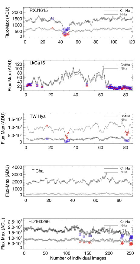
Figure 1: Maximum counts (in ADU) registered in the two filters along the whole exposure for the five targets. The blue squares in the CntHa filter (or red triangles in the NHa one) depict the rejected images in each dataset.

The data reduction was performed using a ZIMPOL customary pipeline developed at ETH Zürich. As a first step, the images were remapped to a square grid of 1024$\times$1024 pix² with a pixel scale of 3$\aas@@fstack{\prime\prime}$6$\times$3$\aas@@fstack{\prime\prime}$6, bias-subtracted, and flat-fielded. Subsequently, the individual images were recentered using a simple Moffat function to estimate the centroid position, as no coronograph was used. This resulted in two individual cubes, one per filter. For the point-spread function (PSF) subtraction, the individual filter datasets (N_Ha and Cnt_Ha) were considered separately to apply a standard angular differential imaging (ADI) processing technique using classical-ADI (cADI), smart-ADI (sADI), and radial-ADI (rADI, see Lafrenière et al., 2007; Chauvin et al., 2012, for a description of these techniques), and (smart) principal component analysis (PCA and sPCA) with one, five, and ten components (Soummer et al., 2012). We note that sPCA is a simple variation of the PCA approach that minimizes the self-subtraction of the signal by rejecting frames too close in time for the eigen-modes calculation. The purpose of using all these algorithms, which handle the speckle noise in different ways, is to secure the detection of point-like sources in the innermost regions of the images.

Simultaneous observations with ZIMPOL ensure that images in two filters present the same speckle pattern. To exploit the spectral diversity of the two filters (Cnt_Ha and N_Ha, inside and outside the H_α line, respectively), we applied a dedicated angular and spectral differential imaging (ASDI) process. The individual Cnt_Ha images were first spatially rescaled to the N_Ha filter resolution, and then flux-normalized considering the total flux ratio between N_Ha and Cnt_Ha within an aperture of $r=10$ pixels. Finally, we performed the subtraction N_Ha-Cnt_Ha frame per frame to exploit the simultaneity of the two observations. ADI processing in cADI, sADI, PCA, and sPCA was then applied to the resulting differential datacube. An example of all the processing algorithms applied to one of the targets (TW Hya) is shown in Figure 9.

Figure 2 shows the final cADI N_Ha, Cnt_Ha and N_Ha-Cnt_Ha (ASDI) images of all the observed targets. We note that all the images have been rotated 134^° counterclockwise to align the camera with the north upwards and east to the left (see Cugno et al., 2019).

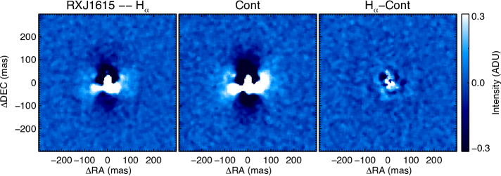
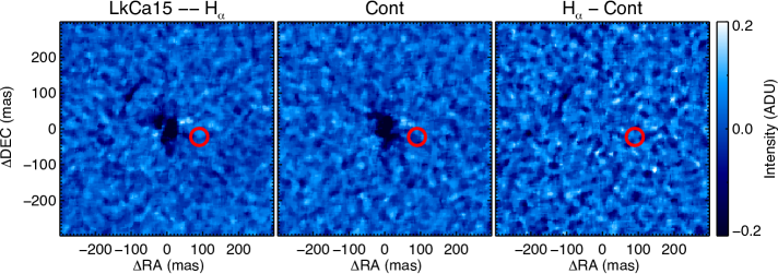
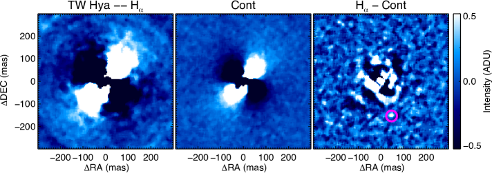
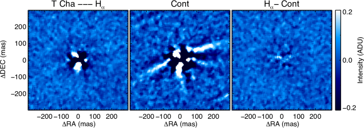
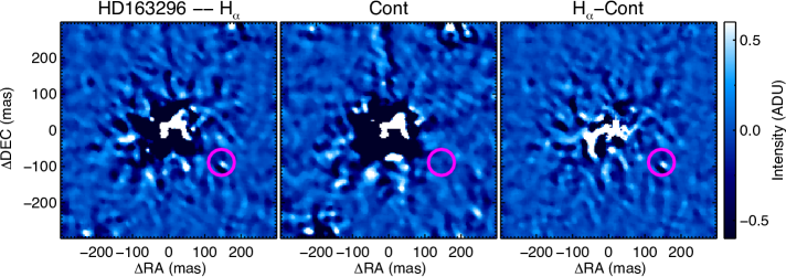
Figure 2: Final cADI images of the five stars observed with SPHERE/ZIMPOL. The panels show the H_α (left) and continuum (middle) images, and their difference (ASDI image, right). All the panels show a FOV of $\sim$ 0.6”$\times$0.6”. In the case of LkCa15, we mark the position of the candidate LkCA15b with a red open circle, while in the case of TW Hya and HD163296 we mark point-like faint detections with magenta circles (see text).

The ADI detection limits in the two filters were estimated from a standard pixel-to-pixel noise map of each filter within a box of 5$\times$5 pixels sliding from the star to the limit of the ZIMPOL field of view. To correct for the flux loss related to the ADI processing, fake planets were regularly injected into the original data cubes before PSF subtraction (every 20 pixels at three different position angles, with a flux corresponding to 100 ADU). The cubes were then reprocessed using the different ADI algorithms, allowing us to estimate the flux loss by computing the azimuthal average of the flux losses for fake planets at the same radii (e.g., Jorquera et al., 2021). The contrast curves at 5$\sigma$ were then obtained using the pixel-to-pixel noise map divided by the ADI flux loss and corrected for small number statistics following the prescription of Mawet et al. (2014) but adapted to our 5$\sigma$ confidence level at small angles with ZIMPOL. The same method was applied for the ASDI dataset to illustrate the gain in speckle subtraction in the inner region below $\sim$100 mas. All the contrast curves are displayed in Figure 3. We note that the Strehl variations along the exposures (that can be of 20%-30% according to Fig. 1) can affect the PSF normalization that we apply to build the contrast curves, which are therefore affected by an error bar of $\sim$ 0.2-0.3 mag. This does not apply to LkCa15, in which the Strehl variations are significantly larger, and therefore this source is expected to show higher uncertainties.

4 Data analysis

As a general result, we do not detect any obvious point-like companion in the analyzed datasets. In the cases of TW Hya and HD163296, we detect some faint point-like emission, the nature of which is discussed in the corresponding subsections below.

Our analysis of the data reveals that, for the cases of TW Hya, T Cha, and RXJ1615, the best contrast in the ADI Cnt_Ha and N_Ha images is obtained for the sADI and sPCA reductions at small separations, while cADI is better at larger separations given the larger number of frames used, minimizing the read-out and background noise. In the case of LkCa15, the faintest object of the sample, cADI provides the best contrast even at small separations, as we are probably entering a low-flux regime for which the temporal evolution of the PSF becomes less critical. For all these objects, the best contrast in the ASDI images is obtained with the cADI reduction: for these images, the SDI technique is very efficient at suppressing temporally variable speckles in the individual N_Ha-Cnt_Ha images, meaning that the subtraction of a median PSF in the final image (cADI reduction) results in a high contrast. Finally, the case of HD 163296 is different, because the small rotation field results in an important self-subtraction in the final images. For this object, we then analyzed the rotated and stacked image without subtracting the PSF, the so-called nADI image. In the following subsections, we discuss the main results for each individual target.

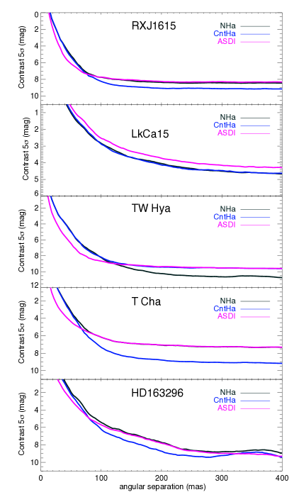
Figure 3: Contrast curves derived from the H_α, continuum, and ASDI (N_Ha - Cnt_Ha) reduced images of the five observed objects.

4.1 RXJ1615

RXJ1615 was observed under good and stable conditions. We only rejected seven individual images, mainly because of a seeing variation during the exposure (changing from 0.6 to 1.0 arcsec, according to the guide probe). The ADI N_Ha and the Cnt_Ha images displayed in Figure 2 show residuals that are not present in the ASDI image, which shows the best contrast at separations below 80 mas.

4.2 LkCa 15

LkCa 15 was observed in December 2018 for $\sim$1.9h, covering a total field rotation of 34 degrees. The average coherence time during the exposure was of $\sim$4 ms. We note that with an R-mag $\sim$12  mag and a declination of $\sim$+24 deg, this is a challenging target for observation with SPHERE/ZIMPOL from the southern hemisphere. The analysis of the maximum counts from the central object reveals very variable conditions, and a significant decrease in the flux in the second part of the exposure with a clear impact on the AO correction quality. Indeed, the individual images show a very variable and elongated PSF. To generate the final images, we selected only those data with the largest number of counts, resulting in a final exposure time of $\sim$1.3 hours and a field rotation of $\sim$25 degrees.

As can be seen in Fig. 2, we do not detect any object in the final images. We improve the contrast curve presented by Cugno et al. (2019) but, given the faintness of the target and the variable conditions, we do not reach sufficient sensitivity to detect the reported companion candidate (Fig. 3). We reach a contrast of $\sim$2.5 mag at the position of LkCa15b reported by Sallum et al. (2015), which is far from the contrast of 5.2 mag achieved with MagAO.

4.3 TW Hya

For TW Hya, the atmospheric conditions were very good and stable, and so we only rejected 7 images (out of 82). The total rotation field is $\sim$108 degrees. The images in the two individual filters show an elongated PSF, and the elongation direction changes with the parallactic angle along the exposure. As a result, the final images show a “butterfly” pattern. This effect, known as a wind-driven halo (WDH), was studied in detail by Cantalloube et al. (2020) and is related to high wind-speeds in the upper layers of the atmosphere. Thanks to the simultaneity of the N_Ha and Cnt_Ha images, this elongated emission is partially suppressed in the ASDI image.

The ASDI image in Fig. 2 shows a faint emission feature located at a separation of $\sim$160 mas SW (magenta circle). We note that this is the only faint emission that is detected in all of the ASDI image regardless of the data processing applied (e.g., cADI, sADI,rADI, PCA or sPCA; see Figure 9 in the Appendix). Inspection of the PSF in the individual N_Ha and CntHa images along the exposure reveals some pinned speckles associated with the spiders that change in flux during the observation. Therefore, it is highly probable that the point-like emission observed in the ASDI images is caused by one of these speckles. Finally, we do not detect any source at the position of the ALMA candidate reported by Tsukagoshi et al. (2019).

4.4 T Cha

T Cha was observed under good and stable conditions, and we did not reject any individual image. The final images do not show any point source, and the contrast in the innermost regions reaches values of 5 mag at 70 mas in the ASDI image. The continuum image shows some radially extended structures. These resemble those detected at IR wavelengths by Pohl et al. (2017), and might be related to the disk itself. We note that this is a difficult object for the detection of accreting protoplanets, given the high disk inclination ($\sim$ 69 degrees, Huélamo et al., 2015).

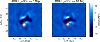
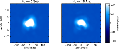
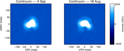
Figure 4: nADI images of HD163296: the nADI reduction includes stacked images after derotation but without subtracting the PSF. The left panels include the reduced data from September 5, while the right panels include data obtained on August 18 for comparison. From top to bottom: ASDI, N_Ha and Cont_Ha final images. The top panels display the position of the star (magenta cross) and the detected point-like emission (red circle) at $\sim$43 au. We display a FOV of 0$\aas@@fstack{\prime\prime}$29$\times$0$\aas@@fstack{\prime\prime}$29.

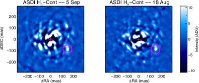
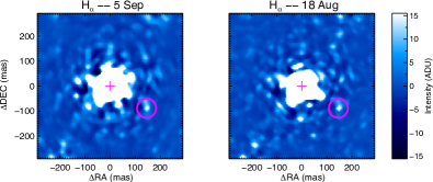
Figure 5: nADI images of HD163296: same as Fig.4, but in this case we display a FOV of 0$\aas@@fstack{\prime\prime}$58$\times$0$\aas@@fstack{\prime\prime}$58, to show the faint detection at $\sim$0$\aas@@fstack{\prime\prime}$17 SW from the central star (magenta circle).

4.5 HD 163296

HD163296 was observed twice: in August and September 2018. In the first dataset, the observing window was not exactly within the specified local sidereal time interval, which is why the target was reobserved later. We note that this is a difficult target for service observations from Paranal Observatory, as it crosses the meridian close to the zenith: the target declination, -21^°57’21”, is close to the observatory latitude, 24^°37’39” S. Hence, we can only obtain data before and/or after the meridian crossing, when the rotation rate is smaller. As a consequence, both datasets show a small rotation field of $\sim$7 and 9 degrees, respectively.

In the first dataset (Aug 2018), the first 130 images were obtained with an individual exposure time (DIT) of 30 seconds, and a large fraction of them were close to (or at) the saturation level, and so we rejected them. The loop then opened, and once it was recovered, a second sequence of 220 unsaturated images with DIT = 20 sec was obtained, but covering only a rotation field of 1.6 degrees. In the second dataset (Sep 2018), we obtained a total of 255 images, each of 20 seconds exposure. In this case, the loop was more stable, and we rejected 12 images out of 255 with the lowest fluxes. We performed our analysis on the second dataset, and the final images are displayed in Figure 2. For completeness, we include an image with a larger field-of-view (FOV) in the Appendix (Figure 10), displaying the position of the planet candidates reported for this source. Without considering the planet candidate proposed by Pinte et al. (2018) at 2.4 arcsec (which is outside the ZIMPOL FOV), we do not detect any clear signal from the planet candidates reported in the literature. On the other hand, we detect a faint emission in the N_Ha and ASDI images at a separation of $\sim$171 mas SW of the central source (magenta circle, Fig. 2). Interestingly, this emission is not observed in the continuum image.

However, we note that a small field rotation can imply important self-subtraction. We therefore also analyzed the derotated images without subtracting the PSF (named “nADI” here). The nADI images are displayed in Figure 4 (FOV of 0.29 $\times$ 0$\aas@@fstack{\prime\prime}$29) and in Fig. 5 (FOV of 0.58 $\times$ 0$\aas@@fstack{\prime\prime}$58). In the former, we can clearly see a bright point-source emission at a separation of $\sim$ 43 mas (4.3 au) in the SE direction (top left panel, red circle). To further investigate the nature of this emission, we also analyzed the nADI unsaturated data obtained in 2018 August 18, and checked that the bright spot appears approximately at the same location. Figure  4 shows that the nADI images in the individual filters show an elongated PSF, which is distorted in the two epochs but in different directions (Fig. 4). Nevertheless, the ASDI images are very similar, displaying an elongated negative pattern in the central regions. For this reason, we think the detected bright spot is probably an artifact connected to the flux variation of a bright Airy ring with the suboptimal AO correction.

Regarding the faint emission reported at 171 mas, it is clearly detected in the nADI images of the two epochs ( Fig. 5). As in the case of the CADI images, it is detected in the ASDI and N_Ha images, but not in the continuum, as expected for an accreting protoplanet. The emission is located at 171 mas and PA$\sim$239 degrees. We note that this emission is not reported in Xie et al. (2020), given that the MUSE data show strong residuals at separations $<$0$\aas@@fstack{\prime\prime}$5. According to Isella et al. (2018), the possible candidate would be placed after the bright ring at 14 au (named B14). The nature of this source (real detection or speckle) is uncertain, and would require further observations with a better rotation field coverage. Finally, we note that despite the small field rotation, the cADI is achieving very similar performances to nADI down to 50-80 mas.

5 Results

5.1 H_α emission from potential protoplanet companions

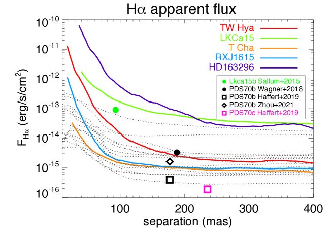
Figure 6: Apparent H_α line fluxes for the five observed targets as a function of distance, in mas, from the central star. Gray dotted lines show the fluxes of the sample observed by Zurlo et al. (2020) also with SPHERE/ZIMPOL.

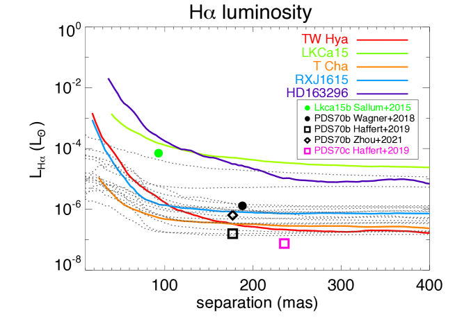
Figure 7: H_α line luminosities for the five observed targets. The gray dotted lines represent the H_α line luminosities from the sample studied by Zurlo et al. (2020)

The high sensitivity of the ZIMPOL images allowed us to derive N_Ha contrast curves with $\Delta\,mag$ between of $\sim$6 and 8 at $\sim$100 mas from the central sources (except in the case of LkCa15). We can use these curves to derive upper limits to the H_α line emission of potential protoplanet companions. To this aim, we first estimated the pure H_α line flux (continuum subtracted) of the primary stars, following the methodology explained in Cugno et al. (2019). We first performed aperture photometry for the primaries in the ContHa and N_Ha filters using an aperture radius of 1.5 arcsec in all the images of the stacked cube, deriving the mean count rate ($cts$), and its uncertainty, $\sigma$/$\sqrt{n}$, with $\sigma$ being the standard deviation, and $n$ the number of images. We then estimated the flux in the Cnt_Ha and N_Ha filters following the expression:

$$F_{filter}=cts_{filter}\times 10^{0.4(airm*k_{\lambda}+m_{mode})}\times c_{zp}^{filter},$$ (1)

where $cts$ is the measured count rate (cts/s), $airm$ the average airmass (see Table 2), $k_{\lambda}$ the atmospheric extinction at Paranal (0.085 and 0.082 for Cnt_Ha and N_Ha, respectively, Patat et al., 2011), $m_{mode}$ (with a value of –0.23 mag) a factor taking into account the enhanced transmission of the used R-band dichroic with respect to the gray beam splitter, and $c_{ZP}^{filter}$ is the zero point of the corresponding filter. As we have observed with the Cnt_Ha in the FW1 and N_Ha in the FW2, the corresponding zero points are 1.59$\pm$0.05 $\times$ 10^-17 erg/(cm² $\cdot\AA\cdot$ count) and 9.2${}^{+4}_{-0.5}$ $\times$ 10^-16 erg/(cm² $\cdot$ count), respectively (Schmid et al., 2017). The estimated flux uncertainties account for the errors in the count rates and the zero points.

Once the Cnt_Ha and N_Ha fluxes are estimated, we can derive the count rate due to the continuum emission in the line filter (N_Ha), following Eq. (2) in Cugno et al. (2019). If we subtract the derived count rate from the one measured in the line filter, we can estimate the pure H_α emission in the N_Ha filter for each central star (named $F_{H_{\alpha}}$). The derived fluxes in the two ZIMPOL filters are provided in Table 3 together with the pure H_α stellar emission in N_Ha.

We corrected the stellar H_α line fluxes ($F_{H_{\alpha}}$) for interstellar extinction estimating $A_{R}$ from $A_{V}$ (included in Table 1), applying the extinction law from Rieke & Lebofsky (1985). We then used the dereddened fluxes to estimate the line luminosities ($L_{H\alpha}$) of the stars using the distance included in Table 1. For completeness, we also derived the accretion properties of the central stars following the procedure described in Appendix C, where we also briefly discuss the obtained values.

Table 3: Continuum and H_α line fluxes estimated for the primary stars and derived accretion parameters

Target	$F_{\rm Cnt\_Ha}$	$F_{\rm N\_Ha}$	$F_{\rm H\alpha}$	$L_{\rm H\alpha}$∗	$L_{\rm acc}$	$M_{\rm acc}$
	(10-12 erg/s/cm2)	( 10-12 erg/s/cm2)	( 10-12 erg/s/cm2)	(10-3 L⊙)	(L⊙)	(M⊙/yr)
RXJ1615	2.70$\pm$0.09	2.1$\pm$0.9	1.5$\pm$0.7	1.7$\pm$0.5	0.042	5.5$\times$10-9
LkCa 15	1.16$\pm$0.04	1.8$\pm$0.8	1.5$\pm$0.7	1.8$\pm$0.5	0.043	2.1$\times$10-9
TW Hya	5.4$\pm$0.2	29.9$\pm$13.0	28.7$\pm$12.5	3.3$\pm$1.4	0.085	5.1$\times$10-9
T Cha	8.3$\pm$0.2	2.1$\pm$0.9	0.3$\pm$0.1	0.23$\pm$0.03	0.004	2.0$\times$10-10
HD 163296	155$\pm$4	116$\pm$50	82$\pm$36	26.3$\pm$11.5	3.235	9.8$\times$10-8

^∗ Dereddened values

We used the dereddened H_α fluxes together with the contrast curves in the N_Ha filter to derive the $H_{\alpha}$ line fluxes and luminosities at different separations from the stars. We note that we used the contrast curves obtained from the cADI reduction for all the targets. In the case of TW Hya, T Cha, and RXJ1615, this could be considered a conservative approach for the innermost regions, but this is not critical. The flux detection limits and luminosity upper limits are shown in Figures 6 and 7, respectively. For comparison, we include the curves obtained for the sample of objects observed by Zurlo et al. (2020) with SPHERE/ZIMPOL. As shown in Fig. 7, for three objects (T Cha, TW Hya, and RXJ1615), we obtained H_α line luminosities of $\sim$0.5–1$\times 10^{-6}\,L_{\odot}$ at separations of 200 mas, which is comparable to the values derived by Zurlo et al. (2020) for most of their sources. In the case of HD 163296 and LkCa15, the estimated line luminosities are $\sim$3$\times 10^{-5}\,L_{\odot}$ and $\sim$1$\times 10^{-4}\,L_{\odot}$ at 200 mas, respectively. Also, for the sake of comparison, we include the H_α fluxes of PDS70 b and c, and LkCa15 b in Fig. 6.

For each target, we estimated contrasts, H_α line fluxes, and luminosities at the projected separations where the innermost dust gaps (corresponding to the disk semi-major axis) or planet candidates have been detected (see Table 4). We note that these are rough estimations, because we have not corrected the curves by the disk inclinations. The results are included in Table 4. For the dust disk gaps (marked with a “g’’), and whenever available, we have included the planet mass that could be responsible to carve it. For the planet candidates detected in IR imaging or submm ALMA data (marked with a “p’’), we have included the planet mass estimated from the corresponding observations. As seen in Table 4, for the targets with good-quality data, we reach upper limits to the H_α line luminosity of 10^-6 L_⊙ in the innermost gaps, and $\sim$10^-7 L_⊙ in the outermost ones. For LkCa 15 and HD 163296, these upper limits are between 10^-4 L_⊙ and 10^-6 L_⊙, respectively.

Table 4: 5-$\sigma$ upper limits to the N_Ha contrast, dereddened H_α line fluxes and luminosities, and accretion luminosities at the projected separations of dust gaps (corresponding to the disk semi-major axis), and planet candidate detections.

Target	Projected Separation		Planet mass	N_Ha contrast	$F_{\rm H\alpha}$	$L_{\rm H\alpha}$	$logL_{\rm acc}$†
	(arcsec)	(au)∗	(MJup)	(mag)	(10-15 erg/s/cm2)	(10-6 L⊙)	(L⊙)
RXJ1615	0.141,(g)	22	4.51	8.1	$<$ 1.3	$<$ 0.98	$<$ -4.1
	0.502,(g)	78	0.23	8.6	$<$ 0.8	$<$ 0.64	$<$ -4.3
LkCa 15	0.0934,(p)	15	65	2.7	$<$ 190	$<$ 150	$<$-2.0
	0.276,(g)	43	0.53	4.4	$<$ 38	$<$ 0.29	$<$ -2.7
TW Hya	0.107,(g)	6	0.041	8.2	$<$ 14	$<$ 1.6	$<$ -3.9
	0.377,(g)	22	0.153	10.6	$<$ 1.7	$<$ 0.19	$<$ -4.8
	0.878,(p)	52	0.058	11.1	$<$ 1.0	$<$0.11	$<$ -5.0
T Cha	0.0939,(g)	9	1.29	6.0	$<$ 1.6	$<$ 0.52	$<$ -4.4
HD 163296	0.1010,(g)	10		5.4	$<$ 700	$<$ 220	$<$ -1.9
	0.4411,(g)	45		9.5	$<$ 16	$<$ 5.2	$<$ -3.4
	0.512,(p)	51	612	9.9	$<$ 10	$<$ 3.3	$<$ -3.6
	0.6713,(p)	68	113	10.6	$<$ 5.6	$<$ 1.8	$<$ -3.8
	0.7714,(p)	78	114	10.8	$<$ 4.5	$<$ 1.4	$<$ -3.9

^∗ Estimated assuming Gaia EDR3 distances from Table 1; ^† Estimated using the prescription of Aoyama et al. (2021) (see text). ^(g): Disk gaps; ^(p): Planet candidates;

¹ Asensio-Torres et al. (2021); ² de Boer et al. (2016); ³ Dong & Fung (2017), values for a viscosity parameter $\alpha$ 10^-3; ⁴ Sallum et al. (2015); ⁵ Kraus & Ireland (2012); ⁶ Thalmann et al. (2016); ⁷ van Boekel et al. (2017); ⁸ Tsukagoshi et al. (2019); ⁹ Hendler et al. (2018), position of the gap minimum; ¹⁰Isella et al. (2018); ¹¹ Isella et al. (2016); ¹² Guidi et al. (2018); ¹³ Pinte et al. (2020); ¹⁴ Izquierdo et al. (2021)

5.2 Accretion luminosity of potential planet companions

The accretion luminosity ($L_{\rm acc}$) of young planets is an important parameter as it be used to estimate their accretion rate, and therefore to understand how planets grow as they evolve. The $L_{\rm acc}$ of planet candidates can be estimated from the observed $H_{\alpha}$ line emission, after assuming a model to explain the physical conditions to form the line. To illustrate the impact of the different models on the $L_{\rm acc}$ estimations, we compared three different approaches, and applied them to the sources observed with SPHERE/ZIMPOL.

Previous works (e.g., Close et al., 2014; Sallum et al., 2015; Cugno et al., 2019) calculated the accretion luminosity of young giant planets assuming that it scales with $L_{\rm H_{\alpha}}$ as in low-mass Classical T Tauri stars (CTTSs). They therefore applied the relation derived by Rigliaco et al. (2012):

$$\log(L_{\rm acc}/L_{\odot})=(2.99\pm 0.16)+(1.49\pm 0.05)\times\log(L_{\rm H\alpha}/L_{\odot}).$$ (2)

However, as already mentioned in different works, this relation is not necessarily valid for young planets, because CTTSs show different properties (see e.g., Zhou et al., 2014; Thanathibodee et al., 2019), and the accretion process can take place through a different mechanism. We include this approach here so that our results can be compared with previous works, but it is important to estimate $L_{\rm acc}$ using appropriate models developed for young planets, and not for young stars.

In this context, Aoyama et al. (2018) developed a 1D model of shock-heated gas for planetary masses, and studied the hydrogen line emission from young giant planets. In their model, the $H_{\alpha}$ line emission is generated in the post-shock gas located either in the CPD or on the planet surface (Aoyama & Ikoma, 2019). In an extension of this work, and using a broad range of planetary masses and accretion rates, Aoyama et al. (2021) provided a $L_{H_{\alpha}}-L_{\rm acc}$ relationship (Eq. 3) assuming a magnetospheric accretion model and considering that the accretion shock is located on the planetary surface:

$$\log(L_{\rm acc}/L_{\odot})=1.61+0.95\times\log(L_{\rm H\alpha}/L_{\odot}),$$ (3)

for $L_{\rm acc}\leq 10^{-4}L_{\odot}$ , although, as explained by the authors, higher values barely affect the fit. The half-spread at a given $L_{H_{\alpha}}$ is of 0.3 dex.

A different model was presented by Szulágyi & Ercolano (2020, SE2020 hereafter), in which planets grow through boundary layer accretion (see e.g., Owen & Menou, 2016) in which the material is accreted directly onto the planet and its CPD from the circumstellar disk. SE2020 computed hydrogen recombination line emission from 3D thermo-hydrodynamical models of forming planets with masses of 1-10 M_Jup, incorporating extinction, line variability, and excluding magnetic fields. In their 3D simulations, all the line luminosity comes from the accretion shock on the surface of the CPD. SE2020 provided parametric equations between the accretion luminosity and the H_α line emission for different size distributions and chemical compositions of the circumstellar dust grains. For our comparison, we considered two different opacity cases included in their model: a disk with a dust mixture of silicates, water ice, and carbon (the most realistic case in terms of composition), and a gas-only disk, that is, a dust-depleted disk to consider the largest disk gaps where planets can grow, and which are almost devoid of dust. We note that the latter is an extreme scenario and will only provide upper limits to the line luminosities. SE2020 derived the following relationships for these two opacity cases:

$$\log(L_{\rm acc}/L_{\odot})=0.028\times\log(L_{H_{\alpha}}/L_{\odot})-2.55$$ (4)

for the disk with a mixture of silicates, water ice, and carbon, and

$$\log(L_{\rm acc}/L_{\odot})=0.32\times\log(L_{H_{\alpha}}/L_{\odot})-2.18$$ (5)

for the gas-only case.

In order to translate our $L_{H_{\alpha}}$ observational limits into accretion luminosities, we estimated $L_{\rm acc}$ considering all the models described above, and the 5-$\sigma$ $H_{\alpha}$ luminosity curves of the objects included in this work and in Zurlo et al. (2020). The results are represented in Figure 8, where we highlight the results obtained for RXJ1615 (average case) to see the differences between the models more clearly.

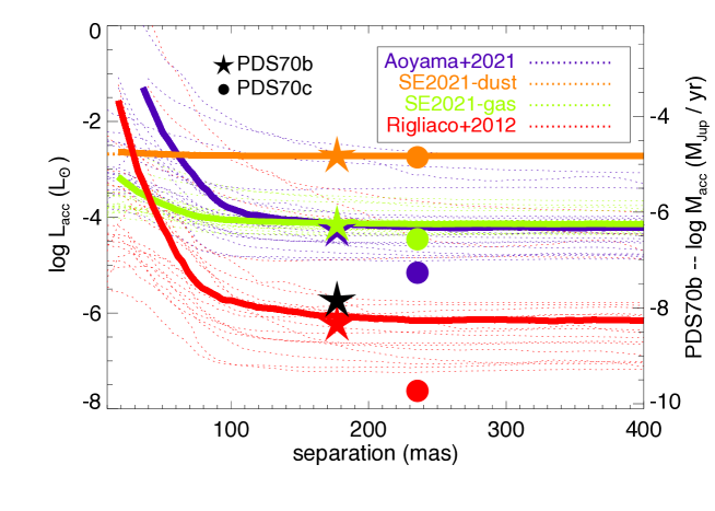
Figure 8: Accretion luminosities estimated from the $L_{\rm H_{\alpha}}$ contrast curves, and using four different relations given in Eqs. 2 – 5 (see text). These four relationships are represented with different colors as described in the upper right panel of the figure. The dotted lines correspond to all the individual objects observed in this work and in Zurlo et al. (2020), while the thick solid lines represent the results for RXJ1615 (as an average case) to highlight the difference between the four models. We represent the estimated $L_{\rm acc}$ values for planets PDS70b (starred symbols) and PDS70c (filled circles) using the four models. For completeness, we include the $L_{\rm acc}$ value of PDS70b estimated by Zhou et al. (2021) using a slab model (black star). The corresponding $M_{\rm acc}$ values for planet PDS70b, assuming a planet mass of 1 M_Jup and a planet radius of 1.75 R_Jup, are displayed on the right y-axis.

As seen in Fig. 8, for a given $L_{H_{\alpha}}$, the planetary models predict accretion luminosities higher than those previously calculated using stellar relations. If we considered a separation of for example 200 mas, the estimated accretion luminosity is on average two orders of magnitude higher (or almost three times in the case of the dusty disk from SE2020) than the $L_{\rm acc}$ derived with the relation of Rigliaco et al. (2012). Therefore, when using planetary models, an observed $L_{H_{\alpha}}$ would correspond to a higher $M_{\rm acc}$ than previously estimated for a given planet mass and radius. As explained by Aoyama et al. (2021), this could indicate that only the strongest accretors can produce an H_α emission line bright enough to be detected, and could explain the lack of detections of the different surveys.

To illustrate the impact of using different models, we estimated the $L_{\rm acc}$ of the confirmed protoplanets PDS70bc using the four approximations described above. In the case of PDS70b, we consider a line luminosity of $L_{H_{\alpha}}=6.5\times 10^{-7}\,L_{\odot}$ (Zhou et al., 2021), while in the case of PDS70c we use the line flux obtained by Haffert et al. (2019). The results are included in Fig. 8. For completeness, we also include the $L_{\rm acc}$ value of PDS70 b derived by Zhou et al. (2021), who fit UV and H_α observations with a slab model. Clearly, the different models can provide $L_{\rm acc}$ that can differ by more than three orders of magnitude, which translates to a very different accretion rate. For example, in the case of PDS70b, considering a mass of 1 M_Jup and a radius of 1.75 R_Jup (Stolker et al., 2020), we can estimate the accretion rate following Gullbring et al. (1998), and assuming $R_{\rm in}$ = 5 $R_{p}$ as in (Zhou et al., 2021). The derived values are displayed on the right y-axis of Figure 8. This graph illustrates that, depending on the model used, the derived accretion rates range between $\sim$ 1$\times$10^-8 and 1$\times$10^-5 M_Jup/yr, meaning that the protoplanet can be classified as either a strong or faint accretor.

Finally, and for completeness, we estimated the $L_{\rm acc}$ from the $L_{H_{\alpha}}$ for the planet candidates and gaps detected around the five sources studied in this work. For this estimation, we used the prescription of Aoyama et al. (2021) (Eq. 3). The values are included in the last column of Table 4, and range between $\log(L_{\rm acc})\sim-2.0$ and $-5.0\,L_{\odot}$ for the different sources and separations.

6 Discussion

Cugno et al. (2019) and Zurlo et al. (2020) carried out ZIMPOL/H_α surveys to detect accreting protoplanets in the gaps of transitional disks. Adding up the new targets observed in this study, there are a total of 18 objects observed with ZIMPOL: 8 T Tauri stars and 10 Herbig Ae/Be and F-type stars. Although most of these ZIMPOL observations were obtained under good conditions, reaching a very high contrast, no accreting protoplanets were detected. The only companion detected with ZIMPOL was around the source HD 142527, confirming its previous H_α detection (Close et al., 2014).

Other works using different instrumentation have reported similar results: Xie et al. (2020) did not detect any new accreting protoplanet around five young stars using MUSE on the VLT, even though this instrument can reach fainter detection limits in the H_α line apparent flux (a factor of $\sim$5 fainter) in comparison to SPHERE/ZIMPOL. Finally, Uyama et al. (2020) observed five T Tauri stars with Subaru/SCExAO+VAMPIRES, reporting the nondetection of nearby planet companions.

We should note that most of these surveys reach the highest contrast at separations of larger than $\sim$ 100-150 mas, which translates to projected separations of larger than 10-15 au for nearby objects. The deprojected separations can be even larger, which means that we obtained the best sensitivity in regions where giant planets are difficult to form. On the other hand, the only protoplanets confirmed so far are detected at large projected separations from the central star: 0$\aas@@fstack{\prime\prime}$195 (22 au) and 0$\aas@@fstack{\prime\prime}$22 (30 au) for PDS70 b and c, respectively (Keppler et al., 2018; Mesa et al., 2019b). Despite the fact that the ZIMPOL observations from different surveys provide very good contrast at similar separations for some of the observed targets, no protoplanets were detected in the same spatial range.

Apart from the lack of sensitivity at very small separations, the lack of H_α detections could be explained by a combination of other factors; for example, weak and/or episodic accretion, circumstellar and circumplanetary disk extinction, and/or the presence of planets with insufficient mass to produce a detectable H_α line emission.

As explained in the previous section, a large number of works estimating accretion luminosities and accretion rates in protoplanets used relations derived for TTSs, which are not valid in the planetary regime. When using planetary models, the result is that only the strongest accretors could be detected in the $H_{\alpha}$ line, and this could explain why previous surveys reported a large number of nondetections. We compared this result with the predictions from planet population synthesis performed by Mordasini et al. (2017). In the “cold accretion” scenario described by these latter authors, the accretion luminosity caused by shocks is radiated away from the planet, meaning that they can derive the accretion luminosities as a function of planet mass for the planet population at 3 Myr (their Figure 7, cold-nominal case). According to the results from planetary models, current H_α observations would only be sensitive to either planets more massive than 1 M_Jup with accretion luminosities higher than 10^-4 $L_{\odot}$, or to the most massive planets with M_p $>$ 10 M_Jup (a very reduced sample), assuming the dust model (SE2021-dust) by Szulágyi & Ercolano (2020). In this context, PDS 70 b might fit with the scenario described by Mordasini et al. (2017) as a limiting case, given its mass (1.0$\pm$0.5 $M_{\rm Jup}$) and the estimated accretion luminosity when planetary models are considered (see Figure 8). In the case of planet PDS70 c, with an estimated mass of lower than 5 M_Jup (Mesa et al., 2019b), it could fit in this scenario only if $L_{\rm acc}$ is estimated using the models by Szulágyi & Ercolano (2020).

Regarding the episodic accretion, there is only one study that has monitored the H_α line emission in the protoplanet PDS70 b: Zhou et al. (2021) observed the planet in six epochs over a five-month timescale with the HST, and their high-quality data did not support a H_α line variability at a level higher than 30%. In the same respect, it would be extremely useful to perform a dedicated campaign to study the long-term variability of the H_α line emission of the two confirmed protoplanets PDS70 b and c.

Another parameter that can affect the measured $H_{\alpha}$ luminosity is the mass of the accreting planets. As explained in SE2020, there is a trend between planet mass and line luminosity, as the temperature is higher in the vicinity of a more massive planet (resulting in a higher hydrogen ionization), and the extinction decreases because the gap opened is larger (see below). As a result, these models predict that when considering the most realistic disk opacities, only giant planets with masses above 10 M_Jup show a clearly detectable H_α emission line at the level of $L_{H_{\alpha}}\sim 10^{-2}L_{\odot}$. When taking into account line variability due to extinction and/or episodic accretion, SE2020 show that 5 M_Jup planets can be detected with $L_{H_{\alpha}}\sim 10^{-8}-10^{-5}L_{\odot}$, some of these values being within the ZIMPOL detection limits. We note that in the present work, we did not consider the extinction due to the dust in the circumstellar disks and/or the CPD when estimating $L_{H_{\alpha}}$.

In the case of transitional disks, Sanchis et al. (2020) studied the effect of circumstellar extinction on giant planets, and concluded that it varies depending on the mass of the object because this parameter defines the width and depth of the opened gaps. According to their estimations, planets with masses of 1-2 $M_{\rm Jup}$ would show very high extinction, while planets with 5 M_Jup or higher, would show a negligible extinction. In our sample of five stars, the predicted planet masses range between $\sim$ 16 M_Earth and 6 M_Jup (see Table 4). Excluding LkCa15 b because of the controversy surrounding its existence, the most massive protoplanet candidate is that of 6 $M_{\rm Jup}$ around HD163296 proposed by Guidi et al. (2018) based on IR observations. We did not detect any source at the position of this candidate, although we are limited by the small rotation field (although the nADI images do not reveal any source). Another interesting source is RXJ1615, with a predicted 4.5 M_Jup planet at 22 au according to Asensio-Torres et al. (2021). However, and regardless of the good contrast, we do not detect any accreting source at the given separation.

Even in the case of large gaps in the circumstellar disks, we still have to consider the extinction related to the CPDs, given that the H_α flux could be more or less absorbed depending on the CPD inclination with respect to the observer. We do not know a priori the CPD inclinations, but if these are similar to those of primary disks, we should have been able to detect some protoplanets, because a large fraction of the stars observed in the different surveys are surrounded by disks with both low and intermediate disk inclinations. The protoplanets PDS70 bc, which are surrounded by CPDs (see Christiaens et al., 2019; Benisty et al., 2021), were detected inside the gap of a disk with an inclination of $\sim$52 degrees (Keppler et al., 2018). In this context, the case of T Cha is the most challenging given that the disk inclination is 67 degrees. We can therefore conclude that the combination of some/all of the factors explained above could explain the lack of detections of accreting planets around the explored objects.

Finally, we note that all of the surveys and works focusing on the search of accreting protoplanets through H_α observations have studied stars in the Class II stage. However, there is already observational evidence of disks around Class I protostars displaying similar substructures (e.g., rings, gaps, cavities) to those observed in Class II objects (e.g., Segura-Cox et al., 2020; Sheehan et al., 2020). In addition, evidence of grain growth, a key element to planet formation, has been suggested in at least one Class I object (Harsono et al., 2018). Another possible scenario to explain the lack of H_α detections would therefore be that planet formation takes place earlier than predicted by models, meaning that the bulk of the accretion luminosity during the planet formation process occurs sooner in their evolution when stars are still embedded in their parental clouds. However, further investigations should clarify whether Class I disk substructures are indeed caused by planets or are the result of other processes (e.g., magneto-rotational instabilities, snowlines). Nevertheless, any scenario would still have to explain the detection of protoplanets PDS70 b and c around a relatively old star.

7 Conclusions

We present high-angular-resolution $H_{\alpha}$ observations of five disks with signatures of planet formation. As found in previous works using SPHERE/ZIMPOL, we do not report any clear detection of accreting planets regardless of the good instrumental performance. We only report a very faint H_α point-like emission around TW Hya, a probable speckle related with a spike, and HD163296 based on emission detected in the ADI N_Ha and ASDI images, but additional observations are required to confirm its true nature. The lack of detections could be explained by different factors such as low contrast at smaller separations ($<$150 mas) where giant planets are more likely to form, a majority of low-mass, low-accreting planets, circumplanetary extinction, and/or episodic accretion.

The accretion luminosities derived from the upper limits to the H_α luminosities vary significantly when using relations from different planetary models and, in general, they are all higher than the ones derived using stellar relations from CTTs.

Future observations with other facilities such as the James Webb Space Telescope, or with ground-based telescopes with more advanced AO systems, such as MagAO+ (see Close, 2020) or SPHERE+, will help us to access more targets and to study different accretion tracers (e.g., $H_{\alpha}$, Pa $\beta$ or/and Br $\gamma$ lines), allowing us to increase the detection of accreting protoplanets in the gaps of transitional disks. Dedicated monitoring campaigns of detected protoplanets in these tracers will also help us to understand their short- and long-term variability, and to study episodic accretion in more detail.

Appendix A TW Hya: comparison of final images from different processing algorithms

This Appendix shows the result of applying the different processing algorithms explained in section 4 to the case of the star TW Hya. This object is of particular interest because of the detection of faint point-like emission at a separation of $\sim$160 mas (9.1 au) from the central source. The results are displayed in Figure 9. The upper panels correspond to the ASDI images, while the middle and lower panels represent the ADI N_Ha and CntHa images.

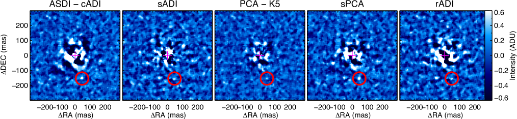
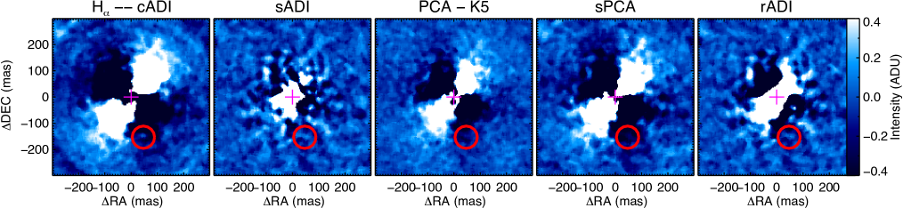
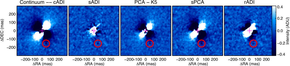
Figure 9: ASDI (top) and ADI N_Ha (middle) and CntHa (bottom) images of TW Hya using different processing techniques. In the case of PCA processing, we show the results obtained when considering five components (denoted with K5). The bright spot detected at $\sim$160 mas SW is encircled in all the images.

Appendix B HD163296: position of the published planet candidates

Figure 10 includes the ZIMPOL images of HD163296, where we represent the position of the planet candidates reported for this source in previous works.

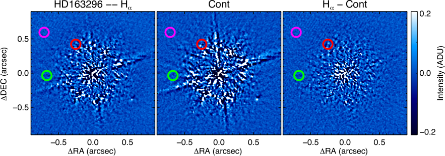
Figure 10: ADI N_Ha (left), ADI CntHa (middle) and ASDI (right) images of HD163296 displaying a FOV of 0$\aas@@fstack{\prime\prime}$9 $\times$ 0$\aas@@fstack{\prime\prime}$9. The planet candidates reported by Guidi et al. (2018), Pinte et al. (2020), and Izquierdo et al. (2021) are represented by red, green, and magenta circles, respectively. We note that the planet candidate reported by Pinte et al. (2018) at 2$\aas@@fstack{\prime\prime}$4 is outside the ZIMPOL FOV.

Appendix C Accretion rates of the primary stars

In Section 5 we estimate the H_α line fluxes of the primary stars in the sample. We compare the derived values with those previously obtained in different works and we also estimate their accretion luminosities and accretion rates.

For the T Tauri stars in the sample, we estimated the accretion luminosity ($L_{\rm acc}$) following the relationship derived by Alcalá et al. (2017):

$$\log(L_{\rm acc}/L_{\odot})=(1.74\pm 0.09)+(1.13\pm 0.07)\times\log(L_{\rm H\alpha}/L_{\odot}).$$ (6)

We then estimated the accretion rate ($M_{\rm acc}$) of all the objects using the expression from Gullbring et al. (1998):

$$M_{\rm acc}=1.25\times\frac{L_{\rm acc}R_{*}}{GM_{*}},$$ (7)

where $M_{*}$ and $R_{*}$ are the stellar mass and radius (included in Table 1), respectively. The expression assumes a disk truncation radius of 5 $R_{\odot}$.

In the case of HD163296, we estimated both $L_{\rm acc}$ and $M_{\rm acc}$ using the relations derived by Fairlamb et al. (2017) for Herbig Ae/Be stars:

$$\log(L_{\rm acc}/L_{\odot})=(2.09\pm 0.06)+(1.00\pm 0.05)\times\log(L_{H\alpha}/L_{\odot}),$$ (8)

and

$$M_{\rm acc}=\frac{L_{acc}\,R_{*}}{G\,M_{*}}$$ (9)

We include the derived $L_{\rm acc}$ and $M_{acc}$ (expressed in $M_{\odot}$/yr) in Table 3. We briefly discuss the results obtained for the individual objects below:

RXJ1615: The estimated H_α line flux for this T Tauri star is 1.5$\pm$0.7 $\times 10^{-12}$ erg/s/cm². Using the stellar values included in Table 1, we estimated an accretion rate of 9.8$\times$10^-9 M_⊙/yr. The line flux is consistent with the value derived by Manara et al. (2014), 2.24$\pm$0.05 $\times 10^{-12}$ erg/s/cm², within the uncertainties.

For this particular object, and to test our photometric calibration, we performed high-resolution spectroscopy of RXJ1615 with the Magellan Echellette Spectrograph (MagE) mounted on the 6.5m Baade telescope in Las Campanas Observatory 10 days after the ZIMPOL observations. We obtained two spectra of 60 seconds each with the 5 arcsec slit on April 30 2018 —10 days after the ZIMPOL data was obtained— under photometric conditions. The target was observed at airmass 1.02. A spectrophotometric standard star was observed immediately after RXJ1615 at airmass 1.07, and with the same slit.

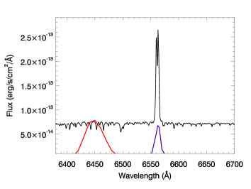
Figure 11: MagE spectrum of RXJ1615. We display the wavelength range containing the H_α emission line. The red and blue lines represent the transmission curves of the ZIMPOL Cnt_Ha and N_Ha filters, respectively.

The spectra were reduced with a dedicated pipeline. The processing includes bias subtraction and flat-field correction. We used thorium-argon (ThAr) exposures obtained after the science spectrum to wavelength-calibrate the data. We then flux-calibrated the science spectrum using the standard star. We used the spectrum to perform synthetic photometry, deriving an R-band magnitude of 11 mag, close to the tabulated value of 11.2 mag (e.g., Makarov 2007).

Figure 11 shows part of the calibrated spectrum containing the H_α line, together with the ZIMPOL Cnt_Ha and N_Ha transmission curves. We measure a H_α line flux of 1.2$\pm$0.2 $\times$ 10^-12 erg/s/cm², and a continuum flux density of 7.2$\times$ 10^-14 erg/s/cm²/Å. The two values are consistent with the derived ZIMPOL data, validating the H_α line flux estimation procedure.

LkCa 15: This object was spectroscopically studied in detail by Whelan et al. (2015) using VLT/XSHOOTER data. The star was observed in six epochs displaying clear H_α variability. The H_α line flux measured in the different epochs varied between (0.7 – 1.56)$\times 10^{-12}$ erg/s/cm². The derived H_α ZIMPOL flux lies within this interval, being very close to the strongest value. On the other hand, Manara et al. (2014) reported a factor $\sim$2 stronger H_α line flux of 3.1$\pm$0.1$\times 10^{-12}$ erg/s/cm².

The estimated ZIMPOL accretion rate is $M_{\rm acc}\sim 2\times 10^{-9}$ $M_{\odot}$/yr. However, if we consider the minimum and maximum line fluxes measured in the works mentioned above, and the stellar parameters from Table 1, we derive accretion rates of $\sim 9\times 10^{-10}-4.8\times 10^{-9}\,M_{\odot}$/yr.

TW Hya: The H_α line flux and profile of this target is very variable with rapid changes in timescales of days (see e.g., Dupree et al. 2012). The H_α line flux derived in the ZIMPOL observations (2.87$\pm$1.25$\times 10^{-11}$ erg/s/cm^-2) is consistent within the uncertainties with the value reported by Manara et al. (2014): 2.39$\pm$0.04$\times 10^{-11}$ erg/s/cm^-2. Using the stellar parameters included in Table 1, we estimate an accretion rate of $M_{\rm acc}\sim 5\times 10^{-9}M_{\odot}$/yr.

T Cha: This object is known to be extremely variable both in the optical continuum and the H_α line (see e.g., Alcala et al. 1993; Schisano et al. 2009; Cahill et al. 2019). In fact, the line has been observed both in emission and in absorption. Previous works suggested that the variability could be related with strong circumstellar extinction due to the presence of dusty clumps in the inner disk.

We estimate a very low H_α emission flux in the ZIMPOL data, resulting in an accretion rate of $M_{\rm acc}\sim 2\times 10^{-10}\,M_{\rm\odot}$/yr. This value is between the rate reported by Schisano et al. (2009), estimated through the relationship between $M_{\rm acc}$ and the 10% width of the H_α line (4$\times 10^{-9}\,M_{\rm\odot}$/yr), and the value estimated by Cahill et al. (2019) using the H_α line in emission observed in one of their analyzed spectra (8$\times 10^{-11}$ $M_{\odot}$/yr).

We note that we estimated a continuum flux density of $\sim$ 2$\times 10^{-13}$ erg/s/cm²/Å  in the ZIMPOL data, which is comparable to the value derived by Cahill et al. (2019) for an extinction value of 1.2 mag. Hence, we adopted this value for $A_{v}$.

HD163296: The H_α emission of this object has been studied by different authors: Wichittanakom et al. (2020) reported a H_α line flux of 1.35$\pm$0.05$\times$10^-10 erg/s/cm^-2, while Fairlamb et al. (2015) estimated a line flux of 1.06$\pm$0.09 $\times$ 10^-10 erg/s/cm^-2. Mendigutía et al. (2013) studied data for HD163296 from five epochs obtained on timescales from days to months. We converted their provided maximum and minimum H_α luminosities into fluxes using their assumed distance of 130 pc, obtaining line fluxes of 1.5 – 2.0 $\times$ 10^-10 erg/s/cm^-2.

Using the ZIMPOL data, we report a H_α line flux of 0.82$\pm$0.36$\times$10^-10 erg/s/cm^-2, which is within the reported values in previous works within the uncertainties. Using equations 8 and 9, we estimate an accretion rate of 9.8$\times$10^-8 M_⊙/yr. If we consider the minimum and maximum H_α line fluxes estimated for the object, and the updated stellar parameters included in Table 1, the accretion rate can vary between 0.9 and 2.4 $\times$ 10^-7 M_⊙/yr.