Improving Visual-Semantic Embedding with Adaptive Pooling and Optimization Objective

Abstract

Visual-Semantic Embedding (VSE) aims to learn an embedding space where related visual and semantic instances are close to each other. Recent VSE models tend to design complex structures to pool visual and semantic features into fixed-length vectors and use hard triplet loss for optimization. However, we find that: (1) combining simple pooling methods is no worse than these sophisticated methods; and (2) only considering the most difficult-to-distinguish negative sample leads to slow convergence and poor Recall@K improvement. To this end, we propose an adaptive pooling strategy that allows the model to learn how to aggregate features through a combination of simple pooling methods. We also introduce a strategy to dynamically select a group of negative samples to make the optimization converge faster and perform better. Experimental results on Flickr30K and MS-COCO demonstrate that a standard VSE using our pooling and optimization strategies outperforms current state-of-the-art systems (at least 1.0% on the metrics of recall) in image-to-text and text-to-image retrieval. Source code of our experiments is available at https://github.com/96-Zachary/vse_2ad.

1 Introduction

Visual Semantic Embedding (VSE) Frome et al. (2013); Faghri et al. (2018) is representation learning method that embeds images and texts for efficient cross-modal retrieval, and typically has the following steps (see Figure 1 for an illustration). The image and text are extracted as features by separate visual and text encoders. These features are then projected into a joint embedding space and pooled to form fixed-length vectors. Then, the similarity calculation is utilized to measure the distance between instances and a suitable target is chosen for optimization. Our paper focuses on improving the steps of feature aggregation and optimization.

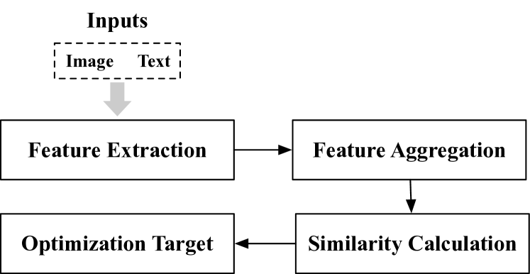
Figure 1: Illustration of VSE.

For feature aggregation, the most commonly used methods are simple pooling aggregators. MaxPool Wang et al. (2018) and MeanPool Reimers and Gurevych (2019) are designed to detect the salient and mean points of features, and K-MaxPool Kalchbrenner et al. (2014) extracts the mean of top-${\rm K}$ features. Some complex aggregation techniques have been proposed, e.g. local-importance projection Gao et al. (2019), sequence-to-sequence encoder Hu et al. (2019), graph convolution network Li et al. (2019), exponential adaptive pooling Stergiou and Poppe (2021) and self-attention encoder Wang et al. (2020). However, we found that carefully selected pooling functions can surpass complex methods (see Appendix A.1). Motivated by this, our paper proposes an approach that can automatically discover the best pooling functions. Specifically, we seek to improve the feature aggregation step by proposing a formulation that parameterizes the different pooling strategies and allows the model to learn the best configuration automatically via its objective, alleviating the need to do manual tuning. In other words, we’ve turned these hyper-parameters (i.e. choices of pooling functions) into parameters in the model.

For optimization, most VSE models optimize using the hinge triplet ranking loss with in-batch negative example Faghri et al. (2018). The intuition of the objective is to encourage positive pairs to be embedded in a similar space while widening the distance between a target with the hardest in-batch negative sample. In practice, however, it is often difficult for the model to find a good negative sample in the early stages of training (as instances are randomly distributed in space), resulting in slow convergence (see Appendix A.2). To improve optimization, we propose an adaptive optimization objective that selects multiple in-batch negative samples based on model quality during training. The intuition is that in the early stages of training we want to sample more negative samples, and in the later stages fewer negative samples.

Over two public datasets, MS-COCO Lin et al. (2014) and Flickr30K Young et al. (2014), we show that a standard VSE model using our proposed feature aggregation and optimization strategies outperforms benchmark models substantially. In particular, our method obtains 1.4% relative gains on RSUM for MS-COCO and 1.0% for Flickr30K. Compared with the pre-trained vision-language model with similar performance Geigle et al. (2022), our method is ${\rm 4.3\times}$ faster.

2 Related Work

Depending on whether the image and text features have any form of cross-modal interaction before similarity calculation, existing image-text retrieval can be broadly categorized into two types.

The visual semantic embedding (VSE) Faghri et al. (2018); Wang et al. (2020); Chun et al. (2021) methods process the multimodal instances independently before projecting them into a joint embedding space for similarity matching. Wang et al. (2018) design a two-branch neural networks, LIWE Wehrmann et al. (2019) considers character-based alignment and embedding methods for language encoder and Faghri et al. (2018) extend it by using hard triplet loss for optimization. Following these ideas, PVSE Song and Soleymani (2019) and CVSE Wang et al. (2020) are proposed to consider intra-modal polysemous and consensus information. Recently, Chun et al. (2021) samples instances as probabilistic distributions and achieves further improvement. These VSE-based methods are fast as they do not consider cross-modal interaction and as such the visual and text features can be pre-computed. The non-VSE methods concentrate on the interaction of modalities. Specially, late-interaction methods explore to fusion multi-modal information by attention Lee et al. (2018); Chen et al. (2020), alignment Zhang et al. (2020), multi-view representation Qu et al. (2020) and fine-grained reasoning Qu et al. (2021). The early-interaction methods Geigle et al. (2022), like pre-trained vision-language models Lu et al. (2019); Chen et al. (2019); Li et al. (2020); Jia et al. (2021); Li et al. (2022), focuses on the maximum of performance while sacrifices efficiency.

Our paper focuses on the improvement of feature aggregation and optimization for VSE. The existing explorations of those two steps are as follows.

The performance of VSE ultimately depends on the quality of the joint embedding space, which is usually learned with simple transformations (e.g. linear projection or multi-layer perceptron) and pooling aggregators (e.g. mean pooling Faghri et al. (2018); Qu et al. (2020), max pooling Zhang and Lu (2018); Li et al. (2021), or a combination of them Lee et al. (2018)). Compared to these simple aggregation methods, more complex aggregators that introduce a large number of trainable parameters have also been explored, e.g. inter-modal attention Wehrmann et al. (2020) and self-attention mechanisms Han et al. (2021). Zhang et al. (2021) design a cross-modal guided pooling module that attends to local information dynamically. These sophisticated aggregators typically require more time, and don’t always outperform simple pooling strategies. Perhaps the closest study to our work is GPO (VSE$\infty$) Chen et al. (2021), which builds a generalized operator to learn the best pooling strategy that only considers the position information of the extracted features.

Some studies focus on improving the optimization objective, and the most widely adopted objective is the hinge-based hard triplet ranking loss Faghri et al. (2018); Wei et al. (2020b); Messina et al. (2021), which dynamically selects the “hardest” negative sample within a mini-batch. Other studies explore solutions that choose multiple negative samples. Zhou et al. (2020) introduce a coherence metric to rank the “irrelevant” candidates. Extending the idea, Wei et al. (2020a) assign different weights for positive and negative pairs. To tackle the issue of noisy labels which impacts multimodal representation, Hu et al. (2021) propose maximizing the mutual information between different modalities. Huang et al. (2021) separate data into “clean” and “noisy” partitions by co-teaching. However, the above methods do not change adaptively according to the model performance when selecting negative samples.

3 Methodology

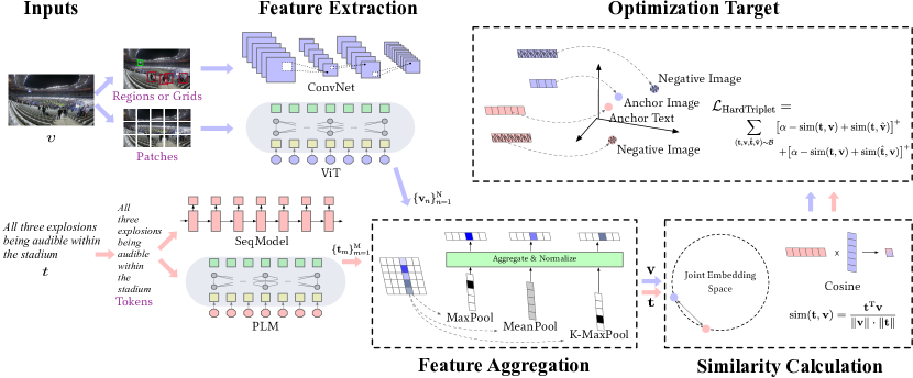
Figure 2: The framework of VSE. The visual and text encoders process the image and text separately at first. The related images and sentences are then directed to a similar space using an appropriate optimization target.

3.1 Background of VSE

We first discuss the standard formulation of VSE, before introducing our innovation on improving feature aggregation (Section 3.2) and optimization (Section 3.3).

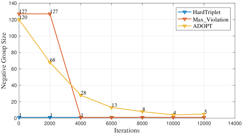
Figure 2: Visualization of negative group size learned by AdOpt on the first 5 epochs (about 12000 iterations).

To compute the similarity of given multimodal instance (image & text), a VSE model (Figure 2) separately encodes them via a visual encoder ($\mathtt{VisEnc}(\cdot)$) and a text encoder ($\mathtt{TextEnc}(\cdot)$). There are three widely used visual features produced by different visual encoders — grid is the feature maps from convolutional networks (CNNs; He et al. (2016)), region is the region of interest features from object detectors Anderson et al. (2018) and patch is the partition from vision transformer Dosovitskiy et al. (2021). The text encoders are usually RNNs Sutskever et al. (2014)) and BERT Devlin et al. (2019). Formally:

$$\textbf{F}_{v} =\mathtt{VisEnc}(v)$$

$$\textbf{F}_{t} =\mathtt{TextEnc}(t)$$

where $v$ and $t$ are the input image and text.

Assuming the visual feature $\textbf{F}_{v}$ has ${\rm N}$ object vectors (represented either as grids, regions or patches) in $d_{1}$ dimension, and the text feature $\textbf{F}_{t}$ has ${\rm M}$ token vectors in ${d_{2}}$ dimension, we next project them to the same $d$-dimension:

$$\{\textbf{v}_{n}\}^{\rm N}_{n=1}=\textbf{F}_{v}\textbf{W}_{v}+\textbf{b}_{v}$$ (1)

$$\{\textbf{t}_{m}\}^{\rm M}_{m=1}=\textbf{F}_{t}\textbf{W}_{t}+\textbf{b}_{t}$$

where $\mathbf{v}_{n}$ and $\mathbf{t}_{m}$ now have the same dimension $d$.

To aggregate the extracted features into fixed-length vectors, domain aggregators, $f_{\rm vision}(\cdot)$ and $f_{\rm text}(\cdot)$ are used to transform $\{\textbf{v}_{n}\}^{\rm N}_{n=1}\in\mathbb{R}^{{\rm N}\times d}$ and $\{\textbf{t}_{n}\}^{\rm M}_{m=1}\in\mathbb{R}^{{\rm M}\times d}$ into $\textbf{v}\in\mathbb{R}^{d}$ and $\textbf{t}\in\mathbb{R}^{d}$, respectively:

v $$=f_{\rm vision}\Big{(}\{\textbf{v}_{n}\}^{\rm N}_{n=1}\Big{)},$$

t $$=f_{\rm text}\Big{(}\{\textbf{t}_{m}\}^{\rm M}_{m=1}\Big{)}$$

And lastly, to measure how related the inputs we use cosine similarity:

$${\rm sim}(\textbf{t},\textbf{v})=\frac{\textbf{t}^{\mathrm{T}}\textbf{v}}{\|\textbf{t}\|\cdot\|\textbf{v}\|}$$

Existing optimization strategies generally use the hinge-based triplet ranking loss to optimize the VSE model. Given an anchor, it aims to maximize its similarity with positive samples while minimizing its similarity with the most “difficult” negative sample in the mini-batch (i.e. the example that has the highest similarity with the anchor that is not a positive example), and includes both text-to-image and image-to-text retrieval objectives:

$$\mathcal{L}_{\rm HardTriplet} =$$ (2)

$$\sum_{(\textbf{t},\textbf{v},\hat{\textbf{t}},\hat{\textbf{v}})\sim\mathcal{B}} \big{[}\alpha-{\rm sim}(\textbf{t},\textbf{v})+{\rm sim}(\textbf{t},\hat{\textbf{v}})\big{]}^{+}$$

$$+\big{[}\alpha-{\rm sim}(\textbf{t},\textbf{v})+{\rm sim}(\hat{\textbf{t}},\textbf{v})\big{]}^{+}$$

where $\alpha$ is the margin hyper-parameter, and $[x]^{+}=\mathrm{max}(0,x)$. $(\textbf{t},\textbf{v})$ is a positive text-image pair in mini-batch $\mathcal{B}$ and $(\hat{\textbf{t}},\textbf{v})$ and $(\textbf{t},\hat{\textbf{v}})$ are negative pairs, where $\hat{\textbf{t}}=\mathrm{argmax}_{\textbf{t}^{\prime}\neq\textbf{t}}{\rm sim}(\textbf{t}^{\prime},\textbf{v})$ and $\hat{\textbf{v}}=\mathrm{argmax}_{\textbf{v}^{\prime}\neq\textbf{v}}{\rm sim}(\textbf{t},\textbf{v}^{\prime})$ are the hardest negative sentence and image respectively in $\mathcal{B}$.

3.2 Enhancing VSE by Adaptive Pooling

We now describe our approach (named adaptive pooling, AdPool) to improving feature aggregation, where we parameterize the pooling operations ($f_{\rm vision}$ and $f_{\rm text}$) to allow VSE to learn the best way to aggregate the features via its objective adaptively (in other words, we have effectively turned the pooling methods — which are hyper-parameters — into model parameters). Our approach has the advantage of being much faster and simpler than complex aggregators, as it introduces only a small number of parameters. Note that we will describe our method only for the text feature ($\{\textbf{t}_{m}\}^{\rm M}_{m=1}$), as the same process can be applied for the visual feature ($\{\textbf{v}_{n}\}^{\rm N}_{n=1}$).

3.2.1 Token-level Pooling

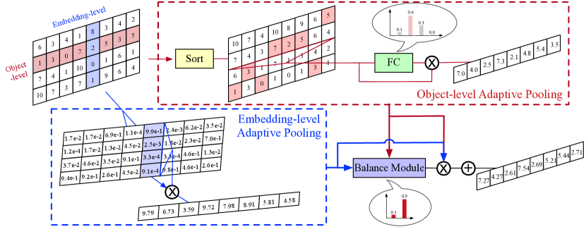
Figure 3: Illustration of our proposed adaptive pooling module (AdPool). It produces vectors pooled at the Token-level and embedding-level and combined via a balance module. Each red row denotes a token in a sentence.

Recall that the text feature ($\{\textbf{t}_{m}\}^{\rm M}_{m=1}$) has ${\rm M}$ tokens each of $d$-dimension. The exact form of $\textbf{t}_{m}$ can be token vectors. As for vision features, they can be grids, regions or image patches, depending on the visual encoder. Let $\mathrm{max}_{k}(\cdot)$ be a function that extracts the top $k$-th value in a list, the common pooling mechanisms can be formulated as a "sort $\rightarrow$ weight-sum" paradigm Grefenstette et al. (2014) as following:

• MeanPool = $\frac{1}{\rm M}\sum^{\rm M}_{i=1}\{{t}_{ij}\}^{\rm M}_{i=1}$ ouputs the mean value among ${\rm N}$ objects at position $j$;

• MaxPool = $\mathrm{max}_{1}\big{(}\{{t}_{ij}\}^{\rm M}_{i=1}\big{)}$ returns the maximum values of $\{{t}_{ij}\}^{\rm M}_{i=1},\forall{j}$;

• K-MaxPool = $\frac{1}{\rm K}\sum^{\rm K}_{k=1}\mathrm{max}_{k}\big{(}\{{t}_{ij}\}^{\rm M}_{i=1}\big{)}$ computes the mean of the top-${\rm K}$ values.

where $t_{ij}$ denotes the $j$-th element in the $i$-th token vector.

Using the token vectors $\{\textbf{t}_{m}\}^{\rm M}_{m=1}$ in Figure 3 (red rows in the input matrix) as an example, we follow the "sort $\rightarrow$ weight-sum" paradigm of simple pooling methods to first sort the feature matrix along the embedding axis. Next we let the model learn (via a fully-connected layer) how to weight each vector (red rows in the matrix) automatically (e.g. $[0.1,0.6,0.3,0.0]$ in Figure 3). In this way, we allow the model to find the best combination of MeanPool and K-MaxPool in an adaptive manner. Formally as:

$$\textbf{t}^{\rm tok} =\sum^{\rm M}_{m=1}\theta_{m}\cdot\textbf{u}_{m}$$ (3)

$$\{\textbf{u}_{m}\}^{\rm M}_{m=1} =\mathrm{sort}\big{(}\{\textbf{t}_{m}\}^{\rm M}_{m=1}\big{)}$$

$$\bm{\theta} =\mathrm{softmax}\left(\{\textbf{u}_{m}\}^{\rm M}_{m=1}\textbf{W}_{\rm tok}\right)$$

where $\mathrm{sort(\cdot)}$ is a function that sorts the token vectors along the embedding axis.

3.2.2 Embedding-level Pooling

With token-level pooling, we learn to how to weight each (sorted) token vector and aggregate them. With embedding-pooling, we learn how to weight each (original unsorted) object vector in each embedding dimension to extract the most salient element within that dimension, and can be interpreted as a “soft” version of MaxPool:

$$\textbf{t}^{\rm emb} =\sum^{\rm M}_{i=1}\delta_{ij}\cdot{t}_{ij},\forall{j}$$ (4)

$$\delta_{ij} =\frac{e^{{t}_{ij}}}{\sum^{\rm M}_{i=1}e^{{t}_{ij}}},\forall{i}$$

3.2.3 Combining Token-level and Embedding-level Pooled Vectors

Given the two pooled vectors $\textbf{t}^{\rm tok}$ and $\textbf{t}^{\rm emb}$ (which have the same dimension $d$), one straightforward way to combine them is to weight them with scaling hyper-parameters. To avoid these hyper-parameters (which requires manual tuning), we let the model learn these weights automatically with a trainable $\textbf{W}_{bal}\in\mathbb{R}^{d\times 1}$:

t $$=\omega_{1}\textbf{t}^{\rm tok}+\omega_{2}\textbf{t}^{\rm emb}$$ (5)

$$\mathbf{\omega_{\{1,2\}}} =\text{softmax}\Big{(}[\textbf{t}^{\rm tok}\textbf{W}_{bal},\textbf{t}^{\rm emb}\textbf{W}_{bal}]\Big{)}$$

For the visual feature $\{\textbf{v}_{n}\}^{\rm N}_{n=1}$ (Equation 1), we follow the same process to compute the token-level (where here an “token” is a unit of image) and embedding-level pooled vectors ($\textbf{v}^{\rm tok}$ and $\textbf{v}^{\rm emb}$) and combine them to produce $\textbf{v}\in\mathbb{R}^{d}$.

3.3 Enhancing VSE by Adaptive Objective

Our next contribution is in improving the optimization step. The hard triplet loss (Equation 2) is the most commonly utilized training objective for optimizing VSE. However, we find that locating a “difficult” negative sample is challenging in the early stages of training (Appendix A.2), resulting in delayed convergence. We introduce a novel adaptive optimization objective, AdOpt, that automatically (or adaptively) selects ${\rm K}$ ${\rm(K\geq 1)}$ negative samples in each mini-batch $\mathcal{B}$ during training.

Wang and Isola (2020) introduce two key properties, Alignment and Uniformity, that correlate with a retrieval performance:

• Alignment: the positive $(\textbf{t}$ and $\textbf{v})$ should be mapped into a similar embedding space. Defining $\gamma_{\rm align}\in[0,1]$ as the average similarity values for all positive pairs, the larger $\gamma_{\rm align}$ is, the better the VSE model.

  $$\gamma_{\rm align}=\mathop{\mathbb{E}}\limits_{(\textbf{t},\textbf{v})\sim\mathcal{B}}[{\rm sim}(\textbf{t},\textbf{v})]$$

• Uniformity: all vectors should be roughly uniformly distributed on the unit hypersphere, and $\gamma_{\rm uniform}\in[0,1]$ measures this quality.

  $$\gamma_{\rm uniform}=\mathrm{log}\mathop{\mathbb{E}}\limits_{\textbf{t}\sim\mathcal{B},\textbf{v}\sim\mathcal{B}}[e^{{\rm sim}(\textbf{t},\textbf{v})}]$$

By combining $\frac{(\gamma_{\rm align}+\gamma_{\rm uniform})\times\pi}{4}\in[0,\frac{\pi}{2}]$, we can use it to assess the maturity of a VSE model during training and dynamically adjust the number of negative samples. That is, in the early stages of training, we expect the value to be close to 0 (as the model is unable to differentiate between positive and negative samples), and we would want to use more negative samples for optimization. Conversely in the later stages of training, the value should be close to $\frac{\pi}{2}$ and we want less negative samples. Formally:

$${\rm K}^{\prime} =\rm{round}\Big{(}|\mathcal{B}|\times\mathrm{cos}(\frac{(\gamma_{\rm align}+\gamma_{\rm uniform})\times\pi}{4})\Big{)}$$ (6)

$$\rm{K} =\rm{max}\Big{(}1,\rm{min}(\rm{K}^{\prime},|\mathcal{B}|-1)\Big{)}$$

where $\rm{cos}$ is the cosine function to invert the sum, $\rm{K}$ is the number of negative samples to be used, and ${\rm round}(x)$ is a function that rounds down the value of $x$. As the hard triplet loss can only work with ${\rm K}=1$ (Equation 2), we therefore utilize the InfoNCE objective Van den Oord et al. (2018), which is a commonly used contrastive objective Radford et al. (2021):

$$\mathcal{L}=\mathcal{L}_{\rm v2t}+\mathcal{L}_{\rm t2v}$$

$$\mathcal{L}_{\rm v2t}=-\frac{1}{|\mathcal{B}|}\sum_{(\textbf{t},\textbf{v})\in\mathcal{B}}\mathrm{log}\frac{\mathrm{exp\big{(}\mathrm{sim}(\textbf{t},\textbf{v})/\tau\big{)}}}{\sum^{\rm K}_{k}\mathrm{exp}\big{(}\mathrm{sim}(\hat{\textbf{t}}_{k},\textbf{v})/\tau\big{)}}$$

$$\mathcal{L}_{\rm t2v}=-\frac{1}{|\mathcal{B}|}\sum_{(\textbf{t},\textbf{v})\in\mathcal{B}}\mathrm{log}\frac{\mathrm{exp\big{(}\mathrm{sim}(\textbf{t},\textbf{v})/\tau\big{)}}}{\sum^{\rm K}_{k}\mathrm{exp}\big{(}\mathrm{sim}(\textbf{t},\hat{\textbf{v}}_{k})/\tau\big{)}}$$

where $\tau$ is the temperature hyper-parameter.

4 Experiments

4.1 Datasets and Metrics

Datasets. We conduct our experiments on MS-COCO and Flickr30K using various visual and text encoders for cross-modal retrieval. The MS-COCO dataset contains 123,287 images, each with 5 manually annotated sentences. Following the split method of Faghri et al. (2018), 113,287 images are used for training, 5,000 for validation, and 5,000 for testing.

Following prior studies Faghri et al. (2018), we experiment with two evaluation settings: (1) MS-COCO 1K averages the results over 5-folds of 1K test images; and (2) MS-COCO 5K directly results on the whole 5K test images. Following Chen et al. (2021), we use the former to assess overall performance with state-of-the-art VSE models and the latter for further analyses such as ablation results. Flickr30K consists of 31,783 images with the same corresponding 5 captions, and 1,000 images are reserved for validation and testing.

Metrics. We evaluate cross-modal retrieval performance using recall@K (R@K), where ${\rm K}=\{1,5,10\}$. The evaluation tasks include both caption retrieval (given caption, find images) and image retrieval (given image, find captions). We also compute RSUM which is a sum of all R@K metrics across both tasks to assess the overall performance.

		MS-COCO 5-fold 1K Test
		Image Retrieval			Caption Retrieval
VF	Method	R@1	R@5	R@10	R@1	R@5	R@10	RSUM
	Text Encoder: BiGRU
R	VSE++	54.0	85.6	92.7	68.5	92.6	97.1	490.5
R	LIWE	57.9	88.3	94.5	73.2	95.5	98.2	507.6
R	PVSE	55.2	86.5	93.7	69.2	91.6	96.6	492.8
R	CVSE	55.7	86.9	93.8	69.2	93.3	97.5	496.4
R	VSE$\infty$	61.7	90.3	95.6	78.5	96.0	98.7	520.5
R	SCAN(i2t)	54.4	86.0	93.6	69.2	93.2	97.5	493.9
R	SCAN(t2i)	56.4	87.0	93.9	70.9	94.5	97.8	500.5
R	CAAN	61.3	89.7	95.2	75.5	95.4	98.5	515.6
R	IMRAM	61.7	89.1	95.0	76.7	95.6	98.5	516.6
R	VSE+2AD	63.5	91.8	96.3	79.7	97.3	99.2	527.8
1-9[1pt/1pt] RG	VSE$\infty$	64.8	91.6	96.5	80.0	97.0	99.0	528.8
RG	VSE+2AD	65.7	92.3	97.0	82.1	97.9	99.4	534.4
1-9[1pt/1pt] RGP	VSE+2AD	67.1	93.0	97.7	83.8	98.1	99.4	539.1
	Text Encoder: BERT
R	VSE++	54.0	85.6	92.5	67.9	91.9	97.0	488.9
R	VSE$\infty$	64.8	91.4	96.3	79.7	96.4	98.9	527.5
R	DSRN	64.5	90.8	95.8	78.3	95.7	98.4	523.5
R	DIME(i2t)	63.0	90.5	96.2	77.9	95.9	98.3	521.8
R	DIME(t2i)	62.3	90.2	95.8	77.2	95.5	98.5	519.5
R	VSE+2AD	67.5	93.6	97.7	81.3	96.7	99.2	536.0
1-9[1pt/1pt] RG	VSE$\infty$	68.1	92.9	97.2	82.2	97.5	99.5	537.4
RG	VSE+2AD	71.9	94.3	98.3	84.2	98.5	99.4	546.6
1-9[1pt/1pt] RGP	VSE+2AD	72.5	94.8	98.7	85.4	98.9	99.2	549.5

Flickr30K 1K Test
Image Retrieval			Caption Retrieval
R@1	R@5	R@10	R@1	R@5	R@10	RSUM
45.7	73.6	81.9	62.2	86.6	92.3	442.3
51.2	80.4	87.2	69.6	90.3	95.6	474.3
-	-	-	-	-	-	-
54.7	82.2	88.6	70.5	88.0	92.7	476.7
56.4	83.4	89.9	76.5	94.2	97.7	498.1
43.9	74.2	82.8	67.9	89.0	94.4	452.2
45.8	74.4	83.0	61.8	87.5	93.7	446.2
52.8	79.0	87.9	70.1	91.6	97.2	478.6
53.9	79.4	87.2	74.1	93.0	96.6	484.2
58.0	85.0	91.2	76.9	94.4	98.2	503.7
1-7[1pt/1pt] 60.8	86.3	92.3	80.7	96.4	98.3	514.8
62.2	86.8	93.1	82.2	97.1	98.8	520.2
1-7[1pt/1pt] 63.5	87.6	93.4	83.1	97.7	99.1	524.4
45.6	76.4	84.4	63.4	87.2	92.7	449.7
61.4	85.9	91.5	81.7	95.4	97.6	513.5
59.2	86.0	91.9	77.8	95.1	97.6	507.6
64.6	85.5	91.0	77.5	93.5	97.4	504.0
60.1	85.5	91.8	77.4	95.0	97.4	507.2
59.1	90.3	93.5	81.8	96.1	98.4	524.7
1-7[1pt/1pt] 66.7	89.9	94.0	85.3	97.2	98.9	532.0
69.2	91.3	95.6	87.1	97.9	99.3	540.4
1-7[1pt/1pt] 71.4	92.0	95.8	88.2	98.4	99.5	545.3

Table 1: Cross-modal retrieval results on MS-COCO and Flickr30K datasets. The top half of the table uses BiGRU as the text encoder; the bottom half is BERT. VF denotes vision feature, and R, G, and P mean region, grid and patch respectively. The best results are marked bold in black, blue and red for region feature (R), ensemble of region$+$grid features (RG) and ensemble of region$+$grid$+$patch features (RGP) respectively. VSE+2AD is our proposed model, which enhances the VSE model by using AdPool for aggregation and AdOpt for optimization.

4.2 Implementation Details

We implement our models using the PyTorch library. The dimension of the shared embedding space $d$ is 1024. We use the Adam optimizer with a mini-batch size of 128 and train our models with 25 epochs. The learning rate is set to 5e-4 with a decaying factor of 10% for every 15 epochs.

Visual Encoders. We use Faster-RCNN Ren et al. (2015) (ResNet-101 is pre-trained on ImageNet and Visual Genome) to extract region feature directly Anderson et al. (2018), and fine-tune it further with grid feature (resolution $=$ 512$\times$512) Jiang et al. (2020) before using it as a grid feature extractor. For the patch feature, we fine-tune the pre-trained Vision Transformer Dosovitskiy et al. (2021) using images with a resolution of 224$\times$224 to use it as a patch feature extractor.

Text Encoders. We experiment with BiGRU Faghri et al. (2018) and BERT-base Devlin et al. (2019). Additional implementation and training details are given in the Appendix.

4.3 Main Results

Table 1 presents the full results over both image and caption retrieval and across two datasets (MS-COCO and Flickr30K). Results for MS-COCO is an average of over 5-folds of 1K test images. Our method is “VSE+2AD”, which enhances the standard VSE model by introducing AdPool and AdOpt. The top half of the table presents results where we use BiGRU as the text encoder, and the bottom half uses BERT. For models where we combine visual features from multiple visual encoders (e.g. “RG” which combines region and grid feature), we do so by simply taking the average similarity values to rank the candidates.

Looking at the results, VSE+2AD (our model) outperforms almost all baselines/benchmark models consistently. Our model displays consistent improvement over the state-of-the-art method VSE$\infty$ Chen et al. (2021) with the same visual (region feature by BUTD Anderson et al. (2018)) and text encoders (BiGRU). In particular, it obtains 1.4% (520.5 $\rightarrow$ 527.8) and 1.0% (498.1 $\rightarrow$ 503.1) relative gains on RSUM for MS-COCO and Flickr30K datasets. Such improvements are stable no matter using which combination of visual and text encoders. We also see that combining visual encoders (“RG” vs. “R”) further boosts its performance (like RSUM from 527.8 to 534.4 for the MS-COCO dataset), and utilizing all types of visual features (“RGP”) produces the best performance (539.1 $\textgreater$ 534.4 $\textgreater$ 527.8).

4.4 Comparison with pre-trained models

We next compare VSE+2AD (with BERT as the language encoder) to pre-trained vision language models: ViLBERT Lu et al. (2019), UNITER Chen et al. (2019), OSCAR Li et al. (2020), ALIGN Jia et al. (2021), CLIP Radford et al. (2021) and MVP Li et al. (2022) in Table 2. These results are evaluated on the COCO 5K test images.

Without using any large-scale corpus for pre-training, our ensemble VSE+2AD${}^{\text{RGP}}$ (that combines region/grid/patch features) outperforms two out of six pre-trained VL methods and is not much worse than OSCAR, even though it does not use any cross-modal interaction. Our model is substantially faster than these pre-trained models: our slowest ensemble model is still an order of magnitude faster. As for our method we can pre-compute and cache the visual and text features, so during retrieval the only operations needed are similarity calculation and ranking. Overall, these results demonstrate that our model strikes a good balance between performance and efficiency.

	COCO 5K Test
	Image Retrieval		Caption Retrieval
Method	R@1	R@5	R@1	R@5	RSUM	#OIPs
ViLBERT	38.6	68.2	53.5	79.7	406.9	-
UNITER	48.4	76.7	63.3	87.0	454.4	9.6$\times$
OSCAR	54.0	80.8	70.0	91.1	479.9	4.3$\times$
ALIGN	59.9	83.3	77.0	93.5	500.4	1.0$\times$
CLIP	58.7	83.6	76.8	94.0	500.9	-
MVP	60.1	84.0	77.3	93.6	502.6	-
1-7[1pt/1pt] VSE+2AD	52.5	80.2	69.5	91.2	475.9	45.3$\times$

Table 2: Comparison between VSE+2AD and pre-trained models. #OIPs denotes operating items per second, and larger is better. The language encoder for VSE+2AD is BERT. And the shown number is the ensemble results considering region$+$grid$+$patch visual features.

	COCO 5K Test
	Image Retrieval			Caption Retrieval
Method	R@1	R@5	R@10	R@1	R@5	R@10	RSUM
VSE+2AD	41.4	72.3	83.8	54.9	83.0	91.5	426.9
1-8[1pt/1pt] $-$tok AdPool	39.5	71.3	82.3	53.5	82.2	91.3	420.1
$-$emb AdPool	40.1	72.3	83.2	53.7	82.5	91.3	423.1
$-$AdPool	38.5	72.4	81.8	53.3	82.0	91.1	419.1
1-8[1pt/1pt] $-$AdOpt	39.2	71.1	81.5	53.4	82.2	90.5	417.9

Table 3: Ablation results where we measure the token-level, embedding-level, overall AdPool pooling methods and AdOpt optimization strategy. The region feature with simple projection as visual encoder and BiGRU as the textual encoder.

4.5 Ablation Study

To understand the impact of AdPool (which improves feature aggregation in Section 3.2) and AdOpt (which improves optimization in Section 3.3), we perform several ablation studies based on the COCO 5K test. For this experiment (in Table 3), we use only the region feature and BiGRU as the text encoder. Looking at the aggregate RSUM performance, we see both the token-level pooling (“$-$tok AdPool”; Section 3.2.1) and embedding-level pooling (“$-$emb AdPool”; Section 3.2.2) appear to be useful, although token-level pooling is arguably more important. In the case where we remove AdPool entirely (“$-$AdPool”) and use MeanPool as the aggregation method, the performance drops even more, suggesting complementarity. AdOpt is the most impactful method, where taking it out produces the worst performance. To understand its impact qualitatively, we also look at the training curve of a VSE model trained with and without AdOpt (Appendix A.2 Figure 1). Here it is clear that AdOpt is particularly useful in the early stages of training, where it helps the model to converge much faster. This earlier convergence ultimately impacts their final performance, where the VSE trained with AdOpt reaches a plateau that is higher than the one without AdOpt.

We next investigate the impact of AdPool further, by replacing it with other more advanced pooling strategies. As before, we use the region feature, BiGRU for text encoder, and COCO 5K test. Table 4 presents the results. Here we see that AdPool outperforms existing pooling strategies (best RSUM), even against more complex aggregators such as Seq2Seq, GCN and SelfAttn. It is also reasonably fast (competitive with other methods). These results once again highlight that our proposed pooling method has both performance and speed as we saw in Section 4.4.

	COCO 5K Test
	Image Retrieval		Caption Retrieval
Aggregator	R@1	R@5	R@1	R@5	RSUM	#OIPs
LIP	38.4	69.3	52.2	81.1	414.8	4.6$\times$
Seq2Seq	38.2	68.9	52.1	80.9	415.7	1.8$\times$
GCN	40.7	71.3	53.5	81.5	419.2	1.0$\times$
SelfAttn	40.9	71.3	53.8	82.2	420.1	1.6$\times$
AdaPool	40.2	71.8	52.8	81.4	418.3	4.1$\times$
SoftPool	39.2	69.8	52.8	81.4	419.8	5.1$\times$
GPO	41.2	71.1	55.6	82.0	422.9	4.3$\times$
Manual	38.7	71.6	53.7	82.1	419.3	5.6$\times$
1-8[1pt/1pt] AdPool	41.4	72.3	54.9	83.0	426.9	4.9$\times$

Table 4: Performance of VSE+2AD using different aggregators. #OIPs denotes operating items per second, and larger is better. Note that our proposed AdPool aggregation method is only slower than simple pooling, 5.6$\times\textgreater$ 4.9 $\times(\textsc{AdPool})\textgreater$ others, but it no need for fussily manual tuning.

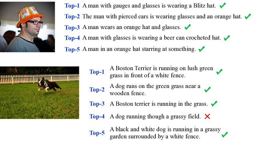
(a) Image Retrieval

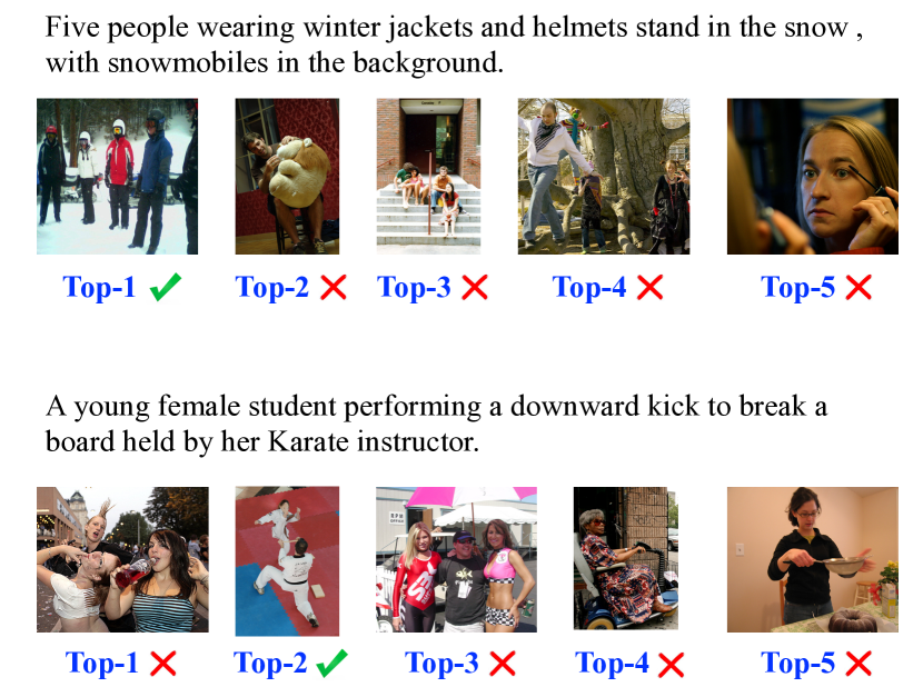
(b) Caption Retrieval

Figure 4: Top-5 image retrieval and caption retrieval results on Flickr30K. The ground-truth results are marked with greed $\checkmark$, and the wrong results are indicated by red $\usym{2718}$.

4.6 Case Study

To validate the effectiveness of VSE+2AD, we present two examples for image retrieval and caption retrieval in Figure 4(a) and Figure 4(b), respectively. As we can see in Figure 4(a), the “incorrect” sentence retrieved by our model seems sensible, suggesting that this is likely noise in the data. Figure 4(b), on the other hand, shows some genuine erroneous images retrieved by our model, and we suspect this is because it is a particularly difficult example where the caption is very descriptive and the details are difficult to be captured by VSE’s bi-encoder approach.

5 Conclusion

In this paper, we propose methods to improve VSE’s feature aggregation and optimization objective. For the former, we introduce a way to parameterize the aggregation function to allow the visual and text encoders to learn the best way to combine their features to produce a fixed-size embedding. For the latter, we propose a method that dynamically selects many negative samples that allows the VSE to converge faster with a better final performance. We compare our enhanced VSE model to several baselines and state-of-the-art models over two public datasets and demonstrate that it marries both performance (state-of-the-art retrieval results) and efficiency (orders of magnitude faster than pretrained models). As our proposed method is more suitable for practical application.

Appendix

Appendix A Verification of Assumptions

A.1 Simple pooling strategy works best

Although various complex methods (described in Section 2) are explored for aggregation, we find that the simple pooling strategy works no worse than those complex methods by numerous experiments. It needs to be carefully manually tuned, like 5-MaxPool for visual feature and MeanPool for text feature. The results are shown in Table A.1-1, where the similar conclusion is also verified in VSE$\infty$ Chen et al. (2021).

	COCO 5K Test
	Image Retrieval		Caption Retrieval
Aggregator	R@1	R@5	R@1	R@5	RSUM
LIP	38.4	69.3	52.2	81.1	414.8
Seq2Seq	38.2	68.9	52.1	80.9	415.7
GCN	40.7	71.3	53.5	81.5	419.2
SelfAttn	40.9	71.3	53.8	82.2	420.1
AdaPool	40.2	71.8	52.8	81.4	418.3
SoftPool	39.2	69.8	52.8	81.4	419.8
GPO	41.2	71.1	55.6	82.0	422.9
Manual	38.7	71.6	53.7	82.1	419.3

Table 1: Comparison of complex aggregators and manually chosen pooling method evaluated with MS-COCO 5K.

A.2 Hardest triplet loss slows the convergence

Figure A.2-1 shows the comparison of VSE model with and without our proposed optimization objective, AdOpt. Note that hard triplet loss Faghri et al. (2018) is used for optimization when AdOpt is not used. The optimization target AdOpt can fit the model more quickly, thus further improving the potential of the model, that is performance is better in the latter stage.

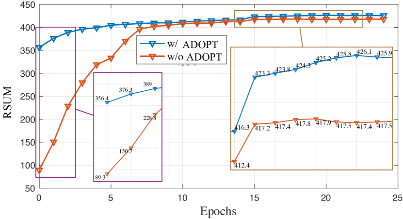
Figure 1: Performance of VSE trained with and without AdOpt.

Appendix B Additional Implementation Details

Basic settings. The margin $\alpha$ for hard triplet loss is set to 0.2 and the $\tau$ used in InfoNCE is 0.05. The image and text features extracted from the encoders use L2 normalization. The common learning rate is set to 5e-4, while the learning rate of the pre-trained modules (like BERT, ResNet and ViT) is 10% of its.

Vision Encoders. When using region feature that directly extracted from BUTD Anderson et al. (2018), the multilayer perceptron is used to map the visual feature dimension into 1024 as the same as text feature dimension. For grid feature, the warm-up strategy is used for the first epoch. Then, all parameters are optimized in the rest of 24 epochs. For patch feature, the original image is changed to 224$\times$224 resolution with the size of a patch as 16.

Language Encoders. When using BiGRU as the backbone, the token dimension is 300 and the hidden dimension is 1024. Only one layer is considered and the bidirectional features are averaged as the output feature. For BERT, the hidden dimension is 768 and the multilayer perceptron is also used to map the text feature dimension into 1024 as the same as visual feature dimension.

Appendix C Additional Experiments and Results

We present Figure C-2 to show how the size of the negative samples changes during training with AdOpt. We can see that AdOpt starts with a large number of negative samples, but that decreases over time to only 4–5 samples at the end of the 5^th epoch (yellow line). Different from the common hard triplet optimization that only considers one hardest negative sample, the max_violation strategy Faghri et al. (2018) considers the rest samples within the same mini-batch as negative samples only on the first epoch and the rest epochs are the same as the hard triplet loss.

We last investigate the impact of the balance module in AdPool (Equation 5). Table C-2 shows that manually tuned weights underperform substantially compared to automatically learned weights.

		COCO 5K Test
Weights		Image Retrieval		Caption Retrieval
obj	emb	R@1	R@5	R@1	R@5	RSUM
0.25	0.75	39.8	70.2	51.9	80.4	416.6
0.5	0.5	40.1	70.6	52.8	81.1	418.2
0.75	0.25	40.6	71.4	54.1	82.2	421.3
random	random	39.3	69.4	51.2	80.1	413.9
1-7[1pt/1pt] AdPool	AdPool	41.4	72.3	54.9	83.0	426.9

Table 2: Different choices of parameters for fusing token-level and embedding-pooling.

References

- Anderson et al. (2018) Peter Anderson, Xiaodong He, Chris Buehler, Damien Teney, Mark Johnson, Stephen Gould, and Lei Zhang. 2018. Bottom-up and top-down attention for image captioning and visual question answering. In Proceedings of the IEEE conference on computer vision and pattern recognition, pages 6077–6086.
- Chen et al. (2020) Hui Chen, Guiguang Ding, Xudong Liu, Zijia Lin, Ji Liu, and Jungong Han. 2020. Imram: Iterative matching with recurrent attention memory for cross-modal image-text retrieval. In Proceedings of the IEEE/CVF conference on computer vision and pattern recognition, pages 12655–12663.
- Chen et al. (2021) Jiacheng Chen, Hexiang Hu, Hao Wu, Yuning Jiang, and Changhu Wang. 2021. Learning the best pooling strategy for visual semantic embedding. In Proceedings of the IEEE/CVF Conference on Computer Vision and Pattern Recognition, pages 15789–15798.
- Chen et al. (2019) Yen-Chun Chen, Linjie Li, Licheng Yu, Ahmed El Kholy, Faisal Ahmed, Zhe Gan, Yu Cheng, and Jingjing Liu. 2019. Uniter: Learning universal image-text representations.
- Chun et al. (2021) Sanghyuk Chun, Seong Joon Oh, Rafael Sampaio De Rezende, Yannis Kalantidis, and Diane Larlus. 2021. Probabilistic embeddings for cross-modal retrieval. In Proceedings of the IEEE/CVF Conference on Computer Vision and Pattern Recognition, pages 8415–8424.
- Devlin et al. (2019) Jacob Devlin, Ming-Wei Chang, Kenton Lee, and Kristina Toutanova. 2019. BERT: Pre-training of deep bidirectional transformers for language understanding. In Proceedings of the 2019 Conference of the North American Chapter of the Association for Computational Linguistics: Human Language Technologies, Volume 1 (Long and Short Papers), pages 4171–4186, Minneapolis, Minnesota. Association for Computational Linguistics.
- Dosovitskiy et al. (2021) Alexey Dosovitskiy, Lucas Beyer, Alexander Kolesnikov, Dirk Weissenborn, Xiaohua Zhai, Thomas Unterthiner, Mostafa Dehghani, Matthias Minderer, Georg Heigold, Sylvain Gelly, Jakob Uszkoreit, and Neil Houlsby. 2021. An image is worth 16x16 words: Transformers for image recognition at scale. ICLR.
- Faghri et al. (2018) Fartash Faghri, David J Fleet, Jamie Ryan Kiros, and Sanja Fidler. 2018. Vse++: Improving visual-semantic embeddings with hard negatives. Proceedings of the British Machine Vision Conference (BMVC).
- Frome et al. (2013) Andrea Frome, Greg S Corrado, Jon Shlens, Samy Bengio, Jeff Dean, Marc’Aurelio Ranzato, and Tomas Mikolov. 2013. Devise: A deep visual-semantic embedding model. Advances in neural information processing systems, 26.
- Gao et al. (2019) Ziteng Gao, Limin Wang, and Gangshan Wu. 2019. Lip: Local importance-based pooling. In 2019 IEEE/CVF International Conference on Computer Vision (ICCV), pages 3354–3363.
- Geigle et al. (2022) Gregor Geigle, Jonas Pfeiffer, Nils Reimers, Ivan Vulić, and Iryna Gurevych. 2022. Retrieve Fast, Rerank Smart: Cooperative and Joint Approaches for Improved Cross-Modal Retrieval. Transactions of the Association for Computational Linguistics, 10:503–521.
- Grefenstette et al. (2014) Edward Grefenstette, Phil Blunsom, et al. 2014. A convolutional neural network for modelling sentences. In The 52nd Annual Meeting of the Association for Computational Linguistics, Baltimore, Maryland.
- Han et al. (2021) Ning Han, Jingjing Chen, Guangyi Xiao, Hao Zhang, Yawen Zeng, and Hao Chen. 2021. Fine-grained cross-modal alignment network for text-video retrieval. In Proceedings of the 29th ACM International Conference on Multimedia, pages 3826–3834.
- He et al. (2016) Kaiming He, Xiangyu Zhang, Shaoqing Ren, and Jian Sun. 2016. Deep residual learning for image recognition. In Proceedings of the IEEE conference on computer vision and pattern recognition, pages 770–778.
- Hu et al. (2019) Hexiang Hu, Ishan Misra, and Laurens van der Maaten. 2019. Evaluating text-to-image matching using binary image selection (bison). In Proceedings of the IEEE/CVF International Conference on Computer Vision Workshops, pages 0–0.
- Hu et al. (2021) Peng Hu, Xi Peng, Hongyuan Zhu, Liangli Zhen, and Jie Lin. 2021. Learning cross-modal retrieval with noisy labels. In Proceedings of the IEEE/CVF Conference on Computer Vision and Pattern Recognition, pages 5403–5413.
- Huang et al. (2021) Zhenyu Huang, Guocheng Niu, Xiao Liu, Wenbiao Ding, Xinyan Xiao, Hua Wu, and Xi Peng. 2021. Learning with noisy correspondence for cross-modal matching. Advances in Neural Information Processing Systems, 34.
- Jia et al. (2021) Chao Jia, Yinfei Yang, Ye Xia, Yi-Ting Chen, Zarana Parekh, Hieu Pham, Quoc V. Le, Yun-Hsuan Sung, Zhen Li, and Tom Duerig. 2021. Scaling up visual and vision-language representation learning with noisy text supervision. In ICML.
- Jiang et al. (2020) Huaizu Jiang, Ishan Misra, Marcus Rohrbach, Erik Learned-Miller, and Xinlei Chen. 2020. In defense of grid features for visual question answering. In Proceedings of the IEEE/CVF Conference on Computer Vision and Pattern Recognition, pages 10267–10276.
- Kalchbrenner et al. (2014) Nal Kalchbrenner, Edward Grefenstette, and Phil Blunsom. 2014. A convolutional neural network for modelling sentences. In Proceedings of the 52nd Annual Meeting of the Association for Computational Linguistics (Volume 1: Long Papers), pages 655–665, Baltimore, Maryland. Association for Computational Linguistics.
- Lee et al. (2018) Kuang-Huei Lee, Xi Chen, Gang Hua, Houdong Hu, and Xiaodong He. 2018. Stacked cross attention for image-text matching. In Proceedings of the European Conference on Computer Vision (ECCV), pages 201–216.
- Li et al. (2021) Jiangtong Li, Liu Liu, Li Niu, and Liqing Zhang. 2021. Memorize, associate and match: Embedding enhancement via fine-grained alignment for image-text retrieval. IEEE Transactions on Image Processing, 30:9193–9207.
- Li et al. (2019) Kunpeng Li, Yulun Zhang, Kai Li, Yuanyuan Li, and Yun Fu. 2019. Visual semantic reasoning for image-text matching. In Proceedings of the IEEE/CVF International conference on computer vision, pages 4654–4662.
- Li et al. (2020) Xiujun Li, Xi Yin, Chunyuan Li, Pengchuan Zhang, Xiaowei Hu, Lei Zhang, Lijuan Wang, Houdong Hu, Li Dong, Furu Wei, et al. 2020. Oscar: Object-semantics aligned pre-training for vision-language tasks. In European Conference on Computer Vision, pages 121–137. Springer.
- Li et al. (2022) Zejun Li, Zhihao Fan, Huaixiao Tou, and Zhongyu Wei. 2022. Mvp: Multi-stage vision-language pre-training via multi-level semantic alignment. arXiv preprint arXiv:2201.12596.
- Lin et al. (2014) Tsung-Yi Lin, Michael Maire, Serge Belongie, James Hays, Pietro Perona, Deva Ramanan, Piotr Dollár, and C Lawrence Zitnick. 2014. Microsoft coco: Common objects in context. In European conference on computer vision, pages 740–755. Springer.
- Lu et al. (2019) Jiasen Lu, Dhruv Batra, Devi Parikh, and Stefan Lee. 2019. Vilbert: Pretraining task-agnostic visiolinguistic representations for vision-and-language tasks. Advances in neural information processing systems, 32.
- Messina et al. (2021) Nicola Messina, Fabrizio Falchi, Andrea Esuli, and Giuseppe Amato. 2021. Transformer reasoning network for image-text matching and retrieval. In 2020 25th International Conference on Pattern Recognition (ICPR), pages 5222–5229. IEEE.
- Qu et al. (2020) Leigang Qu, Meng Liu, Da Cao, Liqiang Nie, and Qi Tian. 2020. Context-aware multi-view summarization network for image-text matching. In Proceedings of the 28th ACM International Conference on Multimedia, pages 1047–1055.
- Qu et al. (2021) Leigang Qu, Meng Liu, Jianlong Wu, Zan Gao, and Liqiang Nie. 2021. Dynamic modality interaction modeling for image-text retrieval. In Proceedings of the 44th International ACM SIGIR Conference on Research and Development in Information Retrieval, pages 1104–1113.
- Radford et al. (2021) Alec Radford, Jong Wook Kim, Chris Hallacy, Aditya Ramesh, Gabriel Goh, Sandhini Agarwal, Girish Sastry, Amanda Askell, Pamela Mishkin, Jack Clark, et al. 2021. Learning transferable visual models from natural language supervision. In International Conference on Machine Learning, pages 8748–8763. PMLR.
- Reimers and Gurevych (2019) Nils Reimers and Iryna Gurevych. 2019. Sentence-BERT: Sentence embeddings using Siamese BERT-networks. In Proceedings of the 2019 Conference on Empirical Methods in Natural Language Processing and the 9th International Joint Conference on Natural Language Processing (EMNLP-IJCNLP), pages 3982–3992, Hong Kong, China. Association for Computational Linguistics.
- Ren et al. (2015) Shaoqing Ren, Kaiming He, Ross Girshick, and Jian Sun. 2015. Faster r-cnn: Towards real-time object detection with region proposal networks. Advances in neural information processing systems, 28.
- Song and Soleymani (2019) Yale Song and Mohammad Soleymani. 2019. Polysemous visual-semantic embedding for cross-modal retrieval. In Proceedings of the IEEE/CVF Conference on Computer Vision and Pattern Recognition, pages 1979–1988.
- Stergiou and Poppe (2021) Alexandros Stergiou and Ronald Poppe. 2021. Adapool: Exponential adaptive pooling for information-retaining downsampling. arXiv preprint.
- Sutskever et al. (2014) Ilya Sutskever, Oriol Vinyals, and Quoc V Le. 2014. Sequence to sequence learning with neural networks. Advances in neural information processing systems, 27.
- Van den Oord et al. (2018) Aaron Van den Oord, Yazhe Li, and Oriol Vinyals. 2018. Representation learning with contrastive predictive coding. arXiv e-prints, pages arXiv–1807.
- Wang et al. (2020) Haoran Wang, Ying Zhang, Zhong Ji, Yanwei Pang, and Lin Ma. 2020. Consensus-aware visual-semantic embedding for image-text matching. In European Conference on Computer Vision, pages 18–34. Springer.
- Wang et al. (2018) Liwei Wang, Yin Li, Jing Huang, and Svetlana Lazebnik. 2018. Learning two-branch neural networks for image-text matching tasks. IEEE Transactions on Pattern Analysis and Machine Intelligence, 41(2):394–407.
- Wang and Isola (2020) Tongzhou Wang and Phillip Isola. 2020. Understanding contrastive representation learning through alignment and uniformity on the hypersphere. In International Conference on Machine Learning, pages 9929–9939. PMLR.
- Wehrmann et al. (2020) Jonatas Wehrmann, Camila Kolling, and Rodrigo C Barros. 2020. Adaptive cross-modal embeddings for image-text alignment. In Proceedings of the AAAI Conference on Artificial Intelligence, volume 34, pages 12313–12320.
- Wehrmann et al. (2019) Jonatas Wehrmann, Douglas M Souza, Mauricio A Lopes, and Rodrigo C Barros. 2019. Language-agnostic visual-semantic embeddings. In Proceedings of the IEEE/CVF International Conference on Computer Vision, pages 5804–5813.
- Wei et al. (2020a) Jiwei Wei, Xing Xu, Yang Yang, Yanli Ji, Zheng Wang, and Heng Tao Shen. 2020a. Universal weighting metric learning for cross-modal matching. In Proceedings of the IEEE/CVF Conference on Computer Vision and Pattern Recognition, pages 13005–13014.
- Wei et al. (2020b) Xi Wei, Tianzhu Zhang, Yan Li, Yongdong Zhang, and Feng Wu. 2020b. Multi-modality cross attention network for image and sentence matching. In Proceedings of the IEEE/CVF conference on computer vision and pattern recognition, pages 10941–10950.
- Young et al. (2014) Peter Young, Alice Lai, Micah Hodosh, and Julia Hockenmaier. 2014. From image descriptions to visual denotations: New similarity metrics for semantic inference over event descriptions. Transactions of the Association for Computational Linguistics, 2:67–78.
- Zhang et al. (2021) Gangjian Zhang, Shikui Wei, Huaxin Pang, and Yao Zhao. 2021. Heterogeneous feature fusion and cross-modal alignment for composed image retrieval. In Proceedings of the 29th ACM International Conference on Multimedia, pages 5353–5362.
- Zhang et al. (2020) Qi Zhang, Zhen Lei, Zhaoxiang Zhang, and Stan Z Li. 2020. Context-aware attention network for image-text retrieval. In Proceedings of the IEEE/CVF Conference on Computer Vision and Pattern Recognition, pages 3536–3545.
- Zhang and Lu (2018) Ying Zhang and Huchuan Lu. 2018. Deep cross-modal projection learning for image-text matching. In Proceedings of the European conference on computer vision (ECCV), pages 686–701.
- Zhou et al. (2020) Mo Zhou, Zhenxing Niu, Le Wang, Zhanning Gao, Qilin Zhang, and Gang Hua. 2020. Ladder loss for coherent visual-semantic embedding. In Proceedings of the AAAI Conference on Artificial Intelligence, volume 34, pages 13050–13057.