Are All Losses Created Equal?

Abstract

1 Introduction

Loss function is an indispensable component in the training of deep neural networks. For classification tasks, while cross-entropy (CE) loss is one of the most popular choices, studies over the past few years have suggested many improved versions of CE that bring better empirical performance. Some notable examples include label smoothing (LS) where one-hot label is replaced by a smoothed label, focal loss (FL) which reduces the relative loss on the already well-classified samples, and so on. Aside from CE and its variants, the mean squared error (MSE) loss which was typically used for regression tasks is recently demonstrated to have a competitive if not better performance when compared to CE for classification tasks as well. Finally, motivated by the success of self-supervised contrastive learning, the supervised contrastive learning (SupCon) loss has drawn a lot of attention due to its superior performance.

Despite the existence of many loss functions there is however a lack of consensus as to which one is the best to use, and the answer seems to depend on multiple factors such as properties of the dataset, choice of network architecture, and so on.

1.1 Overview of Our Result

This paper reveals the surprising message that all losses mentioned above (i.e., CE, LS, FL, MSE, SupCon) are equivalent in the sense that deep neural networks trained with them have negligible difference in test performance. This conclusion is drawn from studying the last layer features of a sufficiently large neural networks at the terminal phase of training under different loss functions. Our main theoretical result is the following.

• All losses (i.e., CE, LS, FL, MSE, SupCon) lead to largely identical features on training data.

The study of last layer features is motivated by a recent line of work that show that if a neural network is large enough to have sufficient approximation power, then the global optimal solution obtained at terminal phase of training exhibits a Neural Collapse phenomenon. That is, all features of the same class collapse to the corresponding class mean and the means associated with different classes are in a configuration where their pairwise distances are all equal and maximized. While previous work only establish Neural Collapse for CE and MSE losses, in this paper we extend it to LS, FL, SupCon, as well as a broad family of loss functions. Because all losses lead to Neural Collapse solutions, their corresponding features are equivalent up to a rotation of the feature space.

While Neural Collapse reveals that all losses are equivalent at training time, it does not have a direct implication for the features associated with test data as well as the generalization performance. In particular, a recent work (Hui et al. 2022) shows empirically that Neural Collapse does not occur for the features associated with test data. Nonetheless, we show through empirical evidence that Neural Collapse on training data well predicts the test performance, regardless of the loss that is used to obtain a Neural Collapse solution. In particular, our empirical study shows the following.

• All losses (i.e., CE, LS, FL, MSE, SupCon) lead to largely identical performance on test data.

1.2 Implications

Our results have important implications for the theory and practice of deep learning.

On the practice of loss function design.

Our conclusion that all losses are created equal appears to go against existing evidence on the advantages of some losses over the others. Here we emphasize that our conclusion has an important premise, namely the neural network has sufficient approximation power and the training is performed for sufficiently many iterations. Hence, our conclusion implies that the better performance with particular choices of loss functions (other than SupCon) comes as a result that the training does not produce a globally optimal (i.e., Neural Collapse) solution. In such cases different losses lead to different (local?) solutions on the training data, and correspondingly different performance on test data. Such an understanding may provide important practical guidance on what loss to choose in different cases (e.g., different model sizes and different training time budgets), as well as for the design of new and better losses in the future.

A case that worth separate attention is the SupCon loss for which we show hypothetically that the benefits come from using a projection head and feature normalization.

On the theory of Neural Collapse.

Our result also reveals that the study of Neural Collapse, which is an optimization phenomenon concerning training data only, has important implications for generalization as well. Our result does not mean, however, that all Neural Collapse features on training data necessarily lead to the same test performance. It is not hard to construct counter-examples. A practical counter-example is that different training algorithms all lead to Neural Collapse features, but may have notably different generalization performance.

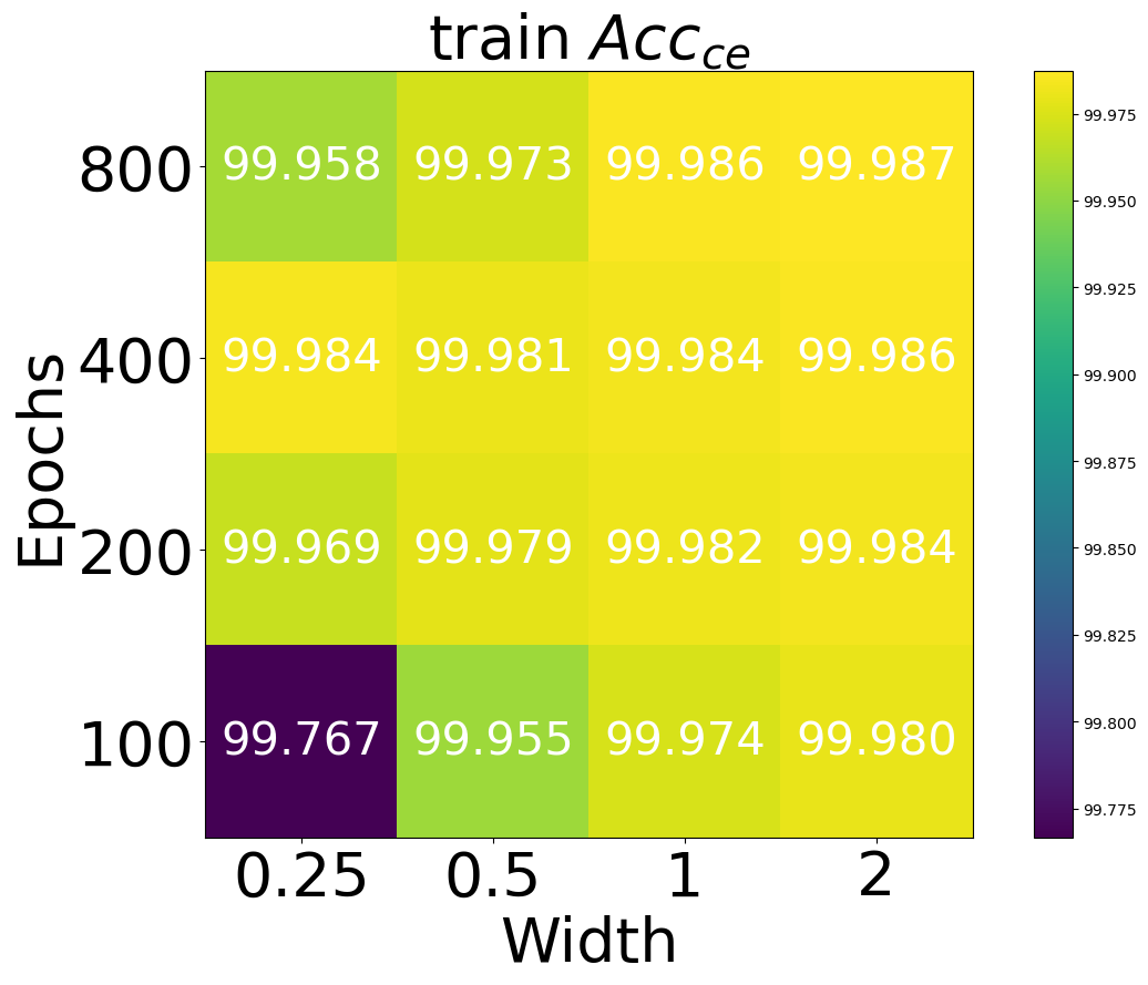
(a)

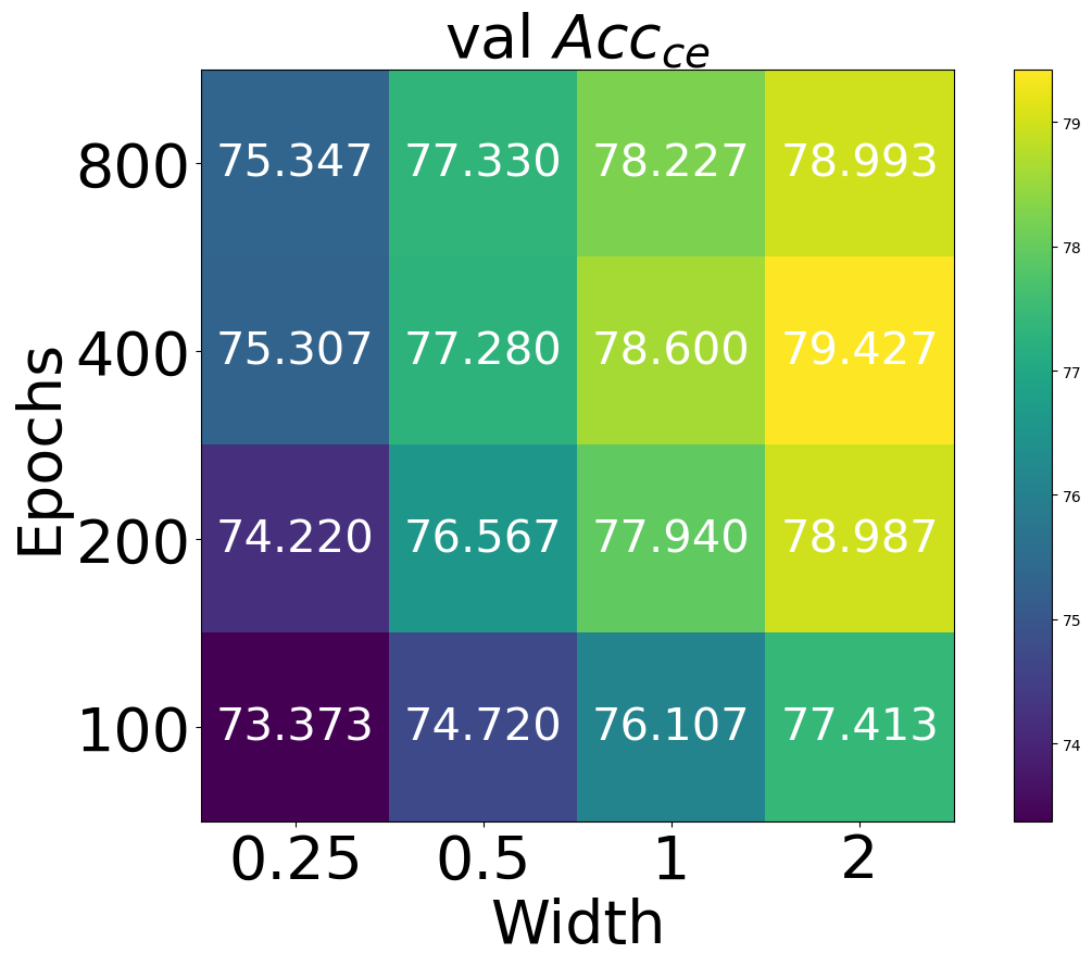
(b)

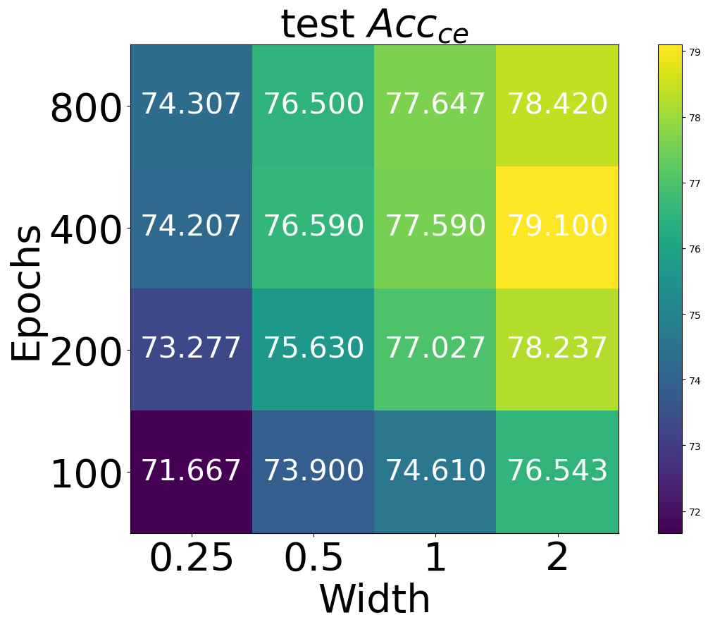
(c)

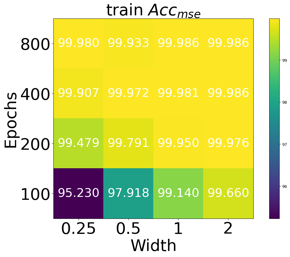
(d)

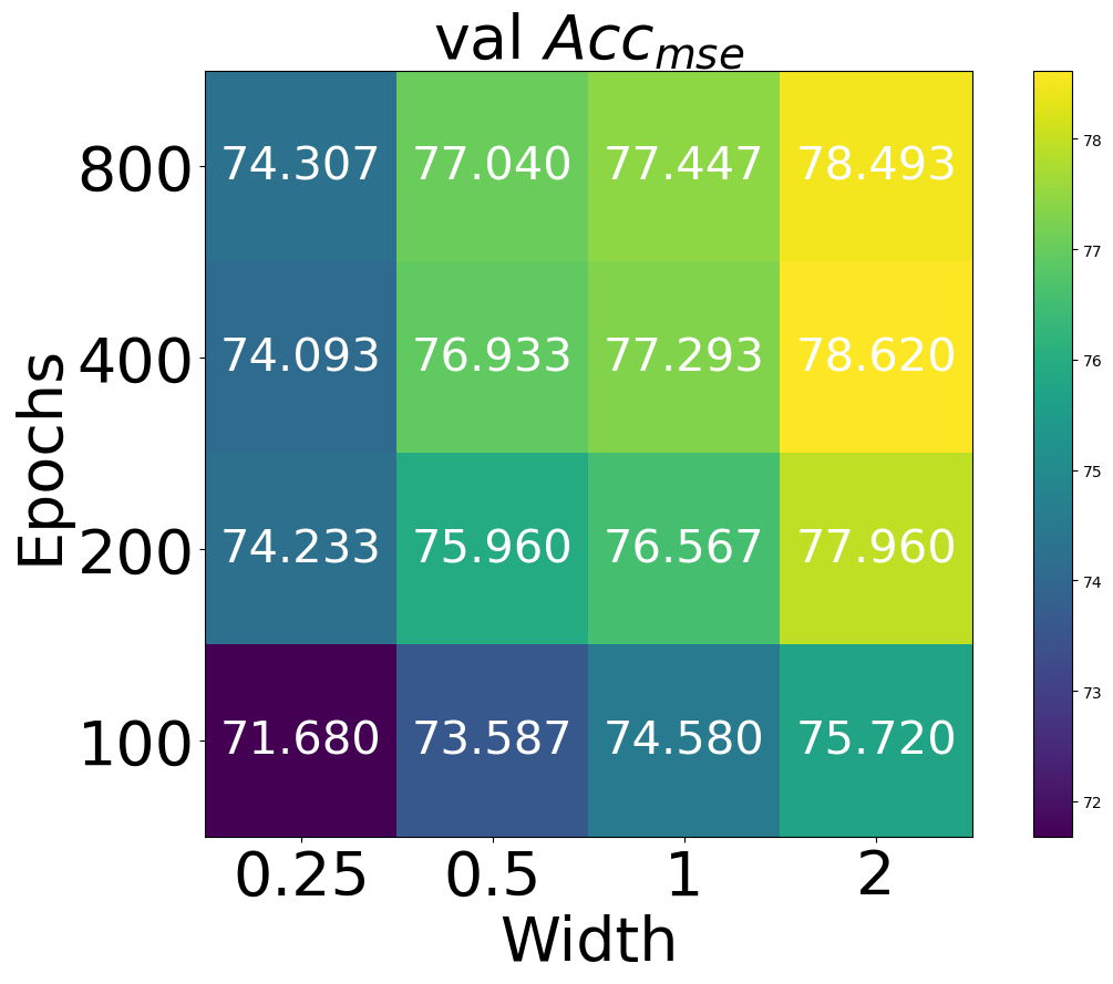
(e)

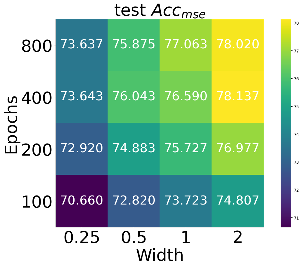
(f)

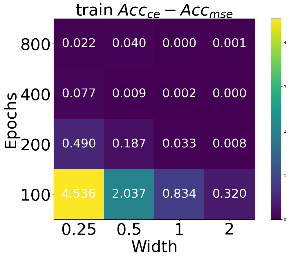
(g)

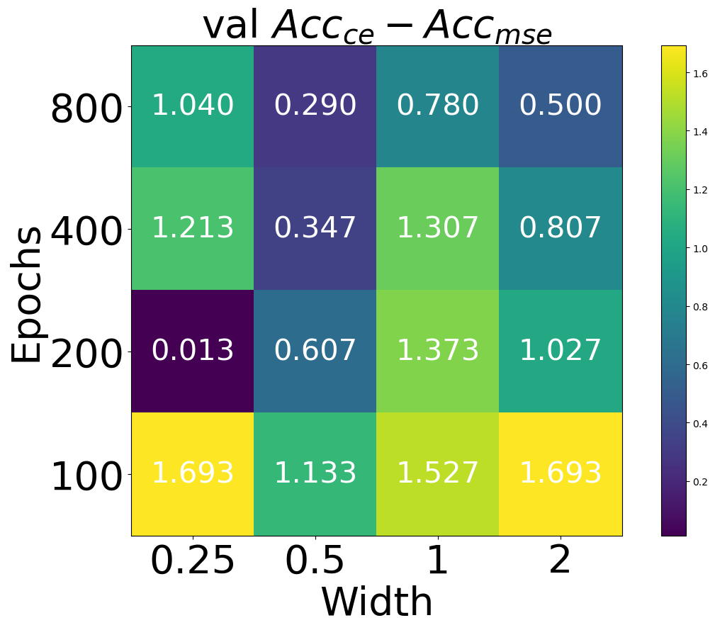
(h)

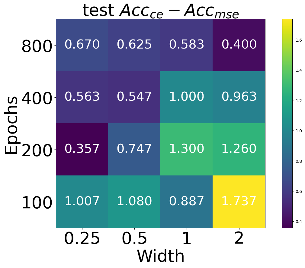
(i)

Figure 1: Illustration of $\text{Acc}_{CE}-\text{Acc}_{l},l\in[\text{fl, ls,mse}]$  across different losses with step-decay learning rate schedule and WideResNet50 with different training epochs and width.

Organizations and Basic.

The appendix is organized as follows. We first introduce the basic definitions and inequalities used throughout the appendices. In Section 2, we provide more details about the datasets, computational resources, and more experiment results on CIFAR10, CIFAR100 and miniImageNet datasets. In Section 3, we prove that CE, FL and LS satisfy the contrastive property in LABEL:def:GLoss. In Section 4, we provide a detailed proof for LABEL:thm:global-minima, showing that the Simplex ETFs are the only global minimizers, as long as the loss function satisfies the LABEL:def:GLoss. Finally, in Appendix 5, we present the whole proof for LABEL:thm:global-geometry that the FL function is a locally strict saddle function with no spurious local minimizers existing locally and LS function is a globally strict saddle function with no spurious local minimizers existing globally.

[$K$-Simplex ETF] A standard Simplex ETF is a collection of points in $\mathbb{R}^{K}$ specified by the columns of

$$\mathbf{M}\;=\;\sqrt{\frac{K}{K-1}}\left(\mathbf{I}_{K}-\frac{1}{K}\mathbf{1}_{K}\mathbf{1}_{K}^{\top}\right),$$

where $\mathbf{I}_{K}\in\mathbb{R}^{K\times K}$ is the identity matrix, and $\mathbf{1}_{K}\in\mathbb{R}^{K}$ is the all ones vector. In the other words, we also have

$$\mathbf{M}^{\top}\mathbf{M}\;=\;\mathbf{M}\mathbf{M}^{\top}\;=\;\frac{K}{K-1}\left(\mathbf{I}_{K}-\frac{1}{K}\mathbf{1}_{K}\mathbf{1}_{K}^{\top}\right).$$

As in [papyan2020prevalence, fang2021layer], in this paper we consider general Simplex ETF as a collection of points in $\mathbb{R}^{d}$ specified by the columns of $\sqrt{\frac{K}{K-1}}\bm{P}\left(\mathbf{I}_{K}-\frac{1}{K}\mathbf{1}_{K}\mathbf{1}_{K}^{\top}\right)$, where $\bm{P}\in\mathbb{R}^{d\times K}(d\geq K)$ is an orthonormal matrix, i.e., $\bm{P}^{\top}\bm{P}=\mathbf{I}_{K}$.

[Young’s Inequality] Let $p,q$ be positive real numbers satisfying $\frac{1}{p}+\frac{1}{q}=1$. Then for any $a,b\in\mathbb{R}$, we have

$$\left|ab\right|\;\leq\;\frac{\left|a\right|^{p}}{p}\;+\;\frac{\left|b\right|^{q}}{q},$$

where the equality holds if and only if $\left|a\right|^{p}=\left|b\right|^{q}$. The case $p=q=2$ is just the AM-GM inequality for $a^{2},\;b^{2}$: $\left|ab\right|\leq\frac{1}{2}\left(a^{2}+b^{2}\right)$, where the equality holds if and only if $\left|a\right|=\left|b\right|$.

The following Lemma extends the standard variational form of the nuclear norm. For any fixed $\bm{W}\in\mathbb{R}^{K\times d}$, $\bm{H}_{i}\in\mathbb{R}^{d\times K}$, $\bar{\bm{Z}}_{i}=\bm{W}\bm{H}_{i}\in\mathbb{R}^{K\times K}$ and $\alpha>0$, we have

$$\left\|\bar{\bm{Z}}_{i}\right\|_{*}\;\leq\;\frac{1}{2\sqrt{\alpha}}\left(\left\|\mathbf{W}\right\|_{F}^{2}+\alpha\left\|\mathbf{H}_{i}\right\|_{F}^{2}\right).$$ (1)

Here, $\left\|\bar{\bm{Z}}_{i}\right\|_{*}$ denotes the nuclear norm of $\bar{\bm{Z}}_{i}$:

$$\left\|\bar{\bm{Z}}_{i}\right\|_{*}\;:=\;\sum_{k=1}^{K}\sigma_{k}(\bar{\bm{Z}}_{i})=\operatorname{trace}\left(\mathbf{\Sigma}\right),\quad\text{with}\quad\bar{\bm{Z}}_{i}\;=\;\mathbf{U}\mathbf{\Sigma}\mathbf{V}^{\top},$$

where $\left\{\sigma_{k}\right\}_{k=1}^{K}$ denotes the singular values of $\bar{\bm{Z}}_{i}$, and $\bar{\bm{Z}}_{i}=\mathbf{U}\mathbf{\Sigma}\mathbf{V}^{\top}$ is the singular value decomposition (SVD) of $\bar{\bm{Z}}_{i}$.

Proof [Proof of Lemma 1.2] Let $\bar{\bm{Z}}_{i}=\mathbf{U}\mathbf{\Sigma}\mathbf{V}^{\top}$ be the SVD of $\bar{\bm{Z}}_{i}$. For any $\mathbf{W}\mathbf{H}_{i}=\bar{\bm{Z}}_{i}$, we have

$$\left\|\bar{\bm{Z}}_{i}\right\|_{*}\; =\;\operatorname{trace}\left(\mathbf{\Sigma}\right)\;=\;\operatorname{trace}\left(\mathbf{U}^{\top}\bar{\bm{Z}}_{i}\mathbf{V}\right)\;=\;\operatorname{trace}\left(\mathbf{U}^{\top}\mathbf{W}\mathbf{H}_{i}\mathbf{V}\right)$$

$$\leq\;\frac{1}{2\sqrt{\alpha}}\left\|\mathbf{U}^{\top}\mathbf{W}\right\|_{F}^{2}+\frac{\sqrt{\alpha}}{2}\left\|\mathbf{H}_{i}\mathbf{V}\right\|_{F}^{2}\;\leq\;\frac{1}{2\sqrt{\alpha}}\left(\left\|\mathbf{W}\right\|_{F}^{2}+\alpha\left\|\mathbf{H}_{i}\right\|_{F}^{2}\right),$$

where the first inequality utilize the Young’s inequality in Lemma 1.2 that $\left|\operatorname{trace}(\bm{A}\bm{B})\right|\leq\frac{1}{2c}\left\|\bm{A}\right\|_{F}^{2}+\frac{c}{2}\left\|\bm{B}\right\|_{F}^{2}$ for any $c>0$ and $\bm{A},\bm{B}$ of appropriate dimensions, and the last inequality follows because $\left\|\mathbf{U}\right\|=1$ and $\left\|\mathbf{V}\right\|=1$. Therefore, we have

$$\left\|\bar{\bm{Z}}_{i}\right\|_{*}\;\leq\;\frac{1}{2\sqrt{\alpha}}\left(\left\|\mathbf{W}\right\|_{F}^{2}+\alpha\left\|\mathbf{H}_{i}\right\|_{F}^{2}\right).$$

We complete the proof.  

[Eigenvalues of Diagonal-Plus-Rank-One Matrices] Let $\tau<0$, $\bm{z}\in\mathbb{R}^{n}$, and $\bm{D}$ be an $n\times n$ diagonal matrix with diagonals $d_{1},\ldots,d_{n}$. Let $\lambda_{1},\ldots,\lambda_{n}$ be the eigenvalues of the diagonal-plus-rank-one matrix $\bm{D}+\tau\bm{z}\bm{z}^{\top}$.

• Case 1: If $d_{1}>d_{2}>\cdots>d_{n}$ and $z_{i}\neq 0$ for all $i=1,\cdots,n$, then the eigenvalues $\{\lambda_{i}\}$ are equal to the $n$ roots of the rational function [cuppen1980divide, stor2015forward]

  $$w(\lambda)=1+\tau\bm{z}^{\top}\left(\bm{D}-\lambda\mathbf{I}\right)^{-1}\bm{z}=1+\tau\sum_{j=1}^{n}\frac{z_{j}^{2}}{d_{j}-\lambda},$$

  and the diagonals $\{d_{i}\}$ strictly separate the eigenvalues as following:

  $$d_{1}>\lambda_{1}>d_{2}>\lambda_{2}>\cdots>d_{n}>\lambda_{n}.$$ (2)

• Case 2:If $z_{i}=0$ for some $i$, then $d_{i}$ is an eigenvalue of $\bm{D}+\tau\bm{z}\bm{z}^{\top}$ with corresponding eigenvector $\bm{e}_{i}$ since

  $$(\mathbf{D}+\tau\bm{z}\bm{z}^{\top})\bm{e}_{i}=d_{i}\bm{e}_{i}+\tau\bm{z}z_{i}=d_{i}\bm{e}_{i}.$$

  The remaining $n-1$ eigenvalues of $\bm{D}+\tau\bm{z}\bm{z}^{\top}$ are equal to the eigenvalues of the smaller matrix $\bm{D}^{\prime}+\tau\bm{z}^{\prime}\bm{z}^{{}^{\prime}\top}$, where $\bm{D}^{\prime}\in\mathbb{R}^{(n-1)\times(n-1)}$ and $\bm{z}^{\prime}\in\mathbb{R}^{n-1}$ are obtained by removing the $i$-th rows and columns from $\bm{D}$ and the $i$-th element from $\bm{z}$, respectively. One can repeat this process if $\bm{z}^{\prime}$ still has zero element.

• Case 3: If there are $m$ mutually equal diagonal elements, say $d_{i+1}=\cdots=d_{i+m}=d$, then for any orthogonal $m\times m$ matrix $\bm{P}$, $\bm{D}+\tau\bm{z}\bm{z}^{\top}$ has the same eigenvalues as

  $$\bm{T}\bm{D}\bm{T}^{\top}+\tau(\bm{T}\bm{z})(\bm{T}\bm{z})^{\top}=\bm{D}+\tau\widehat{\bm{z}}\widehat{\bm{z}}^{\top},\ \text{where}\ \bm{T}=\begin{bmatrix}\mathbf{I}_{i}&&\\ &\bm{P}&\\ &&\mathbf{I}_{n-i-m}\end{bmatrix},\widehat{\bm{z}}=\bm{T}\widehat{\bm{z}}.$$

  We can then choose $\bm{P}$ as a Householder transformation such that

  $$\bm{P}\begin{bmatrix}z_{i+1}&z_{i+2}&\cdots&z_{i+m}\end{bmatrix}^{\top}=\begin{bmatrix}0&0&\cdots&\sqrt{\sum_{j=i+1}^{i+m}z_{j}^{2}}\end{bmatrix}^{\top}.$$

  Thus, according to Case 2, $d$ is an eigenvalue of $\bm{D}+\tau\widehat{\bm{z}}\widehat{\bm{z}}^{\top}$ repeated $m-1$ times and the remaining eigenvalues can be computed by checking the smaller matrix.

Based on Section 1.2, we can prove the following Lemma.

Let $K\geq 3$ and $\bm{Z}=-\left(\mathbf{I}_{K}-\frac{1}{K}\bm{1}\bm{1}^{\top}\right)\text{diag}\left(\rho_{1},\rho_{2},\cdots,\rho_{K}\right)$ with $|\rho_{1}|\geq|\rho_{2}|\geq\cdots\geq|\rho_{K}|$ and $|\rho_{1}|>0$. Also let $\sigma_{i}\geq 0$ be the $i$-th largest singular value of $\bm{Z}$. Suppose there exists $k$ with $1\leq k\leq K-1$ such that

$$\sigma_{1}=\cdots=\sigma_{k}=\sigma_{\max}>0\ \text{and}\ \sigma_{k+1}=\cdots=\sigma_{K}=0.$$ (3)

Then $|\rho_{1}|,\cdots,|\rho_{K}|$ must satisfy either

$$|\rho_{1}|=|\rho_{2}|=\cdots=|\rho_{K}|,\quad\text{with}\quad\sigma_{\max}=|\rho_{1}|,$$

or

$$\rho_{2}=\cdots=\rho_{K}=0,\quad\text{with}\quad\sigma_{\max}=\sqrt{\frac{K-1}{K}}|\rho_{1}|.$$

Proof [Proof of Lemma 1.2] Because

$$\bm{Z}^{\top}\bm{Z} =\text{diag}\left(\rho_{1},\rho_{2},\cdots,\rho_{K}\right)\left(\mathbf{I}_{K}-\frac{1}{K}\bm{1}\bm{1}^{\top}\right)\text{diag}\left(\rho_{1},\rho_{2},\cdots,\rho_{K}\right)$$

$$=\text{diag}\left(\rho_{1}^{2},\rho_{2}^{2},\cdots,\rho_{K}^{2}\right)-\frac{1}{K}\mathbf{\rho}\mathbf{\rho}^{\top}$$

where $\mathbf{\rho}=\begin{bmatrix}\rho_{1}&\rho_{2}&\cdots&\rho_{K}\end{bmatrix}^{\top}$, $\bm{Z}^{\top}\bm{Z}$ satisfies the form of Diagonal-Plus-Rank-One in Section 1.2 with $\mathbf{D}=\text{diag}\left(\rho_{1}^{2},\rho_{2}^{2},\cdots,\rho_{K}^{2}\right)$, $\bm{z}=\mathbf{\rho}$ and $\tau=-\frac{1}{K}$. Let $\lambda_{1}\geq\lambda_{2}\geq\cdots\lambda_{K}\geq 0$ denote the $n$ eigenvalues of $\bm{Z}^{\top}\bm{Z}$. Due to $\bm{1}^{\top}\bm{Z}=\bm{0}^{\top}$, we can have $\lambda_{K}=0$.

• If $|\rho_{1}|=|\rho_{2}|=\cdots=|\rho_{K}|$: we have

  $$\rho_{1}^{2}=\lambda_{1}=\cdots=\lambda_{K-1}=\rho_{K}^{2}>\lambda_{K}=0.$$

  Thus, $\sigma_{\max}=\sqrt{\lambda_{1}}=|\rho_{1}|$.

• If $|\rho_{1}|>|\rho_{2}|=\cdots=|\rho_{K}|=0$: according to Case 2 in Section 1.2, we have

  $$\lambda_{1}=\left(1-1/K\right)\rho_{1}^{2}>\rho_{2}^{2}=\lambda_{2}\cdots=\rho_{K}^{2}=\lambda_{K}=0.$$

  Thus, $\sigma_{\max}=\sqrt{\left(1-1/K\right)\rho_{1}^{2}}=\sqrt{{(K-1)}/{K}}|\rho_{1}|$.

• If $|\rho_{1}|>|\rho_{2}|=\cdots=|\rho_{K}|\neq 0$: according to Case 3 in Section 1.2, we have

  $$\lambda_{2}\cdots=\lambda_{K-1}=\rho_{2}^{2}$$

  and the remaining two eigenvalues are the same to those of $\begin{bmatrix}\rho_{1}^{2}&\\ &\rho_{K}^{2}\end{bmatrix}+(-\frac{1}{K})\begin{bmatrix}\rho_{1}\\ \sqrt{K-1}\rho_{K}\end{bmatrix}\begin{bmatrix}\rho_{1}&\sqrt{K-1}\rho_{K}\end{bmatrix}$. According to (2) in Section 1.2, we can obtain

  $$\rho_{1}^{2}>\lambda_{1}>\rho_{K}^{2}>\lambda_{K}=0.$$

  Combing them together, we can have

  $$\rho_{1}^{2}>\lambda_{1}>\rho_{2}^{2}=\lambda_{2}\cdots=\rho_{K}^{2}>\lambda_{K}=0$$

  thus, $0=\lambda_{K}<\lambda_{2}<\lambda_{1}=\lambda_{\max}$, which violates the assumption (3).

• If $|\rho_{1}|=\cdots=|\rho_{i}|>|\rho_{i+1}|=\cdots=|\rho_{K}|=0$ and $1<i<K$: according to the Case 2 and Case 3 in Section 1.2, we can have

  $$\lambda_{1}=\cdots=\lambda_{i-1}=\rho_{1}^{2}$$

  $$\lambda_{i+1}=\cdots=\lambda_{K}=0$$

  and $0<\lambda_{i}=\rho_{1}^{2}-\frac{i}{K}\rho_{1}^{2}<\rho_{1}^{2}=\lambda_{\max}$, which violates the assumption (3).

• If $|\rho_{1}|=\cdots=|\rho_{i}|>|\rho_{i+1}|=\cdots=|\rho_{K}|\neq 0$ and $1<i<K$: according to Case 3 in Section 1.2, we have

  $$\lambda_{1}=\cdots=\lambda_{i-1}=\rho_{1}^{2}$$

  $$\lambda_{i+1}=\cdots=\lambda_{K-1}=\rho_{K}^{2}$$

  and the remaining two eigenvalues are the same to those of $\bm{D}=\begin{bmatrix}\rho_{1}^{2}&\\ &\rho_{K}^{2}\end{bmatrix}+(-\frac{1}{K})\begin{bmatrix}\sqrt{i}\rho_{1}\\ \sqrt{K-i}\rho_{K}\end{bmatrix}\begin{bmatrix}\sqrt{i}\rho_{1}&\sqrt{K-i}\rho_{K}\end{bmatrix}$. According to (2) in Section 1.2, we can obtain

  $$\rho_{1}^{2}=\rho_{i}^{2}>\lambda_{i}>\rho_{K}^{2}>\lambda_{K}=0.$$

  Combing them together, we can have

  $$\rho_{1}^{2}=\lambda_{1}=\cdots=\rho_{i}^{2}>\lambda_{i}>\rho_{i+1}^{2}=\lambda_{i+1}=\cdots=\rho_{K}^{2}>\lambda_{K}=0$$

  thus, $0=\lambda_{K}<\lambda_{i}<\lambda_{1}=\lambda_{\max}$, which violates the assumption (3).

• If $|\rho_{1}|>|\rho_{i}|>|\rho_{K}|$ for some $1<i<K$: Suppose $|\rho_{1}|=\cdots=|\rho_{m}|$, $|\rho_{i}|=\cdots=|\rho_{i+n-1}|$ and $|\rho_{K-t+1}|=\cdots=|\rho_{K}|$, where $m<i$, $i+n-1<K-t+1$ and $m,n,t\geq 1$. According to the (2), Case 2 and Case 3 in Section 1.2, we can find

  $$\rho_{m}^{2}>\lambda_{m}>\rho_{i}^{2}\geq\lambda_{i+n-1}>\rho_{K}^{2}\geq\lambda_{K}=0$$

  thus, $0=\lambda_{K}<\lambda_{i+n-1}<\lambda_{m}\leq\lambda_{\max}$, which violates the assumption (3).

We complete the proof.  

2 Experiments

In this section, we first describe more details about the datasets and the computational resource used in the paper. Particularly, all CIFAR10, CIFAR100 and miniImageNet are publicly available for academic purpose under the MIT license, and we run all experiments on a single RTX3090 GPU with 24GB memory. Moreover, additional experimental results on CIFAR10, CIFAR100 and miniImageNet are presented in Section 2.1, Section 2.2, and Section 2.3, respectively.

2.1 Additional experimental results on CIFAR10

In LABEL:sec:experiment, we present the test accuracy for different losses function across various different iteration-width configurations. Moreover, we further show the ${\mathcal{N}C}_{1}$ for different loss functions across different iteration-width configurations , and we reuse the results of test accuracy in LABEL:fig:lossmap-cifar10 for better investigation. The experiment results in Figure 2 consistently show that the value of ${\mathcal{N}C}_{1}$ of training WideResNet50-0.25 for 100 epochs is around three orders of magnitude larger than it of training WideResNet50-2 for 800 epochs, which indicates that the previous configuration setting is much less collapsed than the latter one. In terms of test accuracy, the maximal difference across different losses for $\text{width}=0.25$ and $\text{epochs}=100$ configuration is $1.037\%$, which is larger than $0.36\%$ for $\text{width}=2$ and $\text{epochs}=800$ configuration. These results support our claim that all losses lead to identical performance, as long as the network has sufficient approximation power and the number of optimization is enough for the convergence to the $\mathcal{NC}$ global optimality.

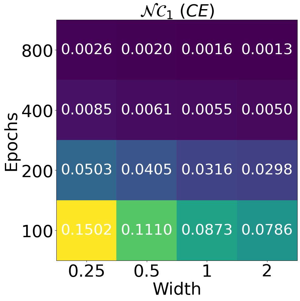
(a)

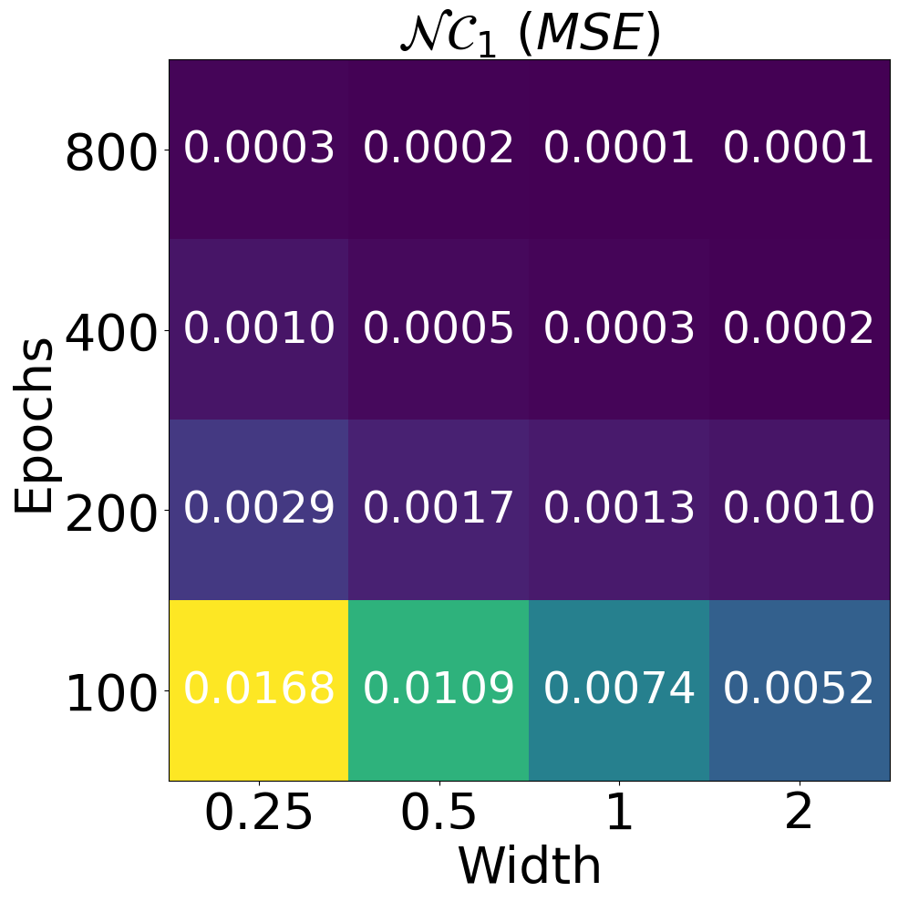
(b)

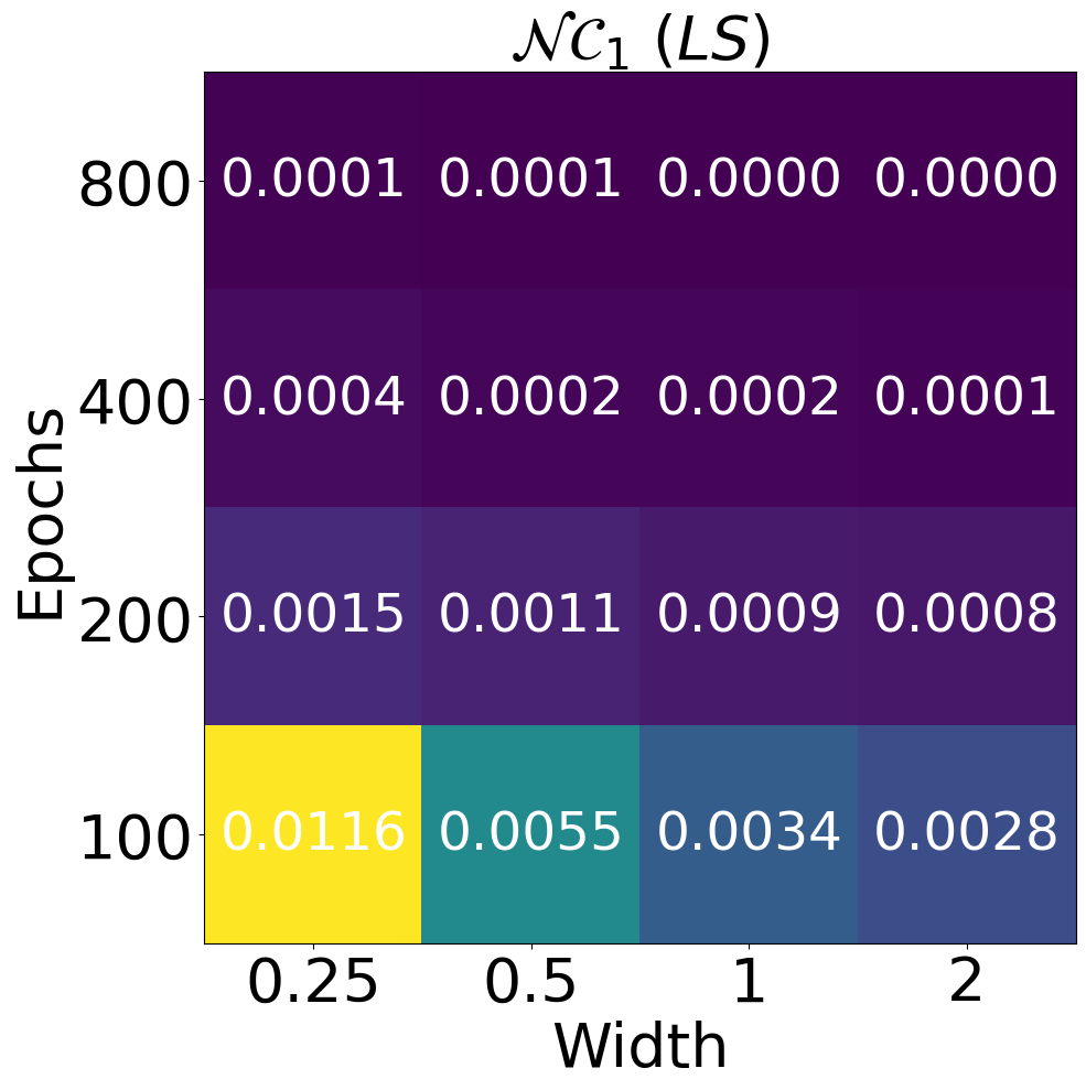
(c)

(d)

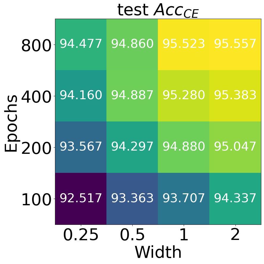
(e)

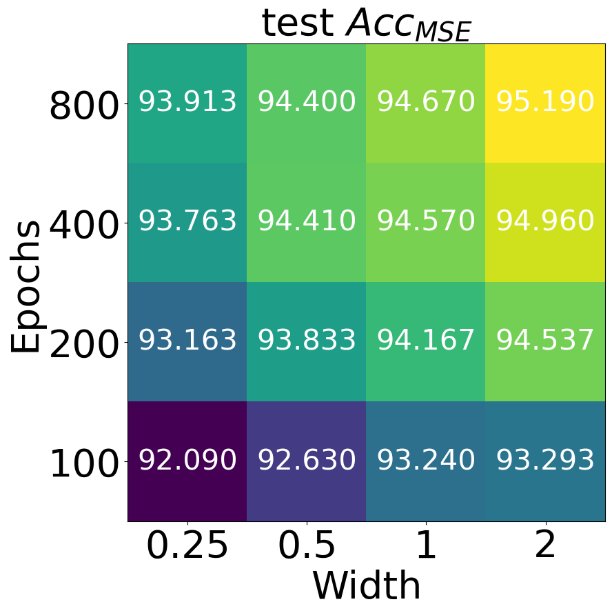
(f)

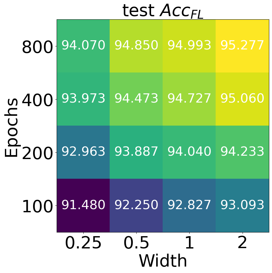
(g)

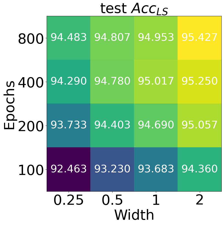
(h)

Figure 2: Illustration of ${\mathcal{N}C}_{1}$ and test accuracy across different iterations-width configurations. The figure depicts the ${\mathcal{N}C}_{1}$ and test accuracy of various iteration-width configurations for different loss functions on CIFAR10.

2.2 Additional experimental results on CIFAR100

In this parts, we show the additional results on CIFAR100 dataset.

Prevalence of $\mathcal{NC}$ Across Varying Training Losses

We show that all loss functions lead to $\mathcal{NC}$ solutions during the terminal phase of training on CIFAR100 dataset. The results on CIFAR100 using WideResNet50-2 and different loss functions is provided in Figure 3. We consistently observe that all three $\mathcal{NC}$ metrics of FL and MSE converge to a small value as training progresses, and metrics of CE and FL still continue to decrease at the last iteration, because CIFAR100 is more difficult than CIFAR10 and requires networks to be optimized longer. The decreasing speed of FL is slowest, which is consistent with our global landscape analysis that FL has benign landscape in the local region near optimality. These results imply that all losses exhibit $\mathcal{NC}$ at the end, regardless of the choice of loss functions.

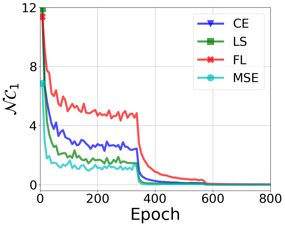
(a)

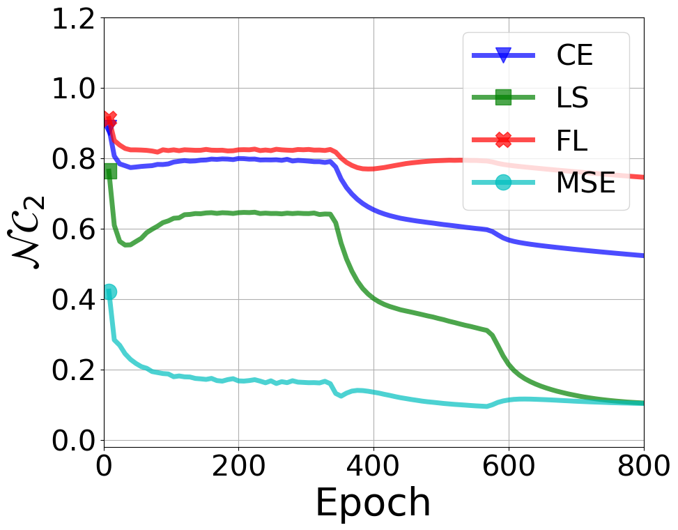
(b)

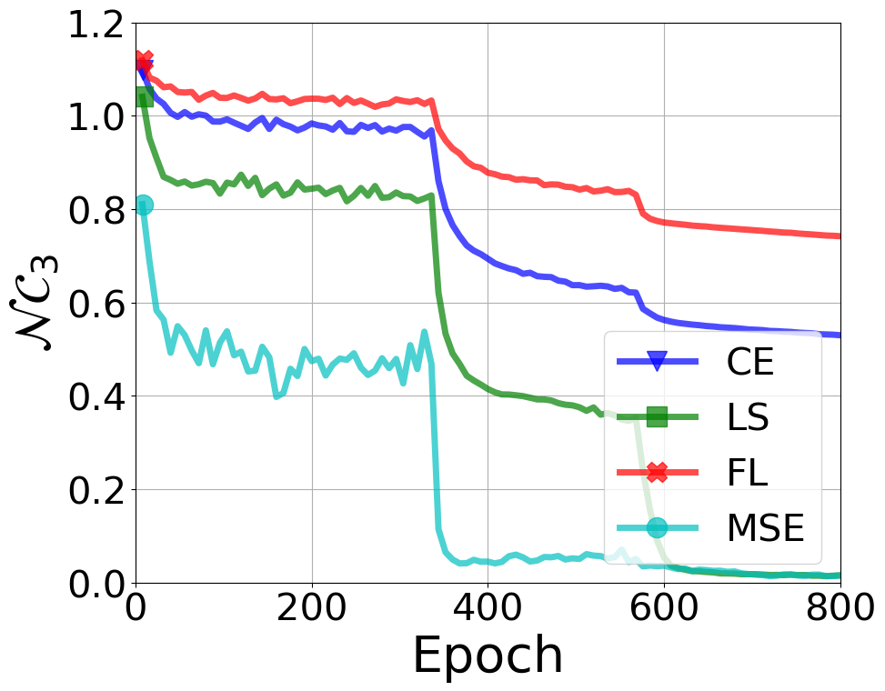
(c)

Figure 3: The evolution of $\mathcal{NC}$ metrics across different loss functions. We train the WideResNet50-2 on CIFAR100 dataset for 800 epochs using different loss function. From left to right: $NC_{1}$ (variability collapse), $NC_{2}$ (convergence to simplex ETF) and $NC_{3}$ (convergence to self-duality).

All Losses Lead to Largely Identical Performance

Same as the results on CIFAR10 dataset, the conclusion on CIFAR100 also holds that all loss functions have largely identical performance once the training procedure converges to the $\mathcal{NC}$ global optimality. In Figure 4, we plot the evolution of the training accuracy, validation accuracy and test accuracy with training progressing, where all losses are optimized on the same WideResNet50-2 architecture and CIFAR100 for 800 epochs. To reduce the randomness, we average the results from 3 different random seeds per iteration-width configuration, and the test accuracy is reported based on the model with best accuracy on validation set, where we organize the validation set by holding out 10 percent data from the training set. The results consistently shows that the training accuracy trained by different losses all converge to one hundred percent (reaching to terminal phase), and the validation accuracy and test accuracy across different losses are largely same, as long as the optimization procedure converges to the $\mathcal{NC}$ global solution. In Figure 5, we plot the average ${\mathcal{N}C}_{1}$ and test accuracy of different losses under different pairs of width and iterations for CIFAR100 dataset. The three phenomenon mentioned in LABEL:exp:same-performance-across-losses also exist on CIFAR100 in most cases. Moreover, the values of ${\mathcal{N}C}_{1}$ for width=0.25 and epochs=100 configuration are also around three orders magnitude larger than them for width=2 and epochs=800 configuration and the less collapsed configuration leads to larger difference gap across different loss functions. While there are some small difference between different losses in $\text{width}=2$ and $\text{epochs}=800$ configurations, We guess that it is because CIFAR100 is much harder than CIFAR10 datasets, and network is not sufficiently large and trained not long enough for all losses to achieve a global solution.

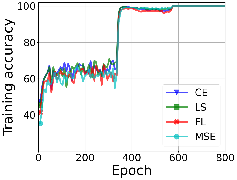
(a)

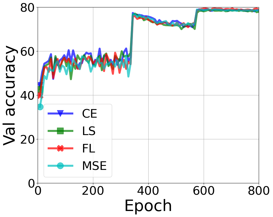
(b)

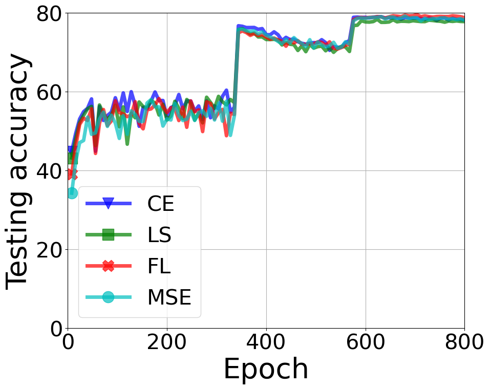
(c)

Figure 4: The evolution of performance across different loss functions. We train the WideResNet50-2 on CIFAR100 dataset for 800 epochs using different loss function. From left to right: training accuracy, validation accuracy and test accuracy.

(a)

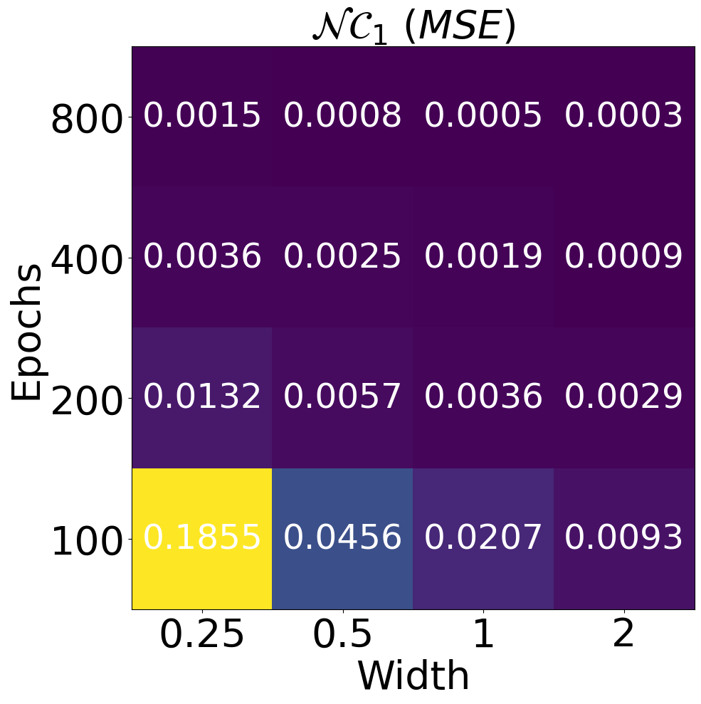
(b)

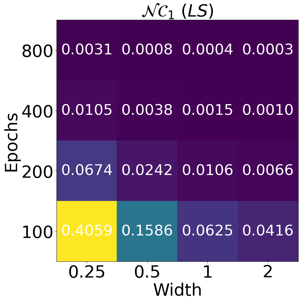
(c)

(d)

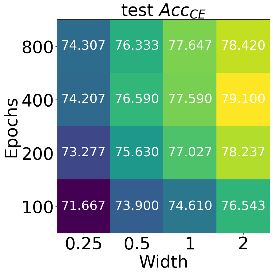
(e)

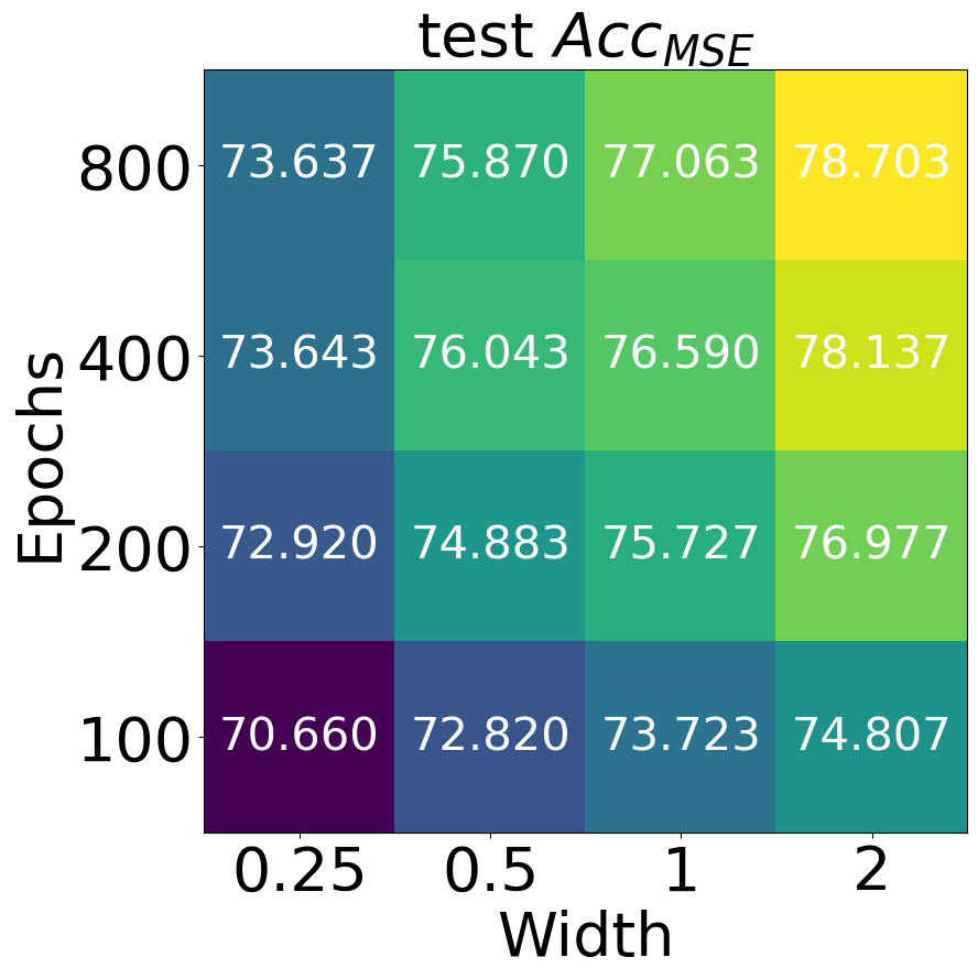
(f)

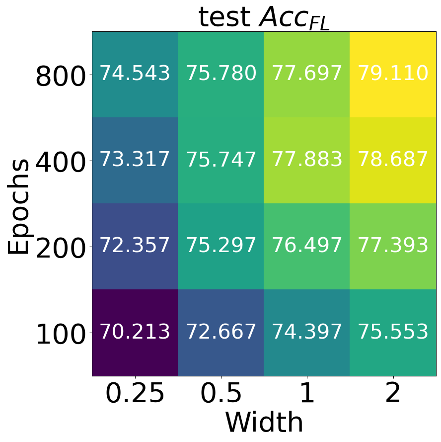
(g)

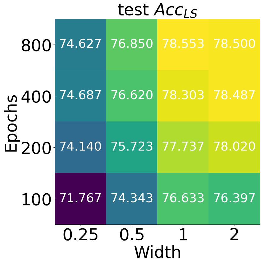
(h)

Figure 5: Illustration of ${\mathcal{N}C}_{1}$ and test accuracy across different iterations-width configurations. The figure depicts the ${\mathcal{N}C}_{1}$ and test accuracy of various iteration-width configurations for different loss functions on CIFAR100.

2.3 Additional experimental results on miniImageNet

In this parts, we show the additional results on miniImageNet dataset. We trained WideResNet18-0.25 and WideResNet18-2 on miniImageNet for 100 epochs and 800 epochs, respectively. To reduce the randomness, we average the results from 3 different random trials. The ${\mathcal{N}C}_{1}$ and test accuracy of different loss functions are provided in Figure 6 for comparison. We consistently observe that the ${\mathcal{N}C}_{1}$ metric of all losses converges to a small value as training progress, when the neural network has sufficient approximation power and the training is performed for sufficiently many iterations, such as WideResNet18-2 for 800 epochs. Additionally, the conclusion on miniImageNet also holds that all loss functions have largely identical performance once the training procedure converges to the $\mathcal{NC}$ global optimality. Specifically, while the last-iteration test accuracy of training WideResNet18-0.25 for 100 epochs is $0.7195$, $0.6915$, $0.7020$ and $0.7040$, respectively, the last-iteration test accuracy of training WideResNet18-2 for 800 epochs is $0.7930$, $0.7962$, $0.7932$ and $0.8020$ for CE, MSE, FL and LS, respectively. The experiment results on miniImageNet also support our claim that $(i)$ the test performance may be different across different loss functions when the network is not large enough and is optimized with limited number of iterations, but $(ii)$ the test accuracy across different loss are largely identical, once the networks has sufficient capacity and the training is optimized to converge to the $\mathcal{NC}$ global solution.

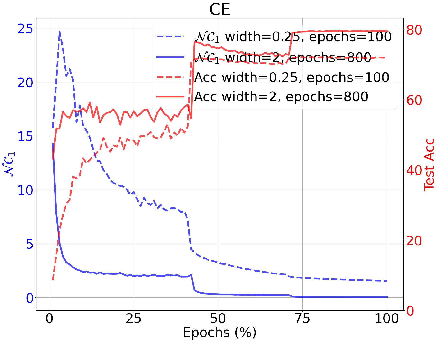
(a)

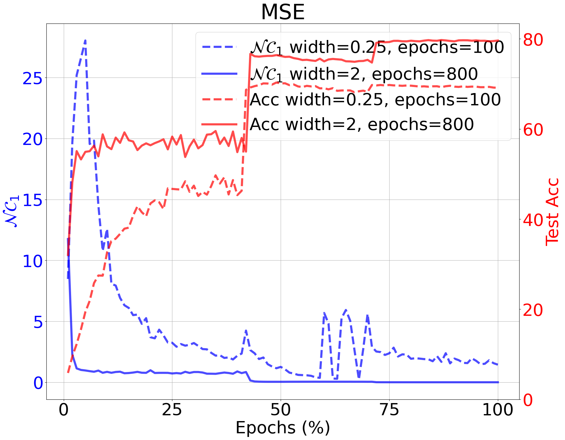
(b)

(c)

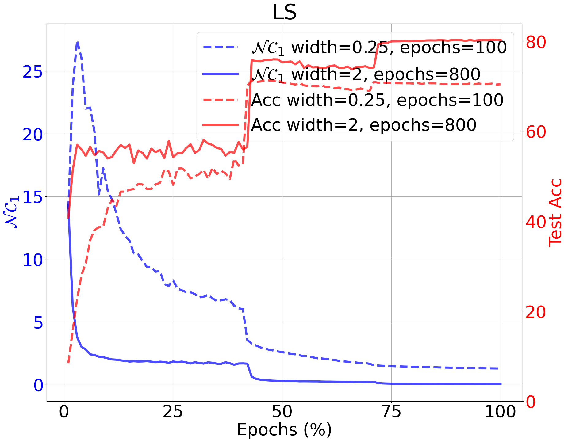
(d)

Figure 6: The evolution of ${\mathcal{N}C}_{1}$ and test accuracy across different loss functions. We train the WideResNet18-0.25 for 100 epochs and WideResNet18-2 for 800 epochs on miniImageNet using different loss functions.

3 Proof of CE, FL and LS included in GL

In this section, we prove that CE, FL and LS belong to GL in Section 3.1, Section 3.2 and Section 3.3, respectively. Before starting the proof for each loss, let us restate the definition of the GL in LABEL:def:GLoss:

[Contrastive property] We say a loss function $\Lgl(\bm{z},\bm{y}_{k})$ satisfies the contrastive property if there exists a function $\phi$ such that $\Lgl(\bm{z},\bm{y}_{k})$ can be lower bounded by

$$\Lgl(\bm{z},\bm{y}_{k})\geq\phi\left(\sum_{j\neq k}(z_{j}-z_{k})\right)$$ (4)

where the equality holds only when $z_{j}=z_{j}^{\prime}$ for all $j,j^{\prime}\neq k$. Moreover, $\phi(t)$ satisfies

$$t^{*} =\arg\min_{t}\phi\left(t\right)+c|t|\text{ is unique for any }c>0,\text{and }t^{*}\leq 0.$$ (5)

3.1 CE is in GL

In this section, we will show that the CE defined in (LABEL:def:ce) belongs to the GL defined in Section 3. First, let us rewrite the CE definition in GL form as following:

$$\mathcal{L}_{\mathrm{CE}}(\bm{z},\bm{y}_{k})\; =\;-\log\left(\frac{\exp(z_{k})}{\sum_{j=1}^{K}\exp(z_{j})}\right)\;=\;\log\left(1+\sum_{j\neq k}^{K}\exp(z_{j}-z_{k})\right)$$

$$\geq\;\log\left(1+(K-1)\exp{\left(\frac{z_{j}-z_{k}}{K-1}\right)}\right)=\phi_{\text{CE}}\left(\sum_{j\neq k}(z_{j}-z_{k})\right).$$

where the inequality is due to the $\log$ is an increasing and function and $\exp$ is a strictly convex function, and it achieves equality only when $z_{j}=z_{j^{\prime}}$ for all $j,j^{\prime}\neq k$. Therefore, there exists such a function $\phi_{\text{CE}}$ to lower bound original CE loss $\mathcal{L}_{\mathrm{CE}}(\bm{z},\bm{y}_{k})$ as following:

$$\phi_{\text{CE}}(t)\; =\;\log\left(1+(K-1)\exp{\left(\frac{t}{K-1}\right)}\right),$$

which satisfies the condition of (4). Next, we will show $\phi_{\text{CE}}(t)$ satisfies the condition (5). The first-order gradient of $\phi_{\text{CE}}(t)$ is following:

$$\nabla\phi_{\text{CE}}(t) =\frac{\exp{\left(\frac{t}{K-1}\right)}}{1+(K-1)\exp{\left(\frac{t}{K-1}\right)}}$$

which is an increasing function and greater than $0$ for $t\in\mathbb{R}$. Let denote $\psi_{\text{CE}}(t)=\phi_{\text{CE}}(t)+c|t|$, then

• When $t\geq 0$: $\nabla\psi_{\text{CE}}(t)=\nabla\phi_{\text{CE}}(t)+c>0$, thus the $\psi_{\text{CE}}(t)$ is an increasing function w.r.t. $t$, and the minimizer is achieved when $t=0$.

• When $t\leq 0$: $\nabla\psi_{\text{CE}}(t)=\nabla\phi_{\text{CE}}(t)-c$, and $\nabla\phi_{\text{CE}}(t)$ is an increasing function, which achieves minimizer when $t=0$ such that $\nabla\phi_{\text{CE}}(t)=\frac{1}{K}$.

  • if $c\geq\frac{1}{K}$, $\nabla\psi_{\text{CE}}(t)<0$, and $\psi(t)$ is a decreasing function for $t\leq 0$, and the minimizer is achieved when $t=0$;

  • if $0<c\leq\frac{1}{K}$, there exist such $t^{*}$ such that $\nabla\psi_{\text{CE}}(t)=0$. When $t<t^{*}$, $\phi_{\text{CE}}(t)$ is a decreasing function; and when $t^{*}<t\leq 0$, $\phi_{\text{CE}}(t)$ is an increasing function. Therefore, the minimizer is achieved when $t=t^{*}<0$

Combing them together, we can prove that $\phi_{\text{CE}}$ satisfies the condition of (5).

3.2 FL is in GL

In this section, we will show that the FL defined in (LABEL:def:fl) belongs to the GL defined in Section 3. let us rewrite the FL definition in GL form as following:

$$\mathcal{L}_{\mathrm{FL}}(\bm{z},\bm{y}_{k})\; =\;-\left(1-\frac{\exp(z_{k})}{\sum_{j=1}^{K}\exp(z_{j})}\right)^{\gamma}\log\left(\frac{\exp(z_{k})}{\sum_{j=1}^{K}\exp(z_{j})}\right)$$

$$=\;\left(1-\frac{\exp(z_{k})}{\sum_{j=1}^{K}\exp(z_{j})}\right)^{\gamma}\log\left(\sum_{j=1}^{K}\exp(z_{j}-z_{k})\right)$$

$$=\;\left(1-\frac{1}{1+\sum_{j\neq k}^{K}\exp(z_{j}-z_{k})}\right)^{\gamma}\log\left(1+\sum_{j\neq k}^{K}\exp(z_{j}-z_{k})\right)$$

$$=\;\eta\left(1+\sum_{j\neq k}^{K}\exp(z_{j}-z_{k})\right)$$

where the function $\eta(t)=(1-\frac{1}{t})^{\gamma}\log\left(t\right)$ is an increasing function for $t\geq 1$ because

$$\nabla\eta(t) =\gamma(\frac{1}{t^{2}})(1-\frac{1}{t})^{\gamma-1}\log(t)+\frac{1}{t}(1-\frac{1}{t})^{\gamma}>0$$

Thus, we can find the lower bound function by

$$\mathcal{L}_{\mathrm{FL}}(\bm{z},\bm{y}_{k})\; \geq\;\eta\left(1+(K-1)\exp\left(\sum_{j\neq k}^{K}\frac{z_{j}-z_{k}}{K-1}\right)\right)$$

$$=\;\eta\left(\xi\left(\sum_{j\neq k}^{K}(z_{j}-z_{k})\right)\right)$$

$$=\;\phi_{\text{FL}}\left(\sum_{j\neq k}^{K}(z_{j}-z_{k})\right)$$

where $\phi_{\text{FL}}(t)=\eta\left(\xi\left(t\right)\right)$ and $\xi{\left(t\right)}=1+(K-1)\exp{\frac{t}{K-1}}\in[1,K]$, which satisfies the condition of (4). Next, we will show $\phi_{\text{FL}}(t)$ satisfies the condition (5). The first-order gradient of $\phi_{\text{FL}}(t)$ is following:

$$\nabla_{t}\psi_{\text{FL}}(t)\;=\;\nabla_{t}\left(\phi_{\text{FL}}(t)+c|t|\right)\;=\;\nabla_{\xi\left(t\right)}\eta\left(\xi\left(t\right)\right)\nabla_{t}{\xi\left(t\right)}+c\frac{t}{|t|}$$

$$\;=\; \left(\gamma\left(\frac{1}{\xi\left(t\right)}\right)^{2}\left(1-\frac{1}{\xi\left(t\right)}\right)^{\gamma-1}\log\left(\xi\left(t\right)\right)+\frac{1}{\xi\left(t\right)}\left(1-\frac{1}{\xi\left(t\right)}\right)^{\gamma}\right)\left(\exp{\left(\frac{t}{K-1}\right)}\right)+c\frac{t}{|t|}$$

$$\;=\; \left(\gamma\left(\frac{1}{\xi\left(t\right)}\right)^{2}\left(1-\frac{1}{\xi\left(t\right)}\right)^{\gamma-1}\log\left(\xi\left(t\right)\right)+\frac{1}{\xi\left(t\right)}\left(1-\frac{1}{\xi\left(t\right)}\right)^{\gamma}\right)\left(\frac{\xi\left(t\right)-1}{K-1}\right)+c\frac{t}{|t|}$$

$$\;=\; \frac{1}{K-1}\underbrace{\frac{\left(\xi\left(t\right)-1\right)^{\gamma}}{{\xi\left(t\right)}^{\gamma+1}}\left(\xi\left(t\right)-1+\gamma\log\left(\xi\left(t\right)\right)\right)}_{\varsigma(\xi(t))\geq 0}+c\frac{t}{|t|}$$

Similarly, by chain rule, the second-order derivation is:

$$\nabla^{2}_{t}\psi(t)=\nabla^{2}_{t}\phi(t)=\nabla_{\xi(t)}\varsigma\left(\xi(t)\right)\nabla_{t}(t)$$

$$= (\gamma+1)\frac{1}{\left(\xi(t)\right)^{2}}(1-\frac{1}{\xi(t)})^{\gamma}$$

$$-\frac{\gamma}{\left(\xi(t)\right)^{2}}(1-\frac{1}{\xi(t)})^{\gamma}\left(\log(\xi(t))-\gamma\frac{\log\left(\xi(t)\right)}{\xi(t)-1}-\gamma\right)\left(\frac{1}{(K-1)^{2}}(\xi(t)-1)\right)$$

$$= \frac{1}{(K-1)^{2}}\frac{\gamma(\xi(t)-1)^{\gamma+1}}{\left(\xi(t)\right)^{\gamma+2}}\left(\underbrace{-\log(\xi(t))+\gamma\frac{\log(\xi(t))}{\xi(t)-1}+\gamma+\frac{\gamma+1}{\gamma}}_{\vartheta(\xi(t))}\right)$$

• When $t\geq 0$: $\nabla_{t}\psi_{\text{FL}}(t)=\frac{1}{K-1}\xi_{(}t)+c\geq 0$, thus the $\psi_{\text{CE}}(t)$ is an increasing function w.r.t. $t$, and the minimizer is achieved when $x=0$.

• When $t\leq 0$: $\nabla_{t}\psi_{\text{FL}}(t)=\frac{1}{K-1}\xi(t)-c\geq 0$. Moreover, we can find $\vartheta(\xi(t))$ is a decreasing function w.r.t. $\xi(t)$ and $\xi(t)$ is an increasing function w.r.t. $t$, therefore, $\vartheta(\xi(t))$ is a decreasing function w.r.t. $t$.

  • If $\vartheta(\xi(0))=\vartheta(K)\geq 0$, then $\nabla_{x}^{2}\psi(x)>0$ for $x\leq 0$, which means that $\nabla_{x}\xi(t)$ is an increasing function. Because $\varsigma(\xi(-\infty))=\varsigma(1)=0$, here we need to consider two cases(Please refer to Figure 7):

    • if ${\varsigma(\xi(0)}=\varsigma(K)\leq c(K-1)$, then $\nabla_{t}\psi_{FL}(t)\geq 0$, that is, $\psi_{FL}(t)$ is a decreasing function. Therefore, the global minimizer is achieved when $x=0$ (the blue curve in Figure 7).

    • if ${\varsigma(\xi(0)}=\varsigma(K)\geq c(K-1)$, so $\psi_{FL}(x)$ will first decrease and then increase. Therefore the global minimizer is unique (the red curve in Figure 7).

  • If $\vartheta(\xi(0))=\vartheta(K)<0$, then for $t\in[-\infty,t^{\prime}]$, $\nabla_{t}\psi_{FL}(x)$ is an increasing function w.r.t. $t$; for $t\in[t^{\prime},0)$, $\nabla_{t}\Phi_{FL}(t)$ is a decreasing function w.r.t. $t$. Here we need to consider three cases(please refer to Figure 8):

    • if ${\varsigma(\xi(t^{\prime}))}\leq c(K-1)$, then $\nabla_{t}\psi_{FL}(t)\leq 0$, that is, $\psi_{FL}(t)$ is a decreasing function. Therefore, the global minimizer is achieved when $x=0$ (the green curve in Figure 8).

    • if ${\varsigma(\xi(0))}={\varsigma(K)}\geq c(K-1)$, so $\psi_{FL}(x)$ will first decrease and then increase. Therefore the global minimizer is unique (the red curve in Figure 8).

    • if ${\varsigma(\xi(t^{\prime}))}\geq c(K-1)$ and ${\varsigma(\xi(0))}={\varsigma(K)}\leq c(K-1)$, then $\nabla_{t}\psi_{FL}(t)=0$ has two solutions $t_{1}$ and $t_{2}$. For $t\in[-\infty,t_{1}]$, $\psi_{FL}(t)$ is an decreasing function w.r.t. $t$; for $t\in[t_{1},t_{2}]$, $\Phi_{FL}(t)$ is an increasing function w.r.t. $t$; and for $t\in[t_{2},0)$, $\psi_{FL}(t)$ is a decreasing function w.r.t. $t$. The unique minimizer is achieved when either $t=0$ or $t=t_{1}$, as long as $\psi_{FL}(0)\neq\psi_{FL}(t_{1})$. As for the minor case $\psi_{FL}(0)=\psi_{FL}(t_{1})$, it requires carefully chosen penalized parameters, which can be omitted (the blue curve in Figure 8).

In conclusion, for focal loss, $\psi_{FL}(t)$ has a unique minimum in terms of $t\leq 0$, which satisfies the condition of (5).

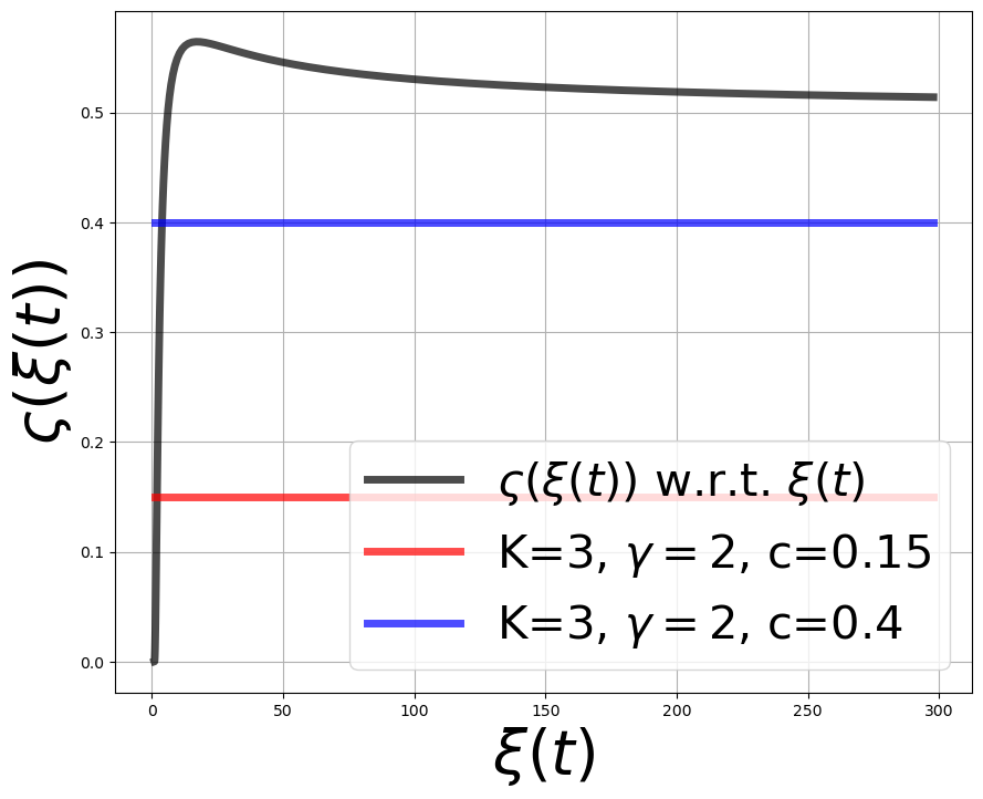
(a)

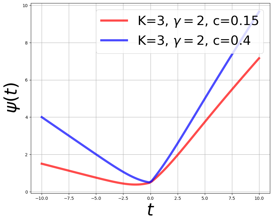
(b)

Figure 7: Illustration of the case of $\vartheta(\xi(0))\geq 0$, where $c=-K\sqrt{n\lambda_{\mathbf{W}}\lambda_{\mathbf{H}}}$.

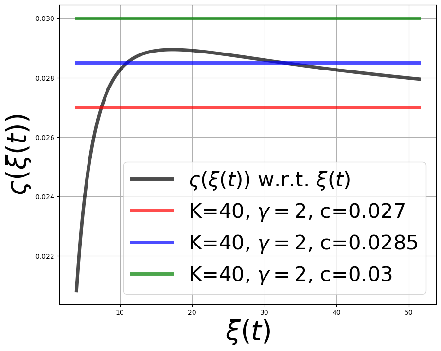
(a)

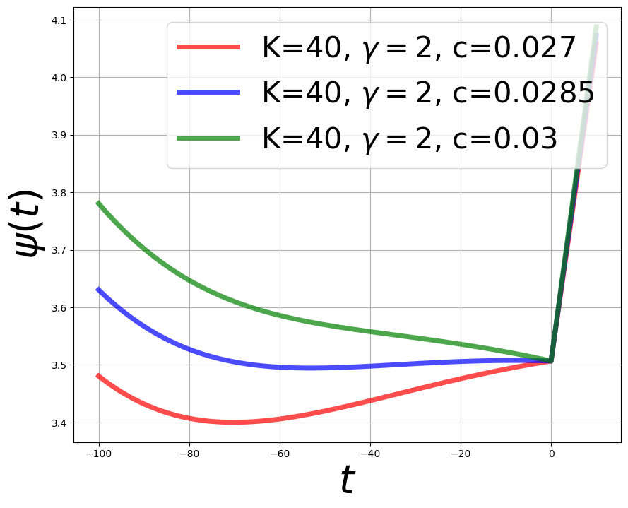
(b)

Figure 8: Illustration of the case of $\vartheta(\xi(0))<0$, where $c=K\sqrt{n\lambda_{\mathbf{W}}\lambda_{\mathbf{H}}}$.

3.3 LS is in GL

In this section, we will show that the LS defined in (LABEL:def:ls) belongs to the GL defined in Section 3. First, let us rewrite the LS definition in GL form as following:

$$\mathcal{L}_{\mathrm{LS}}(\bm{z},\bm{y}_{k})\; =\;-\left(1-\frac{(K-1)\alpha}{K}\right)\log\left(\frac{\exp(z_{k})}{\sum_{j=1}^{K}\exp(z_{j})}\right)-\frac{\alpha}{K}\sum_{\ell\neq k}^{K}\log\left(\frac{\exp(z_{\ell})}{\sum_{j=1}^{K}\exp(z_{j})}\right)$$

$$=\;\left(1-\frac{(K-1)\alpha}{K}\right)\log\left(\frac{\sum_{j=1}^{K}\exp(z_{j})}{\exp(z_{k})}\right)+\frac{\alpha}{K}\sum_{\ell\neq k}^{K}\log\left(\frac{\sum_{j=1}^{K}\exp(z_{j})}{\exp(z_{\ell})}\right)$$

$$=\;\left(1-\frac{(K-1)\alpha}{K}\right)\log\left(\sum_{j=1}^{K}\exp(z_{j}-z_{k}))\right)+\frac{\alpha}{K}\sum_{\ell\neq k}^{K}\log\left(\frac{\sum_{j=1}^{K}\exp(z_{j}-z_{k})}{\exp(z_{\ell}-z_{k})}\right)$$

$$=\;\log\left(\sum_{j=1}^{K}\exp(z_{j}-z_{k}))\right)-\frac{\alpha}{K}\sum_{\ell\neq k}^{K}(z_{\ell}-z_{k})$$

$$\geq\;\log\left(1+(K-1)\exp{\left(\frac{z_{j}-z_{k}}{K-1}\right)}\right)-\frac{\alpha}{K}\sum_{\ell\neq k}^{K}(z_{\ell}-z_{k})$$

where the inequality is due to the $\log$ is an increasing and function and $\exp$ is a strictly convex function, and it achieves equality only when $z_{j}=z_{j^{\prime}}$ for all $j,j^{\prime}\neq k$. Therefore, there exists such a function $\phi_{\text{LS}}$ to lower bound original LS loss $\mathcal{L}_{\mathrm{LS}}(\bm{z},\bm{y}_{k})$ as following:

$$\phi_{\text{LS}}(t)\; =\;\log\left(1+(K-1)\exp{\left(\frac{t}{K-1}\right)}\right)-\frac{\alpha}{K}t,$$

which satisfies the condition of (4). Next, we will show $\phi_{\text{LS}}(t)$ satisfies the condition (5). The first-order gradient of $\phi_{\text{LS}}(t)$ is following:

$$\nabla\phi_{\text{LS}}(t) =\frac{\exp{\left(\frac{t}{K-1}\right)}}{1+(K-1)\exp{\left(\frac{t}{K-1}\right)}}-\frac{\alpha}{K}$$

Let denote $\psi_{\text{LS}}(t)=\phi_{\text{LS}}(t)+c|t|$, then

• When $t\geq 0$: $\nabla\psi_{\text{LS}}(t)=\nabla\phi_{\text{LS}}(t)+c>0$ due to $\nabla\phi_{\text{LS}}(t)\geq 0\quad\text{for}\quad t>0$, thus the $\psi_{\text{LS}}(t)$ is an increasing function w.r.t. $t$, and the minimizer is achieved when $x=0$.

• When $t\leq 0$: $\nabla\psi_{\text{LS}}(t)=\nabla\phi_{\text{LS}}(t)-c$, and $\nabla\phi_{\text{LS}}(t)$ is an increasing function, which achieves minimizer when $t=0$ such that $\phi_{\text{LS}}(t)=\frac{1-\alpha}{K}$.

  • if $c\geq\frac{1-\alpha}{K}$, $\nabla\psi_{\text{LS}}(t)<0$, and $\psi(t)$ is a decreasing function for $t\leq 0$, and the minimizer is achieved when $t=0$;

  • if $0<c\leq\frac{1-\alpha}{K}$, there exist such $t^{*}$ such that $\nabla\psi_{\text{LS}}(t)=0$. When $t<t^{*}$, $\phi_{\text{LS}}(t)$ is a decreasing function; and when $t^{*}<t\leq 0$, $\phi_{\text{LS}}(t)$ is an increasing function. Therefore, the minimizer is achieved when $t=t^{*}<0$

Combing them together, we can prove that $\phi_{\text{LS}}$ satisfies the condition of (4).

4 Proof of LABEL:thm:global-minima for GL

In this part of appendices, we prove LABEL:thm:global-minima in LABEL:sec:main-results that we restate as follows.

[Global Optimality Condition of GL] Assume that the number of classes $K$ is smaller than feature dimension $d$, i.e., $K<d$, and the dataset is balanced for each class, $n=n_{1}=\cdots=n_{K}$. Then any global minimizer $(\bm{W}^{\star},\bm{H}^{\star},\bm{b}^{\star})$ of

$$\min_{\mathbf{W},\mathbf{H},\mathbf{b}}\;f(\mathbf{W},\mathbf{H},\mathbf{b})\; :=\;g(\bm{W}\bm{H}+\bm{b}\bm{1}^{\top})\;+\;\frac{\lambda_{\mathbf{W}}}{2}\left\|\mathbf{W}\right\|_{F}^{2}+\frac{\lambda_{\mathbf{H}}}{2}\left\|\mathbf{H}\right\|_{F}^{2}+\frac{\lambda_{\mathbf{b}}}{2}\left\|\mathbf{b}\right\|_{2}^{2},$$

with

$$g(\bm{W}\bm{H}+\bm{b}\bm{1}^{\top}):=\sum_{i=1}^{n}g(\bm{W}\bm{H}_{i}+\bm{b}\bm{1}^{\top}):=\frac{1}{N}\sum_{k=1}^{K}\sum_{i=1}^{n}\mathcal{L}(\bm{W}\bm{h}_{k,i}+\bm{b},\bm{y}_{k});$$ (7)

$$\mathcal{L}(\bm{W}\bm{h}_{k,i}+\bm{b},\bm{y}_{k})=\mathcal{L}(\bm{z}_{k,i},\bm{y}_{k})\text{ satisfying the the {Contrastive property} in \lx@cref{creftypecap~refnum}{def:GLoss-app}};$$ (8)

obeys the following

$$\left\|\mathbf{w}^{\star}\right\|_{2}\;=\;\left\|\mathbf{w}^{\star 1}\right\|_{2}\;=\;\left\|\mathbf{w}^{\star 2}\right\|_{2}\;=\;\cdots\;=\;\left\|\mathbf{w}^{\star K}\right\|_{2},\quad\text{and}\quad\mathbf{b}^{\star}=b^{\star}\mathbf{1},$$

$$\bm{h}_{k,i}^{\star}\;=\;\sqrt{\frac{\lambda_{\mathbf{W}}}{\lambda_{\mathbf{H}}n}}\bm{w}^{\star k},\quad\forall\;k\in[K],\;i\in[n],\quad\text{and}\quad\overline{\mathbf{h}}_{i}^{\star}\;:=\;\frac{1}{K}\sum_{j=1}^{K}\mathbf{h}_{j,i}^{\star}\;=\;\mathbf{0},\quad\forall\;i\in[n],$$

where either $b^{\star}=0$ or $\lambda_{\bm{b}}=0$, and the matrix $\bm{W}^{\star\top}$ is in the form of $K$-simplex ETF structure defined in Definition 1.2 in the sense that

$$\bm{W}^{\star\top}\bm{W}^{\star}\;=\;\left\|\mathbf{w}^{\star}\right\|_{2}^{2}\frac{K}{K-1}\left(\mathbf{I}_{K}-\frac{1}{K}\mathbf{1}_{K}\mathbf{1}_{K}^{\top}\right).$$

4.1 Main Proof

At a high level, we lower bound the general loss function based on the contrastive property (4), then check the equality conditions hold for the lower bounds and these equality conditions ensure that the global solutions $(\bm{W}^{\star},\bm{H}^{\star},\bm{b}^{\star})$ are in the form as shown in Section 4.

Proof [Proof of Section 4] First by Section 4.2, Section 4.2 and Section 4.2, we know that any critical point $(\mathbf{W},\mathbf{H},\mathbf{b})$ of $f$ in (4) satisfies

$$\bm{W}^{\top}\bm{W}=\frac{\lambda_{\bm{H}}}{\lambda_{\bm{W}}}\bm{H}\bm{H}^{\top};$$

$$\lambda_{\bm{H}}\bm{H}_{i}=-\bm{W}^{\top}\nabla_{\mathbf{Z}_{i}=\mathbf{W}\mathbf{H}_{i}}\;g(\bm{W}\bm{H}_{i}+\bm{b}\bm{1}^{\top});$$

$$\bm{b}=-\frac{\nabla g(\bm{W}\bm{H}+\bm{b}\bm{1}^{\top})}{\lambda_{\bm{b}}}\bm{1}.$$

For the rest of the proof, let $\bm{G}_{i}=\nabla_{\mathbf{Z}_{i}=\mathbf{W}\mathbf{H}_{i}}\;g(\bm{W}\bm{H}_{i}+\bm{b}\bm{1}^{\top})$ and $\tau=-\frac{\nabla g(\bm{W}\bm{H}+\bm{b}\bm{1}^{\top})}{\lambda_{\bm{b}}}$ to simplify the notations, and thus $\left\|\bm{H}\right\|_{F}^{2}=\frac{\lambda_{\bm{H}}}{\lambda_{\bm{W}}}\left\|\bm{W}\right\|_{F}^{2}$, $\lambda_{\bm{H}}\bm{H}_{i}=-\bm{W}^{\top}\bm{G}_{i}$ and $\bm{b}=\tau\bm{1}$.

We will first provide a lower bound for the general loss term $g(\bm{W}\bm{H}+\bm{b}\bm{1}^{\top})$ according to the Section 3, and then show that the lower bound is attained if and only if the parameters are in the form described in Section 4. By Lemma 4.2, we have

$$f(\mathbf{W},\mathbf{H},\mathbf{b})\; =\;g(\mathbf{W}\mathbf{H}+\mathbf{b}\mathbf{1}^{\top})\;+\;\frac{\lambda_{\mathbf{W}}}{2}\left\|\mathbf{W}\right\|_{F}^{2}+\frac{\lambda_{\mathbf{H}}}{2}\left\|\mathbf{H}\right\|_{F}^{2}+\frac{\lambda_{\mathbf{b}}}{2}\left\|\mathbf{b}\right\|_{2}^{2}$$

$$\geq\;\phi\left(\rho^{\star}\right)+K\sqrt{n\lambda_{\mathbf{W}}\lambda_{\mathbf{H}}}|\rho^{\star}|$$

where $\phi$ is lower bound function satisfying the Section 3, $\rho^{\star}=\arg\min_{\rho}\phi\left(\rho\right)+K\sqrt{n\lambda_{\mathbf{W}}\lambda_{\mathbf{H}}}|\rho|\leq 0$. Furthermore, by Section 4.2, we know that $\bar{\bm{Z}}_{i}^{\star}=\bm{W}^{\star}\bm{H}^{\star}_{i}=-\rho^{\star}\left(\mathbf{I}_{K}-\frac{1}{K}\mathbf{1}_{K}\mathbf{1}_{K}^{\top}\right)$, which satisfies the $K$-simplex ETF structure defined in Definition 1.2. In Section 4.2, we show the any minimizer $(\bm{W}^{\star},\bm{H}^{\star},\bm{b}^{\star})$ of $f(\mathbf{W},\mathbf{H},\mathbf{b})$ has following properties via check the equality conditions hold for the lower bounds in Section 4.2:

• $\left\|\bm{w}^{\star}\right\|_{2}\;=\;\left\|\bm{w}^{\star 1}\right\|_{2}\;=\;\left\|\bm{w}^{\star 2}\right\|_{2}\;=\;\cdots\;=\;\left\|\bm{w}^{\star K}\right\|_{2}$;

• $\mathbf{b}^{\star}=b^{\star}\mathbf{1}$, where either $b^{\star}=0$ or $\lambda_{\bm{b}}=0$;

• $\overline{\mathbf{h}}_{i}^{\star}\;:=\;\frac{1}{K}\sum_{j=1}^{K}\mathbf{h}_{j,i}^{\star}\;=\;\mathbf{0},\quad\forall\;i\in[n]$, and $\sqrt{\frac{\lambda_{\mathbf{W}}}{\lambda_{\mathbf{H}}n}}\bm{w}^{k\star}\;=\;\bm{h}_{k,i}^{\star},\quad\forall\;k\in[K],\;i\in[n]$;

• $\mathbf{W}\mathbf{W}^{\top}\;=\;\left\|\bm{w}^{\star}\right\|_{2}^{2}\frac{K-1}{K}\left(\mathbf{I}_{K}-\frac{1}{K}\mathbf{1}_{K}\mathbf{1}_{K}^{\top}\right)$;

The proof is complete.  

4.2 Supporting Lemmas

We first characterize the following balance property between $\bm{W}$ and $\bm{H}$ for any critical point $(\bm{W},\bm{H},\bm{b})$ of our loss function:

Let $\rho=\left\|\mathbf{W}\right\|_{F}^{2}$. Any critical point $(\bm{W},\bm{H},\bm{b})$ of (4) obeys

$$\bm{W}^{\top}\bm{W}\;=\;\frac{\lambda_{\bm{H}}}{\lambda_{\bm{W}}}\bm{H}\bm{H}^{\top}\quad\text{and}\quad\rho\;=\;\left\|\mathbf{W}\right\|_{F}^{2}\;=\;\frac{\lambda_{\bm{H}}}{\lambda_{\bm{W}}}\left\|\mathbf{H}\right\|_{F}^{2}.$$ (9)

Proof [Proof of Lemma 4.2] By definition, any critical point $(\bm{W},\bm{H},\bm{b})$ of (4) satisfies the following:

$$\nabla_{\bm{W}}f(\bm{W},\bm{H},\bm{b})\; =\;\nabla_{\mathbf{Z}=\mathbf{W}\mathbf{H}}\;g(\bm{W}\bm{H}+\bm{b}\bm{1}^{\top})\bm{H}^{\top}+\lambda_{\bm{W}}\bm{W}\;=\;\bm{0},$$ (10)

$$\nabla_{\bm{H}}f(\bm{W},\bm{H},\bm{b})\; =\;\bm{W}^{\top}\nabla_{\mathbf{Z}=\mathbf{W}\mathbf{H}}\;g(\bm{W}\bm{H}+\bm{b}\bm{1}^{\top})+\lambda_{\bm{H}}\bm{H}\;=\;\bm{0}.$$ (11)

Left multiply the first equation by $\mathbf{W}^{\top}$ on both sides and then right multiply second equation by $\bm{H}^{\top}$ on both sides, it gives

$$\mathbf{W}^{\top}\nabla_{\mathbf{Z}=\mathbf{W}\mathbf{H}}\;g(\bm{W}\bm{H}+\bm{b}\bm{1}^{\top})\bm{H}^{\top}\; =\;-\lambda_{\bm{W}}\mathbf{W}^{\top}\bm{W},$$

$$\mathbf{W}^{\top}\nabla_{\mathbf{Z}=\mathbf{W}\mathbf{H}}\;g(\bm{W}\bm{H}+\bm{b}\bm{1}^{\top})\bm{H}^{\top}\; =\;-\lambda_{\bm{H}}\mathbf{H}^{\top}\bm{H}.$$

Therefore, combining the equations above, we obtain

$$\lambda_{\bm{W}}\bm{W}^{\top}\bm{W}\;=\;\lambda_{\bm{H}}\bm{H}\bm{H}^{\top}.$$

Moreover, we have

$$\rho\;=\;\left\|\mathbf{W}\right\|_{F}^{2}\;=\;\operatorname{trace}\left(\mathbf{W}^{\top}\mathbf{W}\right)\;=\;\frac{\lambda_{\mathbf{H}}}{\lambda_{\mathbf{W}}}\operatorname{trace}\left(\mathbf{H}\mathbf{H}^{\top}\right)\;=\;\frac{\lambda_{\mathbf{H}}}{\lambda_{\mathbf{W}}}\operatorname{trace}\left(\mathbf{H}^{\top}\mathbf{H}\right)\;=\;\frac{\lambda_{\mathbf{H}}}{\lambda_{\mathbf{W}}}\left\|\mathbf{H}\right\|_{F}^{2},$$

as desired.  

Next, we characterize the following relationship per group between $\bm{W}$ and $\bm{H}_{i}$ for $i\in[n]$ for any critical $(\bm{W},\bm{H},\bm{b})$ of (4) satisfies the following:

Let $\bm{G}_{i}=\nabla_{\mathbf{Z}_{i}=\mathbf{W}\mathbf{H}_{i}}\;g(\bm{W}\bm{H}_{i}+\bm{b}\bm{1}^{\top})$. Any critical point $(\bm{W},\bm{H},\bm{b})$ of (4) obeys

$$\bm{W}^{\top}\bm{G}_{i}\;=\;-\lambda_{\bm{H}}\bm{H}_{i}.$$ (12)

Proof [Proof of Lemma 4.2] By definition, any critical point $(\bm{W},\bm{H},\bm{b})$ of (4) satisfies the following:

$$\nabla_{\bm{H}_{i}}f(\bm{W},\bm{H},\bm{b})\; =\;\bm{W}^{\top}\nabla_{\mathbf{Z}_{i}=\mathbf{W}\mathbf{H}_{i}}\;g(\bm{W}\bm{H}_{i}+\bm{b}\bm{1}^{\top})+\lambda_{\bm{H}}\bm{H}_{i}\;=\;\bm{0};$$ (13)

$$\bm{W}^{\top}\bm{G}_{i}\; =\;-\lambda_{\bm{H}}\bm{H}_{i}.$$ (14)

as desired.  

We then characterize the following isotropic property of $\bm{b}$ for any critical point $(\bm{W},\bm{H},\bm{b})$ of our loss function:

Let $\tau=-\frac{\nabla g(\bm{W}\bm{H}+\bm{b}\bm{1}^{\top})}{\lambda_{\bm{b}}}$. Any critical point $(\bm{W},\bm{H},\bm{b})$ of (4) obeys

$$\bm{b}\;=\;\tau\bm{1}.$$ (15)

Proof [Proof of Lemma 4.2] By definition, any critical point $(\bm{W},\bm{H},\bm{b})$ of (4) satisfies the following:

$$\nabla_{\bm{b}}f(\bm{W},\bm{H},\bm{b})\; =\;\nabla\;g(\bm{W}\bm{H}+\bm{b}\bm{1}^{\top})\bm{1}+\lambda_{\bm{b}}\bm{b}\;=\;\bm{0},$$

$$\bm{b}\; =\;-\frac{\nabla g(\bm{W}\bm{H}+\bm{b}\bm{1}^{\top})}{\lambda_{\bm{b}}}\bm{1}=\tau\bm{1}$$ (16)

as desired.  

Let $\mathbf{W}=\begin{bmatrix}(\mathbf{w}^{1})^{\top}\\ \vdots\\ (\mathbf{w}^{K})^{\top}\end{bmatrix}\in\mathbb{R}^{K\times d}$, $\mathbf{H}=\begin{bmatrix}\mathbf{H}_{1}&\mathbf{H}_{2}&\cdots&\mathbf{H}_{n}\end{bmatrix}\in\mathbb{R}^{d\times N}$, $\mathbf{H}_{i}=\begin{bmatrix}\mathbf{h}_{1,i}&\cdots&\mathbf{h}_{K,i}\end{bmatrix}\in\mathbb{R}^{d\times K}$, $\bar{\mathbf{Z}}=\bm{W}\bm{H}\in\mathbb{R}^{d\times N}$, $N=nK$, and $\bm{b}=\tau\bm{1}$. Given $g(\bm{W}\bm{H}+\bm{b}\bm{1}^{\top}_{K})$ defined in (7), for any critical point $(\bm{W},\bm{H},\bm{b})$ of (4), it satisfies

$$f(\mathbf{W},\mathbf{H},\mathbf{b}) \geq\phi\left(\rho^{\star}\right)+(K-1)\sqrt{n\lambda_{\mathbf{W}}\lambda_{\mathbf{H}}}|\rho^{\star}|$$ (17)

$$\bar{\bm{Z}}^{\star} =-\rho^{\star}\left(\mathbf{I}_{K}-\frac{1}{K}\mathbf{1}_{K}\mathbf{1}_{K}^{\top}\right){\mathbf{I}_{K}^{n}}$$ (18)

where $\phi$ is lower bound function satisfying the Section 3, $\rho^{\star}=\arg\min_{\rho}\phi\left(\rho\right)+K\sqrt{n\lambda_{\mathbf{W}}\lambda_{\mathbf{H}}}|\rho|$, and $\bar{\mathbf{Z}}^{\star}=\bm{W}^{\star}\bm{H}^{\star}$.

Proof [Proof of Lemma 4.2] With $\bar{\mathbf{Z}}_{i}=\bm{W}\bm{H}_{i}$, and $\left\|\bar{\mathbf{Z}}_{i}\right\|_{2}=\sigma_{i}^{\max}$, we have the following lower bound for $f(\mathbf{W},\mathbf{H},\mathbf{b})$ as

$$\begin{split}f(\mathbf{W},\mathbf{H},\mathbf{b})&=g(\bm{W}\bm{H}+\bm{b}\bm{1}^{\top})+\frac{\lambda_{\mathbf{W}}}{2}\left\|\mathbf{W}\right\|_{F}^{2}+\frac{\lambda_{\mathbf{H}}}{2}\left\|\mathbf{H}\right\|_{F}^{2}+\frac{\lambda_{\mathbf{b}}}{2}\left\|\mathbf{b}\right\|_{2}^{2}\\ \;&=\;\sum_{i=1}^{n}\left(g(\bm{W}\bm{H}_{i}+\bm{b}\bm{1}^{\top})+\frac{\lambda_{\mathbf{W}}}{2n}\left\|\mathbf{W}\right\|_{F}^{2}+\frac{\lambda_{\mathbf{H}}}{2}\left\|\mathbf{H}_{i}\right\|_{F}^{2}\right)+\frac{\lambda_{\mathbf{b}}}{2}\left\|\mathbf{b}\right\|_{2}^{2}\\ \;&\geq\;\sum_{i=1}^{n}\left(g(\bar{\mathbf{Z}}_{i}+\bm{b}\bm{1}^{\top})+\sqrt{\lambda_{\mathbf{W}}\lambda_{\mathbf{H}}/n}\left\|\bar{\mathbf{Z}}_{i}\right\|_{*}\right)+\frac{\lambda_{\mathbf{b}}}{2}\left\|\mathbf{b}\right\|_{2}^{2}\\ \;&\geq\;\sum_{i=1}^{n}\left(g(\bar{\mathbf{Z}}_{i}+\bm{b}\bm{1}^{\top})+\sqrt{\lambda_{\mathbf{W}}\lambda_{\mathbf{H}}/n}\frac{\left\|\bar{\mathbf{Z}}\right\|_{F}^{2}}{\left\|\bar{\mathbf{Z}}_{i}\right\|_{2}}\right)+\frac{\lambda_{\mathbf{b}}}{2}\left\|\mathbf{b}\right\|_{2}^{2}\\ \;&=\;\sum_{i=1}^{n}\left(g(\bar{\mathbf{Z}}_{i}+\bm{b}\bm{1}^{\top})+\frac{\sqrt{\lambda_{\mathbf{W}}\lambda_{\mathbf{H}}/n}}{\sigma_{i}^{\max}}\left\|\bar{\mathbf{Z}}_{i}\right\|_{F}^{2}\right)+\frac{\lambda_{\mathbf{b}}}{2}\left\|\mathbf{b}\right\|_{2}^{2},\end{split}$$

where the first inequality is from Section 1.2, and the second inequality becomes equality only when $\bar{\bm{Z}}_{i}\neq\bm{0}$ and

$$\begin{split}\forall\;k,\sigma_{k}(\bar{\bm{Z}}_{i})&=\sigma_{i}^{\max}\text{ or }0\\ \exists\;k,\sigma_{k}(\bar{\bm{Z}}_{i})&\neq 0\end{split}$$ (19)

where $\sigma_{k}(\bar{\bm{Z}}_{i})$ is the $k$-th singular value of $\bar{\bm{Z}}_{i}$. While we only consider $\bar{\bm{Z}}_{i}\neq\bm{0}$, we will show the $\bar{\bm{Z}}_{i}=\bm{0}$ can be included in an uniform form as following proof. We can further bound $f(\mathbf{W},\mathbf{H},\mathbf{b})$ by

$$f(\mathbf{W},\mathbf{H},\mathbf{b})\;\geq\;\sum_{i=1}^{n}\left(g(\bar{\mathbf{Z}}_{i}+\bm{b}\bm{1}^{\top})+\frac{\sqrt{\lambda_{\mathbf{W}}\lambda_{\mathbf{H}}/n}}{\sigma_{i}^{\max}}\left\|\bar{\mathbf{Z}}_{i}\right\|_{F}^{2}\right)+\frac{\lambda_{\mathbf{b}}}{2}\left\|\mathbf{b}\right\|_{2}^{2},$$

$$\;\geq\; \frac{1}{N}\sum_{k=1}^{K}\sum_{i=1}^{n}\phi\left(\sum_{j\neq k}\left(\bar{z}_{k,i,j}-\bar{z}_{k,i,k}+\underbrace{b_{j}-b_{k}}_{=0}\right)\right)+\sum_{i=1}^{n}\frac{\sqrt{\lambda_{\mathbf{W}}\lambda_{\mathbf{H}}/n}}{\sigma_{i}^{\max}}\left\|\bar{\mathbf{Z}}_{i}\right\|_{F}^{2}+\frac{\lambda_{\mathbf{b}}}{2}\left\|\mathbf{b}\right\|_{2}^{2},$$

$$\;=\; \frac{1}{N}\sum_{i=1}^{n}\sum_{k=1}^{K}\left(\phi\left(\sum_{j\neq k}^{K}\left(\bar{z}_{k,i,j}-\bar{z}_{k,i,k}\right)\right)+\frac{K\sqrt{n\lambda_{\mathbf{W}}\lambda_{\mathbf{H}}}}{\sigma_{i}^{\max}}\left\|\mathbf{\bar{}}{z}_{k,i}\right\|_{2}^{2}\right)+\frac{\lambda_{\mathbf{b}}}{2}\left\|\mathbf{b}\right\|_{2}^{2},$$ (20)

where the first inequality is from the first condition (4) of loss function $\mathcal{L}$ and the equality achieves only when $\bar{z}_{k,i,j}=\bar{z}_{k,i,j^{\prime}}$ for $j\neq k,j^{\prime}\neq k$, and $b_{j}-b_{k}=0$ is due to Section 4.2. If we denote by $\rho_{k,i}=\sum_{j\neq k}^{K}\left(\bar{z}_{k,i,j}-\bar{z}_{k,i,k}\right)/(K-1)$, then

$$\left\|\bar{\bm{z}}_{k,i}\right\|_{2}^{2} =\sum_{j\neq k}\bar{z}^{2}_{k,i,j}+\bar{z}^{2}_{k,i,k}$$

$$\geq(K-1)\left(\sum_{j\neq k}\frac{\bar{z}_{k,i,j}}{K-1}\right)^{2}+\bar{z}_{k,i,k}$$

$$=(K-1)\left(\sum_{j\neq k}\frac{\bar{z}_{k,i,j}-\bar{z}_{k,i,k}}{K-1}+\bar{z}_{k,i,k}\right)^{2}+\bar{z}_{k,i,k}$$

$$=(K-1)\left(\rho_{k,i}+\bar{z}_{k,i,k}\right)^{2}+\bar{z}_{k,i,k}$$

$$\geq\frac{K-1}{K}\rho_{k,i}^{2}$$

where the first inequality achieves equality only when $\bar{z}_{k,i,j}=\bar{z}_{k,i,j^{\prime}}$ for $j\neq k,j^{\prime}\neq k$, and the last line achieves equality only when $\bar{z}_{k,i,k}=-\frac{K-1}{K}\rho_{k,i}$, thus $\bar{z}_{k,i,j}=\frac{1}{K}\rho_{k,i}$ for $j\neq k$. Denoting $\mathbf{\rho}_{i}=\begin{bmatrix}\rho_{i,1}&\rho_{i,2}&\cdots&\rho_{i,K}\end{bmatrix}$ and $\text{diag}(\mathbf{\rho}_{i})$ is a diagonal matrix using $\mathbf{\rho}_{i}$ as diagonal entries, and supposing $|\rho_{1}|\geq|\rho_{2}|>\cdots>|\rho_{K}|$, we can express $\bar{\bm{Z}}_{i}$ as:

$$\bar{\bm{Z}}_{i} =-(\mathbf{I}_{K}-\frac{1}{K}\bm{1}_{K}\bm{1}^{\top}_{K})\text{diag}(\mathbf{\rho}_{i}),$$ (21)

and we can extend the expression of (20) as following

$$f(\mathbf{W},\mathbf{H},\mathbf{b})\;\geq\; \frac{1}{N}\sum_{i=1}^{n}\sum_{k=1}^{K}\left(\underbrace{\phi\left(\rho_{k,i}\right)+\frac{(K-1)\sqrt{n\lambda_{\mathbf{W}}\lambda_{\mathbf{H}}}}{\sigma_{i}^{\max}}\rho_{k,i}^{2}}_{\psi(\rho_{k,i})}\right)+\frac{\lambda_{\bm{b}}}{2}\left\|\bm{b}\right\|_{2}$$ (22)

which is decouplable if we treat the $i$-th samples per class as a group, thus we only consider the $i$-th samples per class. In the next part, denote $\rho^{\star}=\arg\min_{\rho}\phi\left(\rho\right)+(K-1)\sqrt{n\lambda_{\mathbf{W}}\lambda_{\mathbf{H}}}|\rho|$.

When $K\geq 3$, according to the $\bm{Z}=-(\mathbf{I}_{K}-\frac{1}{K}\bm{1}_{K}\bm{1}^{\top}_{K})\text{diag}(\mathbf{\rho}_{i})$, the condition of (19) and Section 1.2, we know $\bm{Z}$ has only two possible forms corresponding to two different objective value of $\sum_{k=1}^{K}\psi(\rho_{k})$ such that

• $|\rho_{1}|=|\rho_{2}|=\cdots=|\rho_{K}|$: we can have $\sigma_{\max}=|\rho_{1}|$ and

  $$\sum_{k=1}^{K}\psi(\rho_{k}) =\sum_{k=1}^{K}\left(\phi\left(\rho_{k}\right)+\frac{(K-1)\sqrt{n\lambda_{\mathbf{W}}\lambda_{\mathbf{H}}}}{\sigma^{\max}}\rho_{k}^{2}\right)$$

  $$=\sum_{k=1}^{K}\left(\phi\left(\rho_{k}\right)+(K-1)\sqrt{n\lambda_{\mathbf{W}}\lambda_{\mathbf{H}}}|\rho_{k}|\right)$$

  $$\geq K\left(\phi\left(\rho^{\star}\right)+(K-1)\sqrt{n\lambda_{\mathbf{W}}\lambda_{\mathbf{H}}}|\rho^{\star}|\right)$$

  where the last line holds equality only when $|\rho_{1}|=|\rho_{2}|=\cdots=|\rho_{K}|=\rho^{*}$.

• $|\rho_{2}|=\cdots=|\rho_{K}|=0$: we can have $\sigma_{\max}=\sqrt{(K-1)/K}|\rho_{1}|$ and

  $$\sum_{k=1}^{K}\psi(\rho_{k}) =\phi\left(\rho_{1}\right)+(K-1)\sqrt{n\lambda_{\mathbf{W}}\lambda_{\mathbf{H}}}\sqrt{\frac{K}{K-1}}|\rho_{1}|+(K-1)\phi\left(0\right)$$

  $$=\phi\left(\rho_{1}\right)+(K-1)\sqrt{n\lambda_{\mathbf{W}}\lambda_{\mathbf{H}}}|\rho_{1}|$$

  $$\;+(K-1)\sqrt{n\lambda_{\mathbf{W}}\lambda_{\mathbf{H}}}\left(\sqrt{\frac{K}{K-1}}-1\right)|\rho_{1}|+(K-1)\phi\left(0\right)$$

  $$\geq K\left(\phi\left(\rho^{\star}\right)+(K-1)\sqrt{n\lambda_{\mathbf{W}}\lambda_{\mathbf{H}}}|\rho^{\star}|\right)$$

  where the last line holds equality only when $|\rho_{1}|=\cdots=|\rho_{K}|=|\rho^{\star}|=0$.

When $K=2$, according to the Section 1.2, we can calculate $\sigma_{\max}=\sqrt{\frac{\rho_{1}^{2}+\rho_{2}^{2}}{2}}$, then

$$\sum_{k=1}^{2}\psi(\rho_{i}) =\phi\left(\rho_{1}\right)+\phi\left(\rho_{2}\right)+\frac{(K-1)\sqrt{n\lambda_{\mathbf{W}}\lambda_{\mathbf{H}}}}{\sigma^{\max}}\left(\rho_{1}^{2}+\rho_{2}^{2}\right)$$

$$=\phi\left(\rho_{1}\right)+\phi\left(\rho_{2}\right)+(K-1)\sqrt{n\lambda_{\mathbf{W}}\lambda_{\mathbf{H}}}\sqrt{2(\rho_{1}^{2}+\rho_{2}^{2})}$$

$$=\phi\left(\rho_{1}\right)+(K-1)\sqrt{n\lambda_{\mathbf{W}}\lambda_{\mathbf{H}}}|\rho_{1}|+\phi\left(\rho_{2}\right)+(K-1)\sqrt{n\lambda_{\mathbf{W}}\lambda_{\mathbf{H}}}|\rho_{2}|$$

$$\;+(K-1)\sqrt{n\lambda_{\mathbf{W}}\lambda_{\mathbf{H}}}\left(\sqrt{2(\rho_{1}^{2}+\rho_{2}^{2})}-|\rho_{1}|-|\rho_{2}|\right)$$

$$\geq 2\left(\phi\left(\rho^{\star}\right)+(K-1)\sqrt{n\lambda_{\mathbf{W}}\lambda_{\mathbf{H}}}|\rho^{\star}|\right)$$

where the last line holds equality only when $|\rho_{1}|=|\rho_{2}|=|\rho^{\star}|$.

Combining them together, for $K\geq 2$, we can further extend the expression of (22) as following

$$f(\mathbf{W},\mathbf{H},\mathbf{b})\;\geq\; \frac{1}{N}\sum_{i=1}^{n}\sum_{k=1}^{K}\left(\phi\left(\rho_{k,i}\right)+\frac{(K-1)\sqrt{n\lambda_{\mathbf{W}}\lambda_{\mathbf{H}}}}{\sigma_{i}^{\max}}\rho_{k,i}^{2}\right)+\frac{\lambda_{\bm{b}}}{2}\left\|\bm{b}\right\|_{2}$$

$$\;\geq\; \frac{1}{N}\sum_{i=1}^{n}K\left(\phi\left(\rho^{\star}\right)+(K-1)\sqrt{n\lambda_{\mathbf{W}}\lambda_{\mathbf{H}}}|\rho^{\star}|\right)+\frac{\lambda_{\bm{b}}}{2}\left\|\bm{b}\right\|_{2}$$

$$\;\geq\; \phi\left(\rho^{\star}\right)+(K-1)\sqrt{n\lambda_{\mathbf{W}}\lambda_{\mathbf{H}}}|\rho^{\star}|$$ (23)

where the last equation is achieved when $\bm{b}=\mathbf{0}$ or $\lambda_{\bm{b}}=0$. According to the condition (5) of loss function $\mathcal{L}$ that the minimizer $\rho^{\star}$ of $\phi(\rho)+c|\rho|$ is unique for any $c>0$, and by denoting $\mathbf{I}_{K}^{n}=\begin{bmatrix}\mathbf{I}_{K}&\cdots&\mathbf{I}_{K}\end{bmatrix}\in\mathbb{R}^{K\times nK}$, we have

$$\bar{\bm{Z}}_{i}^{\star} =-\rho^{\star}\left(\mathbf{I}_{K}-\frac{1}{K}\mathbf{1}_{K}\mathbf{1}_{K}^{\top}\right)$$ (24)

$$\bar{\bm{Z}}^{\star} =-\rho^{\star}\left(\mathbf{I}_{K}-\frac{1}{K}\mathbf{1}_{K}\mathbf{1}_{K}^{\top}\right){\mathbf{I}_{K}^{n}}$$ (25)

as desired.  

Next, we show that the lower bound in (17) is attained if and only if $(\mathbf{W},\mathbf{H},\mathbf{b})$ satisfies the following conditions. Under the same assumptions of Lemma 4.2, the lower bound in (17) is attained for any minimizer $(\mathbf{W}^{\star},\mathbf{H}^{\star},\mathbf{b}^{\star})$ of (4) if and only if the following hold

$$\left\|\mathbf{w}^{\star}\right\|_{2}\;=\;\left\|\mathbf{w}^{\star 1}\right\|_{2}\;=\;\left\|\mathbf{w}^{\star 2}\right\|_{2}\;=\;\cdots\;=\;\left\|\mathbf{w}^{\star K}\right\|_{2},\quad\text{and}\quad\mathbf{b}^{\star}=b^{\star}\mathbf{1},$$

$$\bm{h}_{k,i}^{\star}\;=\;\sqrt{\frac{\lambda_{\mathbf{W}}}{\lambda_{\mathbf{H}}n}}\bm{w}^{\star k},\quad\forall\;k\in[K],\;i\in[n],\quad\text{and}\quad\overline{\mathbf{h}}_{i}^{\star}\;:=\;\frac{1}{K}\sum_{j=1}^{K}\mathbf{h}_{j,i}^{\star}\;=\;\mathbf{0},\quad\forall\;i\in[n],$$

where either $b^{\star}=0$ or $\lambda_{\bm{b}}=0$, and the matrix $\bm{W}^{\star\top}$ is in the form of $K$-simplex ETF structure (see appendix for the formal definition) in the sense that

$$\bm{W}^{\star\top}\bm{W}^{\star}\;=\;\left\|\mathbf{w}^{\star}\right\|_{2}^{2}\frac{K}{K-1}\left(\mathbf{I}_{K}-\frac{1}{K}\mathbf{1}_{K}\mathbf{1}_{K}^{\top}\right).$$

The proof of Section 4.2 utilizes the Lemma Section 4.2, Section 4.2 and Section 4.2, and the conditions (23) and the structure of $\bar{\mathbf{Z}}^{\star}$ (25) during the proof of Lemma 4.2.

Proof [Proof of Lemma 4.2] From the (25), we know that $\bar{\mathbf{Z}}^{\star}_{1}=\bar{\mathbf{Z}}^{\star}_{2}=\cdots=\bar{\mathbf{Z}}^{\star}_{n}$ and then $\bm{G}_{i}^{\star}=\nabla_{\bar{\mathbf{Z}}^{\star}_{i}=\bm{W}^{\star}\bm{H}^{\star}_{i}}g(\bm{W}^{\star}\bm{H}^{\star}_{i}+\bm{b}\bm{1}^{\top})$ is equivalent for $i\in[n]$. Let denote $\bm{G}^{\star}=\bm{G}^{\star}_{1}=\bm{G}^{\star}_{2}=\cdots=\bm{G}^{\star}_{n}$, the (12) in Lemma 4.2 can be expressed as:

$${\bm{W}^{\star}}^{\top}\bm{G}^{\star} =-\lambda_{\bm{H}}\bm{H}_{i}^{\star}$$

Therefore, $\tilde{\bm{H}}^{\star}=\bm{H}_{1}^{\star}=\bm{H}_{2}^{\star}=\cdots=\bm{H}_{n}^{\star}$, which means the last-layer features from different classes are collapsed to their corresponding class-mean $\bm{h}_{k,1}^{\star}=\bm{h}_{k,2}^{\star}=\cdots=\bm{h}_{k,n}^{\star}$, for $k\in[K]$. Furthermore, $\bm{H}^{\star}\bm{H}^{\star\top}=n\tilde{\bm{H}}^{\star}\tilde{\bm{H}}^{\star\top}$, combining this with (9) in Lemma 4.2, we know that

$$\lambda_{\bm{W}}\bm{W}^{\star\top}\bm{W}^{\star}\;=\;\lambda_{\bm{H}}\bm{H}^{\star}\bm{H}^{\star\top}=n\lambda_{\bm{H}}\tilde{\bm{H}}^{\star}\tilde{\bm{H}}^{\star\top}$$

By denoting $\bm{W}^{\star}={\bm{U}_{\bm{W}}}{\bm{\Sigma}_{\bm{W}}}{\bm{V}^{\top}_{\bm{W}}}$ and ${\tilde{\bm{H}}^{\star}}={\bm{U}_{\tilde{\bm{H}}}}{\bm{\Sigma}_{\tilde{\bm{H}}}}{\bm{V}^{\top}_{\tilde{\bm{H}}}}$, where $\bm{U}_{\bm{W}}$, $\bm{\Sigma}_{\bm{W}}$, $\bm{V}^{\top}_{\bm{W}}$ are the left singular vector matrix, singular value matrix, and right singular vector matrix of $\bm{W}^{\star}$, respectively; and $\bm{U}_{\tilde{\bm{H}}^{\star}}$, $\bm{\Sigma}_{\tilde{\bm{H}}^{\star}}$, $\bm{V}_{{\tilde{\bm{H}}}^{\star}}^{\top}$ are the left singular vector matrix, singular value matrix, and right singular vector matrix of $\tilde{\bm{H}}$, respectively, we can get

$$\bm{V}^{\top}_{\bm{W}} =\bm{U}_{\tilde{\bm{H}}}$$

$$\bm{\Sigma}_{\bm{W}} =\sqrt{\frac{n\lambda_{\bm{H}}}{\lambda_{\bm{W}}}}\bm{\Sigma}_{\tilde{\bm{H}}}$$

Therefore, $\bm{Z}_{i}^{\star}=\bm{W}^{\star}\tilde{\bm{H}}^{\star}=\sqrt{\frac{\lambda_{\bm{W}}}{n\lambda_{\bm{H}}}}\bm{U}_{\bm{W}}\mathbf{\Sigma}^{2}_{\bm{W}}\bm{V}^{\top}_{\tilde{\bm{H}}}$. According to the $\bm{Z}_{i}=-\rho^{\star}(\mathbf{I}_{K}-\frac{1}{K}\bm{1}_{K}\bm{1}_{K}^{\top})$ in (24) and $\rho^{\star}\leq 0$, which is symmetric, thus, $\bm{U}_{\bm{W}}=\bm{V}_{\tilde{\bm{H}}}$, $\bm{W}^{\star}=\sqrt{\frac{n\lambda_{\bm{H}}}{\lambda_{\bm{W}}}}\tilde{\bm{H}}^{\star\top}$, that is, $\bm{w}^{\star k}\;=\;\sqrt{\frac{n\lambda_{\bm{H}}}{\lambda_{\bm{W}}}}\bm{h}^{\star}_{k,i},\quad\forall\;k\in[K],\;i\in[n]$ and

$$\bm{Z}_{i}^{\star} =\sqrt{\frac{\lambda_{\bm{W}}}{n\lambda_{\bm{H}}}}\bm{W}^{\star}\bm{W}^{\star\top}=\sqrt{\frac{\lambda_{\bm{W}}}{n\lambda_{\bm{H}}}}\bm{W}^{\star}\bm{W}^{\star}$$

$$=-\rho^{\star}(\mathbf{I}_{K}-\frac{1}{K}\bm{1}_{K}\bm{1}_{K}^{\top})=-\rho^{\star}(\mathbf{I}_{K}-\frac{1}{K}\bm{1}_{K}\bm{1}_{K}^{\top})(\mathbf{I}_{K}-\frac{1}{K}\bm{1}_{K}\bm{1}_{K}^{\top})$$

$$\bm{W}^{\star} =(\frac{\rho^{\star 2}n\lambda_{\bm{H}}}{\lambda_{\bm{W}}})^{\frac{1}{4}}(\mathbf{I}_{K}-\frac{1}{K}\bm{1}_{K}\bm{1}_{K}^{\top})$$

$$\tilde{\bm{H}}^{\star} =(\frac{\rho^{\star 2}\lambda_{\bm{W}}}{\lambda_{\bm{H}}})^{\frac{1}{4}}(\mathbf{I}_{K}-\frac{1}{K}\bm{1}_{K}\bm{1}_{K}^{\top})$$

Therefore,

$$\left\|\mathbf{w}^{\star 1}\right\|_{2}\;=\;\left\|\mathbf{w}^{\star 2}\right\|_{2}\;=\;\cdots\;=\;\left\|\mathbf{w}^{\star K}\right\|_{2}$$

$$\overline{\mathbf{h}}_{i}^{\star}\;:=\;\frac{1}{K}\sum_{j=1}^{K}\mathbf{h}_{j,i}^{\star}\;=\;\mathbf{0},\quad\forall\;i\in[n]$$

where $\overline{\mathbf{h}}_{i}^{\star}=\sum_{k=1}^{K}(\bm{h}_{k,i}^{\star})$ and according to the condition of (23) and Lemma 4.2, $\bm{b}^{\star}=\mathbf{0}$ or $\lambda_{\bm{b}}=0$.  

5 Proof of LABEL:cor:global-geometry-LS and LABEL:cor:global-geometry-FL

Following LABEL:thm:global-geometry, we only need to prove convexity for label smoothing and local convexity for focal loss.

For any output (logit) $\bm{z}\in\mathbb{R}^{K}$, define

$$\bm{p}=\sigma(\bm{z})\in\mathbb{R}^{K},\ \text{where}\ p_{i}=\frac{\exp(z_{i})}{\sum_{j=1}^{K}\exp(z_{j})}.$$

Let $\bm{y}^{\text{smooth}}\in\mathbb{R}^{K}$ be the label vector with $0\leq y^{\text{smooth}}_{i}\leq 1$ and $\sum_{i}y^{\text{smooth}}_{i}=1$. The three loss functions can be written as

$$f(\bm{z})=\sum_{i=1}^{K}y^{\text{smooth}}_{i}\xi(p_{i}).$$

Some useful properties:

$$\partial_{z_{i}}\xi(p_{k})=\begin{cases}\xi^{\prime}(p_{k})(p_{k}-p_{k}^{2}),&i=k,\\ -\xi^{\prime}(p_{k})p_{k}p_{i},&i\neq k,\end{cases}\ \Longrightarrow\ \nabla_{\bm{z}}\xi(p_{k})=\xi^{\prime}(p_{k})p_{k}(\bm{e}_{k}-\bm{p})$$

$$\partial_{z_{i}}p_{k}=\begin{cases}p_{k}-p_{k}^{2},&i=k,\\ -p_{k}p_{i},&i\neq k,\end{cases}\ \Longrightarrow\ \nabla_{\bm{z}}\bm{p}=\nabla_{\bm{z}}\sigma(\bm{z})=\operatorname{diag}(\bm{p})-\bm{p}\bm{p}^{\top}$$

Therefore, the gradient and Hessian of $f(\bm{z})$ are given by

$$\nabla f(\bm{z}) =\sum_{i=1}^{K}y^{\text{smooth}}_{i}\nabla_{\bm{z}}\xi(p_{i})=\sum_{i=1}^{K}y^{\text{smooth}}_{i}\underbrace{\xi^{\prime}(p_{i})p_{i}}_{\eta(p_{i})}(\bm{1}_{i}-\bm{p})$$ (26)

$$\nabla^{2}f(\bm{z}) =\nabla(\nabla f(\bm{z}))=\sum_{i=1}^{K}y^{\text{smooth}}_{i}\left(\eta^{\prime}(p_{i})p_{i}\underbrace{(\bm{1}_{i}-\bm{p})(\bm{1}_{i}-\bm{p})^{\top}}_{\bm{0}}-\eta(p_{i})\underbrace{\left(\operatorname{diag}(\bm{p})-\bm{p}\bm{p}^{\top}\right)}_{\succeq\bm{0}}\right)$$

Thus, $\nabla^{2}f(\bm{z})$ is PSD when $\eta(p_{i})\leq 0$ and $\eta^{\prime}(p_{i})\geq 0$ for all $i$, i.e.,

$$\xi^{\prime}(p_{i})\leq 0,\quad\xi^{\prime\prime}(p_{i})p_{i}+\xi^{\prime}(p_{i})\geq 0.$$ (27)

Now we consider the following cases:

• CE loss with $\bm{y}^{\text{smooth}}=\bm{e}_{k}$ and $\xi(t)=-\log(t)$. In this case, $\xi^{\prime}(p_{i})=-\frac{1}{p_{i}}$ and $\eta(p_{i})=\xi^{\prime}(p_{i})p_{i}=-1$, and thus

  $$\nabla^{2}f(\bm{z})=\operatorname{diag}(\bm{p})-\bm{p}\bm{p}^{\top}\succeq\bm{0},$$

  where the inequality can be obtained by the Gershgorin circle theorem.

• Label smoothing with $\bm{y}^{\text{smooth}}=(1-\alpha)\bm{e}_{k}+\frac{\alpha}{K}\bm{1}$ and $\xi(t)=-\log(t)$. In this case, $\xi^{\prime}(p_{i})=-\frac{1}{p_{i}}$ and $\eta(p_{i})=\xi^{\prime}(p_{i})p_{i}=-1$, and thus

  $$\nabla^{2}f(\bm{z})=\sum_{i=1}^{K}y^{\text{smooth}}_{i}\left(\operatorname{diag}(\bm{p})-\bm{p}\bm{p}^{\top}\right)=\operatorname{diag}(\bm{p})-\bm{p}\bm{p}^{\top}\succeq\bm{0}$$

  since $\sum_{i=1}^{K}y^{\text{smooth}}_{i}=1$.

• Focal loss with $\bm{y}^{\text{smooth}}=\bm{e}_{k}$ and $\xi(t)=-(1-t)^{\beta}\log(t)$. In this case,

  $$\xi^{\prime}(p_{i}) =\beta(1-p_{i})^{\beta-1}\log(p_{i})-\frac{(1-p_{i})^{\beta}}{p_{i}},$$

  $$\eta(p_{i}) =\xi^{\prime}(p_{i})p_{i}=\beta p_{i}(1-p_{i})^{\beta-1}\log(p_{i})-(1-p_{i})^{\beta}\leq 0,\ \forall\ \beta\geq 0,p_{i}\in[0,1],$$

  $$\eta^{\prime}(p_{i}) =\beta(1-p_{i})^{\beta-1}\log(p_{i})-\beta(\beta-1)p_{i}(1-p_{i})^{\beta-2}\log(p_{i})+\beta(1-p_{i})^{\beta-1}+\beta(1-p_{i})^{\beta-1}$$

  $$=\beta(1-p_{i})^{\beta-2}\left((1-\beta p_{i})\log(p_{i})+2(1-p_{i})\right)$$

  $$\geq\beta(1-p_{i})^{\beta-2}\left(\log(p_{i})+2(1-p_{i})\right).$$

  Thus, $\eta^{\prime}(p_{i})\geq 0$ whenever $0.21\leq p_{i}\leq 1$. The Hessian becomes

  $$\nabla^{2}f(\bm{z}) =\eta^{\prime}(p_{k})p_{k}\underbrace{(\bm{e}_{k}-\bm{p})(\bm{e}_{k}-\bm{p})^{\top}}_{\succeq\bm{0}}-\eta(p_{k})\underbrace{\left(\operatorname{diag}(\bm{p})-\bm{p}\bm{p}^{\top}\right)}_{\succeq\bm{0}}$$

  which is PSD when $0.21\leq p_{k}\leq 1$.