DISCOVER: Deep identification of symbolically concise open-form PDEs via enhanced reinforcement-learning

Abstract

The working mechanisms of complex natural systems tend to abide by concise and profound partial differential equations (PDEs). Methods that directly mine equations from data are called PDE discovery, which reveals consistent physical laws and facilitates our adaptive interaction with the natural world. In this paper, an enhanced deep reinforcement-learning framework is proposed to uncover symbolically concise open-form PDEs with little prior knowledge. Particularly, based on a symbol library of basic operators and operands, a structure-aware recurrent neural network agent is designed and seamlessly combined with the sparse regression method to generate concise and open-form PDE expressions. All of the generated PDEs are evaluated by a meticulously designed reward function by balancing fitness to data and parsimony, and updated by the model-based reinforcement learning in an efficient way. Customized constraints and regulations are formulated to guarantee the rationality of PDEs in terms of physics and mathematics. The experiments demonstrate that our framework is capable of mining open-form governing equations of several dynamic systems, even with compound equation terms, fractional structure, and high-order derivatives, with excellent efficiency. Without the need for prior knowledge, this method shows great potential for knowledge discovery in more complicated circumstances with exceptional efficiency and scalability.
Keywords: PDE discovery; symbolic representation; deep reinforcement learning; structure-aware LSTM agent.

The laws of physics reveal how the world around us works. Many phenomena in dynamic natural systems can be described by concise and elegant governing equations. The exploration of these equations can be done in two ways: (1) induction, which involves deriving equations directly from data (e.g., Kepler’s laws were built upon Brahe’s observations, as shown in Fig. 1a); and (2) deduction, which involves deriving equations with rigorous mathematics from general rules and principles (e.g., Newton discovered the law of universal gravitation by standing upon the shoulder of Kepler). However, as the system’s complexity and nonlinearity increase and the amount of data multiplies, it becomes increasingly challenging to derive governing equations for such a system. The rapid advancements in computer science have enabled artificial intelligence (AI) to assist scientists in uncovering physical laws. AI aids and stimulates scientific research by using its powerful processing capacity to detect patterns and prove conjectures [1], although human scientists are still needed for this process. The salient question is whether AI can autonomously mine the governing equations from data without the need for prior knowledge.

The essence of mining natural laws in dynamic systems is to identify the relationship between the state variables and their derivatives in space and time through observations, so as to extract the governing equations that can satisfy the laws of physics (e.g., conservation laws) [2]. Sparse regression is an essential and commonly used method to accomplish the differential equation discovery task. SINDy [3] first utilized the sparsity-promoting technique to identify the most important function terms in the preset library that conform to the data, in order to obtain an accurate and concise equation representation of dynamic systems of ordinary differential equations (ODE). After that, SINDy’s variants have extended this method to more challenging scenes. PDE-FIND [4] further explored other more complex and high-dimensional dynamic systems described by PDEs, such as the Navier-Stokes equation, using the method of sequential threshold ridge regression (STRidge). Indeed, state-of-the-art (SOTA) performance was achieved on various problems, such as boundary value problems [5], and low-data and high-noise problems [6, 7, 8, 9]. Despite the remarkable success achieved, this series of methods is limited to a closed and overcomplete candidate library. On the one hand, the selection of candidate functions requires strong prior knowledge; otherwise, the computational burden will be dramatically increased. On the other hand, although sparse regression can determine the possible function terms and their coefficients simultaneously, it can only generate linear combinations of these candidates, and the expressive ability is highly limited.

In order to solve this problem, the expandable library method and symbolic representation method were proposed. PDE-Net series [10, 11] generated new interaction terms based on the topology of the proposed symbolic neural network. Genetic algorithm (GA) expanded the original candidate set through the recombination of gene fragments [12]. Compared with SINDy, they were capable of generating interactive function terms with multiplication and addition operations incorporated. However, it is still deficient in producing the division operation and compound derivatives, much less discovering open-form equations. SGA [13] further adopted symbolic representations and GA, and represented each function term with a tree structure. Any PDE can be formulated based on the interaction and combination of different function terms. This method markedly increases representation flexibility, but crossover and mutation operations may lead to poor iterative stability of the generated equation form, which then results in a significant increase in computation time.

Uncovering physical laws through the free combinations of operators and symbols has achieved great progress in symbolic regression due to its great flexibility and few requirements for prior knowledge. The core of this kind of method is mainly divided into two parts: representation and optimization [14]. Equations are firstly reasonably represented by the predefined symbols, and then iteratively updated by the optimization algorithms until a desired level of accuracy is reached. Due to the advantages of the evolutionary methods in solving optimization problems, many symbolic regression algorithms based on GA and tree-like representation of structures were put forward [15, 16, 17, 18, 19]. GA greatly expands the flexibility of representation, but simultaneously causes inefficient optimization and noise sensitivity. With the progress and development of deep learning, neural networks are gradually leveraged to reveal common laws in nonlinear dynamic systems. Their application can be divided into two categories. One is to generate a flexible combination of operations and state variables by adjusting the network topology. The supervised learning task is established to update the neural network [11, 20, 21]. The other is based on the idea of reinforcement learning (RL). The initial mathematical expressions are generated by the agent and only expressions with larger rewards are retained to update the agent, which in turn promotes better expressions [22, 23]. Compared with GA, gradient-based methods in deep learning show great superiority in searching efficiency but are also insufficient in the diversity of representation. Recently, some attempts to combine GA and RL also indicate a great potential to solve real-world regression problems [24, 25]. Few studies, however, focus on the PDE discovery task. Methods designed for the symbolic regression task, such as DSR [23], focus on identifying a single regression target, and cannot be used to discover governing equations containing abundant physical information (including complex partial differential terms). Due to the focus on fitting the expressions to the measurements, relevant algorithms are liable to suffer from overfitting problems caused by noisy data and generate redundant terms.

To ameliorate the limitation of fixed candidate libraries in the past PDE discovery methods and accelerate the search process, we propose a framework, Deep Identification of Symbolically Concise Open-form PDEs Via Enhanced Reinforcement-learning (DISCOVER), which can efficiently uncover the parsimonious and meaningful governing equations underlying complex nonlinear systems. Specifically, we design a novel structure-aware long short-term memory (LSTM) agent to generate symbolic PDE expressions. It combines structured input and monotonic attention to make full use of historical and structural information. Compared with random generation, equations generated in an autoregressive manner are more consistent with physical laws and easier to optimize with higher efficiency. STRidge is also well combined to determine the coefficients of function terms. To avoid generating unreasonable expressions and reduce the search space, customized constraints and regulations are designed according to the domain knowledge of physical and mathematical laws. In the evaluation stage, a new reward function is introduced to ensure parsimony of the discovered equations under the condition that it strictly conforms to observations.

Conceptually, this framework seamlessly combines the flexibility of symbolic mathematical representation with the efficiency of reinforcement learning optimization. We demonstrate that the above framework can handle the discovery of concise PDEs in open form according to experiments on multiple canonical dynamic systems and nonlinear systems in the phase separation field. Its flexibility and computational efficiency have been significantly improved compared to sparse regression methods and GA-based methods, respectively. PDEs even with fractional structure and compound high-order function terms can be well identified.

Results

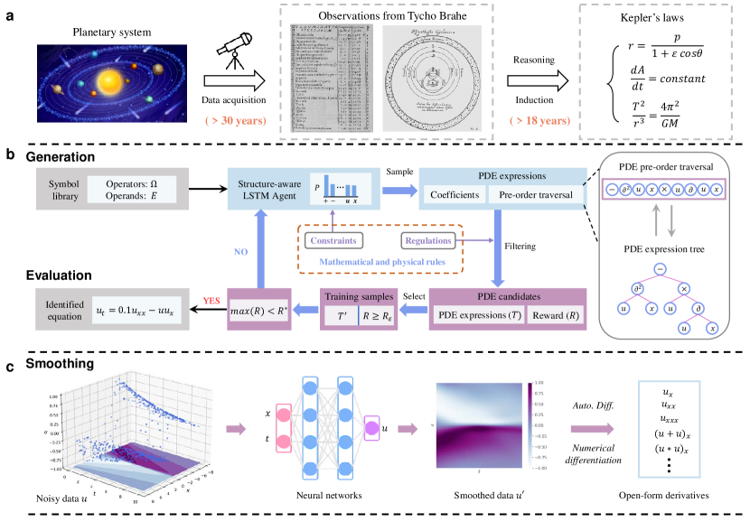
Figure 1: Illustration of the traditional discovery process and DISCOVER. a Discovery of Kepler’s laws. b and c Overview of the DISCOVER framework. b The main working process including generation and evaluation. The symbol library is composed of operators ($\Omega=\{+,-,\times,\div,\land^{2},\land^{3},\partial,\partial^{2},\partial^{3},sin,cos,log\}$ and operands ($E=\{u,x,t,const\}$). The generated PDE traversal sequence can be represented by a unique corresponding PDE tree. $R_{\varepsilon}$ is the $(1-\varepsilon)$-quantile of the rewards of a batch and $R^{*}$ is the predefined reward threshold to terminate the search process. $T$ refers to the generated PDE expression set that conforms to the laws of physics and mathematics, while ${T}^{\prime}$ represents the PDE expressions whose rewards are greater than the threshold $R_{\varepsilon}$, which are also the final training samples utilized to update the agent. c Smoothing procedures (preprocessing part), in which the fully connected neural network is utilized to fit the noisy and sparse observations, so as to smooth data and generate metadata on the rest of the spatial-temporal domain. Numerical differentiation or automatic differentiation is incorporated to evaluate the open-form derivatives.

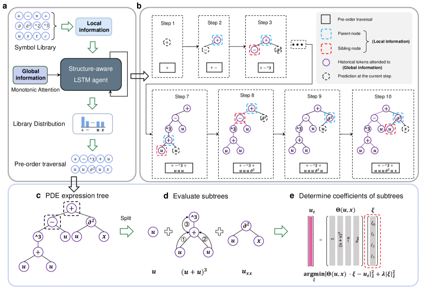
Figure 2: Example of generating a candidate expression $u_{t}=u_{xx}-u+0.1250\left(u+u\right)^{3}$ for the Chafee-Infante equation. a Procedures of generating pre-order traversal of PDE expression trees by the structure-aware LSTM agent based on symbolic representation. The pre-defined symbol library consists of all of the operators and operands to generate the open-form PDEs. Local information and global information are both incorporated during the generation process. The former serves as inputs to the agent explicitly and the latter is utilized by means of monotonic attention in the form of latent variables of aggregated historical information. The output of the LSTM at each time step is the probability distribution of all tokens in the library, and then one of the tokens is sampled based on it. The pre-order traversal sequence is produced aggressively until the terminal condition is satisfied. b The evolution process of local information and global information utilized during the generation process. Local information includes the parent node and sibling node of the current token in the corresponding expression tree. Global information takes historical information in the past into account. c The PDE expression tree is reconstructed from the corresponding pre-order traversal. d Split the expression tree into subtrees according to ($+,-$) operators at the top of the tree, and traverse to calculate each term’s value. e Calculate the coefficients of the function terms based on STRidge.

A nonlinear dynamic system can usually be represented by a parameterized PDE given by:

$$u_{t}=F\left(u,u_{x},u_{xx},\cdots,x,\xi\right)=\Theta(u,x)\cdot\xi$$ (1)

where $u$ is the observations of interest collected from experiments or nature; $u_{t}$ is the first-order time derivative term; and $F$ is a nonlinear function on the right-hand side, consisting of $u$ and its space derivatives with different orders (e.g., $u_{x}$ and $u_{xx}$). The coefficients of those candidate terms in $F$ can be represented by $\xi$. $\Theta(u,x)$ is our target with a more concise form.

The overview of DISCOVER uncovering PDEs from data is demonstrated in Fig. 1b, and comprises two parts: generation and evaluation. The main purpose of the generation process is to first set up a reasonable symbol library and rules to represent PDEs, and then generate PDE expressions through the agent, including the pre-order traversal of PDEs with a tree structure and coefficients of function terms. The former ones are produced autoregressively by sampling the probability distribution of the agent’s output, which is constrained to ensure its rationality in physical and mathematical laws. The latter ones are solved based on the structure of PDE trees and the sparsity-promoting method. During the evaluation stage, the meticulously designed reward function is utilized to evaluate the generated PDE candidates that comply with the customized regulations. Then, the PDE candidates with higher rewards are selected as the training samples. The agent is iteratively updated with the risk-seeking policy gradient method to generate better-fitting expressions until the termination condition is met. Note that observations collected from experiments may be sparse and noisy in real application scenarios. As shown in Fig. 1c, the fully connected neural networks are built to fit and smooth the available data and the metadata are generated to assist the evaluation of derivatives [26] and noise resistance. By introducing this preprocessing part, in essence, the neural network (NN) in DISCOVER is built as a surrogate model to learn the mapping relationship between spatial-temporal inputs and states of interest. It is then analyzed for interpretability and converted into a human-readable format (PDE). In aggregate, DISCOVER can identify open-form governing equations directly from the data, while also possessing high efficiency and scalability. The high efficiency is due to three innovations of our framework: (1) DISCOVER utilizes a structure-aware agent to produce PDE expressions with a tree structure; (2) the coefficients of PDEs are determined by deconstructing the equation tree and combining the sparsity-promoting method to avoid multiple constant optimization processes; and (3) the whole optimization process of generating PDE expressions is neural-guided and parallelizable. In terms of scalability, the symbol library can be easily expanded, and customized constraints and regulations can be incorporated to accelerate the search process according to prior knowledge. Additional details about the frameworks can be found in Methods and Supplementary Information. We will demonstrate the superiority of DISCOVER through canonical problems.

Discovering open-form PDEs of canonical dynamic systems.

We verified the accuracy and efficiency of DISCOVER in mining open-form PDEs containing strong nonlinearities with little prior knowledge. Specifically, we utilized the study cases from previous studies [13, 4, 8, 27], including Burgers’ equation with nonlinear interaction terms, the KdV equation which has high-order derivatives, the Chafee-Infante equation with exponential terms, and the viscous gravity current equation (PDE_compound) with compound function terms and fractional structure (PDE_divide). We use these to test its performance and compare it against a GA-based model (SGA [13]), which is the latest PDE discovery model to handle complex open-form equations. The results show that our framework is not only accurate but also computationally efficient and stable.

Study cases.

Five canonical models of mathematical physics include: (1) The KdV equation: It was jointly discovered by Dutch mathematicians Korteweg and De Vries to describe the one-way wave on shallow water [28]. It takes the form of $u_{t}=auu_{x}+bu_{xxx}$, where $a$ is set to -1, and $b$ is set to -0.0025. (2) Burgers’ equation: As a nonlinear partial differential equation that simulates the propagation and reflection of shock waves, Burgers’ equation is widely used in numerous fields, such as fluid mechanics, nonlinear acoustics, gas dynamics, etc.[29]. We consider a 1D viscous Burgers’ equation $u_{t}=-uu_{x}+vu_{xx}$, where $v$ is equal to 0.1. (3) The Chafee-Infante equation: Another 1D nonlinear system is $u_{t}=u_{xx}+a\left(u-u^{3}\right)$ with $a=-1$, which was developed by Chafee and Infante [30]. It has been broadly employed in fluid mechanics [31], high-energy physical processes [32], electronics [33], and environmental research [34]. (4) PDE_compound and PDE_divide: These two equations are first put forward in SGA and used to demonstrate that our framework is capable of mining open-form PDEs, which is crucial for extracting unidentified and undiscovered governing equations from observations. PDE_compound with equation form $u_{t}=(uu_{x})_{x}$ is proposed to describe viscous gravity currents with a compound function [35]. PDE_divide with equation form $u_{t}=-u_{x}/x+0.25u_{xx}$ contains the fractional structure that conventional closed-library-based methods cannot handle.

The default hyperparameters used to mine the above PDEs are provided in section S1.5 of Supplementary Information. Table 1 shows that under the premise of little prior knowledge, DISCOVER can uncover the analytic representation of the various physical dynamics mentioned above, and the discovered equation form is accurate and concise even with Gaussian noise added. Fig. 3 shows the performance of DISCOVER in the mining equation under the condition of noisy and sparse data. Fig. 3 a-e illustrates the evolution of rewards and function terms of the best expression in the optimization process. For complex equations, there will be redundant or incorrect terms in the generated expressions during iteration (e.g., function term $u$ in Burgers and PDE_divide). However, since model-based optimization is directional, more accurate expressions will be generated as rewards of better cases increase and fewer redundant terms appear. In addition, a risk-seeking policy gradient is utilized and DISCOVER is able to find the optimal result with only the best-case performance considered. Meanwhile, more available data collected contributes to a more accurate surrogate model, and then it is more likely to uncover the correct equation, as shown in Fig. 3f. More discussion on noise and data sparsity can be found in section S2.3 of Supplementary Information. It is worth noting that the KdV equation, Burgers’ equation, and the Chafee-Infante equation can be discovered correctly by conventional sparse regression methods and genetic algorithms, but not for the PDE_compound and PDE_divide equations. This is primarily because these methods rely on a limited set of candidates, and cannot handle equations that contain compound terms or fractional structures. The result demonstrates that our proposed method can directly mine open-form equations from data, which offers wider application scenarios and practicability.

Table 1: Summary of discovered results for different PDEs of mathematical physics. The subscripts $m$ and $n$ denote the number of discretizations. For noisy measurements, 10% noise is added for the KdV, Burgers’, and Chafee-Infante equations, and 1% noise is added for PDE_divide and PDE_compound.

PDE systems	PDE discovered (clean data)	Error (clean, noisy)	Data discretization
KdV	$u_{t}=-0.5001(u\times u)_{x}-0.0025u_{xxx}$	$0.09\pm 0.07\%$, $1.0\pm 1.41\%$	$x\in[-1,1)_{m=512},t\in[0,1]_{n=201}$
Burgers	$u_{t}=-1.0010uu_{x}+0.1024u_{xx}$	$1.34\pm 1.61\%$,$1.59\pm 0.41\%$	$x\in[-8,8)_{m=256},t\in[0,10]_{n=201}$
Chafee-Infante	$u_{t}=1.0002u_{xx}-1.0008u+1.0004u^{3}$	$0.04\pm 0.0\%$,$1.88\pm 0.54\%$	$x\in[0,3]_{m=301},t\in[0,0.5]_{n=200}$
PDE_compound	$u_{t}=0.5002(u^{2})_{xx}$	$0.04\pm 0\%$, $0.05\pm 10\%$	$x\in[1,2)_{m=301},t\in[0,0.5]_{n=251}$
PDE_divide	$u_{t}=-0.9979u_{x}/x+0.2498u_{xx}$	$0.14\pm 0.10\%$, $0.22\pm 0.25\%$	$x\in[1,2)_{m=100},t\in[0,1]_{n=251}$

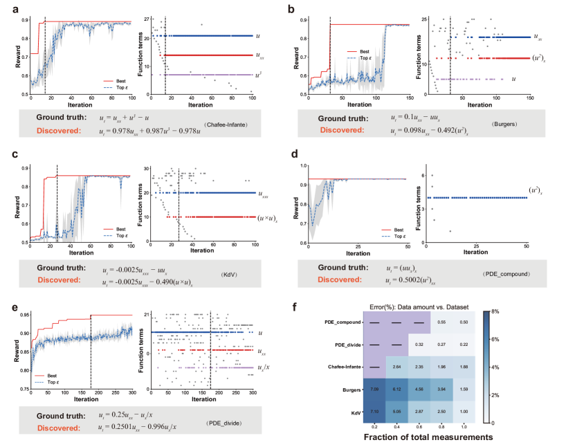
Figure 3: Discovery process of some canonical physical problems with noisy and sparse measurements. a-e: The evolution of rewards and function terms of the best-case expression of a the Chafee-Infante equation, b Burgers’ equation, c the KdV equation, d PDE_compound and e PDE_divide. 10% noise in the first three equations is used, and 1% noise is used in the last two equations. The figure on the left denotes the evolution of the best reward so far and the reward of the top $\varepsilon$ expressions (utilized to update the agent). The figure on the right denotes the evolution of function terms of the best case in the current iteration. Function terms that occur the most are individually marked with colored dots. The gray dashed-line marks the iteration where the expression with maximum reward appears. f Relative error of different physical systems with different volumes of data. Squares marked with a solid black line indicate that the correct form of the equation could not be found.

Comparisons to the GA-based method.

At the expense of flexibility and representation ability, common PDE discovery methods such as SINDy utilize a stationary library and sparse regression to uncover physical laws. Since the stationary library cannot cover or generate all of the complex structures, they are deficient in identifying complex equation forms such as PDEs with fractional structures. For fairness of comparison, the latest symbolic PDE discovery method SGA is taken as an example, which is also capable of uncovering the equation representations of these five physical dynamics correctly. Specifically, we will compare the specific performance (time consumption and accuracy) of DISCOVER based on RL and SGA based on GA. Note that all of the experiments were replicated with five different random seeds for each PDE. As shown in Table 2, the left column represents the MSE between the left-hand and right-hand sides of the discovered equations. A smaller MSE means a more accurate discovered PDE. Both DISCOVER and SGA are capable of mining all terms of the equation exactly, but their coefficients of function terms are slightly dissimilar, resulting in the former having slightly smaller errors than the latter in the first four equations. The right column of Table 2 presents the time consumed by the two methods to identify the optimal equation. It can be seen that, in addition to the Chafee-Infante equation, our method uses only approximately 40% of the time cost by SGA(fast) (a more efficient version) on average, which has higher computational efficiency. This is mainly because our method is model-based, and the entire optimization process is directional with a positive gain. As the iteration proceeds, the generated equations become increasingly reminiscent of the authentic expression. Additional details of the optimization process can be found in section S2.2 of Supplementary Information. In contrast, SGA expands the diversity of the generated equation representations primarily through crossover and mutation of gene fragments, which is more stochastic and uncontrollable. Although it facilitates the search for more complex equations, it also leads to more requisite computational time.

It is worth noting that in the process of uncovering the Chafee-Infante equation, SGA takes $u$ as a default function term (this information itself is known and easily accessible). By introducing this prior knowledge, the optimal form of the equation can always be easily found in the first round of iterations. Without this knowledge, however, SGA is unable to identify the correct form of the equation within 300 iterations (>1000 s). The main reason for this problem is that SGA is modeled based on function terms that are randomly generated, and each function term is represented by a multi-layer tree structure, while the term $u$ is represented as a one-layer root node. In other words, the way that function terms are defined makes SGA prone to produce complex tree structures. However, DISCOVER models the equation as a whole with a pre-order traversal sequence and then partitions it according to the operators ("+" or "-"). The symbol sequence is autoregressively generated and consequently, both simple and complex function terms can be handled easily. It can be seen that our method is time-efficient and has better practicality with little prior knowledge.

Table 2: Comparison of MSE of discovered results and running time for DISCOVER and SGA.

[t] MSE Runing Time (s) DISCOVER SGA DISCOVER SGA SGA(fast)¹ SGA(w/o $u$)² KdV $3.16\times 10^{-5}$ $1.48\times 10^{-4}$ $243.66$ 1464.80 890.50 \ Burgers $4.89\times 10^{-7}$ $4.33\times 10^{-5}$ $206.76$ 495.18 423.8 \ Chafee-Infante $1.36\times 10^{-4}$ $4.72\times 10^{-4}$ 67.23 27.70 $20.12$ >1000 PDE_compound $8.31\times 10^{-6}$ $4.56\times 10^{-5}$ $13.31$ 604.10 557.20 \ PDE_divide $7.64\times 10^{-4}$ $1.78\times 10^{-4}$ $1259.53$ 2046.24 1466.51 \

• SGA(fast) is an optimized version of the original article code, with a faster computation speed.

• SGA(w/o $u$) represents the SGA(fast) version without prior knowledge $u$ provided in advance.

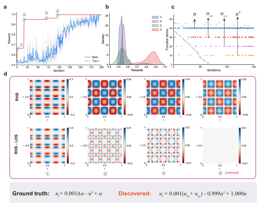
Figure 4: The optimization process and intermediate results at the $40^{th}$ time step of discovering the Allen-Cahn equation. a The distribution of the best-case reward and top $\varepsilon$ fraction of rewards. \scriptsize{1}⃝-\scriptsize{4}⃝  represents the positions where the reward goes through a sharp jump. b The Gaussian kernel density estimate of the top $\varepsilon$ fraction of rewards at \scriptsize{1}⃝-\scriptsize{4}⃝. c Evolution of the function terms of the best expression. The Y-axis corresponds to the 90 most frequent equation terms with decreasing occurrences from the top to the bottom. Each point represents the corresponding function term appearing in the best-case expression produced by the agent at the current iteration step. The four most frequently occurring equation terms are $u$, $u_{xx}$, $u_{yy}$, and $u^{3}$, respectively, which are taken out separately and correspond to function terms of the correct equation form. d The change of the RHS of the mined PDE and the difference between the RHS and LHS ($u_{t}$), which is the residual of the equation.

Discovering complex open-form PDEs of phase separation.

To demonstrate that the proposed DISCOVER framework is capable of mining the high-dimensional PDEs with high-order derivatives, we introduce the Allen-Cahn and Cahn-Hilliard equations, which are firmly nonlinear gradient flow systems and frequently used to describe phase separation processes in fluid dynamics [36, 37, 38] and material sciences[39, 40].

The Allen-Cahn equation.

The 2D reaction-diffusion systems considered here can be represented by $u_{t}=\epsilon^{2}\Delta u-f(u)$, where $\epsilon$ is a small constant value representing the interfacial thickness and $\epsilon^{2}$ is set to 0.001; $\Delta u$ denotes the diffusion term; and $f(u)=u^{3}-u$ represents the reaction term. For this example, Laplace operators appear in the equation in addition to the increase in spatial dimensionality. To ensure that the PDEs mined by DISCOVER conform to the physical laws, we set a constraint on the spatial symmetry of the generated equations that the order of the partial derivatives with respect to the spatial inputs $x$ and $y$ must be the same for the right-hand-side (RHS) term of the equation, i.e., the number of occurrences of $x$ and $y$ in the traversal sequence is the same. Fig. 4a shows the trend of best-case reward and top $\epsilon$ rewards. It can be seen that the best-case reward soon reaches 0.95, and as the iteration proceeds, the reward makes four large jumps in total. According to Fig. 4b the rewards of better-fitting expressions gradually increase at those four jumps. Their discovered equation gradually approaches the ground truth which is demonstrated by Fig. 4d, where the distribution of the RHS of the equations approaches the true distribution, and the gap between the left-hand-side (LHS) term $u_{t}$ and it (i.e., the residual) decreases and finally approaches zero. Fig. 4c illustrates the evolution of the equation terms of the best-case expression during the iterations. As the optimization process proceeds, the gradual increase in the number of equation terms included in the correct equation form proves that the expressions generated by the agent are becoming increasingly accurate while other incorrect function terms gradually disappear.

The Cahn-Hilliard equation.

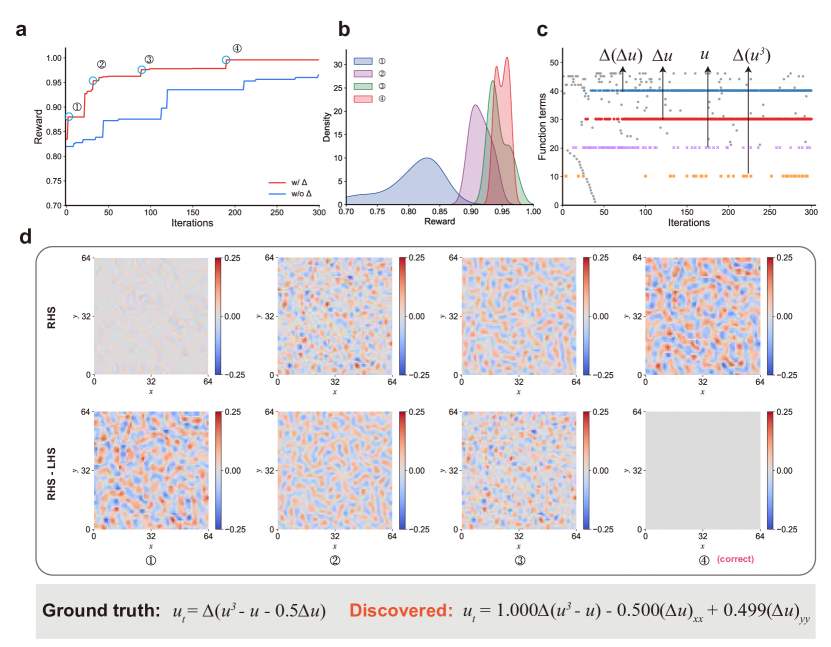
Figure 5: The optimization process and intermediate results at the $250^{th}$ time step of discovering the Cahn-Hilliard equation. a The distribution of the best-case reward and top $\varepsilon$ fraction of rewards. \scriptsize{1}⃝-\scriptsize{4}⃝  represents the positions where the reward goes through a sharp jump. b The Gaussian kernel density estimate of the top $\varepsilon$ fraction of rewards with the Laplace operator at \scriptsize{1}⃝-\scriptsize{4}⃝. c Evolution of the function terms of the best expression. The Y-axis corresponds to the 100 most frequent equation terms with decreasing occurrences from the top to the bottom. The four most frequently occurring equation terms are $\Delta(\Delta u)$, $\Delta u$, $u$, and $\Delta(u^{3})$, respectively. d The change of the RHS of the mined PDE and the difference between the RHS and LHS ($u_{t}$), which is the residual of the equation.

With the fourth order of derivatives and more complicated compound terms, we consider a specific form of Cahn-Hilliard equation $u_{t}=\Delta(u^{3}-u-\kappa\Delta u)$, where $\kappa=0.5$ denotes the surface tension at the interface. The internal term $u^{3}-u-\kappa\Delta u$ within the Laplace operator denotes the chemical potential and has an extremely complicated expansion. For this reason, while retaining the symmetric constraint, we introduce a new Laplace operator in the symbol library and compare it with the default library configuration. It can be seen from Fig. 5a that the reward with the Laplace operator grows faster and can uncover the true equation form in $194^{th}$ iterative steps. However, by the default configuration, the correct equation form can be identified in the $903^{rd}$ iterative steps, which takes more than four times as many iterative steps. Fig. 5b provides the reward distribution of marked iterations and the evolution of function terms is illustrated in Fig. 5c. Note that equation term $u$ mainly appears in the beginning stage of training. With the updating of the agent, the occurrence of redundant term u gradually decreases. The several intermediate results in the evolution process and the values of the RHS term and the residual are also shown in Fig. 5d. The results demonstrate that our framework can seamlessly incorporate possible prior knowledge by expanding constraint and regulation systems or the symbol library to facilitate the searching process and uncover the underlying physical laws in dynamic systems with strong nonlinearity.

These two examples illustrate that DISCOVER can handle high-dimensional and high-order dynamical systems and conveniently introduce new constraints and operators with great scalability to accelerate the discovery process.

Comparisons with other PDE discovery methods.

Table 3: Comparisons of DISCOVER and different methods on the PDE discovery and symbolic regression tasks

Equations	Correct expressions	PDE-FIND  [4]	PDE-NET  [10, 11]	Weak form  [7]	EPDE  [27]	DLGA  [12]	SGA  [13]	DSR  [23, 25]	DISCOVER
KdV	$u_{t}=-uu_{x}-0.0025u_{xxx}$	$\surd$	$\surd$	$\surd$	$\surd$	$\surd$	$\surd$	$\surd$–	$\surd$
Burgers	$u_{t}=-uu_{x}+0.1u_{xx}$	$\surd$	$\surd$	$\surd$	$\surd$	$\surd$	$\surd$	$\surd$–	$\surd$
Chafee-Infante	$u_{t}=u_{xx}+u-u^{3}$	$\surd$	$\surd$		$\surd$	$\surd$	$\surd$	$\surd$–	$\surd$
PDE_compound	$u_{t}=(uu_{x})_{x}$			$\surd$–			$\surd$	$\surd$–	$\surd$
PDE_divide	$u_{t}=-u_{x}/x+0.25u_{xx}$						$\surd$	$\surd$–	$\surd$
Allen-Cahn	$u_{t}=0.001\Delta u-u+u^{3}$	$\surd$	$\surd$	$\surd$	$\surd$	$\surd$	$\surd$–	$\surd$–	$\surd$
Cahn-Hilliard	$u_{t}=\Delta(u^{3}-u-0.5\Delta u)$			$\surd$–			$\surd$–	$\surd$–	$\surd$
Nguyen benchmarks [41]	Nguyen-(1-12)						$\surd$–	$\surd$	$\surd$–

As shown in Table 3, we have presented whether other methods can identify the equations from data mentioned in this article and summarized the boundaries of different methods. Closed library methods including PDE-FIND [4], and PDE-NET [10] and expandable library methods including PDE-NET 2.0 [11], EPDE [27], and DLGA [12] can find the linear combination of possible candidate function terms in the library and are capable of handling the KdV, Burgers, Chafee-Infante, and Allen-Cahn equations. The difference is that the closed library depends more on prior knowledge to ensure that all of the function terms that may appear in the equation are included in the library. Weak-form methods [7] can partly handle the equations with compound terms, but the number of integrals needs to be determined in advance, and fail to deal with multi-layer compound structures. The methods with symbolic representation including SGA [13], DSR [23, 25], and DISCOVER can not only uncover the conventional equations, such as the KdV equation, but also the complex PDEs with compound terms and fractional structures, and symbolic regression tasks. Among them, SGA utilizes GA to expand the search space, but is less efficient and currently confined to 1D dynamics and clean data. DSR and DISCOVER are both based on deep reinforcement learning methods; whereas DSR is designed for symbolic regression tasks whose optimization objective is not consistent with PDE discovery tasks. Specifically, the current DSR neither incorporates the computation of partial differential operators nor is it able to handle sparse and noisy data. The coefficients also cannot be determined efficiently, which may lead to prohibitive computational costs for high-dimensional nonlinear dynamic systems with large data volumes. A detailed description can be found in Supplementary Information S2.4. DISCOVER performs better for PDE discovery tasks as it balances diversity and efficiency in the mining equation process with better scalability. Although not specifically for regression tasks, it can solve most of the symbolic tasks in Nguyen benchmarks [41] under the condition that the appropriate library is defined.

Discussion

We propose a new framework named DISCOVER for exploring open-form PDEs based on enhanced deep reinforcement learning and symbolic representations. It reduces the demand for prior knowledge and is capable of dealing with compound terms and fractional structures that conventional library-based methods cannot handle. The structure-aware architecture proposed is capable of learning the PDE expressions more effectively and can be applied to other problems with structured inputs. Moreover, this framework achieves more efficient and stable performance by means of the neural-guided approach and sparsity-promoting methods compared to GA-based methods (e.g., SGA). In addition to some nonlinear canonical 1D problems (Burgers’ equation with interaction terms, the KdV equation with high-order derivatives, the Chafee-Infante equation with derivative and exponential terms, and PDE_compound and PDE_divide with compound terms and fractional structure, respectively), we also demonstrate this framework on high-dimensional systems with high-order derivatives in the governing equations. Results show that the proposed framework is capable of uncovering the true equation form from noisy and sparse data, and can be applied to solving new tasks efficiently without known physical knowledge incorporated.

Results demonstrated that the proposed framework can assist researchers in different fields to comprehend data and further uncover the underlying physical laws effectively. To extend the boundaries of knowledge and serve a wider range of applications, there are two potential improvements that should be considered in future work. Firstly, despite the optimization efficiency being greatly improved by model-based methods, we still need to reasonably preserve the diversity of the generated equation forms to cope with the potential exploration and exploitation dilemma. Moreover, robustness to noise may be further strengthened with discovered physical knowledge incorporated. Combining the automatic machine learning methods [42, 43] may have the potential to enhance DISCOVER to further identify the open-form PDEs from high-noise and sparse data.

Methods

The steps of DISCOVER mining PDEs mainly consist of three steps: (1) we first build a symbol library and define that a PDE can be represented as a tree structure. A structure-aware recurrent neural network agent by combining structured inputs and monotonic attention is designed to generate the pre-order traversal of PDE expression trees; (2) the expression trees are then reconstructed and split into function terms, and their coefficients can be calculated by the sparse regression method; and (3) all of the generated PDE candidates are first filtered by physical and mathematical constraints, and then evaluated by a meticulously designed reward function considering the fitness to data and the parsimony of the equation. We adopt the risk-seeking policy gradient to iteratively update the agent to improve the better-fitting expressions until the best-case expression meets the accuracy and parsimony requirements that we set in advance. The first two steps correspond to the Generation part, and the third step introduces the Evaluation part in Fig. 1. Additional details are discussed below.

Generating the pre-order traversals of the PDE expression trees.

PDE expression tree.

As shown in Fig. 1a, a PDE can be represented by a binary tree via symbolic representation, and all of the tokens on the nodes are selected from a pre-defined library $\mathcal{L}$. The library consists of two categories of symbols: operators (the first two rows) and operands (the bottom row). Compared with the symbolic regression problem, our library also introduces a differential operator with different orders to calculate the time and space derivatives of state variables. Note that since the LSTM agent is adopted in DISCOVER, which only produces sequential data step by step, pre-order traversal sequences of PDE expression trees are generated in the Generation part.

For a PDE expression tree, the interior nodes are all operators, the leaf nodes are all operands, and their arities are known. For example, the partial derivative $\partial$ is a binary operator with two children, and the space input $x$ is an operand with zero children. This property ensures that each expression tree has a unique pre-order traversal sequence corresponding to it. As a consequence, we can conveniently generate batches of pre-order traversal sequences by means of the LSTM agent instead of the expression trees. An expression tree and its pre-order traversal can be represented as $\tau$. The $i$-th token in the traversal can be represented as $\tau_{i}$ and corresponds to an action under the current policy in reinforcement learning. When generating the token at the current time step, the output of LSTM will be normalized to generate a probability distribution of all tokens in $\mathcal{L}$. The current action is then sampled based on this distribution. A full binary tree is constructed when all leaf nodes in the expression tree are operands, and the generation process is terminated.

Structure-aware LSTM agent.

The common LSTM is an autoregressive model, which means that predicting the current token $\tau_{i}$ is conditioned on the last predicted token $\tau_{i-1}$. Because all of the history information is coupled and stored in a cell, it is insufficient for LSTM to deal with long sequences and structural information. To effectively generate PDE expression trees that have strong structural information, we propose a structure-aware architecture for the LSTM agent. Specifically: (1) the structured input is utilized to convey local information as DSR [23]. For example, as shown in the seventh time step in Fig. 2b, the inputs are its parent ($+$) and sibling (${}^{\wedge}3$), instead of the previous token $u$; and (2) the monotonic attention is leveraged to endow the agent with a more powerful capacity to capture global dependencies and avoids the loss of long-distance information in the step-by-step transmission process. The details of the monotonic attention layer are provided in Supplementary Information S1.2.

Constraints and regulations.

Generating PDE expression sequences in an autoregressive manner without restrictions tends to produce unreasonable samples. To reduce the search space and time consumption, we design a series of constraints and regulations based on mathematical rules and physical laws. Constraints are applied to the agent in its generation of the pre-order traversal sequences and can be divided into two categories, including (1) complexity limits of PDE expressions (e.g., the total length of the sequence shall not exceed the maximum length); (2) relationship limits between operators and operands, e.g., the right child node of partial differential operators (e.g., $\partial$) must be space variables (e.g., $x$) and the left child node of $\partial$ cannot be space variables. In the specific implementation process, these constraints are applied prior to the sampling process, and the probability of the tokens is adjusted directly according to the categories of the violated constraint. In addition to imposing restrictions in the generation period, we also establish a series of regulations to double-check the generated equations and withdraw the unreasonable expressions, e.g., the coefficient of the function term is too small or the overflow of calculation. It is worth noting that regulations are aimed at removing unreasonable function terms, which is conducive to the rationality and simplicity of uncovered equations. This operation is similar to the replacement operations in genetic algorithms (i.e., the function term is set as 0), which to a certain extent increases the diversity of generated equations. Applying these constraints and regulations is convenient and extensible, and can also be incorporated with other domain knowledge for new problems.

Determine coefficients of the PDE expression.

Reconstruct and split the expression tree.

After obtaining the pre-order traversal sequence of the PDE, we first need to reconstruct it into the corresponding tree structure according to the arities of operators and operands. Then, we can split it into subtrees, i.e., the function terms, based on the plus and minus operators at the top of the expression tree, as illustrated in Fig. 2 d and e. Subsequently, we solve for the value of each function term over the entire spatiotemporal domain. In the specific solution process, $\left(u+u\right)^{3}$ in Fig. 2b is taken as an instance. We traverse the subtree from bottom to top in a post-order traversal manner (\scriptsize{1}⃝->\scriptsize{2}⃝->\scriptsize{3}⃝), and then perform operations at each parent node (operators). At this time, the values of its corresponding child nodes have already been calculated.

STRidge.

STRidge is a widely used method in sparse regression, which can effectively determine non-trivial function terms and identify a concise equation by using the linear fit to observations. As shown in Fig. 1e, it can be utilized to solve for the coefficients of each function term based on the results in the previous step. Note that the constant $1$ is incorporated as a default constant term.

$$\xi=\arg\min_{\xi}\left|\Theta(u,x)\cdot\xi-u_{t}\right|_{2}^{2}+\lambda|\xi|_{2}^{2}$$ (2)

where $\lambda$ measures the importance of the regularization term. In order to prevent overfitting, we also set a threshold $tol$, and function terms with coefficients less than $tol$ will be directly ignored. More details can be found in PDE-FIND [4].

It is worth noting that our method aims to solve the coefficients of function terms, and the possible constants in the function terms are not taken into consideration, which is also rare in PDEs. In DSR [23], the constant token is introduced in the library and can be generated by agents. The constant determination is then transformed into the optimization of maximizing reward. Although it has greater flexibility (not necessarily though), the computational burden and time are increased dramatically. Our method is more efficient and more conducive to solving the PDE discovery task. For extreme special situations, we can also incorporate learnable constants in our framework.

Training the agent with the risk-seeking policy gradient method

Reward function.

A complete representation of the generated PDEs, including function terms and their coefficients has been obtained through the above procedures. In order to effectively evaluate the generated PDE candidates, we design a reward function for the PDE discovery problem that comprehensively considers the fitness of observations and the parsimony of the equation. Assuming that the generated PDE expression is $g$, it is formulated as follows:

$$R=\frac{1-\zeta_{1}\times n-\zeta_{2}\times d}{1+RMSE},\quad RMSE=\sqrt{\frac{1}{N}\sum_{i=1}^{N}\left(u_{t_{i}}-g(u_{i},x_{i})\right)^{2}}$$ (3)

where $n$ is the number of function terms of the governing equation; $d$ is the depth of the generated PDE expression tree; $\zeta_{1}$ and $\zeta_{2}$ are penalty factors for parsimony, which are generally set to small numbers without fine-tuning; and $N$ denotes the number of observations. It can be seen that the root mean squared error (RMSE) in the denominator evaluates the fitness of the PDE candidates to the data. The nominator is an evaluation of the parsimony. The former is designed for avoiding overfitting caused by redundant terms and the latter is primarily to prevent unnecessary structures, such as $u/u$.

Risk-seeking policy gradient method.

We adopt the deep reinforcement-learning training strategy to optimize the proposed agent. Herein, the generated PDE expression sequences are equivalent to the episodes in RL, and the generation process of each token corresponds to the selection of actions. Note that the total reward is based on the evaluation of the final sequence, rather than the sum of rewards for each action with a discount factor. The policy $\pi_{\theta}$ refers to the distribution over the PDE expression sequences $p(\tau|\theta)$. Since the generated equations with the highest reward are taken as the final result, we adopt the risk-seeking policy gradient[23] to improve the best-case performance in the training process. The optimization objective of the risk-seeking policy gradient is the expectation of the $\left(1-\varepsilon\right)$- quantile of the rewards $\tilde{q}_{\varepsilon}(R)$, rather than the rewards of all of the samples. Its return is given by:

$$J_{\text{risk}}(\theta;\varepsilon)\doteq\mathbb{E}_{\tau\sim p(\tau\mid\theta)}\left[R(\tau)\mid R(\tau)\geq\tilde{q}_{\varepsilon}(R)\right]$$ (4)

The gradient of the risk-seeking policy gradient can be estimated by:

$$\nabla_{\theta}J_{\text{risk }}(\theta;\varepsilon)\approx\frac{\lambda_{pg}}{\varepsilon N}\sum_{i=1}^{N}\left[R\left(\tau^{(i)}\right)-\tilde{q}_{\varepsilon}(R)\right]\cdot\mathbf{1}_{R\left(\tau^{(i)}\right)\geq\tilde{q}_{\varepsilon}(R)}\nabla_{\theta}\log p\left(\tau^{(i)}\mid\theta\right)$$ (5)

where $N$ denotes the total number of samples in a mini-batch; and $\lambda_{pg}$ measures the importance of rewards. Note that $\tilde{q}_{\varepsilon}$ is also chosen as the baseline reward and varies by the samples at each iteration.

Additional details about the agent, hyper-parameter settings, and the optimization process can be found in Supplementary Information.

Acknowledgement

This work was supported and partially funded by the National Center for Applied Mathematics Shenzhen (NCAMS), the Shenzhen Key Laboratory of Natural Gas Hydrates (Grant No. ZDSYS20200421111201738), the SUSTech – Qingdao New Energy Technology Research Institute, and the National Natural Science Foundation of China (Grant No. 62106116).

Code availability

The implementation details of the whole process are available on GitHub at https://github.com/menggedu
/DISCOVER.

Data availability

All of the data used in the experiments are available on GitHub at https://github.com/menggedu/DISCOVER.

References

- [1] Davies, A. et al. Advancing mathematics by guiding human intuition with ai. Nature 600, 70–74 (2021).
- [2] Kemeth, F. P. et al. Learning emergent partial differential equations in a learned emergent space. Nat. Commun. 13, 3318 (2022).
- [3] Brunton, S. L., Proctor, J. L. & Kutz, J. N. Discovering governing equations from data by sparse identification of nonlinear dynamical systems. Proc. Natl. Acad. Sci. 113, 3932–3937 (2016).
- [4] Rudy, S. H., Brunton, S. L., Proctor, J. L. & Kutz, J. N. Data-driven discovery of partial differential equations. Sci. Adv. 3, e1602614 (2017).
- [5] Shea, D. E., Brunton, S. L. & Kutz, J. N. Sindy-bvp: Sparse identification of nonlinear dynamics for boundary value problems. Phys. Rev. Res. 3, 023255 (2021).
- [6] Kaheman, K., Kutz, J. N. & Brunton, S. L. Sindy-pi: a robust algorithm for parallel implicit sparse identification of nonlinear dynamics. Proceedings of the Royal Society A 476, 20200279 (2020).
- [7] Messenger, D. A. & Bortz, D. M. Weak sindy for partial differential equations. J. Comput. Phys. 443, 110525 (2021).
- [8] Fasel, U., Kutz, J. N., Brunton, B. W. & Brunton, S. L. Ensemble-sindy: Robust sparse model discovery in the low-data, high-noise limit, with active learning and control. Proceedings of the Royal Society A 478, 20210904 (2022).
- [9] Chen, Z., Liu, Y. & Sun, H. Physics-informed learning of governing equations from scarce data. Nat. Commun. 12, 1–13 (2021).
- [10] Long, Z., Lu, Y., Ma, X. & Dong, B. Pde-net: Learning pdes from data. In International Conference on Machine Learning, 3208–3216 (PMLR, 2018).
- [11] Long, Z., Lu, Y. & Dong, B. Pde-net 2.0: Learning pdes from data with a numeric-symbolic hybrid deep network. J. Comput. Phys. 399, 108925 (2019).
- [12] Xu, H., Chang, H. & Zhang, D. Dlga-pde: Discovery of pdes with incomplete candidate library via combination of deep learning and genetic algorithm. J. Comput. Phys. 418, 109584 (2020).
- [13] Chen, Y., Luo, Y., Liu, Q., Xu, H. & Zhang, D. Symbolic genetic algorithm for discovering open-form partial differential equations (sga-pde). Phys. Rev. Res. 4, 023174 (2022).
- [14] Chen, Y. & Zhang, D. Integration of knowledge and data in machine learning. arXiv preprint arXiv:2202.10337 (2022).
- [15] Schmidt, M. & Lipson, H. Distilling free-form natural laws from experimental data. Science 324, 81–85 (2009).
- [16] Augusto, D. A. & Barbosa, H. J. Symbolic regression via genetic programming. In Proceedings. Vol. 1. Sixth Brazilian Symposium on Neural Networks, 173–178 (IEEE, 2000).
- [17] Sun, S., Ouyang, R., Zhang, B. & Zhang, T.-Y. Data-driven discovery of formulas by symbolic regression. MRS Bull. 44, 559–564 (2019).
- [18] Astarabadi, S. S. M. & Ebadzadeh, M. M. Genetic programming performance prediction and its application for symbolic regression problems. Inf. Sci. 502, 418–433 (2019).
- [19] Haeri, M. A., Ebadzadeh, M. M. & Folino, G. Statistical genetic programming for symbolic regression. Appl. Soft Comput. 60, 447–469 (2017).
- [20] Martius, G. & Lampert, C. H. Extrapolation and learning equations. arXiv preprint arXiv:1610.02995 (2016).
- [21] Sahoo, S., Lampert, C. & Martius, G. Learning equations for extrapolation and control. In International Conference on Machine Learning, 4442–4450 (PMLR, 2018).
- [22] Sun, F., Liu, Y., Wang, J.-X. & Sun, H. Symbolic physics learner: Discovering governing equations via monte carlo tree search. In International Conference on Learning Representations (2023).
- [23] Petersen, B. K. et al. Deep symbolic regression: Recovering mathematical expressions from data via risk-seeking policy gradients. In International Conference on Learning Representations (2020).
- [24] Zhang, H. & Zhou, A. Rl-gep: Symbolic regression via gene expression programming and reinforcement learning. In 2021 International Joint Conference on Neural Networks (IJCNN), 1–8 (IEEE, 2021).
- [25] Mundhenk, T. N. et al. Symbolic regression via neural-guided genetic programming population seeding. arXiv preprint arXiv:2111.00053 (2021).
- [26] Xu, H., Chang, H. & Zhang, D. Dl-pde: Deep-learning based data-driven discovery of partial differential equations from discrete and noisy data. Comm. Comput. Phys. 29, 698–728 (2021).
- [27] Maslyaev, M., Hvatov, A. & Kalyuzhnaya, A. V. Partial differential equations discovery with epde framework: application for real and synthetic data. J. Comput. Sci. 53, 101345 (2021).
- [28] Kordeweg, D. & de Vries, G. On the change of form of long waves advancing in a rectangular channel, and a new type of long stationary wave. Philos. Mag 39, 422–443 (1895).
- [29] Burgers, J. M. A mathematical model illustrating the theory of turbulence. Adv. Appl. Mech. 1, 171–199 (1948).
- [30] Newell, A. C. & Whitehead, J. A. Finite bandwidth, finite amplitude convection. J. Fluid Mech. 38, 279–303 (1969).
- [31] Straughan, B. Jordan–cattaneo waves: Analogues of compressible flow. Wave Motion 98, 102637 (2020).
- [32] Mao, Y. Exact solutions to (2+1)-dimensional chaffee–infante equation. Pramana 91, 1–4 (2018).
- [33] Debussche, A., Högele, M. & Imkeller, P. Asymptotic first exit times of the chafee-infante equation with small heavy-tailed lévy noise. Electron. Commun. Probab. 16, 213–225 (2011).
- [34] Korkmaz, A. Complex wave solutions to mathematical biology models i: Newell–whitehead–segel and zeldovich equations. J. Comput. Nonlinear Dyn. 13, 081004 (2018).
- [35] Gardner, G., Downie, J. & Kendall, H. Gravity segregation of miscible fluids in linear models. Soc. Pet. Eng. J. 2, 95–104 (1962).
- [36] Allen, S. M. & Cahn, J. W. A microscopic theory for antiphase boundary motion and its application to antiphase domain coarsening. Acta Metall. 27, 1085–1095 (1979).
- [37] Shen, J. & Yang, X. Numerical approximations of allen-cahn and cahn-hilliard equations. Discrete Contin. Dyn. Syst. 28, 1669 (2010).
- [38] Cahn, J. W. & Hilliard, J. E. Free energy of a nonuniform system. i. interfacial free energy. J. Chem. Phys. 28, 258–267 (1958).
- [39] Bazant, M. Z. Thermodynamic stability of driven open systems and control of phase separation by electro-autocatalysis. Faraday Discuss. 199, 423–463 (2017).
- [40] Khater, M., Park, C., Lu, D. & Attia, R. A. Analytical, semi-analytical, and numerical solutions for the cahn–allen equation. Adv. Differ. Equ. 2020, 1–12 (2020).
- [41] Uy, N. Q., Hoai, N. X., O’Neill, M., McKay, R. I. & Galván-López, E. Semantically-based crossover in genetic programming: application to real-valued symbolic regression. Genet. Program. Evolvable Mach. 12, 91–119 (2011).
- [42] Du, M., Chen, Y. & Zhang, D. Autoke: An automatic knowledge embedding framework for scientific machine learning. IEEE Trans. Artif. Intell. 1–16 (2022).
- [43] Baydin, A. G., Pearlmutter, B. A., Radul, A. A. & Siskind, J. M. Automatic differentiation in machine learning: a survey. J. Mach. Learn. Res. 18, 1–43 (2018).